when do the benefits of using geostatistics for coal...
TRANSCRIPT

When do the Benefits of using
Geostatistics for Coal Resource
Estimation outweigh the Costs ?
Brett Larkin
GeoCheck Pty. Ltd.
Statistical Truisms
Garbage In / Garbage Out
There is no such thing as a free lunch
Statistical analysis of data, rarely if ever,
discovers anything that an experienced data
collector and analyst is not already aware
Statistical analysis of data, can provide the
analyst with numbers to substantiate their case
Potential uses of Geostatistics in
Coal Resource Estimation
There are four areas that analyst consider using Geostatistics in Coal Resource Estimation:
Estimation of coal and overburden volumes and coal quality parameters (kriging)
Confidence limits on the above estimations
Determining where to site additional drill holes
Determining the minimum drill hole spacing for classification of resources as measured, indicated or inferred

Estimation of coal volumes, quality
and overburden
Traditionally, these are estimated using “inverse
distance squared” weightings such as:
0.04 + 0.09 + 0.37 + 0.04 + 0.09 + 0.37 = 1
?
0.37 / 4 = 0.09
0.37 / 1 = 0.37
0.37 / 9 = 0.04
The main disadvantage of inverse distance squared is that it assumes a uniform spatial variability for:
low, medium and high values
all variables
all directions
all seams
all areas
all deposits
The “all directions” can, however, be overcome by performing a transform on the data coordinates but it still leaves the other issues.
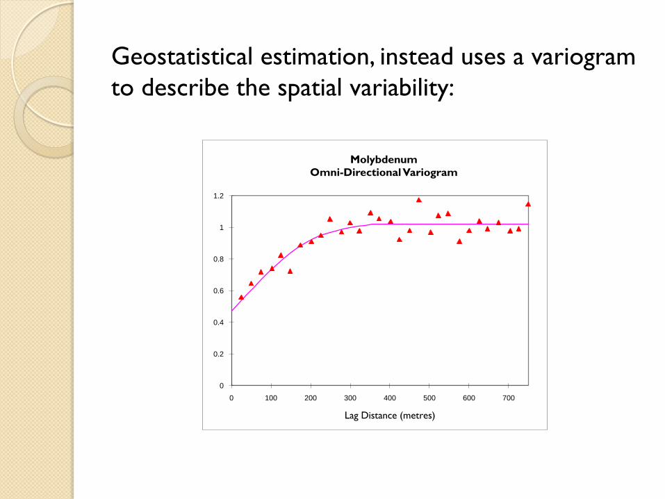
Geostatistical estimation, instead uses a variogram
to describe the spatial variability:
0
0.2
0.4
0.6
0.8
1
1.2
0 100 200 300 400 500 600 700
Molybdenum
Omni-Directional Variogram
Lag Distance (metres)
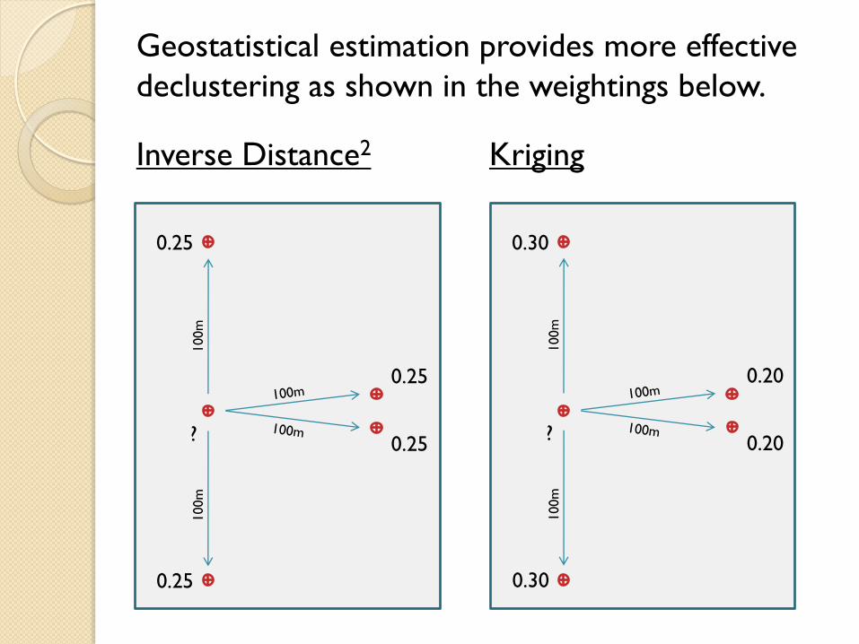
Geostatistical estimation provides more effective
declustering as shown in the weightings below.
Inverse Distance2 Kriging
?
0.25
0.25
0.25
0.25
100m
100m
?
0.30
0.30
0.20
0.20
100m
100m
Benefits
Ability to have different degrees of spatial
inference for different deposits, areas of a
deposit or seams
Ability to have different degrees of spatial
inference for different variables
Ability to have different degrees of spatial
inference for low, medium and high values
Ability to have different degrees of spatial
inference for different directions (??)
More effective declustering of clustered data
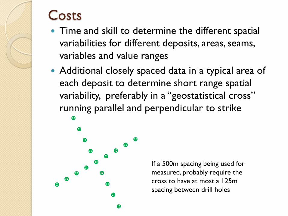
Costs Time and skill to determine the different spatial
variabilities for different deposits, areas, seams,
variables and value ranges
Additional closely spaced data in a typical area of
each deposit to determine short range spatial
variability, preferably in a “geostatistical cross”
running parallel and perpendicular to strike
If a 500m spacing being used for
measured, probably require the
cross to have at most a 125m
spacing between drill holes
WARNING !!!
Geostatistical estimation (kriging) has considerably more “knobs and dials” for controlling the estimate than traditional inverse distance squared approaches.
If the analyst understands what they are doing they can produce a more accurate estimate butif they don’t they can turn the “knobs and dials” the wrong way and produce a considerably less accurate estimate than using the traditional approach.

Estimate of Potential Ranges of
“Actual” Values
Quantitative answers to problems such as:
Confidence limits on estimations
Determining where to site additional drill holes
Determining the minimum drill hole spacing for classification of resources as measured, indicated or inferred
require estimates of what the potential range of “actual” values are at various locations.
This can not be done quantitatively with traditional estimation methods, therefore geostatistics is required for quantitative answer to these questions.
Geostatistics offers two different methods for
determining estimates of the potential range of
“actual” values at various locations.
Estimation variance
Conditional simulation
Estimation variance was the initial method
developed by geostatisticians for determining
these ranges. It is simpler but has a number of
limitations compared to conditional simulation.
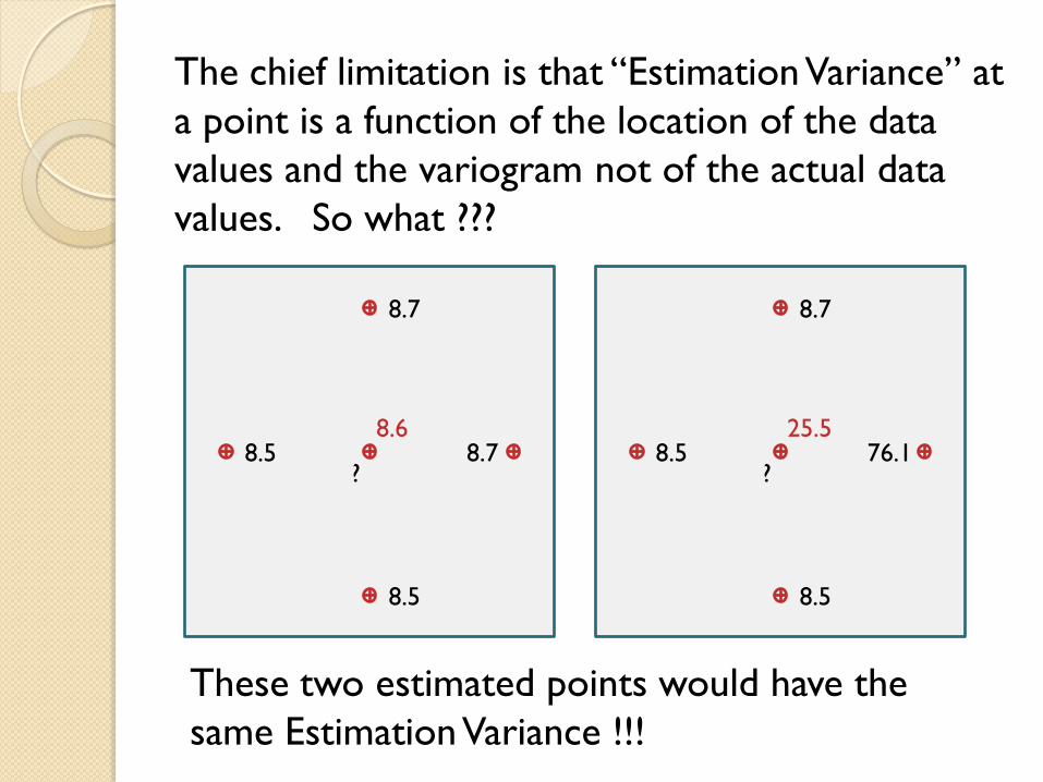
The chief limitation is that “Estimation Variance” at
a point is a function of the location of the data
values and the variogram not of the actual data
values. So what ???
?
8.7
8.5
8.5 8.78.6
?
8.7
8.5
8.5 76.125.5
These two estimated points would have the
same Estimation Variance !!!
The second limitation is that a normal distribution
is generaaly used to turn the estimation variance
into a range of potential “actual values”.
To overcome these issues conditional simulation
was developed by geostatisticians. This not only
uses the variogram and location of data values but
also incorporates the values at data locations.
Why is it called conditional ?
Because it is constrained by the data point values,
that is all realizations honour the data.
What do we mean by realization ?
When analysts estimate block values they accept that this is a smoothing process which gives them an average possible value for each block rather than an actual value.
Further, if you calculate the variogram of estimated block values it will not at all resemble the original variogram.
Conditional simulation uses a random number generator to produce equally likely sets of actual block values. Each of these are called a “realization” and each realization will honour the data values and the variogram.
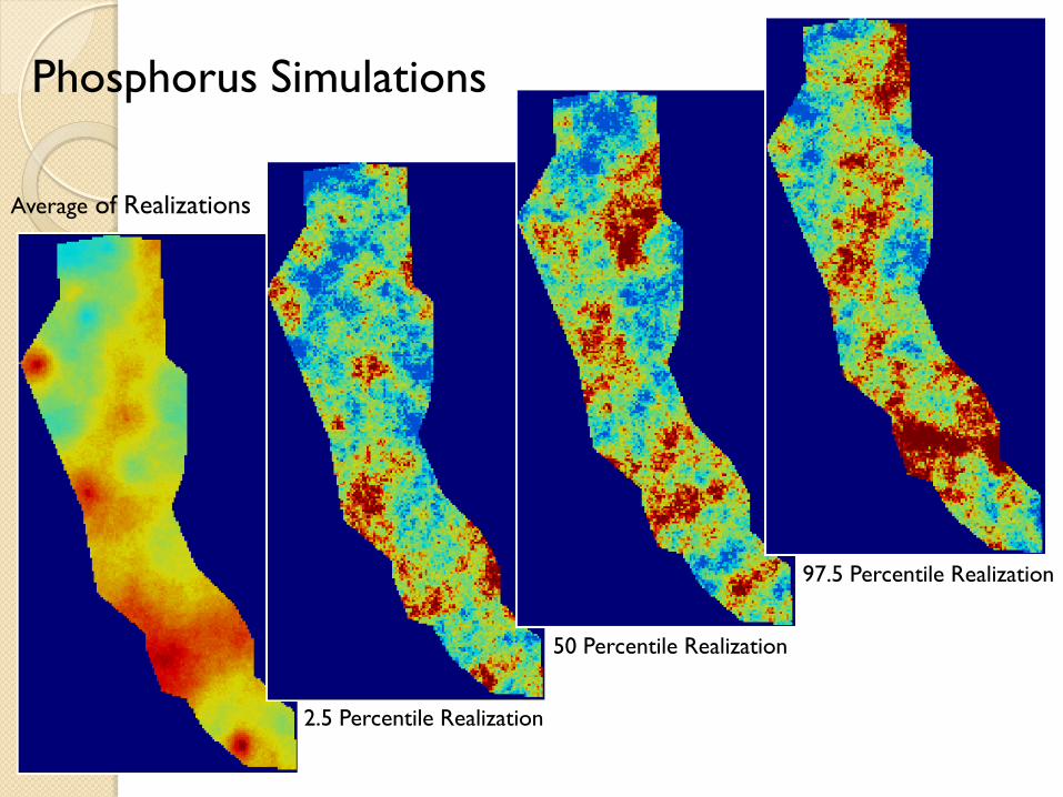
Average of Realizations
2.5 Percentile Realization
Phosphorus Simulations
50 Percentile Realization
97.5 Percentile Realization
With enough realizations the average of the
realizations should be equivalent to the kriged
estimates.
Let us look at the questions we wanted the
simulations to answer.

Confidence Intervals for Estimates
The average of the block values for the 2.5th and
97.5th percentile realization will give us a range for
the deposit’s average sulphur value with a 95
percent confidence.

Benefits
It emphasises that the model is just that and not
reality
Mine planning and contractual arrangements
can be made on worst and best case scenarios
More drilling can be planned if it is felt that the
range of potential values is too large
It provides an explanation when the material is
mined and values are considerably away from
the model estimate
Costs
All the costs mentioned in using geostatistics
for estimation apply
Realizations will only be realistic if the
variograms clearly reflect the deposit, therefore
it may be necessary to augment the drilling to
obtain reliable variograms
It requires even more skill to implement
conditional simulations and ensure they are
realistic than using geostatistics purely for
estimation

Determining where to Site
Additional Drill Holes
For each block in the
simulation, we can
calculate the variance of
the values across all the
realizations and then map
the result.
The high zones on this
map will be where further
drilling is best sited.
Costs and Benefits
This is using a sledgehammer to crack a nut !
Any geologist who knows his trade and the
deposit would come up with a very similar
conclusion with much less effort.
Determining the Minimum Drill Hole
Spacing for Classification of Resources
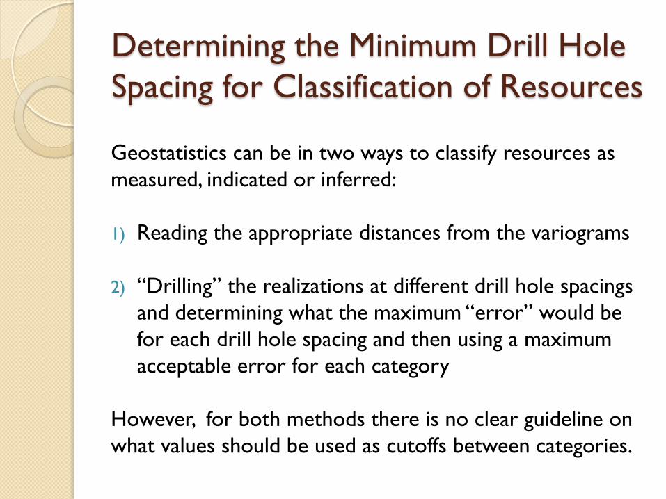
Geostatistics can be in two ways to classify resources as
measured, indicated or inferred:
1) Reading the appropriate distances from the variograms
2) “Drilling” the realizations at different drill hole spacings
and determining what the maximum “error” would be
for each drill hole spacing and then using a maximum
acceptable error for each category
However, for both methods there is no clear guideline on
what values should be used as cutoffs between categories.
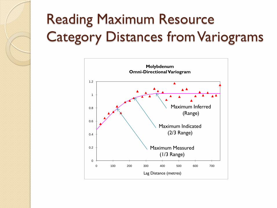
Reading Maximum Resource
Category Distances from Variograms
0
0.2
0.4
0.6
0.8
1
1.2
0 100 200 300 400 500 600 700
Molybdenum
Omni-Directional Variogram
Lag Distance (metres)
Maximum Inferred
(Range)
Maximum Indicated
(2/3 Range)
Maximum Measured
(1/3 Range)

BenefitsThis is a considerable improvement on blindly using
250m, 500m and 1000m for all variables, for all
seams, for all areas across all deposits.
Costs There are no additional costs if you are already
using geostatistics for estimation purposes.
No specific percentages of the range have been
agreed on as the appropriate cutoffs between
categories.
It is not clear how to apply this method where
different variograms are used for low, medium
and high values
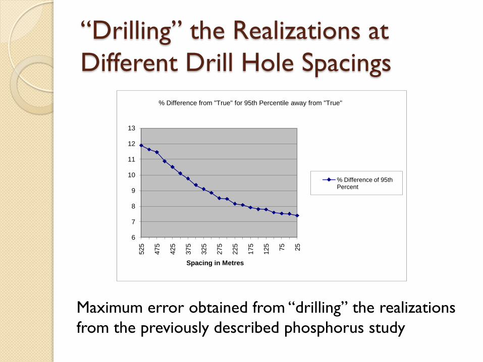
“Drilling” the Realizations at
Different Drill Hole Spacings
Maximum error obtained from “drilling” the realizations
from the previously described phosphorus study
6
7
8
9
10
11
12
13
25
75
125
175
225
275
325
375
425
475
525
Spacing in Metres
% Difference from "True" for 95th Percentile away from "True"
% Difference of 95th Percent
Benefits Possibility of decreasing drilling costs by using a
wider drilling spacing
Determine if necessary to increase drilling spacing
Determine if increasing drilling spacing is going to provide substantial additional information
Costs As well as the costs in performing simulations
additional manipulation of the results is required
No specific percentage differences have been
agreed on as the appropriate cutoffs between
categories.
Conclusion
Geostatistics provides many benefits when calculating resource estimates. Each of these benefits comes at a cost.
For a typical coal resource calculation of just tonnages of coal and cubic metres of overburden the costs of using geostatistics probably outweigh any benefits.
The value of using geostatistics really only comes about where you are dealing with more complex variables such as contaminants and where one requires confidence intervals on one’s results.