When will it break? A Hybrid Soft Computing Model to

Predict Time-to-break Margins in Paper Machines

Piero P. Bonissone and Kai Goebel

General Electric Global Research Center Schenectady, NY 12309, USA

ABSTRACT Hybrid soft computing models, based by neural, fuzzy and evolutionary computation technologies, have been applied to a large number of classification, prediction, and control problems. This paper focuses on one of such applications and presents a systematic process for building a predictive model to estimate time-to-breakage and provide a web break tendency indicator in the wet-end part of paper making machines. Through successive information refinement of information gleaned from sensor readings via data analysis, principal component analysis (PCA), adaptive neural fuzzy inference system (ANFIS), and trending analysis, a break tendency indicator was built. Output of this indicator is the break margin. The break margin is then interpreted using a stoplight metaphor. This interpretation provides a more gradual web break sensitivity indicator, since it uses more classes compared to a binary indicator. By generating an accurate web break tendency indicator with enough lead-time, we help in the overall control of the paper making cycle by minimizing down time and improving productivity. Keywords: Soft Computing, ANFIS, Principal Components, Paper Industry Application.

1. INTRODUCTION

1.1 Soft Computing Soft Computing (SC), sometimes also referred to as Computational Intelligence, was originally defined by Zadeh (1994) as an association of computing methodologies that “…exploit the tolerance for imprecision, uncertainty, and partial truth to achieve tractability, robustness, low solution cost, and better rapport with reality.” According to Zadeh (1998), Soft Computing “includes as its principal members fuzzy logics (FL), neuro-computing (NC), evolutionary computing (EC) and probabilistic computing (PC).” As we remarked in reference (Bonissone 2001b), the main reason for the popularity of soft computing is the synergy derived from its components. In fact, SC’s main characteristic is its intrinsic capability to create hybrid systems that are based on the integration of constituent technologies. This integration provides complementary reasoning and searching methods that allow us to combine domain knowledge and empirical data to develop flexible computing tools and solve complex problems. Soft Computing provides a different paradigm in terms of representation and methodologies, which facilitates these integration attempts. For instance, in classical control theory the problem of developing models is usually decomposed into system identification (or system structure) and parameter estimation. The former determines the order of the differential equations, while the latter determines its coefficients. In these traditional approaches, the main goal is the construction of accurate models, within the assumptions used for the model construction. However, the models’ interpretability is very limited, given the rigidity of the underlying representation language. The equation “model = structure + parameters”, followed by the traditional approaches to model building, does not change with the advent of soft computing. However, with soft computing we have a much richer repertoire to represent the structure, to tune the parameters, and to iterate this process. This repertoire enables us to choose among different tradeoffs between the model’s interpretability and accuracy. For instance, one approach aimed at maintaining the model’s transparency might start with knowledge-derived linguistic models, where the domain knowledge is translated into an initial structure and parameters. Then the model’s accuracy could be improved by using global or local data-driven search methods to tune the structure and/or the parameters. An alternative approach aimed at building more accurate models might start with data-driven search methods. Then, we could embed domain knowledge into the search operators to control or limit the search space, or to maintain the model’s interpretability. Post-processing approaches could also be used to extract more explicit structural information from the models. Extensive coverage of SC components can be found in Back et al. (1997), Fiesler and Beale (1997) and Ruspini et al. (1998). Hybrid SC systems are further described in Bonissone (1997), and Bonissone et al. (1999b).

Proceedings of SPIE 47th Annual Meeting, International Symposium on Optical Science and Technology, Vol. #4787, pp. 53-64, 2002

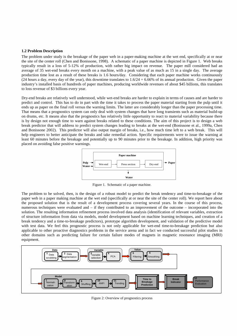
1.2 Problem Description The problem under study is the breakage of the paper web in a paper-making machine at the wet end, specifically at or near the site of the center roll (Chen and Bonissone, 1998). A schematic of a paper machine is depicted in Figure 1. Web breaks typically result in a loss of 5-12% of production, with rather big impact on revenue. The paper mill considered had an average of 35 wet-end breaks every month on a machine, with a peak value of as much as 15 in a single day. The average production time lost as a result of these breaks is 1.6 hours/day. Considering that each paper machine works continuously (24 hours a day, every day of the year), this downtime translates to 1.6/24 = 6.66% of its annual production. Given the paper industry’s installed basis of hundreds of paper machines, producing worldwide revenues of about $45 billions, this translates to loss revenue of $3 billions every year. Dry-end breaks are relatively well understood, while wet-end breaks are harder to explain in terms of causes and are harder to predict and control. This has to do in part with the time it takes to process the paper material starting from the pulp until it ends up as paper on the final roll versus the warning limits. The latter are considerably longer than the paper processing time. That means that a prognostics system can only deal with system changes that have long transients such as material build-up on drums, etc. It means also that the prognostics has relatively little opportunity to react to material variability because there is by design not enough time to warn against breaks related to these conditions. The aim of this project is to design a web break predictor that will address to predict system changes leading to breaks at the wet-end (Bonissone et al., 1999a, Chen and Bonissone 2002). This predictor will also output margin of breaks, i.e., how much time left to a web break. This will help engineers to better anticipate the breaks and take remedial action. Specific requirements were to issue the warning at least 60 minutes before the breakage and potentially up to 90 minutes prior to the breakage. In addition, high priority was placed on avoiding false positive warnings.

Figure 1. Schematic of a paper machine. The problem to be solved, then, is the design of a robust model to predict the break tendency and time-to-breakage of the paper web in a paper making machine at the wet end (specifically at or near the site of the center roll). We report here about the proposed solution that is the result of a development process covering several years. In the course of this process, numerous techniques were evaluated and – if they contributed to an improvement of the outcome – incorporated into the solution. The resulting information refinement process involved data analysis (identification of relevant variables, extraction of structure information from data via models, model development based on machine learning techniques, and creation of a break tendency and a time-to-breakage predictors), prototype algorithm development, and validation of the predictive model with test data. We feel this prognostic process is not only applicable for wet-end time-to-breakage prediction but also applicable to other proactive diagnostics problems in the service arena and in fact we conducted successful pilot studies in other domains such as predicting failure for certain failure modes of magnets in magnetic resonance imaging (MRI) equipment.

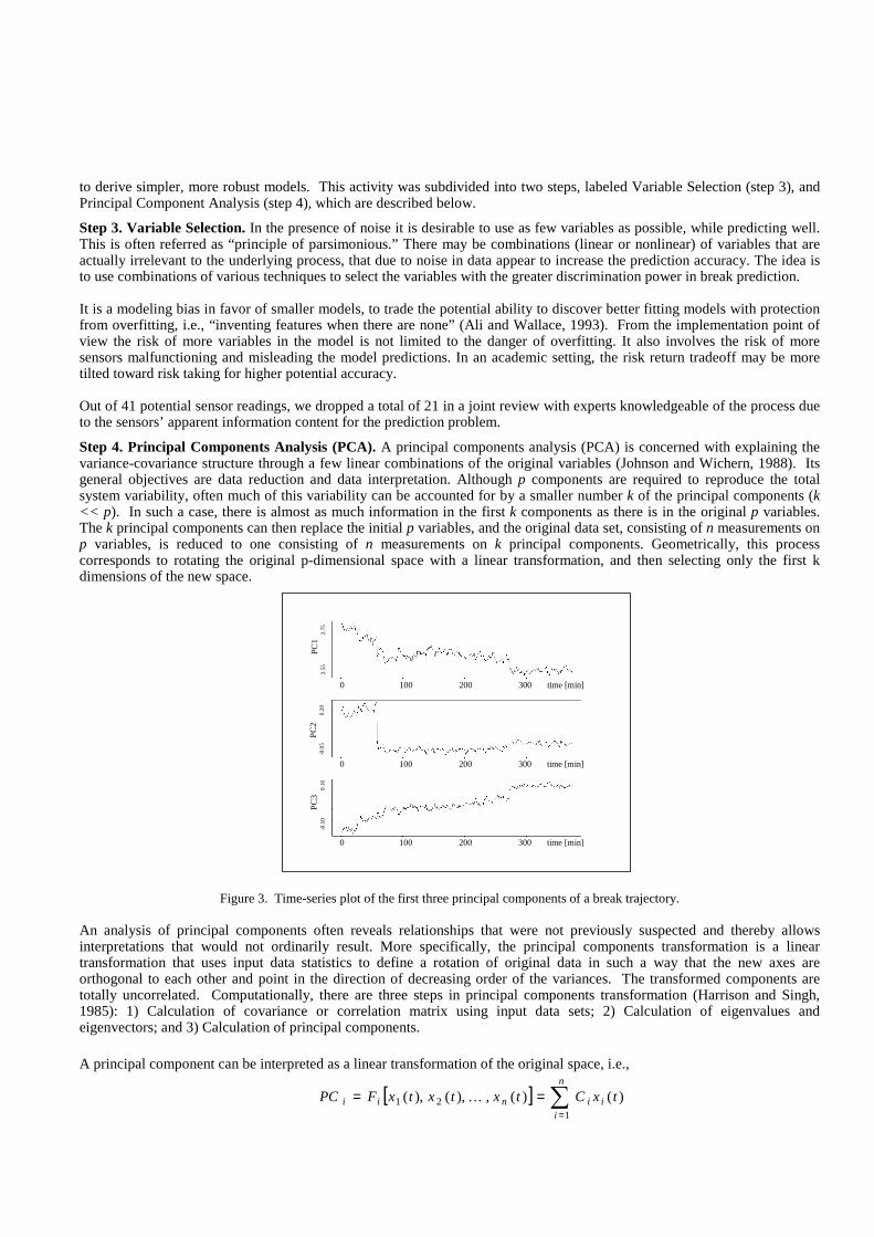
Figure 2: Overview of prognostics process

Datascrubbing

Datasegmentation

1 2Data Reduction

Variable selection

PCA 3 4

Variable Reduction

Filtering Smoothing

5 6Value Transformations

12Performance Evaluation

Break Indicator

Time to Breakage Prediction

Normali-zation

Transform-ation

Shuffling ANFIS

Trending7 8 10 11

Model Generation

9

Pulp

Paper machine

Water

Wet-end Press section Dry-end Paper Water

An overview of the system is schematically represented in Figure 2. There are two modes for the system—training and testing modes. In the training mode, historical web breaks data gathered by sensors are acquired and analyzed, signal processing techniques are applied, and an ANFIS model is fitted to the data off-line. In the testing mode, the sensor readings are analyzed first using the same techniques as in the training phase (except in run-time mode). Next, the ANFIS model takes as input the preprocessed sensor data and gives as output the prediction of time-to-breakage on the fly. This model is used to drive a stoplight display, in which the yellow and red lights represent a 90-minute and 60-minute alarm, respectively.

1.3 Structure of paper In the second section we will describe our proposed multistage process, and we will illustrate the steps in data reduction, variable selection, value transformation, model generation, time-to-break prediction, and break indicator. In the third section we will present the prediction results for the training and validation sets. The last section will contain our concluding remarks and possible future work.

2. SOLUTION DESCRIPTION

2.1 Data Reduction The first activity of our model building process was Data Reduction. Its main purpose was to render the original data suitable for model building purpose. Data were collected during the time period from June 1999 to February 2000. These data needed to be scrubbed and reduced, in order to be used to build predictive models. Observations needed to be organized as time-series or break trajectories. The scope of this project was limited to the prediction of breaks with unknown causes, so we only considered break trajectories associated with unknown causes and eliminated other break trajectories. We needed to separate the trajectories containing a break or recorded in a 180-minute window prior to the break from the ones recorded before such window. Since these two groups formed the basis for the supervised training of our models, we needed to label them accordingly. Most data obtained from sensor readings exhibit some incorrect observations - with missing or zero values recorded for long period of time. These were removed. We did not remove paper grade variability for this particular machine, which was assumed not to cause big variations. This was confirmed upon inspection by an expert team. However, in general, paper grade changes can cause significant changes in process variables and can also be the cause of wet-end breakage. The activity was then subdivided into two steps, labeled “Data Scrubbing” (step 1) and “Data Segmentation” (step 2), which are described below.

Step 1. Data Scrubbing. We grouped the data according to various break trajectories. A break trajectory is defined as a multivariate time-series starting at a normal operating condition and ending at a wet-end break. A long break trajectory could last up to a couple of days, while a short break trajectory could be less than three hours long. We started with roughly 88 break trajectories and 43 variables. Data were grouped according to various break trajectories, namely known break causes and unknown break causes. It was only interesting to consider breaks that could potentially be prevented. This excluded breaks that had known causes such as extremely rare chance events (“observed grease like substance falling on web”), grade changes, machine operation changes, or other non-process failures. After that, we extracted both break negative and positive data from this group. Finally, we deleted incomplete observations and obviously missing values. This resulted in a set of 41 break trajectories.

Step 2. Data Segmentation. After the data scrubbing process, we segmented the data sets into two parts. The first one contained the set of observations taken at the moment of a break and no less than 180 minutes prior to each break. For example, there were a number of breaks occurring in quick succession (break avalanches) which were not suitable for break prediction purposes. Other trajectories contained not the required number of data for other reasons. The resulting remaining data set was denoted as Break Positive Data (BPD). Trajectories that extended beyond 180 minutes were considered to be in steady state (for breakage purposes) and denoted as Break Negative Data (BND). After the data scrubbing and data segmentation, we had break positive data that consisted of 25 break trajectories.

2.2 Variable Reduction The second activity of our model building process was Variable Reduction. Its main purpose was to derive the simplest possible model that could explain the past (training mode) and predict the future (testing mode). Typically, the complexity of a model increases in a nonlinear way with the number of inputs used by the model. High complexity models tend to be excellent in training mode but rather brittle in testing mode. Usually, these models tend to overfit the training data and do not generalize well to new situations - we will refer to this as lack of model robustness. Therefore, a reduction in the number of variables (by a combination of variable selection and variable composition) and its associated reduction of inputs enabled us

to derive simpler, more robust models. This activity was subdivided into two steps, labeled Variable Selection (step 3), and Principal Component Analysis (step 4), which are described below.

Step 3. Variable Selection. In the presence of noise it is desirable to use as few variables as possible, while predicting well. This is often referred as “principle of parsimonious.” There may be combinations (linear or nonlinear) of variables that are actually irrelevant to the underlying process, that due to noise in data appear to increase the prediction accuracy. The idea is to use combinations of various techniques to select the variables with the greater discrimination power in break prediction. It is a modeling bias in favor of smaller models, to trade the potential ability to discover better fitting models with protection from overfitting, i.e., “inventing features when there are none” (Ali and Wallace, 1993). From the implementation point of view the risk of more variables in the model is not limited to the danger of overfitting. It also involves the risk of more sensors malfunctioning and misleading the model predictions. In an academic setting, the risk return tradeoff may be more tilted toward risk taking for higher potential accuracy. Out of 41 potential sensor readings, we dropped a total of 21 in a joint review with experts knowledgeable of the process due to the sensors’ apparent information content for the prediction problem.

Step 4. Principal Components Analysis (PCA). A principal components analysis (PCA) is concerned with explaining the variance-covariance structure through a few linear combinations of the original variables (Johnson and Wichern, 1988). Its general objectives are data reduction and data interpretation. Although p components are required to reproduce the total system variability, often much of this variability can be accounted for by a smaller number k of the principal components (k << p ). In such a case, there is almost as much information in the first k components as there is in the original p variables. The k principal components can then replace the initial p variables, and the original data set, consisting of n measurements on p variables, is reduced to one consisting of n measurements on k principal components. Geometrically, this process corresponds to rotating the original p-dimensional space with a linear transformation, and then selecting only the first k dimensions of the new space.

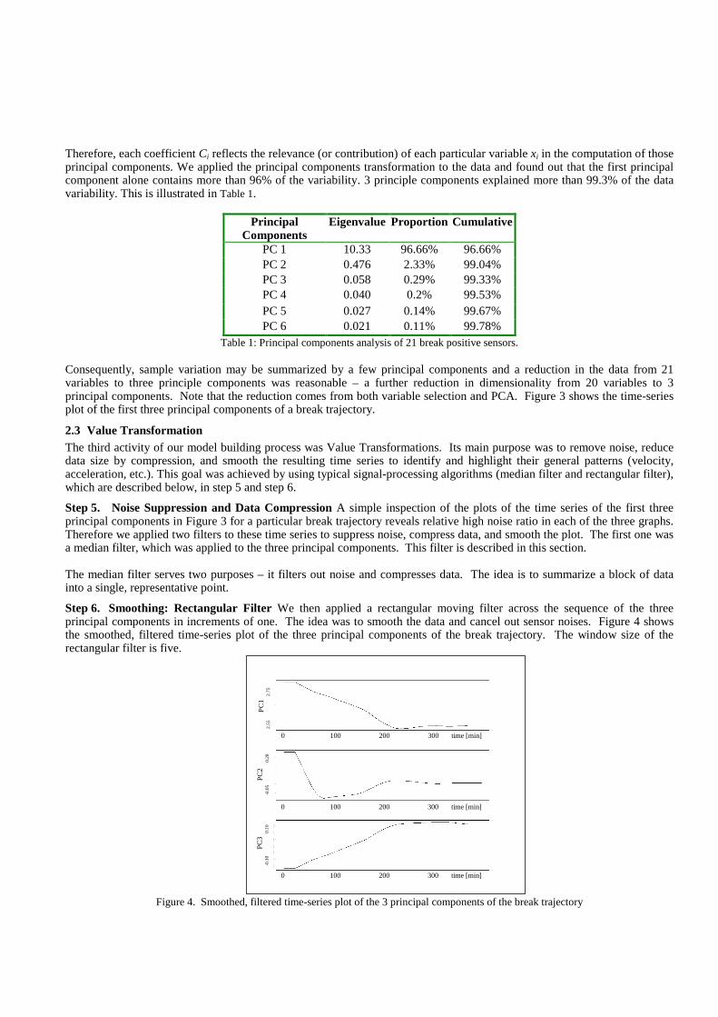
Figure 3. Time-series plot of the first three principal components of a break trajectory.

An analysis of principal components often reveals relationships that were not previously suspected and thereby allows interpretations that would not ordinarily result. More specifically, the principal components transformation is a linear transformation that uses input data statistics to define a rotation of original data in such a way that the new axes are orthogonal to each other and point in the direction of decreasing order of the variances. The transformed components are totally uncorrelated. Computationally, there are three steps in principal components transformation (Harrison and Singh, 1985): 1) Calculation of covariance or correlation matrix using input data sets; 2) Calculation of eigenvalues and eigenvectors; and 3) Calculation of principal components. A principal component can be interpreted as a linear transformation of the original space, i.e.,

0 100 200 300 time [min]

0 100 200 300 time [min]

0 100 200 300 time [min]

PC

12.

552.

75

PC

2-0

.05

0.2

0P

C3

-0.1

00.

10

0 100 200 300 time [min]

0 100 200 300 time [min]

0 100 200 300 time [min]

PC

12.

552.

75

PC

2-0

.05

0.2

0P

C3

-0.1

00.

10

[ ] )()(,),(),(1

21 txCtxtxtxFPC i

n

iinii �

=

== �

Therefore, each coefficient Ci reflects the relevance (or contribution) of each particular variable xi in the computation of those principal components. We applied the principal components transformation to the data and found out that the first principal component alone contains more than 96% of the variability. 3 principle components explained more than 99.3% of the data variability. This is illustrated in Table 1.

Principal Components

Eigenvalue Proportion Cumulative

PC 1 10.33 96.66% 96.66% PC 2 0.476 2.33% 99.04% PC 3 0.058 0.29% 99.33% PC 4 0.040 0.2% 99.53% PC 5 0.027 0.14% 99.67% PC 6 0.021 0.11% 99.78%

Table 1: Principal components analysis of 21 break positive sensors.

Consequently, sample variation may be summarized by a few principal components and a reduction in the data from 21 variables to three principle components was reasonable – a further reduction in dimensionality from 20 variables to 3 principal components. Note that the reduction comes from both variable selection and PCA. Figure 3 shows the time-series plot of the first three principal components of a break trajectory.

2.3 Value Transformation The third activity of our model building process was Value Transformations. Its main purpose was to remove noise, reduce data size by compression, and smooth the resulting time series to identify and highlight their general patterns (velocity, acceleration, etc.). This goal was achieved by using typical signal-processing algorithms (median filter and rectangular filter), which are described below, in step 5 and step 6.

Step 5. Noise Suppression and Data Compression A simple inspection of the plots of the time series of the first three principal components in Figure 3 for a particular break trajectory reveals relative high noise ratio in each of the three graphs. Therefore we applied two filters to these time series to suppress noise, compress data, and smooth the plot. The first one was a median filter, which was applied to the three principal components. This filter is described in this section. The median filter serves two purposes – it filters out noise and compresses data. The idea is to summarize a block of data into a single, representative point.

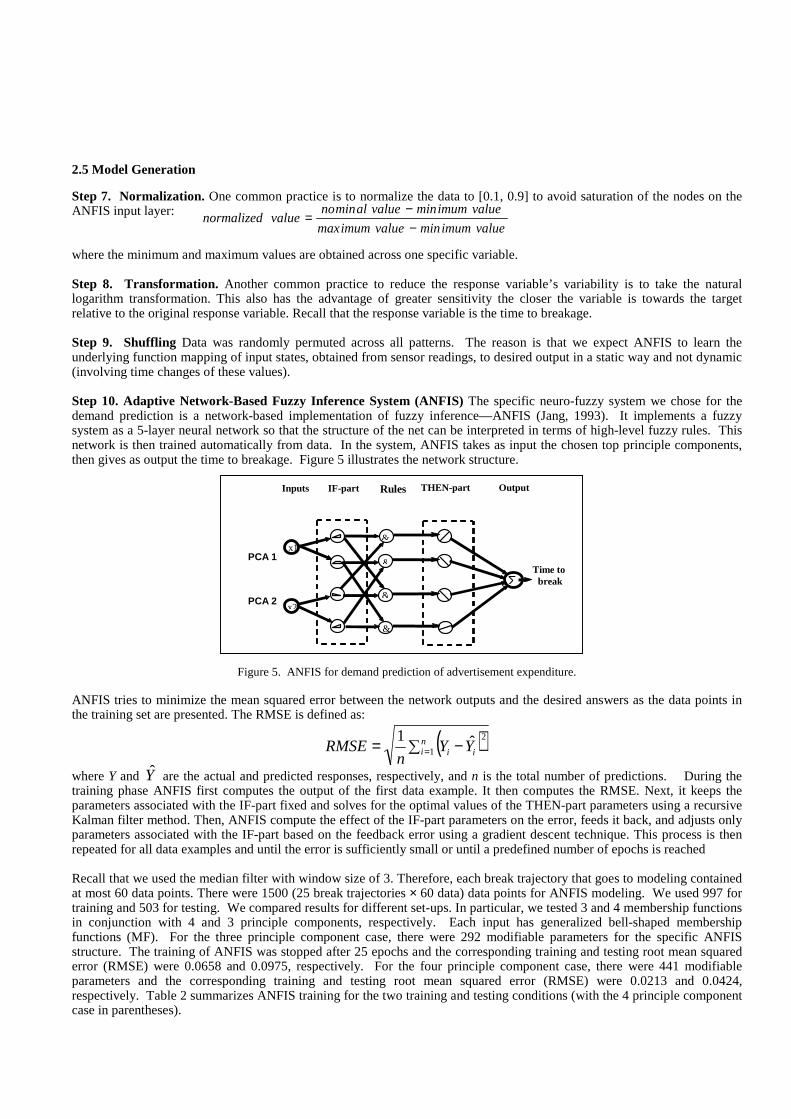
Step 6. Smoothing: Rectangular Filter We then applied a rectangular moving filter across the sequence of the three principal components in increments of one. The idea was to smooth the data and cancel out sensor noises. Figure 4 shows the smoothed, filtered time-series plot of the three principal components of the break trajectory. The window size of the rectangular filter is five.

Figure 4. Smoothed, filtered time-series plot of the 3 principal components of the break trajectory

0 100 200 300 time [min]

0 100 200 300 time [min]

0 100 200 300 time [min]

PC

12

.55

2.7

5

PC

2-0

.05

0.20

PC

3-0

.10

0.1

0

0 100 200 300 time [min]

0 100 200 300 time [min]

0 100 200 300 time [min]

PC

12

.55

2.7

5

PC

2-0

.05

0.20

PC

3-0

.10

0.1

0

2.5 Model Generation

Step 7. Normalization. One common practice is to normalize the data to [0.1, 0.9] to avoid saturation of the nodes on the ANFIS input layer: where the minimum and maximum values are obtained across one specific variable.

Step 8. Transformation. Another common practice to reduce the response variable’s variability is to take the natural logarithm transformation. This also has the advantage of greater sensitivity the closer the variable is towards the target relative to the original response variable. Recall that the response variable is the time to breakage. Step 9. Shuffling Data was randomly permuted across all patterns. The reason is that we expect ANFIS to learn the underlying function mapping of input states, obtained from sensor readings, to desired output in a static way and not dynamic (involving time changes of these values). Step 10. Adaptive Network-Based Fuzzy Inference System (ANFIS) The specific neuro-fuzzy system we chose for the demand prediction is a network-based implementation of fuzzy inference—ANFIS (Jang, 1993). It implements a fuzzy system as a 5-layer neural network so that the structure of the net can be interpreted in terms of high-level fuzzy rules. This network is then trained automatically from data. In the system, ANFIS takes as input the chosen top principle components, then gives as output the time to breakage. Figure 5 illustrates the network structure.

Inputs IF-part Rules THEN-part Output

PCA 1

PCA 2

Time to break

x1

x2

&

&

&

&

Σ

Figure 5. ANFIS for demand prediction of advertisement expenditure.

ANFIS tries to minimize the mean squared error between the network outputs and the desired answers as the data points in the training set are presented. The RMSE is defined as:

( )� −= =ni ii YY

nRMSE 1

2ˆ1

where Y and Y are the actual and predicted responses, respectively, and n is the total number of predictions. During the training phase ANFIS first computes the output of the first data example. It then computes the RMSE. Next, it keeps the parameters associated with the IF-part fixed and solves for the optimal values of the THEN-part parameters using a recursive Kalman filter method. Then, ANFIS compute the effect of the IF-part parameters on the error, feeds it back, and adjusts only parameters associated with the IF-part based on the feedback error using a gradient descent technique. This process is then repeated for all data examples and until the error is sufficiently small or until a predefined number of epochs is reached Recall that we used the median filter with window size of 3. Therefore, each break trajectory that goes to modeling contained at most 60 data points. There were 1500 (25 break trajectories × 60 data) data points for ANFIS modeling. We used 997 for training and 503 for testing. We compared results for different set-ups. In particular, we tested 3 and 4 membership functions in conjunction with 4 and 3 principle components, respectively. Each input has generalized bell-shaped membership functions (MF). For the three principle component case, there were 292 modifiable parameters for the specific ANFIS structure. The training of ANFIS was stopped after 25 epochs and the corresponding training and testing root mean squared error (RMSE) were 0.0658 and 0.0975, respectively. For the four principle component case, there were 441 modifiable parameters and the corresponding training and testing root mean squared error (RMSE) were 0.0213 and 0.0424, respectively. Table 2 summarizes ANFIS training for the two training and testing conditions (with the 4 principle component case in parentheses).

valueimumminvalueimummax

valueimumminvaluealminnovaluenormalized

−−

=

Condition Setting/Result # of trajectories 25 # of total data 1500 # of training data 997 # of testing data 503 # of inputs 3 (4) # of MFs 4 (3) Type of MF Generalized bell-shaped # of modifiable parameters 292 (441) # of epochs 25 Training RMSE 0.0658 (0.0213) Testing RMSE 0.0975 (0.0424)

Table 2: Summary of ANFIS training

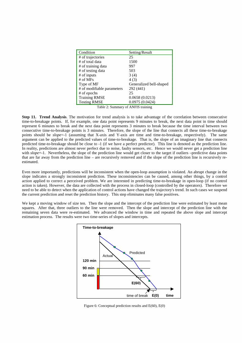
Step 11. Trend Analysis. The motivation for trend analysis is to take advantage of the correlation between consecutive time-to-breakage points. If, for example, one data point represents 9 minutes to break, the next data point in time should represent 6 minutes to break and the next data point represents 3 minutes to break because the time interval between two consecutive time-to-breakage points is 3 minutes. Therefore, the slope of the line that connects all these time-to-breakage points should be slope=-1 (assuming that X-axis and Y-axis are time and time-to-breakage, respectively). The same argument can be applied to the predicted values of time-to-breakage. That is, the slope of an imaginary line that connects predicted time-to-breakage should be close to -1 (if we have a perfect predictor). This line is denoted as the prediction line. In reality, predictions are almost never perfect due to noise, faulty sensors, etc. Hence we would never get a prediction line with slope=-1. Nevertheless, the slope of the prediction line would get closer to the target if outliers –predictive data points that are far away from the prediction line – are recursively removed and if the slope of the prediction line is recursively re-estimated. Even more importantly, predictions will be inconsistent when the open-loop assumption is violated. An abrupt change in the slope indicates a strongly inconsistent prediction. These inconsistencies can be caused, among other things, by a control action applied to correct a perceived problem. We are interested in predicting time-to-breakage in open-loop (if no control action is taken). However, the data are collected with the process in closed-loop (controlled by the operators). Therefore we need to be able to detect when the application of control actions have changed the trajectory's trend. In such cases we suspend the current prediction and reset the prediction history. This step eliminates many false positives.

We kept a moving window of size ten. Then the slope and the intercept of the prediction line were estimated by least mean squares. After that, three outliers to the line were removed. Then the slope and intercept of the prediction line with the remaining seven data were re-estimated. We advanced the window in time and repeated the above slope and intercept estimation process. The results were two time-series of slopes and intercepts.

Figure 6: Conceptual prediction results and E(60), E(0)

Actual Predicted

E(0)

E(60)

60 min

90 min

120 min

time time of break

Time-to-breakage

Then two consecutive slopes were compared to see how far they were away from slope=-1. If they were within a pre-specified tolerance band, e.g. 0.1, we took averages of the two intercepts. In this way, predictions were continuously adjusted according to the slope and intercept estimation. Figure 6 shows the conceptual prediction result.

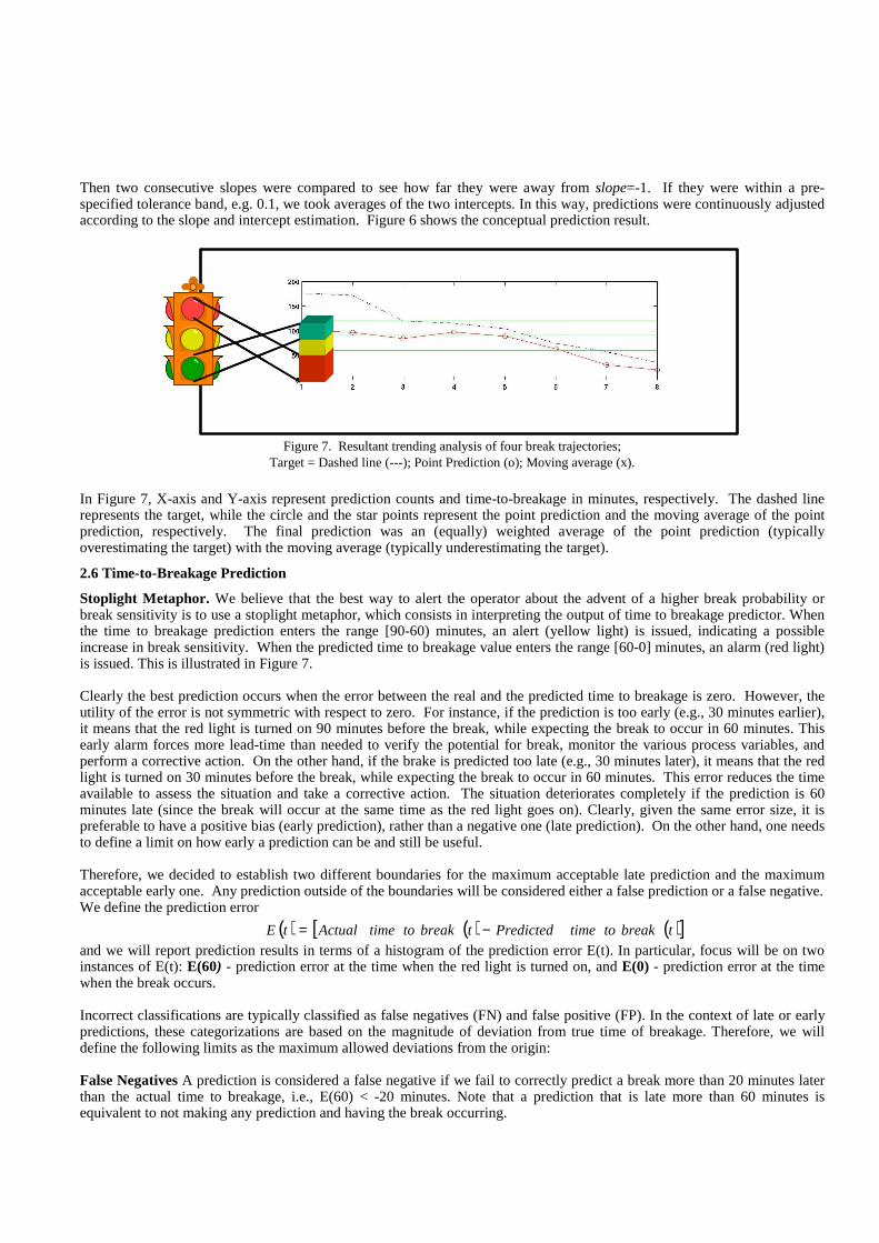
Figure 7. Resultant trending analysis of four break trajectories;

Target = Dashed line (---); Point Prediction (o); Moving average (x).

In Figure 7, X-axis and Y-axis represent prediction counts and time-to-breakage in minutes, respectively. The dashed line represents the target, while the circle and the star points represent the point prediction and the moving average of the point prediction, respectively. The final prediction was an (equally) weighted average of the point prediction (typically overestimating the target) with the moving average (typically underestimating the target).

2.6 Time-to-Breakage Prediction

Stoplight Metaphor. We believe that the best way to alert the operator about the advent of a higher break probability or break sensitivity is to use a stoplight metaphor, which consists in interpreting the output of time to breakage predictor. When the time to breakage prediction enters the range [90-60) minutes, an alert (yellow light) is issued, indicating a possible increase in break sensitivity. When the predicted time to breakage value enters the range [60-0] minutes, an alarm (red light) is issued. This is illustrated in Figure 7. Clearly the best prediction occurs when the error between the real and the predicted time to breakage is zero. However, the utility of the error is not symmetric with respect to zero. For instance, if the prediction is too early (e.g., 30 minutes earlier), it means that the red light is turned on 90 minutes before the break, while expecting the break to occur in 60 minutes. This early alarm forces more lead-time than needed to verify the potential for break, monitor the various process variables, and perform a corrective action. On the other hand, if the brake is predicted too late (e.g., 30 minutes later), it means that the red light is turned on 30 minutes before the break, while expecting the break to occur in 60 minutes. This error reduces the time available to assess the situation and take a corrective action. The situation deteriorates completely if the prediction is 60 minutes late (since the break will occur at the same time as the red light goes on). Clearly, given the same error size, it is preferable to have a positive bias (early prediction), rather than a negative one (late prediction). On the other hand, one needs to define a limit on how early a prediction can be and still be useful. Therefore, we decided to establish two different boundaries for the maximum acceptable late prediction and the maximum acceptable early one. Any prediction outside of the boundaries will be considered either a false prediction or a false negative. We define the prediction error

and we will report prediction results in terms of a histogram of the prediction error E(t). In particular, focus will be on two instances of E(t): E(60) - prediction error at the time when the red light is turned on, and E(0) - prediction error at the time when the break occurs. Incorrect classifications are typically classified as false negatives (FN) and false positive (FP). In the context of late or early predictions, these categorizations are based on the magnitude of deviation from true time of breakage. Therefore, we will define the following limits as the maximum allowed deviations from the origin: False Negatives A prediction is considered a false negative if we fail to correctly predict a break more than 20 minutes later than the actual time to breakage, i.e., E(60) < -20 minutes. Note that a prediction that is late more than 60 minutes is equivalent to not making any prediction and having the break occurring.

( ) ( ) ( )[ ]tbreak to time Predictedtbreak to time ActualtE −=

False Positives A prediction is considered a false positive if we fail to correctly predict a break if the prediction is more than 40 minutes earlier than the actual time to breakage, i.e., E(60) > 40 minutes. We consider this to be excessive lead time, which may lead to unnecessary corrections, for example a slow-down of the machine speed. Although these are subjective boundaries, they seem quite reasonable and reflect the greater usefulness in having earlier rather then later warning/alarms. Step 12. Performance Evaluation The Root Mean Squared Error (RMSE), defined in Section 10, is a typical average measure of the modeling error. However, the RMSE does not have an intuitive interpretation that could be used to judge the relative merits of the model. Therefore, additional performance metrics were used that could aid in the evaluation of the time-to-breakage predictor:

• Distribution of false predictions: E(60) False positives are predictions that were made too early (i.e., more than 40 minutes early). Therefore, time-to-breakage predictions of more than 100 minutes (at time = 60) fall into this category. False negatives are missing predictions or predictions that were made too late (i.e., more than 20 minutes late). Therefore, time-to-breakage predictions of less than 40 minutes (at time =60) fall into this category

• Distribution of prediction accuracy: RMSE Prediction accuracy is defined as the root mean squared error (RMSE) for a break trajectory.

• Distribution of error in the final prediction: E(0) The final prediction by the model is generally associated with high confidence and better accuracy. We associate it with the prediction error at break time, i.e., E(0).

• Distribution of the earliest non false-positive prediction The first prediction by the predictor is generally associated with high sensitivity.

• Distribution of the maximum absolute deviance in prediction This is the equivalent to the worst-case scenario. It shows the histogram of the maximum error by the predictor.

3.0 RESULTS

The model was tested on the data withheld during the shuffling step. It was furthermore validated against independent data sets, both break positive data (BPD) and break negative data (BND). Shown in figure 8 are a.) the histograms for the error before the red zone, b.) final error E(0), c.) earliest valid prediction, and d.) maximum absolute error for the test data set. The most important histograms are the histograms 8.a.) and 8.b.) showing the distribution of E(60) and E(0), i.e., the distribution of the prediction error at the time of the alert (red zone) and at the time of the break. The model tends to slightly underestimate the time-to-breakage. This is a desired feature because it provides a more conservative estimate that does not lead to an incorrect sense of time available for the operator. The mean of the distribution of the final error E(0) is around 20 minutes, (i.e., we tend to predict the break 20 minutes earlier) From the histogram of the earliest final prediction, one can see that reliable predictions can be made, on average, about 150 minutes before the break occurs.

PERFORMANANCE CATEGORY

Train and Test Set for BPD

Validation Set for BPD

Validation Set for BND

Trajectories Total Number of trajectories 25 59 34 Predictions Total Number of Predictions 25 25 34

Correct (Useful) Number of useful

predictions 24 13 34

Number of missed predictions

0 34 0 False Negative

Number of late predictions 1 4 0

False Positive Number of early predictions 0 7 0

Coverage: # Predictions/ # Trajectories 100.00% 42.40% 100%

Relative Accuracy: # Correct predictions/#

Predictions 96.00% 52.00% 100%

Global Accuracy:

# Correct predictions/# Trajectories 96.00% 22.05% 100%

Table 3: Analysis of the Histograms E(60) - Error Before Red Zone and E(0) - Final Error

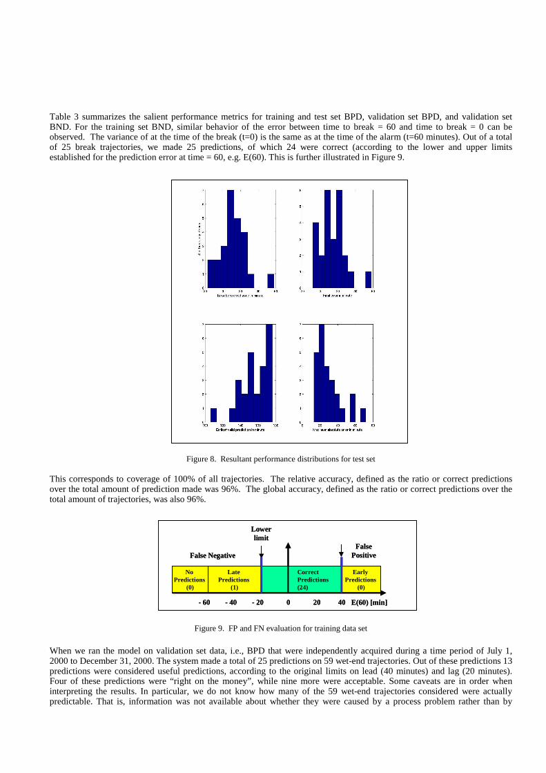
Table 3 summarizes the salient performance metrics for training and test set BPD, validation set BPD, and validation set BND. For the training set BND, similar behavior of the error between time to break = 60 and time to break = 0 can be observed. The variance of at the time of the break (t=0) is the same as at the time of the alarm (t=60 minutes). Out of a total of 25 break trajectories, we made 25 predictions, of which 24 were correct (according to the lower and upper limits established for the prediction error at time = 60, e.g. E(60). This is further illustrated in Figure 9.

Figure 8. Resultant performance distributions for test set This corresponds to coverage of 100% of all trajectories. The relative accuracy, defined as the ratio or correct predictions over the total amount of prediction made was 96%. The global accuracy, defined as the ratio or correct predictions over the total amount of trajectories, was also 96%.

Figure 9. FP and FN evaluation for training data set

When we ran the model on validation set data, i.e., BPD that were independently acquired during a time period of July 1, 2000 to December 31, 2000. The system made a total of 25 predictions on 59 wet-end trajectories. Out of these predictions 13 predictions were considered useful predictions, according to the original limits on lead (40 minutes) and lag (20 minutes). Four of these predictions were “right on the money”, while nine more were acceptable. Some caveats are in order when interpreting the results. In particular, we do not know how many of the 59 wet-end trajectories considered were actually predictable. That is, information was not available about whether they were caused by a process problem rather than by

Early Predictions

(0)

No Predictions

(0)

E(60) [min]0 20 40- 20- 40- 60

Late Predictions

(1)

Correct Predictions (24)

FalsePositiveFalse Negative

Lower limit

Early Predictions

(0)

No Predictions

(0)

E(60) [min]0 20 40- 20- 40- 60

Late Predictions

(1)

Correct Predictions (24)

FalsePositiveFalse Negative

Lower limit

equipment failure, scheduled breaks, foreign objects falling on web, etc.). Visual inspection of first versus second principal components for the trajectories shows very different patterns among them – which might indicate different break modes and causes. In addition, there is a six months gap between the training set used to build the model and the validation test. Such a long period tends to degrade the model performance. In on-line mode, we would have used part of the new break trajectories to update the model. The process has been further validated when we applied it to a second data set with break negative data (BND) to validate against false positive generation during steady state operation. Out of 34 data sets, no false positives were generated. There were a number of slopes trending downward (17) for short periods of time (less than 10 minutes each) which are attributable to “normal” process variations and noise not indicative of impending wet end breaks. In addition, they might be attributed to the close-loop nature of the data: the human operators are closing the loop and trying to prevent possible breaks, while the model is making the prediction in open-loop, assuming no human intervention.

4.0 SUMMARY AND CONCLUSIONS We have developed a systematic process for building a predictive model to estimate time-to-breakage and provide a web break tendency indicator in the wet-end part of paper machines used in paper mills. The process is based on sensor readings coupled with data analysis, principal component analysis (PCA), adaptive network based fuzzy inference system (ANFIS), and trending analysis. The process is summarized by the following twelve components—data scrubbing, data segmentation, variable selection, principal components analysis, filtering, smoothing, normalization, transformation, shuffling, ANFIS modeling, trending analysis and performance evaluation. This process generates a very accurate model that minimizes false alarms (FP) while still providing an adequate coverage of the different type of breaks caused by unknown causes. The system and process to indicate wet-end break tendency and to predict time-to-breakage takes as input sensor readings and produces as output the "time-to-breakage" or break margin, i.e., how much time is left prior to a wet-end break. This break margin is then interpreted using a stoplight metaphor. When the papermaking process leaves its normal operation region (green light) the system issues warnings (yellow light) and alarms (red light). This interpretation provides a more intuitive web break sensitivity indicator, since it uses more than just two classes. These are very significant results, since, in the original scope of this project we were not concerned with False Negatives, i.e., we were not concerned with providing a complete coverage of all possible breaks with unknown causes. In fact, in the early phase of the project we decided to focus on a subset of breaks (caused by stickiness). We then discussed the possibility of covering up to 50% of breaks with unknown causes. In the later stages of the project, when providing time-to-breakage estimates, we relaxed this constraint. However, it is still the case that we are not expecting a complete coverage of all possible wet-end breaks. Predictive models must be maintained over time to guarantee that they are tracking the dynamic behavior of the underlying (papermaking) process. Therefore, we suggest to repeat the steps of the model generation process every time that the statistics for coverage and/or accuracy deviate considerably from the ones experienced in this report. It is also suggested to reapply the model generation process every time that a significant number of new break trajectories (say, twenty) with unknown causes, associated with the wet-end part of the machine. To improve the results further, we feel that increasing the information content of the 2nd and 3rd principle component would be helpful. This means that less correlated data need to be acquired which can be accomplished through other process variables including chemical data and external variables, such as “time since felt change”, etc. In addition, this particular study used a rather small amount of break trajectories for training which to develop a model that can provide better generalization. Current feedback of break cause for the trajectories is sparse and not always correct. We do not want to pollute the model by trying to learn scheduled downtimes, mechanical failures, etc. Therefore, a best practice would be proper annotation that would allow the elimination of improper trajectories from the training set to properly segment trajectories for model development and to construct a more informative validation set. Finally, we would consider the use of additional feature extractions and classification techniques and their fusion to improve the classification performance (Goebel, 2001).

5.0 REFERENCES Ali, Ö. Gür and Wallace, W. A. (1993). Induction of Rules Subject to Quality Constraints: Probabilistic Inductive Learning, IEEE Transactions on Knowledge and Data Engineering, vol. 5, pp. 979-984. Back T, Fogel DB and Michalewicz Z (1997). Handbook of Evolutionary Computation, Bristol, UK: Institute of Physics, and New York, NY: Oxford University Press. Bonissone P. (1997). Soft Computing: the Convergence of Emerging Reasoning Technologies, Soft Computing - A Fusion of Foundations, Methodologies and Applications, Springer-Verlag, Vol. 1, no. 1, pp. 6-18. Bonissone P, Chen YT, and Khedkar P. (1999a). System and method for predicting a web break in a paper machine. US Patent 5,942,689, August, 1999. Bonissone P, Chen Y-T, Goebel K and Khedkar P (1999b). Hybrid Soft Computing Systems: Industrial and Commercial Applications, Proceedings of the IEEE, pp 1641-1667, vol. 87, no. 9, September 1999. Bonissone P and Goebel K (2001a). Soft Computing for Diagnostics in Equipment Service, Proceedings of IFSA/NAFIPS, Vancouver, BC, July. 2001. Bonissone P (2001b). Soft Computing Applications at General Electric, Proceedings of SPIE (4479) Applications and Science of Neural Networks, Fuzzy Systems and Evolutionary Computation IV, pp. 165-176, San Diego, CA, Aug. 2001 Chen Y.T. and Bonissone P (1998). Industrial applications of neural networks at General Electric, Technical Information Series, 98CRD79, GE Corporate R&D, October, 1998. Chen Y.T. and Bonissone P (2002). System and method for paper web time-break prediction. US Patent 6,405,140, June, 2002. Fiesler E. and Beale R (1997). Handbook of Neural Computation, Institute of Physics, Bristol, UK and Oxford University Press, NY. Goebel K. (2001). Architecture and Design of a Diagnostic Information Fusion Tool, AIEDAM: Special Issue on AI in Equipment Service, pp. 335-348, 2001. Jang, J.S.R.(1993). ANFIS: Adaptive-Network-Based Fuzzy Inference System, IEEE Trans. Systems, Man, Cybernetics, 23(5/6), pp. 665-685, 1993. Johnson, R.A. and Wichern, D.W (1988). Applied Multivariate Statistical Analysis, Prentice Hall, 1988. Ruspini E, Bonissone Pand Pedycz W. (1998). Handbook of Fuzzy Computation, Institute of Physics, Bristol, UK. Singh A, and Harrison A (1985). Standardized principal components, International Journal of Remote Sensing, No. 6, pp.989-1003. .