why do firms fail? managerial acquisitiveness and ...economics.ca/2008/papers/0489.pdfwhy do firms...
TRANSCRIPT

Why Do Firms Fail?
Managerial Acquisitiveness and Corporate Failure
Mohammad M. Rahaman∗
April 30, 2008
Abstract
Can managerial actions precipitate corporate failure? In this paper, we focus on an important but easily identifiablemanagerial action, i.e. mergers and acquisitions (M&A), whose effect on firm value is arguably random as shownby the empirical corporate finance literature. We show that for a sample of industrial firms that use the M&Ainvestment technology to pursue aggressive corporate growth strategies, excessive acquisitiveness relative to themedian industry counterpart can aggravate firms’ failure hazard. After removing the failure risk arising fromvarious industry and aggregate economic disturbances, a one standard deviation increase around the mean of theexcessive acquisitiveness measure augments the conditional failure risk by 61% (conditional on other exogenousvariables evaluated at the mean). We find that excessively acquisitive firms shrink in market value, sink inoperating performance, and dislodge the balance between firms’ debt and assets structure by taking on more shortterm debt with less liquid assets at hand between the periods of their intense M&A activities. This mismatchbetween debt maturity and asset liquidity also explains why excessive acquisitiveness can pave the way to corporatedefault: a one standard deviation increase around the mean of the excessive acquisitiveness measure increases theconditional default risk by 34% (conditional on other exogenous variables evaluated at the mean) after controllingfor various determinants of financial distress that are widely used in the bankruptcy prediction literature. Usinga mediating instrument methodology, we argue that the causality from the excessive use of M&A to the firm-failure is channeled through amplified business risk along with managerial cognitive bias and limited attentionspan. The mediation process seems to be stronger through the behavioral channel than the risk channel. Finally,we document capital market myopia in disciplining excessively acquisitive managers - although the market, onaverage, punishes aggressive acquirers at the time of the bid announcement, it does not do so at all quantiles of theconditional distribution of acquirers’ cumulative abnormal return from announcement events. However, despitethis seeming myopia, the external corporate control market eventually reins in the excessive acquirers by turningthem into future targets of takeover.
JEL Classification: G33, G34Key Words: Corporate Failure, Mergers and Acquisitions, Corporate Default
∗Department of Economics and Rotman School of Management, University of Toronto, Email: [email protected]

M.M. Rahaman Corporate Failure
1 Introduction
Can managerial actions precipitate corporate failure? As the business climate deteriorates or the guidanceof the firm falls into the hands of people with less energy and less creative genius, the firm starts sinkingdeep into troubled water and there comes a time when continuing the money losing operation becomestoo painful to bear and failure becomes imminent. Managers may buy some time to save the sinking shipby liquidating assets to finance their excessive continuation, but as the liquidity runs out the inevitablereckoning with failure strikes hard and equity holders are faced with the ultimate decision of being acquiredor going bankrupt. Unfortunately, this scenario is all too common in the modern corporate landscape. Yet,our understanding of the causes of failure is very limited even though this issue bears tremendous importancefor investors, managers, and policy-makers alike.
In this paper, we focus on an important but easily identifiable managerial action, i.e. mergers and acquisi-tions (M&A) bids, whose effect on firm value is arguably random as shown by the empirical corporate financeliterature. However, the M&A actions do entail real and financial consequences on firms. We investigate (i)whether the excessive use of M&A investment technology relative to an industry benchmark can precipitatecorporate failure, and if it does, (ii) what the possible channels are through which it catalyzes the eventualfailure of firms.1 Mergers and acquisitions are widely-used investment technologies at the disposal of man-agers pursuing aggressive corporate growth strategies. In recent years, M&A deals have been ballooning bothin terms of value and volume2, although empirical evidence in corporate finance shows that three-quarters ofmergers and acquisitions never pay off - the acquiring firm’s shareholders lose more than the acquired firm’sshareholders gain [Lovallo and Kahneman (2003)]. In a recent article, Moeller, Schlingemann and Stulz(2005) document that during the recent merger wave in the U.S. shareholders’ values have been destroyedon a massive scale squandering more value in absolute dollar term than the value destruction due to M&Aduring all of the 1980s.3 It is thus puzzling to see these flurries of M&A deals when we know that potentialvalue creation for the shareholders from this investment technology is at best random. When a number offirms create value through M&A while an equal or greater number of firms destroy value using the sameinvestment technology, on average, we may not see any identifiable effect of M&A investment technologyon firm value. On the other hand, comparing a treatment sample of acquirers with a control sample ofnon-acquirers confounds the identification through selectivity and due to the arguably random effect of thetreatment (in this case M&A) on firm value. To meaningfully relate the hazard of corporate failure withthe managerial M&A actions, our identification strategy focuses on a particular sample of firms that use theM&A investment technology to pursue their corporate growth strategies and investigate whether firms thatuse this technology more aggressively than the typical firm in the industry fail more often than firms that
1We use ‘excessive use of M&A’ and ‘aggressive use of M&A’ interchangeably in this paper. We define the precise measureof ‘excessive acquisitiveness’ in the data section of the paper. Succinctly, ‘excessive acquisitiveness’ is defined to be the degreeof managerial acquisitiveness that is greater than the median firm in the industry.
2According to recent statistics by Thomson Financial, deals involving U.S. targets totaled $845 billion during the first fivemonths of 2007, 53% of the total for 2006, and 10% more than deal value in the entire first half of 2006. At the same time,the value of M&A deals in Canada almost doubled from $89 billion to $173.6 billion (expressed in US dollars) by January 2007and the number of deals increased by 26%.
3Moeller, Schlingemann and Stulz (2005) show that acquiring-firm shareholders lost 12 cents around acquisition announce-ments per dollar spent on acquisitions for a total loss of 240billionfrom1998through2001, whereastheylost7 billion in all of the1980s, or 1.6 cents per dollar spent. The 1998 to 2001 aggregate dollar loss of acquiring-firm shareholders is so large because ofa small number of acquisitions with negative synergy gains by firms with extremely high valuations. Without these acquisitions,the wealth of acquiring-firm shareholders would have increased. Firms that make these acquisitions with large dollar lossesperform poorly afterwards.
2

M.M. Rahaman Corporate Failure
utilize this technology conservatively relative to the same industry benchmark.4 This research contributesto the existing literature in two ways. First, it addresses the yet unresolved question in corporate financeof whether using the M&A investment technology necessarily creates value for the corporate stakeholders inthe long run and the mechanism through which the excessive use of M&A investment technology creates ordestroys firm value. Second, by linking managerial excessive use of M&A investment technology with firmfailure, it tries to shed light on the age old debate in finance of whether managers of the failed businessesare villains or scapegoats.
Although conventional wisdom in corporate finance suggests that M&A necessitate an alteration in a firm’sinvestment and financial policies, debates on what shake and shape the firm level resource reallocationthrough this mechanism remain vibrant to this day. Managers may acquire new capital through M&Ainstead of building up internally if the external economic disturbances alter the underlying economic funda-mentals within the industry and render the existing asset structure suboptimal. In that sense, managerialacquisitiveness is a rational response to changes in broad economic fundamentals.5 On the other hand, bullmarkets may lead groups of bidders with overvalued stock to use the stock to buy real assets of undervaluedtargets through mergers and acquisitions. In that sense, managerial acquisitiveness is essentially the man-agerial acumen to time the market to create windfall value for the shareholders.6 Irrespective of what drivesmanagerial acquisitiveness, in a world without frictions and agency problems, access to M&A investmenttechnology helps managers to achieve the optimal asset structure faster in response to deregulation andchanges in economic fundamentals in turn creating value for the shareholders. However, in the presenceof frictions and agency problems within the firm, it is not obvious whether having access to M&A invest-ment technology will always create value for the shareholders, let alone the aggressive use of this investmenttechnology. In fact, one can argue from the empirical literature in corporate finance that value creationthrough M&A in the short run and long run is at best random - some firms create value while an equalor greater number of firms also destroy value. Although value creation and destruction through M&A isa vast research question, in this paper we focus only on one tail of the value distribution and investigatewhether aggressive use of this particular investment technology can in fact destroy value for the firm moreoften than the firms that use this technology relatively conservatively. And more narrowly so, we focus on aparticular set of industrial firms that use the M&A investment technology to pursue their corporate growthstrategies, and investigate the effect of excessive use of this investment technology on an extreme measureof firm value destruction, i.e. firm failure. We hypothesize that aggressive use of an investment technologywith an uncertain value implications for the firm may lead to pitfalls in a firm’s assets and financial structurecreating structural imbalances and eventually paving the way to failure.
4We select our sample based on whether the firm uses the M&A investment technology to pursue corporate growth strategy.However, our identification of causality from the managerial M&A actions to the firm failure arises from the extent to which afirm in the acquiring sample uses the M&A investment technology more aggressively than its industry peers. Since our sampleselection is not based on the degree of acquisitiveness of the acquiring firms, selection at the level of using M&A versus not usingM&A at all should not seriously confound our causality. In fact, we show later on in the paper that focusing on the acquiringsample biases against our identification of causality between managerial M&A actions and firm failure because acquiring sample,on average, has lower failure risk profile than the non-acquiring sample.
5Coase (1937) is one of the earliest to argue that technological changes drive acquisitiveness. Building on the new classicalpremise, Jovanovic and Rousseau (2001, 2002) provide a Q-theory of merger where technological change and the subsequentdispersion of Q-ratio lead to high-Q firms taking over the low-Q firms. More recently, Harford (2005) reinforces the earlierevidences by Mitchell and Mulherin (1996) and Andrade, Mitchell, and Stafford (2001) that much of the takeover activities ofthe 1980s and 1990s were driven by broad fundamental factors.
6To explain the recent merger wave, Shleifer and Vishny (2003) stress the role of stock market misvaluations. Recentempirical works by Rhodes-Kropd et al (2004), Ang and Cheng (2003), Dong et al. (2003) and Verter (2002) find evidencesthat dispersion of market valuations are correlated with aggregate merger activities.
3

M.M. Rahaman Corporate Failure
Although firms may fail due to competing but mutually exclusive causes such as takeover, bankruptcy, andliquidation, for the purpose of this paper, we treat all types of exit other than bankruptcy/liquidation asfailure if the ‘Buy-and-Hold’ return (capital gain plus cash dividend and share repurchase) to the equityholders from the first trading month in CRSP until delisting is less than 0. Whenever the firm exits throughbankruptcy/liquidation, we assume that the ‘Buy-and-Hold’ return is always -100% and thus connotes failure.We use the cumulative number of acquisition bids by the firm since the time it first appears in our dataset until the time of exit or until the end of the sample period divided by the total number of calendarquarters the firm survives in the sample as the measure of the degree of managerial acquisitiveness.7 Wethen construct an indicator variable that returns 1 if in a given calendar year the degree of acquisitivenessof the firm exceeds that of the median firm in the industry otherwise the indicator variable returns 0. Bymultiplying the degree of managerial acquisitiveness with the indicator variable we construct the measure ofexcessive acquisitiveness, which is (by definition) excessive only relative to the median firm in the industry.This construction is motivated by the industry equilibrium models where positioning with the typical firmwithin the industry serves as a natural hedge for a firm in formulating its real and financial policies given theuncertainty associated with a particular investment decision. When constructing the corresponding degree ofacquisitiveness of the industry median for a particular firm, we exclude the firm itself so that the benchmarkremains exogenous to that firm. We also normalize the excessive acquisitiveness measure by the range ofacquisitiveness across all industries in our sample so that the measure is bounded between 0 and 1 and thuscomparable across all firms and industries. Furthermore, in order to gauge the unanticipated changes ineconomic fundamentals, we construct various economic disturbance measures which we describe in detailsin the data section.
We find evidence that firm-level resource reallocation induced by M&A in our sample is driven by broadfundamental factors related to firm’s size, operating performance, growth opportunity, and external economicdisturbances that alter the underlying industry fundamentals. Firms that are excessively acquisitive in oursample grow at a stupendous rate relative to their conservative counterparts.8 Figure 1 shows that by the9th acquisition bid, the median excessively acquisitive firm has grown by almost 1000% of its size (bookvalue of total assets) when it made the first acquisition bid while the conservative counterpart grew by amodest 300%.
Using a discrete-time hazard model, we show that the excessive use of M&A investment technology doesindeed aggravate firm’s failure risk. After removing the failure risk arising from idiosyncratic firm character-istics, industry and aggregate economic disturbances beyond the realm of managerial control, a one standarddeviation increase around the mean of the excessive acquisitiveness measure can augment the conditional fail-ure risk by 61% (conditional on other exogenous variables evaluated at the mean). Firms that eventually failin our sample shrink in market value, sink in operating performance, and decouple the balance between theirdebt and assets structure by taking on more short term debt but with less liquid assets at hand comparedto the non-failed sample between the periods of their intense M&A activities. The excessively acquisitivesample portrays a strikingly similar evolution of assets and debt structure to those of the failed sample. Thisclassic mismatch between debt maturity and asset liquidity manifests itself through an increased amount of
7This construction design assigns higher weight to the most recent bids and lower weight to the earlier bids. For example, ifa firm survives 3 periods in our sample and in each period it makes an M&A bid then the degree of managerial acquisitivenessin period 1 would be 1/3, in period 2 would be 2/3 and in period 3 would be 3/3.
8We define a firm to be conservatively acquisitive if the degree of acquisitiveness of that firm is below the degree of acquisi-tiveness of the median firm in its industry
4

M.M. Rahaman Corporate Failure
default risk for the excessively acquisitive firms in our sample. A one standard deviation increase aroundthe mean of the excessive acquisitiveness measure can increase the conditional default risk by almost 34%(conditional on other exogenous variables evaluated at the mean) after controlling for other determinants offinancial distress that are widely used in the bankruptcy prediction literature. These findings are statisticallyrobust to alternative specifications.
We hypothesize that the causality from the excessive use of M&A investment technology to the firm failurecould be channeled by three mediating instruments and correspondingly we develop three hypotheses inthe spirit of the three predominant paradigms that try to explain the corporate failure phenomena in themodern corporate landscape. Hypothesis 1, along the line of the standard rational economic theory, arguesthat frequency of poor outcomes is an unavoidable result of managers taking rational risks in uncertainsituations. Given the hard-to-predict stochastic external environment, firm failure is a phenomenon beyondthe realm of managerial control. Hypothesis 2, along the spirit of the behavioral theory, argues that whenforecasting the outcomes of risky projects executives all too easily fall victims to what psychologists callthe planning fallacy. In its grip, managers make decisions based on behavioral optimism or conservatismrather than on rational balance of gains, losses and probabilities thus paving the way for failure. And finally,hypothesis 3, along the vein of the bounded rationality theory, argues that managers have limited capacity toprocess information and excessively acquisitive managers suffer from this limitation more severely than theirconservative counterparts because excessive acquisitiveness, demanding greater attention allocation, maydivert managerial attention away from the relevant economic functions of the firm thus worsening operatingperformance and eventually leading to failure. Using a mediating instrument methodology following Baronand Kenny (1986) and Judd and Kenny (1981), we find strong evidence of mediation through aggravatedbusiness risk and managerial cognitive bias. We also find weak evidence of mediation through managerialattention distortion arising from the increased number of lawsuits filed against the acquirers as a resultof their M&A activities. From these findings we argue that the causality from the excessive use of M&Ainvestment technology to the firm failure is channeled through amplified business risk coupled with managerialcognitive bias and attention distortion. However, the mediation process seems to be stronger through thebehavioral channel than the business risk channel. Finally, we find evidence that capital market reactionto the M&A announcement events and to the various mediating instruments are broadly inconsistent withthe ultimate effects of these measures on the failure hazard of firms. In our sample, the market, on average,punishes aggressive acquirers at the time of the bid announcement but it does not do so at all quantiles of theconditional distribution of acquirers’ cumulative abnormal returns from bid announcements revealing a senseof myopia in the capital market reaction.9 However, despite this seeming myopia, the external corporatecontrol market eventually reins in the excessive acquirers by turning them into future targets of acquisition.
The remainder of the paper is organized as follows. Section II illustrates the contemporary literature involvingthe debate of value creation and destruction through M&A and the causes of corporate failure. Section IIIdiscusses the data and variable construction. Section IV presents the regression analysis involving thedeterminants of firm-level acquisition propensity in the business sector and section V estimates the effects ofmanagerial excessive acquisitiveness on firm failure hazard with various robustness tests. Section VI developsthe empirically testable hypotheses delineating the channels through which excessive acquisitiveness catalyzesfailure and empirically tests those hypotheses. Finally, section VII discusses the role of the capital market
9We calculate the cumulative abnormal return around a three day event window - the day of bid announcement, one tradingday before announcement and one trading day after announcement.
5

M.M. Rahaman Corporate Failure
in disciplining managerial acquisitiveness with section VIII presenting the concluding remarks of the paper.
2 Related Literature
The contribution of this research is related to two broad questions in the corporate finance literature. First,why do firms fail? And second, does having access to M&A investment technology necessarily create valuefor the firm? In the subsequent parts of this section we highlight the contemporary debates on these twobroad themes and discuss how these are related to the current research question, i.e. can the excessive use ofM&A investment technology by managers pursuing aggressive corporate growth strategies aggravate firms’failure risk?
2.1 Corporate Failure: The Debate
The fiery debate on why firms go bust remains flamboyant ever since Alfred Marshall (1890) argued thatcollapse may be the consequence of the firm’s own success. Schumpeter (1942), on the other hand, argues thatthe stability of any economic equilibrium is constantly perturbed by the forces of creative destruction. Asnew innovations arrive, the competitive positions of existing technologies deteriorate and eventually succumbto the creative forces of destruction of new innovations. During the punctuated flux of creative destruction,resources move from lower to higher value users and remain with the state-of-the-art users until the processrepeats itself. Self-interested firms do not internalize the destruction of rents generated by their innovationand hence introduce a business-stealing effect that forces others to leave the industry [Aghion and Howitt(1992)]. These models generate business failure as the denouement of endogenous growth dynamics whileabstracting away from the firm and managerial idiosyncrasies.
Theoretical models incorporating ‘passive-learning’ [Jovanovic (1982), Hopenhayn (1992) and Cabral (1993)]depict firms as entering uncertain of their growth opportunities and then receiving noisy signals of theircapabilities which in turn induce them to expand, contract or exit. These models predict exit hazard as afunction of firm’s age because low capability firms learn of their poor fitness only from their experiences.Empirical evidence in favor of these models include Evans (1987) and Dunne, Roberts and Samuelson (1989).In contrast to the ‘passive-learning’ models, ‘active-learning’ models formulation [Nelson and Winter (1978)and Ericson and Pakes (1998)] allows firms to invest in uncertain but expectedly profitable ventures and growif successful, shrink or exit if unsuccessful. More recently, Cooley and Quadrini (2001) introduce financialfrictions in a basic model of industry dynamics with persistent shocks and show how financial factors affectfirm survival through the internal finance channels. These standard economic models of firm life-cycle assumethat entrepreneurs and managers know and accept the odds because the rewards of success are sufficientlyenticing. Corporate debacles are the result of rational choices of the executive that have adverse effects dueto the external business environment beyond the realm of managerial control. By empirically assessing therole of external macroeconomic conditions on business failure, Bhattacharjee, Higson, Holly and Kattuman(2004) find more bankruptcies and fewer acquisitions in periods of high economic instability in a sample ofpublicly quoted firms in the U.S. and the U.K. as previously argued by Sheilfer and Vishny (1992). Theimpact of macroeconomic instability on exit through bankruptcy in the U.S. is much smaller compared to
6

M.M. Rahaman Corporate Failure
the U.K. due to the Chapter 11 bankruptcy code which insulates defaulted firms from being taken over bytheir creditors.
In stark contrast to the standard economic theory, behavioral models depict economic agents as irrational orat best bounded rational. Behavioral models [Conlisk (1996)] argue that economic agents make systematicerrors by using decision heuristics or rules of thumb. In application to corporate finance, these behavioralmodels [Lovallo and Kahneman (2003)] portray executives as suffering from delusional optimism and inits grip they all too often fall victims to what psychologists call the planning fallacy. They overestimatebenefits and underestimate costs, spin scenarios of success while overlooking the potential for miscalcula-tion and mistake. Delusional optimist executives do not easily evolve into rational decision makers sinceimportant corporate decisions are rather infrequent and involve noisy feedback [Heaton (2002)]. One viableway through which the managerial irrationality can be arbitraged away is corporate takeover although it in-volves high transaction costs and is difficult to implement. The resounding implication of behavioral modelsis that corporate debacles are not best explained by rational choices with adverse effects, but rather as aconsequence of flawed decision making. Empirically, Malmendier and Tate (2005) deem CEOs who persis-tently fail to reduce their personal exposure to company specific risk as overconfident. They show that CEOoverconfidence can account for corporate investment distortions by overestimating the return to investmentprojects and perceiving external funds unduly costly. In another paper, Malmendier and Tate (2003) arguethat overconfident CEOs overestimate their abilities to generate returns, both in their current firms and inpotential takeover targets. Thus, on the margin, they undertake mergers that destroy value. Besides thebehavioral trait of optimism, Hirshlifer and Thakor (1992) show that when managers are concerned aboutreputation building this may lead to excessive conservatism relative to shareholders’ optimum in investmentpolicy in favor of relatively safe projects, thereby aligning managers’ interests with those of the bondholderseven though managers are hired and fired by the shareholders. They also argue that conservatism inducedby managerial reputation building may ex-ante make shareholders better off by enhancing the debt capacityof the firm.
On the empirical side of untangling the forces that lead to corporate debacles, one of the earliest attempts wastaken by Asquith, Gertner and Scharfstein (1994) who argue that economic distress is the most significantcause of financial distress in their sample of junk bond issuers. Denis and Denis (1995) analyze a sampleof levered recapitalized firms and argue that poor operating performance is largely due to industry wideproblems such as surprisingly low proceeds from asset sale and negative stock price reactions to the economicand regulatory events associated with the demise of the highly levered transaction market. Lang and Stulz(1992) find evidence that industry rather than firm specific factors matter for firm bankruptcy. Opler andTitamn (1994) show that highly leveraged firms in a poorly performing industry are more likely to losesubstantial market share than less levered firms within the same industry. In the spirit of the current paper,Khanna and Poulsen (1995) show that managers of financially distressed firms make similar decisions totheir financially healthy counterparts prior to their fall from the grace. They argue that firms plunge intofinancial distress due to factors outside the domain of managerial control.
Delving deeper into the state of research on corporate debacle reveals the following theoretical and empiricalregularities. New classical theory of corporate failure puts the blame squarely on the underlying forces ofcreative destruction in the economy. Managers tirelessly trying to understand the industry dynamics learn
7

M.M. Rahaman Corporate Failure
and improve their capabilities. When a firm fails, it is because of stochastic hard-to-predict external shocksbeyond the realm of managerial control. On the contrary, the behavioral theory argues that managers,just like any other economic agents, suffer from cognitive biases and make systematic errors in judgmentby sometimes overestimating the odds of success due to excessive optimism and other times overestimatingthe odds of failure due to excessive conservatism. However, if these behavioral traits are random then, onaverage, cognitive biases may not have any identifiable effects on firm failure. Thus, the behavioral theorymakes another critical assumption that these traits are persistent and eventually renders the firm inefficient,pushing it to the brink of debacle. Empirically, we know that exogenous shocks lead to resource reallocationin the industry and in the process some firms exit making room for the more efficient ones. Managers arehelpless spectators who do their parts and let the natural course of creative destruction take its toll. Butwe know very little about how exogenous shocks and managerial actions co-determine the failure hazard ofa firm. This paper attempts to fill that gap by investigating whether excessively acquisitive firms fail moreoften than others, and if they do whether it is because the rational decisions of managers have unpredictedadverse effects or simply because of biased decision making.
2.2 M&A Investment Technology and Value Destruction: The Debate
What effect does M&A have on firm failure? More importantly for this paper, can the excessive use of M&Ainvestment technology by managers harbinger the inevitable failure of firms? This question is inherentlylinked with the broader question in corporate finance - does access to M&A investment technology necessarilycreate value for the shareholders? The effect of M&A on shareholders’ wealth has been extensively studiedin the literature. The related research in this area is primarily focused on short term and long term effectsof M&A on firms’ equity prices and operating performances. Financial performance of mergers surroundingthe announcement date is almost unanimously positive in terms of cumulative abnormal return for thetarget firms while the performance of the bidding firms is arguably random. While some papers havereported significantly positive performance for bidding firms, quite a few others have found either zeroperformance or even negative performance. In an often cited review article, Roll (1986) concludes that thenull hypothesis of zero abnormal performance of acquirers should not be rejected. While there have beenmany subsequent articles, the results appear to be mixed enough that Roll’s conclusion appears to hold[Agrawal and Jaffe (1999)]. In a recent article, Lovallo and Kahneman (2003) argues that three-quartersof mergers and acquisitions never pay off - the acquiring firm’s shareholders lose more than the acquiredfirm’s shareholders gain. However, Moeller, Schlingemann and Stulz (2005) show that losses occur becauseof a small number of acquisitions with negative synergy gains done by firms with extremely high valuations.Without these acquisitions, the wealth of the acquiring-firm shareholders would have increased. Firms thatmake these acquisitions with large dollar losses perform poorly afterward.
Studies on the long term effect of M&A on shareholders’ wealth gained momentum after Franks, Harris andTitman (1991). These authors and subsequent papers find some evidence of statistically significant negativeabnormal returns. However, some studies have found evidence of significant underperformance only forsubsets of bidders. Rau and Vermaelen (1998) find that low book-to-market “glamour” firms underperformfollowing acquisitions and Loughran and Vijh (1997) find that firms that use stock as the method of paymentexperience long-run underperformance. A recent paper by Mitchell and Stafford (2000), which reviewsthe long-run return literature, questions the common methodology of calculating buy-and-hold returns and
8

M.M. Rahaman Corporate Failure
forming event-time portfolios. They show that positive cross-correlations for event firms, especially in dealingwith events that cluster in time and industry, such as M&A, invalidate the bootstrapping approach used forstatistical inference in this methodology. Instead, they implement a calendar portfolio approach advocatedby Fama (1998). This approach does not suffer from the above problems. Using the methodology proposedby Mitchell and Stafford (2000), Harford (2005) find that evidence of long-run underperformance of M&A ismixed, consistent with the findings of Moeller, Schlingemann, and Stulz (2005) that large acquirers destroybillions in value while small acquirers actually create value in mergers. While it is fair to conclude from theexisting literature that the long and short term effects of M&A on a firm’s performance are at best random,the literature has not addressed so far the issue of whether too much use of the investment technology canin fact precipitate failure. By focusing on managerial excessive use of M&A investment technology, whoseeffect on firm value is arguably random, we wish to address the broader question of whether managerialactions can indeed precipitate corporate failure.
3 Data
3.1 Sample Selection
We use the Thomson Financial SDC Platinum Merger and Acquisition data set to identify the corporateM&A decisions. SDC details all public and private corporate transactions involving at least 5% of theownership of a company where the transaction was valued at $1 million or more, but after 1992, deals of anyvalue (including undislcosed values) are covered. Sample transactions in SDC include mergers, acquisitions,leveraged buyouts, stake purchases, tender offers, stock swaps, privatizations, reverse acquisitions, spin offsand split offs, asset sales and divestitures, and bankruptcy liquidations. We focus on the U.S. industrial firmsand collect all SDC documented deals involving U.S. acquirers and targets from 1979 until 2006 totaling208105 deals. We then match the SDC deals with the merged COMPUSTAT-CRSP dataset using the 6-digitcusip, ticker symbol and company name. Through this process we could trace 76797 transactions involving13333 acquirers and 22437 transactions involving 9577 targets in the merged COMPUSTAT-CRSP dataset.We then apply another filter and keep only the deals for which we have CRSP daily stock price data on thetransaction date, one day after the transaction date and at least two months of daily stock price data priorto the transaction date. This filter ensures that we have sufficient history of daily stock price data priorand after the transaction date to calculate cumulative abnormal return to the equity holders as a result ofthe transaction. The final data set contains 63613 transactions involving 10779 distinct acquiring firms and3582 deals involving 2124 distinct target firms. We use Fama and French (1997) industry classifications tocategorize the deals into one of the 49 industries based on the reported four digit SIC in SDC.
We also collect firm level financial data from the quarterly COMPUSTAT industrial file. To identify thefinal status of firms in our data set, particularly in cases when firms drop out of COMPUSTAT, we use theyearly COMPUSTAT data footnotes AFTNT33, AFTNT34 and AFTNT35 which code, respectively, themonth, year and reason of deletion from the COMPUSTAT data file. We also verify these footnotes with theCRSP delisting codes to accurately identify the reason as well as the precise time of exit. We also collect alldefault and subsequent bankruptcy and reorganization events from the Moody’s Default Risk Services (DRS)
9

M.M. Rahaman Corporate Failure
database, SDC Corporate restructuring database, and LoPuki’s Bankruptcy Research Database (BRD) forthe period of 1980 to 2006. We then manually combine the default and bankruptcy data with the mergedCOMPUSTAT-CRSP data set taking into account historical name changes, cusip and ticker symbol changes.Our final acquiring sample consists of 10779 firms and out of those 10779 bidding firms, 6144 (57%) firmseventually drop out of COMPUSTAT-CRSP while the rest 4635 (43%) firms remain active until the endof our sample period. Of the firms that eventually exit the industry, 445 (7.24%) are either bankrupt orliquidated, 4338 (70.61%) are acquired, and the rest 1361 (22.15%) drop out due to other reasons such asleverage buy out, management buy out, dropping off the exchange.
3.2 Sample Description
Table 1 reports the characteristics of the sample firms used in the subsequent sections to put forward themain findings of the paper. It presents two panels of statistics, one for the bidding firms and the other forthe targets involving each M&A deal. Bidding firms in our sample are significantly larger than the targetsboth in terms of book and market value. Bidders also have significantly higher operating performance(Net Income/Total Assets, EBITDA/Total Assets) than their target counterparts. Although bidding firmshave lower leverage and lower total liabilities to total assets ratio relative to target firms, decomposing theliabilities into shorter and longer term reveals that the favorable liability position of the bidders stems fromthe structure of their debt tilting towards the longer term as opposed to the targets whose liabilities seemto be more of shorter term although the difference is not statistically significant. In terms of cash andimmediate liquidity positions, targets fare better than bidders at the time of the deal announcement butfare worse in terms of asset structure since bidders have a relatively more liquid assets structure (FixedAssets/Total Assets). Bidding firms survive longer in our data set and also make more bids compared totarget firms, and in doing so, an average bidder pays around 13% control premium to an average targetreflected in the difference of the cumulative abnormal return at the time of the bid announcement. In thespirit of the Q-theory of Jovanovic and Rousseau (2001, 2002), table 1 also shows that indeed bidding firmshave significantly higher growth opportunities measured by market-to-book ratio than their correspondingtargets. Succinctly, bidding firms are larger in size, better in operating performance, have higher growthopportunities, more liquid assets structure, and fewer debt obligations in the shorter term. As a result, theylive longer in the data set, make more bids and also pay a control premium to the targets for that. Onthe contrary, targets are smaller in size but rich in cash relative to their corresponding bidders. They exitthe data set early but also get a significantly higher premium from their bidders to do so. Henceforth, weexclusively focus on the bidding firms’ sample to investigate the causes of business failure since firms in thisset are actively pursuing expansion by bidding for other firms’ assets, and hence, reveal their preferencesto remain going concern rather than leaving the industry. Moreover, this set of firms is financially andeconomically healthier than the target sample, thus focusing on them makes good sense to bias our empiricalinvestigation against finding willing scapegoat who are more likely to go bust anyway.
[Table 1 is about here]
10
M.M. Rahaman Corporate Failure
3.3 Variable Construction
3.3.1 Firm Failure
The primary dependant variable of interest in our investigation is firm failure. Failure is inherently linkedwith value destruction and consequently we define failure when we believe that firms exit after destroyingeither debt holders’ value or equity holders’ value. Whenever a firm exits through liquidation, both theequity holders’ and the debt holders’ value get curtailed while in the case of exit through bankruptcy,typically equity holders’ wealth evaporates. In both cases, i.e. exit through bankruptcy and liquidation, thefirm fails to preserve value for at least one of its stakeholders and thus also fail according to our criterion.Whenever a firm exits through means other than bankruptcy/liquidation, we calculate the ‘Buy-and-Hold’return from the monthly CRSP return (including dividend) from the first trading month until the firm getsdelisted from CRSP in the following way:
BHRiT =T∏t=1
(1 + rit
)− 1 (1)
where BHRiT is the ‘Buy-and-Hold’ return at the time of exit, t = 1 is the first trading month, t = T
is the last trading month in which the firm gets delisted from CRSP, and rit is the monthly CRSP return(including dividend) for firm i in our sample. If BHRiT < 0 it means that if an investor puts $1 in thestock of that company in the beginning, at exit he/she gets back less than $1 that is equity’s value hasbeen destroyed. In other words, the firm fails according to our criterion. If the firm is still active whileBHRit < 0, we do not classify it as a failed firm simply because we do not want to ignore the potential ofthe firm in creating value in light of the future resolution of economic uncertainties. With this definition offirm failure we classify 2789 (25.87%) of the firms in the acquiring sample as failed firms and out of thosefailed firms, 445 (15.96%) firms exit the sample through bankruptcy/liquidation, 1268 (45.46%) firms exitthe sample through acquisition, and the remaining 1076 (38.58%) firms exit the sample through other meanssuch as leverage buy out, management buy out, dropping off the exchange.
3.3.2 Managerial Excessive Acquisitiveness
The primary explanatory variable of interest in our investigation is the extent to which managers aggressivelyuse M&A investment technology relative to an industry benchmark. We define this degree of managerial ac-quisitiveness over and above the industry benchmark as our measure of managerial excessive acquisitiveness.In order to construct the industry benchmark we focus on the importance of industry equilibrium forces tofirm’s real and financial structure. Maksimovic and Zechner (1991), Williams (1995) and, Fries, Miller andPerraudin (1997) show that industries can play a subtle role in the determination of within-industry financialand real structure. Put simply, these models emphasize the simultaneity of financial structure, technology,and risk, and endogenize the distribution of firm characteristics within industries. Maksimovic and Zechner(1991) show that in industry equilibrium, a firm’s financial structure is irrelevant because a technology’srisk and profitability depend not only on ex-ante characteristics but also on how many firms adopt thattechnology. Thus, adoption of a technology with uncertain payoff is very risky for the first mover but when
11

M.M. Rahaman Corporate Failure
more and more firms start to adopt the technology risk dissipates and in industry equilibrium positioningwith the average firm in the industry serves as a natural hedge for the firm. Mackay and Philips (2006)empirically find that positioning with the median firm in the industry indeed serves as a natural hedge forfirms simultaneously making investments, financing and business risk decisions. Motivated by this argument,we use the M&A bids of the sample median firm in the industry as benchmark assuming that the medianfirm behaves as a typical firm in industry equilibrium and acquiring decision of the median firm is driven bysome underlying economic fundamentals that necessitate restructuring of corporate assets. The distance tonatural hedge
(DIST. NHijt
)of firm i in industry j at time t is given by:
DIST. NHijt =
∣∣∣Xijt −Median(X−ijT )∣∣∣
Range
{∣∣∣Xijt −Median(X−ijT )∣∣∣}∀ i ∈ ψ(j, T )
(2)
where Xijt is cumulative number of M&A bids of firm i in industry j until calendar quarter t divided by thetotal number of calendar quarters the firm survives in our sample and ψ(j, T ) is the set of all firms in industryj and calender year T . We normalize the cumulative number of bids of a firm by the total number of calendarquarters the firm survives in our sample to attenuate the survivorship bias in the managerial acquisitivenessmeasure, i.e. the longer the firm remains active in the industry, the more likely it is to undertake a greaternumber of acquisitions. This construction design also assigns more importance to the most recent bids whilegiving less weight to the earlier bids. We calculate the corresponding industry median for firm i in industryj for each calendar year T . When calculating the median for a particular firm i we include all firms incalender year T in firm i’s industry but exclude firm i itself so that the benchmark remains exogenous tothe firm.10 Moreover, we divide
∣∣∣Xijt−Median(X−ijT )∣∣∣ by its range across all firms and industries at time
T to make the distance to natural hedge comparable for all firms in all industries in a given period. Thisdistance to natural hedge proxy (i) reflects a firm’s acquisitiveness; (ii) measures the distance between afirm’s acquisitiveness and the typical firm in the firm’s industry; and (iii) it is comparable across industriessince it is unit free and bounded between 0 and 1. From the distance to natural hedge proxy we define ourmeasure of the degree of managerial excessive acquisitiveness in the following way:
EXCESSIV E ACQijt = DIST. NHijt × I(Xijt−Median(X−ijT )>0) (3)
where I is an indicator function that returns 1 if Xijt is above the industry median and returns 0 if Xijt isbelow the industry median.11 Table 2 reports the differential firm characteristics at the time bid announce-ment for the excessively acquisitive bidders vis-a-vis their relatively conservative counterparts. It quitevividly shows that excessively acquisitive bidders are larger in size and better in operating performance butfare worse in growth opportunities compared to their relatively conservative counterparts at the time of bidannouncement. To finance excessive acquisitiveness, bidders take on more leverage while their liquid assets athand shrink. Moreover, the average and median stock price performance surrounding the bid announcementis worse for the excessively acquisitive bidders relative to their conservative counterparts - they, on average,
10We impose the restriction of at least 5 or more firms to calculate the median in a given year.11For example, lets assume that there are only two firms in our data set and both of them are in the same industry and
survive exactly 4 quarters or 1 year. Firm 1 makes 4 bids in total, one in each period, and firm 2 makes 2 bids in total 1 in eachof the first two periods and no bid in the last two periods. Then the degree of acquisitiveness of firm 1 and firm 2 from period1 to period 4 would be (1/4, 2/4, 3/4, 4/4) and (1/4, 2/4, 2/4, 2/4), respectively. The corresponding industry median for firm1 and firm 2 would be 0.5 and 0.625, respectively. The excessive acquisitiveness for firm 1 and firm 2 before adjustment wouldbe (0, 0, 0.25, 0.5) and (0, 0, 0, 0), respectively. After adjusting with the range of excessive acquisitiveness across both firms inthe industry the excessive acquisitiveness measure becomes (0, 0, 0.5, 1) for firm 1 and ( 0, 0, 0, 0) for firm 2.
12

M.M. Rahaman Corporate Failure
lose 1% in value surrounding the announcement event due to their aggressive acquisitiveness after correctingfor broad market return on that day.
[Table 2 is about here]
3.3.3 Other Exogenous Variables
i. Idiosyncratic productivity shocks: To estimate the idiosyncratic productivity shocks of each firm, weassume that all firms have access to the following production technology:
Yijt = Aijt ×KαijtL
1−αijt (4)
where Yijt is the sales revenues, Kijt is the capital stocks, Lijt is the number of employees, and Aijt is theidiosyncratic total factor productivity of firm i in industry j and at time t. By taking natural logarithm, weget:
yijt = aijt + α.kijt + (1− α).lijt (5)
We then use the methodology developed by Ollay and Pakes (1996) to estimate the productivity shocks offirms from the above trans-log production function.
ii. Industry demand and supply shocks: For each of the Fama-French (1997) industries we calculate thetotal industry net sales from the quarterly COMPUSTAT data using item 2 as a proxy for industry demand.We also calculate the total industry costs of goods sold from the quarterly COMPUSTAT data using item30 as a proxy for industry supply. We then decompose these series into trend and irregular componentsusing the Hodrick-Prescott (H-P) filter. The H-P filter calculates the trend component by minimizing thefollowing loss function:
T∑t=1
(Xt − Xt
)2
+ λ
T∑t=3
{(Xt − Xt−1
)−(Xt−1 − Xt−2
)}2
(6)
where Xt is the actual series and Xt is the trend component of the series. The first term punishes the(squared) deviations of the actual series from the trend; the second term punishes the (squared) acceleration(change of change) of the trend level. The method thus involves a trade-off between tracking the originalseries and the smoothness of the trend level: λ =∞ generates a linear trend, while λ = 0 generates a trendthat matches the original series. Ravn and Uhlig (2002) have shown that the smoothing parameter shouldvary by the fourth power of the frequency observation ratios, so that for annual data a smoothing parameterof 6.25 and for monthly data a smoothing parameter of 129,600 is recommended, while for quarterly data asmoothing parameter 1600 is commonly used. After decomposing the actual series into trend and irregularcomponents, we calculate the series instability by estimating the acceleration (change of change) of theirregular component. Thus, the instabilities or shocks in the industry demand and the industry supply seriesare given by: {(
Xt − Xt
)−(Xt−1 − Xt−1
)}−{(
Xt−1 − Xt−1
)−(Xt−2 − Xt−2
)}(7)
13

M.M. Rahaman Corporate Failure
iii. Industry technology shocks: We collect information about all patents for the period of 1963-2002from the NBER patent database and convert the assigned technology class of each of these patents into theinternational patent class using the methodology developed by Silverman (2002). From the internationalpatent class we convert them back into 1987 Standard Industry Classifications (SIC) and assign the patentsby grant year to each of our 49 Fama and French (1997) industries. We then apply the H-P filter on thetotal number of patents granted each year in each of the Fama-French industries to calculate our industrylevel technology shocks variable using equation 6 and equation 7.
iv. Industry regulatory shocks: We use major deregulatory initiatives during the sample period asproxies for industry regulatory shocks. Deregulatory events and dates for our sample industries are collectedfrom Harford (2005) for the period of 1981-1996 and from the Wikipedia for the rest of the sample period.
v. Aggregate demand and supply shocks: We use the quarterly real GDP data from the Federal ReserveBank of St. Louis as a proxy for aggregate demand and the real price of crude petroleum in the U.S. fromthe U.S. Energy Information Administration as a proxy for aggregate supply. Utilizing the H-P filter, wecalculate the aggregate demand and supply shocks series.
vi. Capital market instability and stock market momentum: To construct measures of capitalmarket instability we apply H-P filter on the Dow Jones Industrial average and the bank prime lending rate.Using equation 6 and equation 7 we then construct measures of equity and debt market instability series,respectively. To capture the momentum in the aggregate equity market, we apply the H-P filter on the S&P500 index and use the smoothed trend portion of the series as our proxy for momentum in the aggregateequity market.
vii. Industry merger momentum: A plethora of evidence in corporate finance shows that mergers andtakeovers come in waves. Identification of restructuring waves, however, has been a difficult one althoughit has been widely recognized in the literature that there have been three distinct waves respectively in the1980s, 1990s and 2000s [Harford (2005) and Andrade, Mitchell and Stafford (2001)]. Following Mitchell andMulherin (1996), Harford (2005) defines a wave as the highest clustering of M&A bids in any of the adjacent24 months in each of the distinct merger wave decades that conforms to a simulated empirical distribution.The 24 months length of a wave is rather arbitrary. We develop a distinct method of wave identificationwhere the wave length is data driven rather than arbitrary. For each of the Fama-French industries wedecompose the monthly M&A bids series into trend, seasonal and idiosyncratic components using X-12-ARIMA, a seasonal adjustment software produced and maintained by the U.S. Census Bureau. It is used forall official seasonal adjustments at the U.S. Census Bureau. We use X-12-ARIMA instead of the H-P filterbecause there is evidence that the H-P filter is less accurate in higher frequency data. After extracting theidiosyncratic and seasonal components from the monthly M&A bids series, we calculate the potential mergermomentum as the period with successive
(Xjdt − Xjdt−1
)> 0, where Xjdt is the X-12-ARIMA smoothed
component of the monthly bids series in industry j and wave decade d and calender month t. Out of thepotential waves in industry j and wave decade d, we classify the adjacent
(Xjdt − Xjdt−1
)> 0 period as a
wave if it has the maximum clustering of bids among all potential waves in the industry j and wave decade dand the maximum bids clustering must also have to be unique. For robustness we also do all our estimationsusing Harford (2005) and Mitchell and Mulherin (1996) definition of wave.
14

M.M. Rahaman Corporate Failure
Armed with the necessary measures, we now turn to regression analysis to gauge the information contentsof our constructed variables and to understand how these relate to the managerial propensity to be more orless acquisitive.
4 Managerial Acquisitiveness: What Shakes It, What Shapes It?
In an ideal world, M&A reallocate scarce industry resources from the lower to the higher value users of theseresources. However, with agency problems and behavioral biases, the level of managerial acquisitiveness maynot always reflect the objective wealth-creation motive of the executives and thus may lead to a distortedallocation of resources within the industry which in turn may create conditions for failure for otherwisehealthy firms. Thus, before dissecting the causal mechanism between managerial acquisitiveness and firmfailure, we need to understand what shakes and shapes the managerial inclination to be acquisitive in thefirst place. Gort (1969) was one of the earliest to argue that economic disturbances alter the structure ofexpectations among the market participants and generate discrepancies in valuations of income-producingassets. A non-owner with a higher valuation of firm’s assets than the owner places bid for firm’s assetin pursuit of economies of scale, monopoly power or yet, other sources of gain. More recently, Jovanovicand Rousseau (2002) along the vein of Coase (1937) argue that technological change alters the availableprofitable capital reallocation opportunities at the disposal of firms and leads to restructuring. Empiricalevidence by Mitchell and Murhelin (1996), Andrade, Mitchell and Stafford (2002), and Harford (2005) showthat economic disturbances lead to clustering of takeover activities within industries and across time. Shleiferand Vishny (2003), on the other hand, posit that bull markets lead groups of bidders with overvalued stockto use the stock to buy real assets of undervalued targets through mergers. Rhodes-Kropd et al (2004),Ang and Cheng (2003), Dong et al. (2003) and Verter (2002) find evidence that the dispersion of marketvaluations is correlated with aggregate merger activities. From these recent empirical endeavors we havea better understanding of why mergers and acquisitions cluster within industries and across time but ourunderstanding of how industry and aggregate disturbances propel the firm level M&A propensity is verylimited. Using our various measures of industry and aggregate economic disturbances along with idiosyncraticfirm characteristics, we provide a clear and elaborate understanding of what moves the tectonics of firm levelresource reallocation through M&A in the corporate sector.
4.1 What Drives Firm-level M&A Propensity?
Table 3 presents the regression results from a multi-period logit model using three sets of explanatory vari-ables. The first set of variables comprises the firm characteristics, the second set captures the industryeconomic disturbances, and the third set consists of aggregate economic disturbance variables. The depen-dant variable in the regression is a dichotomous variable which equals 1 if the firm announces an M&Abid during the current fiscal quarter, otherwise it is 0. All explanatory variables are lagged by one period.In each regression model, we control for the industry fixed effects, correct for clustering of bids and obser-vations by firms, and use robust standard errors of estimates to test their statistical significance. Amongthe firm characteristics, results show that size (logarithm of Total Assets) and business performance (NetIncome/Total Assets) increase the odds of making a bid to acquire assets of other firms supporting earlier
15

M.M. Rahaman Corporate Failure
evidence [Meek (1977), Levine and Aaronovich (1986)] that the main discriminators between acquirers andtheir targets are size and performance. Although higher debt obligations (Total Liabilities/Total Assets)decrease the propensity of making bids, if most of the debts are longer term the firm is more likely to bidfor others’ assets. Shleifer and Vishny (1992) posit that asset liquidity is crucial in determining whether theassets of the target firms will be used in their first-best use. Table 3 shows that indeed the asset illiquidity(Fixed Assets/Total Assets) of the bidders reduces the likelihood of M&A bids. Harford (1999) finds thatfirms that have built up large cash reserves are more active in the corporate control market. We, however,find that cash holdings (Cash/Total Assets) do not increase the likelihood of M&A bids. Firms with higherfuture growth opportunities, proxied by the Market-to-Book ratio and changes in firm-level total factorproductivity (TFP), are more likely to be acquisitive than others, supporting the Q-theory of merger ofJovanovic and Rousseau (2001, 2002).
At the industry level, we find that deregulatory and technology shocks increase the M&A propensity whileindustry demand and supply shocks decrease it. Bidding is more intense when the industry is experiencinga merger wave. However, once we decompose the relevant industry economic disturbances into positiveand negative components in table 4, we find that positive industry demand and supply shocks significantlyincrease the odds of M&A bids at the firm-level while negative industry demand shocks decrease the odds ofbids. These findings reaffirm the earlier evidence by Mitchell and Mulherin (1996), Andrade, Mitchell andStafford (2001) and Harford (2005) that fundamental economic and regulatory changes drive M&A activities.Moreover, Gort (1969), Coase (1937), and Jovanovic and Rousseau (2002) rightly argued that technologyshocks alter the balance of growth opportunities among the industry participants and thus lead to greaterreallocation of resources through mergers and acquisitions.
At the aggregate level, both the demand and supply shocks increase the likelihood of M&A bids. Whileinstability in the equity market dampens the bid propensity, instability in the costs of debt actually augmentsthis propensity. Decomposing the aggregate disturbances into positive and negative components reveals thatonly the positive aggregate demand shock matters for raising up the likelihood of M&A bids. Negativeaggregate supply shocks (by construction) decrease the costs of production in the economy and as a conse-quence increase the propensity of M&A bids. Instability in equity market, no matter positive or negative,always lessens the likelihood of M&A bids but instability in the costs of debt raises the likelihood of M&Abids if the shocks are in the positive range and lessens the likelihood if the shocks are in the negative range.Finally, equity market momentum leads to an increased M&A activities as argued by Shleifer and Vishny(2003) and empirically shown by Rhodes-Kropd et al (2004), Ang and Cheng (2003), Dong et al. (2003) andVerter (2002).
[Table 3 and Table 4 are about here]
Succinctly, the findings here conform to the postulation of Jensen (1993) who relates the restructuringactivities of the 1980s to changes in technologies, input prices, and regulations. We show that disturbancesin economic fundamentals do lead to reorganization of corporate resources at the firm level. But do firm-managers always react to the altered business environment judiciously or do they react too much or toolittle?
16

M.M. Rahaman Corporate Failure
4.2 Why Some Firms are More Acquisitive than Others?
Although the M&A propensity in our sample is, in general, driven by broad fundamental factors, some firmsseem to be more acquisitive relative to their natural hedge counterpart within the industry. In order to un-derstand why some firms are more acquisitive than others, we estimate the idiosyncratic productivity shocksof the sample firms in each year following Olly and Pakes (1996). We also construct two dichotomous vari-ables to characterize the nature of M&A bids firms make. The first dichotomous variable equals 1 if the firmreceives a negative productivity shock in period ‘t’ but still announces an acquisition bid which we denoteas optimism driven M&A bid. The second dichotomous variable equals 1 if the firm has a market-to-bookratio greater than 1 in period ‘t’ and announces an acquisition bid which we denote as growth driven M&Abid. Table 5 reports the correlation structure of these variables with our managerial acquisitiveness mea-sure. It shows that excessive acquisitiveness is significantly positively correlated with positive productivityshocks firms receive in the year in which they announce M&A bids. Furthermore, both optimism driven bidsand growth driven bids are significantly positively correlated with the excessive acquisitiveness measure andalso significantly negatively correlated with the conservative counterparts. Excessively acquisitive firms alsospend significantly more in capital and have higher acquisition expenses than their conservative counterparts.Moreover, firms with higher anti-takeover provisions, proxied by the Gompers, Ishii, and Metrick (2003) Gindex, tend to be more acquisitive than their conservative counterparts. From the correlation structure ofthese variables one may deduce that internal suboptimal corporate assets structure, future growth opportu-nities, corporate governance, and managerial behavioral biases drive excessive acquisitiveness in our sample.Thus, to estimate the effect of excessive acquisitiveness on firm failure hazard, we use instrumental variableestimation and also control for firm characteristics, growth opportunities, industry and year fixed effectsand a set of exogenous economic disturbances beyond the realm of managerial control that characterize thechanges in the underlying economic fundamentals and may render the current assets structure suboptimal.
[Table 5 is about here]
5 Managerial Acquisitiveness and Corporate Failure
5.1 Estimation Methodology
We use a discrete-time hazard model to estimate the failure risk of the sample acquirers. We treat eachfirm-manager as a decision unit and assume that each decision unit is always at the risk of failure and therisk process is governed by a simple form of proportional hazard function [Cox (1972)]:
λ(τ,X
)= λ0
(τ)expXβ (8)
where λ0 is the baseline hazard of failure over time τ under the condition expXβ = 1, i.e. no heterogeneityamong firm-managers. Heterogeneity among firm-managers reflected, for example, by differences in infor-mation set (X), might change the actual hazard. Here the multiplicative effect of the covariates (X) has aclear and intuitive meaning. If expXβ > 1, the risk of failure would increase over the whole sample period,
17

M.M. Rahaman Corporate Failure
whereas the failure risk would decrease if expXβ < 1. Without any restriction on λ0, however, this modelpostulates no direct relationship between X and τ . Cox (1972) proposed an extension of this proportionalhazard model to discrete time by working with the conditional odds of failure at each time τ given no failureup to that point (conditional on the covariates X). Specifically, Cox (1972) proposed the model:
λ(τ/X
)1− λ
(τ/X
) =λ0
(τ)
1− λ0
(τ)expXβ (9)
Taking logs, we obtain a model on the logit of the hazard or conditional probability of failure at τ given no
failure up to that time, Logit(λ(τ/X
))= α + Xβ, where α = Logit
(λ0
(τ))
is the logit of the baseline
hazard and Xβ is the effect of the covariates on the logit of the actual hazard. Note that the modelessentially treats time as a discrete factor by introducing one parameter, α, for each possible failure timeτ . Interpretation of the parameters β associated with the other covariates follows along the same lines asin logistic regression. Shumway (2001) argues that hazard models are more suited to analyze the failureintensity of corporate events and shows that a multi-period logit model is equivalent to the discrete-timehazard model with the inclusion of log of firm age among the covariates as a proxy for the baseline hazard.In this discrete-time hazard setting, covariates X affect the hazard rate of failure and the direction of thecovariate specific effects are given by the associated β parameters. Moreover, we argue that the designconsiderations of our experiment also weaken the plausibility of reverse causation. Our primary dependentvariable, i.e. firm failure, is an absorbing state in the sense that once failure occurs firms never recover and wedo not observe any of the explanatory variables for the failed firms anymore. That is, a causal effect from theoutcome variable to any of the explanatory variables does not make sense since all the explanatory variablesare measured temporally before the outcome variable. This of course assumes that managers cannot predictfailure some period ahead. If managers can predict failure ahead of the actual failure time then the reversecausality is still a concern. To alleviate this concern we estimate the discrete-time hazard regression withup to three lags of all explanatory variables. Since the results do not vary with higher lags we report theresults where all explanatory variables are lagged by one period.
5.2 Estimation Results
Table 6 reports the regression results from the discrete-time hazard model. The dependent variable is adichotomous variable which equals 1 for the last fiscal quarter in which a firm fails and 0 otherwise. Allexplanatory variables are lagged by one period. We also include industry fixed effects, year fixed effects,correct for clustering of observations by firm, and use robust standard errors to test the significance ofthe estimated coefficients in each regression model. We present all coefficients in the form of logarithm ofodds ratio in the table. It shows that the most important firm characteristics that cushion against failureare firm size, age (baseline hazard), and growth opportunity (Market Value/Book Value). Firms fail moreoften during the times of industry and aggregate demand instability while stock market instability reducesfailure risk in all cases except in one specification where we use the instrumental variable (IV) estimation.After removing the failure risk arising from the idiosyncratic firm characteristics, industry and year fixedeffects, and industry as well as aggregate economic disturbances, we find that the excessive use of M&Arelative to the industry median does indeed aggravate firm’s failure hazard. The results also show thatthe further the firm is away from its natural hedge the more likely it is for the firm to fail. However, the
18

M.M. Rahaman Corporate Failure
failure augmenting effect of DIST. NHijt is primarily due to the excessive acquisitiveness rather than theconservative acquisitiveness since the coefficient of Excess Acq. is always higher in magnitude than that ofthe DIST. HNijt. Furthermore, inclusion of the excessive acquisitiveness measure in the hazard regressionimproves the model fit, measured by McFadden’s Pseudo-R2, by up to 36%. We can correctly identify thefailure events for our sample firms 72% of the time using model 3 in table 6 and 75% of the time using model9, and in both cases the inclusion of the excessive acquisitiveness measure increases the likelihood of correctidentification by 6%.12
However, the causal effect of excessive acquisitiveness on a firm’s failure hazard may be corrupted by en-dogeneity, omitted covariates, or errors in the excessive acquisitiveness measure. These problems can beaddressed using instrumental variable estimation in linear setting but in non-linear setting instruments can-not in general be used to produce a consistent estimator of the desired causal effects. To this end, we use amethodology developed by Hardin, Schmeidiche, and Carroll (2003) to consistently estimate the causal effectof the excessive acquisitiveness on firm failure using instrumental variable estimation in our discrete-timehazard model setting. A valid instrument must be highly correlated with the firm-level excessive acquis-itiveness while having no clear effect on the dependent variable, i.e. firm failure, so that the correlationbetween the instrument and the error term is not significantly different from zero. We instrument the degreeof excessive acquisitiveness with a measure of industry merger momentum. The M&A literature has longrecognized that intense mergers and acquisitions activities come in waves and tend to cluster within indus-tries and across time although there are considerable debates about what drives those M&A waves. Butit is well understood that firms are more active in M&A transactions during industry merger waves thanin any other periods and the effects of greater activism during merger waves on firm failure is not obviousfrom the existing literature. Harford (2005) argues that mergers before the optimal stopping point withina wave are value creating whereas mergers after the optimal stopping point are value destroying comparedto non-wave mergers and acquisitions without any reference to firm failure. Thus, it is fair to concludethat firm-level acquisitiveness is related with industry merger waves but industry merger waves, as far as weknow, do not have any clear-cut effects on firm failure. Using industry merger wave dummy as an instrumentfor the firm-level excessive acquisitiveness we find a statistically significant causal effect of the excessive useof M&A on firm failure. For diagnostic purpose, we do a two stage least square (2SLS) estimation andour instrument satisfies the non-exludability criterion in the first stage with a very high F-statistics. Theinstrument also statistically significantly effect firm failure in the second stage of our 2SLS estimation. Forrobustness purposes, we do a false instrument experiment in which we instrument the period t− 1 excessiveacquisitiveness with the period t+ 1, t+ 2, t+ 3, and t+ 4 industry merger wave and in all cases the falseinstrument do not have any statistically significant effect on firm failure, buttressing the causal as well astemporal validity of our instrument.
[Table 6 is about here]
One could very well argue from what we have discussed so far that bad firms are more active in M&A andfirms fail not because of their relatively excessive use of M&A but because they are essentially bad firms
12Our primary dependent variable, i.e. firm failure, is centered around .01. We consider a failure event as correctly identifiedif the predicted probability from the hazard model during the fiscal quarter in which firm fails is higher than the centered valueof the dependent variable.
19

M.M. Rahaman Corporate Failure
to begin with. In other words, if we could find a variable that influences both the excessive acquisitivenessand the firm failure measures, it would suffice to cast serious doubt in the regression results that we havepresented above. One possible candidate for such a variable is the Gompers, Ishii, and Metrick (2003)governance score of firms, generally known as the G index. The G index is derived from the incidence of24 unique governance rules that proxy for the level of shareholder rights in a firm. They show that aninvestment strategy of buying firms in the lowest decile of the index (strongest rights) and selling firms inthe highest decile of the index (weakest rights) would have earned abnormal returns of 8.5% per year duringtheir sample period. They also find that firms with lower G index values (stronger shareholder rights) hadhigher firm values, higher profits, higher sales growths, lower capital expenditures, and made fewer corporateacquisitions. We use the average value of the G index as a measure of firm quality in the sense that firms withhigher average governance scores (G index), i.e. bad corporate-governance firms, will be more acquisitivethan firms with lower governance scores, i.e. good corporate-governance firms, as shown by Gompers, Ishii,and Metrick (2003). We find that the inclusion of the governance score as a measure of firm quality does notalter the result that we discussed before. The governance score enters the hazard regression with or withoutthe excessive acquisitiveness measure and in both cases, irrespective of specifications, the governance scoredoes not have any statistically significant causal effect on firm failure risk while the excessive acquisitivenessmeasure retains its significance although the logarithm of odds ratio declines. We are thus confident thatour estimated causal effect of the excessive use of M&A on firm failure hazard is robust.
5.3 A Quasi Experiment and Some Robustness Tests
One valid concern with our instrument and firm quality proxy is that bad firms may hide in the crowdin a merger wave and do lots of acquisitions. Thus, when firms fail it may not be due to their aggressiveacquisitiveness during the merger waves rather it may be the case that it is easy for the bad firms to hide inthe crowd and be aggressively acquisitive during merger waves which in turn may increase the failure riskof the excessively acquisitive sample. To address this concern and to clearly identify the causality from theaggressive acquisitiveness to the firm failure we do a quasi experiment where we compare the failure riskprofile of the acquiring sample with the failure risk profile of the non-acquiring sample. We collect the non-acquiring sample (firms that do not appear in the acquiring sample) from the merged CRSP-COMPUSTATuniverse. We estimate the failure risk profile (hazard function) of the acquiring and the non-acquiring sampleusing various baseline hazard specifications conditional on firms’ age since incorporation, a dummy variableindicating whether the firm is in the acquiring sample, and the aggressive acquisitiveness of firms.13 Figure 2shows the risk profile of the acquiring and the non-acquiring sample for various hazard model specifications.It clearly delineates that failure risk profile of the acquiring sample is always below the failure risk profile ofthe non-acquiring sample meaning that acquisitiveness actually lowers failure risk. However, all else equal,when the the acquiring sample starts becoming aggressive in their use of M&A, figure 3 shows that theirfailure risk profile shifts up and as they become more and more aggressive in their use of M&A it becomesincreasingly likely that they are going to fail more often than their non-acquiring counterparts. This patternof shifting failure risk profile is even stronger if we use a matching sample of non-acquiring firms instead ofthe universe of all non-acquiring firms.14 Our experiment shows that acquisitiveness, on average, lowers the
13For the non-acquiring sample, excessive acquisitiveness is always 0.14We use the propensity score matching using age of the firm since incorporation as the common support for both the acquiring
and the non-acquiring firms so that both the acquiring and the non-acquiring sample has similar risk profile to begin with. Wethen vary their aggressive use of M&A and find even stronger shift in the pattern of the risk profile of the acquiring sample.
20

M.M. Rahaman Corporate Failure
failure risk of firms relative to the non-acquiring sample, but excessive acquisitiveness causes the firms tofail more often not only relative to the conservatively acquisitive firms but also relative to the non-acquiringfirms.
We report various robustness tests of the causal effect in table 7. The first robustness test shows that thereis non-linearity in the causal effect of excessive acquisitiveness in the sense that the causal effect is notmonotonically increasing in the acquisitiveness of the firm. Instead, excessive use of the M&A investmenttechnology drives the failure risk while conservative use of M&A actually reduces failure risk relative totheir excessively acquisitive counterparts. In the second robustness test we estimate a linear probabilitymodel (LPM) of failure with firm fixed effects which we cannot do in the discrete-time hazard model due tonon-convergence. Inclusion of firm fixed effects removes any firm specific effects on failure, such as inherentlybad firm effect, that is constant across time and we find that excessive use of M&A increases failure riskin this case as well. In the third robustness test, we focus on the acquiring firms for which we can observetheir complete bidding history in SDC data set since the time the firm went public that is after the year1980 (almost 20% of the sample firms went public before 1980 for which we do not observe complete biddinghistory). We find evidence of causal effect from the excessive use of M&A to the firm failure for the completebidding history sample as well. One potential explanation of failure could be that aggressively acquisitivefirms suffer from winners’ curse in the sense that they end winning their bids but they also end up withbad target more often. We use the cumulative number of completed contested bids normalized by the totalnumber of bids by firms to construct a measure of winners’ curse and find that it does indeed increasesfailure risk but winners’ curse does not have enough explanatory power to soak up the explanatory power ofour excessive acquisitiveness measure. Finally, we estimate the causal discrete-time hazard model with twodimensional clustering (cluster the observations by firms and also by size) and find robust causal effect ofexcessive acquisitiveness on firm failure.15
[Figure 2, 3 and table 7 are about here]
5.4 Economic Significance of the Causal Effect
The statistical significance of the causal effect that we discuss in the previous section does not necessarilyimply economic significance. To this end, we estimate the marginal effects of the relevant variables fromthe hazard regression. We estimate marginal effects at the mean, 1/2 standard deviation below the mean,1/2 standard deviation above the mean, and 1 standard deviation around the mean. Table 8 reports themarginal effect estimates from the hazard regression. The results are consistent with what we have foundin table 6, where we report the logarithm of the odds ratio of the coefficients. It shows that marginaleffects are rising, as we move from 1/2 standard deviation below the mean to 1/2 standard deviation abovethe mean of the excessive acquisitiveness measure, by 77% in one specification and by 82.70% in the otherspecification, where we also include economic disturbances in the hazard regression. At the mean, a 1%increase in the excessive acquisitiveness measure increases the conditional failure risk by .33% (conditional
15If the market capitalization of the firm is in 25th percentile, we classify the firm as small cap, if the market capitalizationis between the 25th and 75th percentile we classify the firm as medium cap and if the market capitalization of the firm is morethan the 75th percentile we classify the firm as large cap.
21

M.M. Rahaman Corporate Failure
on other exogenous variables evaluated at the mean) calculated using ∂Y∂X .
XY
, where ∂Y∂X is the marginal effect
at the mean, and Y and X are the means of the predicted conditional failure probability and the excessiveacquisitiveness measure, respectively. This translates into a 61% increase in conditional failure risk witha one standard deviation increase around the mean16 of our excessive acquisitiveness measure (conditionalon other exogenous variables evaluated at the mean). We have shown that in the discrete-time hazardframework the excessive use of M&A has economically as well as statistically significant causal effects inincreasing the failure risk. But we are yet to untangle why excessively acquisitive firms end up failing moreoften than non-excessively acquisitive firms.
[Table 8 is about here]
5.5 Can the Deal Characteristics Discriminate Between the Failed and Non-
Failed Sample?
The focal point of the bidders and the targets firms’ interactions revolve around the specificity of thetransaction at hand. Thus, one possible explanation why excessively acquisitive firms end up failing moreoften than others could be that excessively acquisitive firms make deals that are inherently inferior alongsome characteristics relative to their conservative counterparts. Table 9 presents the characteristics of dealsinvolving the set of bidding firms researched in this paper. It presents two classes of statistics for failed andnon-failed firms in our sample. Panel-A presents the class of statistics involving deal size and execution forwhich we can test the statistical significance of the estimate whereas panel-B presents descriptive statisticsgenerated from dummy variables involving various specificities of the deal for which no test of significance isavailable. In panel-A, average deal size is US$ 41.37 million and the median is about US$ 7.93 million for thefailed sample while average and median are US$ 225.99 million and US$ 24.42 million, respectively, for thenon-failed sample, which quite evidently reveals the positive skewness of the deal size distribution. Bidderswho do not fail in our sample take on significantly larger deals than the firms that eventually fail and exitthe sample through various routes. However, once we normalize the deal value with the book and marketvalue of assets as well as the market value of equity, the regularity is not quite straightforward; in fact, itreverses in all cases meaning that relative to their size the failed sample ends up making larger deals than thenon-failed sample. Panel-A also shows that average execution delay after the announcement is 46.47 daysand the median delay is 0 days for the failed sample whereas these are 66.23 days and 12 days, respectively,for the non-failed sample. Failed firms in our sample take significantly less time to complete the deal thantheir non-failed counterparts.
Panel-B of table 9 details some salient features of the transactions involving the bidding firms in our sample.In the table, we do not observe any significant difference in the likelihood of completing a bid between thefailed and non-failed sample firms. It shows that 70.79% of total bids were eventfully completed by thefailed sample while 70.50% of total bids were eventually completed by the non-failed sample. The failedsample, however, is 3.17% less likely to make M&A bids in a related industry than the non-failed sample.Furthermore, failed firms are more likely to finance the deal purely with stock whereas non-failed firms
16One standard deviation around the mean is calculated from 1/2 standard deviation below the mean to 1/2 standarddeviation above the mean.
22

M.M. Rahaman Corporate Failure
are more likely to finance the deal with pure cash. Moreover, the failed sample is less likely to do blockpurchases and bid for divested assets or divisions of target firms relative to their non-failed counterparts.The propensity to finance the deal through internal funds is lower for failed firms while the propensity tofinance the deal through stock swap is lower for non-failed firms. Two caveats are in order. First, examiningthe testable statistics in panel-A does seem to reveal some regularities although not universal about theacquisitiveness and failure hazard of bidding firms in the sense that failed firms take on larger bids relativeto their size and also complete bids at a faster rate compared to their non-failed counterparts. Second, therealso seem to be some regularities in deal specificities of the non-failed and failed sample that might shed lighton the failure hazard of the sample firms. The failed sample acquires less in similar industries, is more likelyto finance deals with pure stock but less likely to finance deals with pure cash and internal funds, is lesslikely to do block purchases and acquire divested parts or divisions of targets. But these are not statisticallytestable statistics. Thus, we need to delve beyond the deal characteristics into the evolution of firms’ debtand assets structure to fathom the deeper question of why the use of a particular investment technologyprecipitates corporate debacle.
[Table 9 is about here]
5.6 Evolution of Firm’s Assets and Debt Structure
In order to delineate the evolution of debt and assets structure, we divide the firms that make exactly 3 bids(which is also the median number of bids by firms in our sample) into (i) failed and non-failed sample and,(ii) excessively acquisitive and non-excessively acquisitive sample.17 The left panel of table 9 presents theevolution of differential assets and debt structures between the failed (F) and non-failed (NF) samples atthe fiscal quarter right before the first acquisition bid and the fiscal quarter right after the last acquisitionbid (in this case third acquisition bid). The right panel of table 10 presents the evolution of differentialassets and debt structures between the excessively acquisitive (X) and the non-excessively acquisitive (NX)samples at the fiscal quarter right before the first acquisition bid and the fiscal quarter right after the lastacquisition bid (in this case third acquisition bid). In each panel, column (1) reports the differences insample median before the firm becomes active in M&A denoted as
(Z1,F − Z1,NF
), where Z1,F is the median
assets and debt characteristics of the failed sample in the fiscal quarter right before the first bid and Z1,NF
is the median assets and debt characteristics of the non-failed sample in the fiscal quarter right before thefirst bid. Column (2) reports the differences in sample median after the firm becomes inactive in M&Adenoted as
(Z3,F − Z3,NF
), where Z3,F is the median assets and debt characteristics of the failed sample
in the fiscal quarter right after the last bid and Z3,NF is the median assets and debt characteristics of thenon-failed sample in the fiscal quarter right after the last bid. Column (3) reports the difference-in-differenceestimates between column (2) and column (1) denoted as
((Z3,F − Z3,NF
)−(Z1,F − Z1,NF
)), which can
also be expressed as((Z3,F − Z1,F
)−(Z3,NF − Z1,NF
)). It portrays the relative changes in assets and debt
structure during the periods when the firms were active in M&A. And finally, column (5) report the relative
changes in percentage from column (1) to column (2) calculated as(Z3,F−Z3,NF
)−(Z1,F−Z1,NF
)∣∣Z1,F−Z1,NF
∣∣ × 100.
17Results are even stronger if we use firms with more than 3 bids.
23

M.M. Rahaman Corporate Failure
Column (3), in the left panel of table 10, shows that between the periods of first and last bids (inclusive),all performance measures decline for the failed sample relative to the non-failed sample with logarithm ofmarket value falling by almost 33%, net profit margin (Net Income/Total Assets) falling by 175%, andgrowth opportunity (Market-to-Book) falling by 127%. At the same time, both market and book leverage ofthe failed sample sky rocket with immediate debt obligations (Short term debt/Total Liabilities) increasingby 158.33% while immediate asset liquidity (Cash/Total Assets) falling by 125% compared to the non-failedsample. Furthermore, cash flow volatility of the failed sample increases by 48.57% compared to the non-failedsample between these periods. Succinctly, the failed sample fares worse in operating performance, takes onhigher leverage with increased amount of debt maturing in the immediate future but with decreased liquidassets at hand. This portrays a classic picture of debt maturity and asset liquidity mismatch for the failedsample compared to the non-failed sample. Column (3), in the right panel of table 9 shows a similar picturefor the excessively acquisitive firms compared to their relatively non-excessive counterparts. It shows thatbetween the periods of first and last bids (inclusive), logarithm of market value falls by 29%, net profitmargin (Net Income/Total Assets) falls by 150%, gross profit margin (EBITDA/Total Assets) falls by 86%,and growth opportunity (Market-to-Book) falls by 120% for the excessively acquisitive sample relative to thenon-excessively acquisitive sample. At the same time, both market and book leverage shoot-up by 177% and288%, respectively, with bulk of the increase due to higher short term debt, which increases by 76%. Butto finance the higher leverage, relative asset liquidity (Current Assets/Current Liabilities) actually shrinksby 259%. Quite evidently, this looks similar to the assets and debt structure of the failed sample relativeto the non-failed sample. The set of statistics presented here clearly illustrates the fact that the excessivelyacquisitive sample, similar to the failed sample, during the periods of M&A activities gathered certainasset characteristics that decimate the healthy balance between operating performance, debt maturity, assetliquidity, and cash flow volatility. When operating performance declines, short term debt shoots up whileliquid assets at hand to finance the immediate debt obligations dry out and it becomes a deadly recipe forfailure since the firm suffers from both economic and financial distress.
[Table 10 is about here]
5.7 Excessive Use of M&A Investment Technology and Corporate Default
The formidable combination of declining operating performance and imbalance in corporate assets and debtstructure, augured by the excessive use of M&A investment technology, may become the precursor of financialdistress for firms in our sample. We should thus observe some identifiable signs of distress even before firmsfail and exit or the sample period end. To test this proposition, we identify firms that defaulted on theirdebt obligations before exiting the sample. From the Moody’s Default Risk Services (DRS) database, SDCCorporate restructuring database, and LoPuki’s Bankruptcy Research Database (BRD) we could clearlyidentify 603 default events involving 578 firms in our sample for the periods of 1980 to 2006. Of thosedefaulted firms 420 (73%) firms eventually exit the sample while the rest 158 (27%) firms remain active. Ofthe exited firms, 46% exit through bankruptcy/liquidation, 16% exit through acquisition, and the rest 38%exit due to other reasons such as leverage buy out, management buy out, dropping off the exchange.
We use our discrete-time hazard model discussed earlier to estimate the default hazard under alternative
24

M.M. Rahaman Corporate Failure
specifications incorporating Altman’s (1968), Zmijewski’s (1984), and Shumway’s (2001) independent vari-ables in their respective bankruptcy prediction models. Altman’s variables are described extensively inAltman (1968, 2000) and Mackie-Mason (1990). Using those variables, we construct Altman’s ZSCORE as:
ZSCORE =
(3.3× EBIT + Sales+ 1.4×Retained Earning + 1.2×Working Capital
)Total Assets
(10)
Zmijewski’s variables include the ratio of net income to total assets, the ratio of total liabilities to totalassets, and the ratio of current assets to current liabilities. Shumway (2001) criticizes Altman (1968) andZmijewski (1984) and offers market driven predictors of bankruptcy. Shumway’s variables include logarithmof market value, firm’s past excess returns, and idiosyncratic standard deviation of each firm’s stock returns.To measure firm’s past excess return, we take the value-weighted CRSP NYSE/AMEX index return asbenchmark and subtract the index return from the monthly stock return to calculate the firm’s excess return.The final, perhaps the most important, market driven variable Shumway (2001) uses is the idiosyncraticstandard deviation of firm’s stock returns, denoted as sigma (σ) in this paper. Sumway (2001) argues thatsigma is strongly related to bankruptcy both statistically and logically. If a firm has more variable cashflows (and hence more variable stock returns) then the firm ought to have a higher probability of bankruptcy.Sigma may also measure something like operating leverage. To calculate sigma for each firm i in quarter t,we regress each stock’s daily returns on the value-weighted NYSE/AMEX index returns for the same quarter.We then calculate sigma as the standard deviation of the residuals of this regression. To avoid outliers, allindependent variables are truncated at the 99th and 1st percentile values in the same manner as all otherindependent variables.
Table 11 reports the estimated coefficients from our discrete time hazard model of corporate default. Thedependent variable is a dichotomous variable which equals 1 for the quarter in which firm defaults or files forbankruptcy and 0 otherwise. All explanatory variables are lagged by one period and in all regression modelswe include industry fixed effects, year fixed effects, and correct for clustering of observations and distressrelated events, i.e. default/bankruptcy, by firms. We also use robust standard errors to test the significance ofthe estimated parameters. We report the estimates in logarithm of odds ratios for all explanatory variablesand also report the marginal effects for our two key explanatory variables. It shows that irrespective ofbankruptcy prediction models, the excessive use of M&A measure increases the default risk of firms inour sample. The estimates from the hazard regression also show that Gompers, Ishii, and Metrck (2003)governance score, as proxy for firm quality, does not have any statistical significance in predicting corporatedefault irrespective of bankruptcy prediction model specifications. Results also show that Altman’s (2000)ZSCORE decreases default risk, current ratio (Current Assets/Current Liabilities) attenuates default hazardin Zmijewski’s (1984) model while idiosyncratic stock price volatility from Shumway’s (2001) model alwaysincreases the default risk in our sample. These finding are consistent with the extant literature on defaultand bankruptcy prediction. More importantly, we show that inclusion of excessive acquisitiveness measureamong the set of covariates, that are widely used in the default and bankruptcy prediction models, reducesthe forecast errors of the existing models and hence, improves model predictive power. To assess the economicsignificance, we estimate the marginal effects of the excessive acquisitiveness measure and find that at themean, a 1% increase in excessive acquisitiveness increases the conditional default risk by .19% (conditionalon other exogenous variables evaluated at the mean) calculated using ∂Y
∂X .XY
, where ∂Y∂X is the marginal effect
at the mean, and Y and X are the mean of the predicted conditional default probability and the excessiveacquisitiveness measure, respectively. The estimated marginal effects are statistically significant for our
25

M.M. Rahaman Corporate Failure
excessive acquisitiveness measure across all bankruptcy prediction models. This elasticity of conditionaldefault probability with respect to the excessive acquisitiveness measure translates into up to 34% increasein conditional default risk (conditional on other exogenous variables evaluated at the mean) with a 1 standarddeviation increase around the mean of our excessive acquisitiveness measure.
[Table 11 are about here]
6 Managerial Acquisitiveness and Corporate Failure: Causal Mech-
anisms
So far we have shown that failure arrives at a faster rate when managers use an investment technology withuncertain value implications for their firms in an excessive manner. However, casting the blame on managersby simply looking at the causal link between managerial action and failure hazard is rather unfair because anex-post bad investment decision may very well be an ex-ante good investment decision when one factors inthe uncertainties surrounding the business environment with which managers have to interact continuously.Without proper theoretical guidance, however, one would be at sea to fathom the deeper question of whethermanagers of failed businesses are villains or scapegoats? Using the two predominant theoretical paradigmsthat try to explain the failure phenomena in the modern corporate landscape, we develop three hypothesesand use a mediating instrument methodology following Baron and Kenny (1986) and Judd and Kenny (1981)to test those hypotheses. In the subsequent parts of this section we first discuss the mediating instrumentmethodology and then develop our hypotheses for empirical testing.
6.1 Mediating Instrument Methodology
In an effort to avert confounding in observational studies, economists and social scientists have devised“Instrumental Variable (IV)” method which is based on a basic principle that the instrument must becorrelated with the explanatory variable while being uncorrelated with the outcome variable (dependentvariable). A mediating instrumental variable, on the contrary, is an auxiliary variable which fulfills radicallydifferent conditions than those demanded by the traditional instrumental variable. A mediating instrumentmust be correlated with both the explanatory variable and the outcome variable so that it can mediate thecausation from the explanatory to the outcome variable. To explain the mediating instrument methodology,consider a variable X that is assumed to affect another variable Y . The variable X is called the initialvariable and the variable that it causes or Y is called the outcome variable. The effect of X on Y may bemediated by a process or mediating variable M , and the variable X may still affect Y . Complete mediationis the case in which variable X no longer affects Y after M has been controlled for, whereas partial mediationis the case in which the path from X to Y is reduced in absolute size but is still different from zero whenthe mediator is controlled. Note that a mediational model is a causal model meaning that the mediatoris presumed to cause the outcome and not vice versa. If the presumed model is not correct, the resultsfrom the mediational analysis are of little value. When the mediational model is correctly specified, Baronand Kenny (1986) and Judd and Kenny (1981) outline four steps in establishing mediation: (i) the initial
26

M.M. Rahaman Corporate Failure
variable must be correlated with the outcome in a regression model where Y is the criterion variable andX is a predictor establishing the fact that there is an effect that may be mediated; (ii) the initial variableX must be correlated with the mediator M in a regression model where M is the criterion variable and X
is a predictor; (iii) the mediator M must affect the outcome variable Y in a regression model where Y isthe criterion variable and X and M are predictors; (iv) to establish that M completely mediates the X − Yrelationship, the effect of X on Y controlling for M should be zero. The effects in both (iii) and (iv) areestimated in the same equation. It is not sufficient just to correlate the mediator M with the outcome Y ;the mediator and the outcome may be correlated because they are both caused by the initial variable X.Thus, the initial variable X must be controlled in establishing the effect of the mediator M on the outcomevariable Y . To implement the mediation process we estimate the following regression models:
E(Yit = 1 | X,Z
)= F
(α+ βXit−1 + δZt−1 + εit
)(11)
E(Yit = 1 | X,M,Z
)= F
(α+ β′Xit−1 + θMit−1 + δ′Zit−1 + εit
)(12)
where Yit is the firm failure dichotomous variable, Xit−1 is our measure of managerial excessive acquisitive-ness, Mit−1 is a mediating instrument, Zit−1 is other control variables. If F (.) is a linear function then withappropriate distributional assumption on εit the regression models collapse into linear probability models(LPM), whereas with F (.) as a logistic function then with appropriate distributional assumption on εit weget back our discrete-time hazard model. Although mediation methodology is mostly applied to linear set-ting, it can easily be extended to non-linear setting, particularly in the case of F (.) as logistic function. Weestimate both cases, i.e. LPM and discrete-time hazard, but report the results only for discrete-time hazardspecification. In these models, β is called the ‘total effect’ of X on Y and β′ is called the ‘indirect effect’ ofX on Y after M has been controlled for. From these regression models, we calculate the percent reduction in
the logarithm of odds ratio as a result of mediation using(β−β′
)β × 100 and bootstrap the percent reduction
parameter to come up with confidence intervals. The design considerations of our mediating instrumentmethodology weaken the plausibility of reverse mediation. That is, mediation from the outcome variable toany of the explanatory variables does not make sense since in all regressions the explanatory variables aremeasured temporally before the outcome variable.
6.2 Risk Channel
In the spirit of the standard rational economic theory, which posits that frequency of poor outcomes isan unavoidable result of managers taking rational risks in uncertain situations, we treat each M&A bidlike a random lottery given the hard-to-predict stochastic external environment with some probability ofsuccess and some probability of failure. In that sense, excessively acquisitive managers accumulate morelotteries by vying for more acquisitions and hence, with hindsight, may either increase or decrease theunderlying business risks (cash flow volatility) of their firms. Through this channel, excessive acquisitivenesscan lead to greater business risk and eventually can increase the failure hazard of firms if more acquisitionsamplify the cash flow volatility or it may lead to lower business risk and hence reduce firm failure hazard ifmore acquisitions lessen cash flow volatility through diversification, synergies, and economies of scale. Wecalculate two measures of cash flow volatility. The first measure use the real cash flows of firms to calculateBRISKit = log
(abs(EBITDAit−EBITDAit−1
)), where BRISKit is a simple measure of business risk, i.e.
27

M.M. Rahaman Corporate Failure
cash flow volatility, and EBITDAit is firm’s earning before interest, tax, depreciation and amortization. Thesecond measure of business risk that we use is Shumway’s (2001) sigma measure which gives the idiosyncraticstandard deviation of firm’s stock returns. Shumway (2001) argues that firms with more volatile cash flowsshould have higher sigma and higher sigma also implies higher operating leverage for firms. We followShumway (2001) and regress each stock’s daily returns on the value-weighted NYSE/AMEX index returnsfor the same quarter and calculate sigma as the standard deviation of the residuals of this regression.
Table 12 reports the estimates from the mediating instrument methodology for the risk channel. Column 1reports the ‘total effect’ of excessive acquisitiveness on failure hazard while column 2-4 report the mediationof the causality between the excessive acquisitiveness and the firm failure through the BRISK measureand column 5-7 report the mediation of the causality through the sigma measure. It shows that both theBRISK and the sigma are statistically significantly correlated with excessive acquisitiveness but only thesigma measure is statistically significantly correlated with firm failure. Moreover, controlling for sigma alongwith excessive acquisitiveness measure reduces the absolute size of the ‘total effect’ by 3% while remainingstatistically significant. This translates into a 9% decline in the odds ratio (we report the logarithm of oddsratio in the table) of the ‘total effect’ of excessive acquisitiveness on firm failure. The results in this tableshow evidence of partial mediation through sigma because the ‘indirect effect’ is still statistically differentfrom 0. Thus, instead of stabilizing, excessive use of M&A amplifies cash flow volatility (hence increasingthe business risk) and the causality from excessive use of M&A to firm failure gets mediated.
[Table 12 is about here]
6.3 Behavioral Channel
We construct two measures in the spirit of the behavioral channels to investigate the mediation of thecausality from the excessive use of M&A to the firm failure.
6.3.1 Managerial Cognitive Bias
In the spirit of the behavioral theory, which posits that when forecasting the outcomes of risky projectsexecutives all too easily fall victims to what psychologists call the planning fallacy and in its grip, managersmake decisions based on behavioral optimism or conservatism rather than on rational balance of gains,losses and probabilities, we argue that each acquisition bid involves some cognitive bias and excessivelyacquisitive firms are more prone to cognitive bias compared to their conservative counterparts. Throughthis channel, excessively acquisitive managers accumulate greater cognitive bias and over time these decisionbiases, with hindsight, get imputed into the operational efficiency of the firm creating structural imbalancesin the corporate assets and debt structure precipitating failure of firms. To measure managerial cognitivebias, we assume that the bidding decision of the benchmark firm
(YB)
is governed by the following equation:
E(YB = 1|X
)= F (Xβ) + ε (13)
28

M.M. Rahaman Corporate Failure
where X is the set of economic fundamentals and ε is a stochastic error independent of X that capturesnoise and other unobservable, such as luck, and ε →iid N
(0, σ2
ε
). Acquiring decisions of the upward biased
firm-manager(Yup)
and the downward biased firm-manager(Ydown
)are given by:
E(Yup = 1|X
)= F (Xβ) + ε+ bias upi (14)
E(Ydown = 1|X
)= F (Xβ) + ε− bias downi (15)
We assume that both biasupi and bias downi are independent of X and ε, and are distributed as biasupi →N+(µup, σ
2up
)and bias downi → N+
(µdown, σ
2down
)with truncation at 0. From this specification, it is
obvious that both bias upi and bias downi act as non-negative shifters in these models where bias upicaptures unobservable that systematically pushes up the likelihood of M&A bids and bias downi capturesunobservable that systematically pulls down the likelihood of M&A bids compared to the benchmark firm.We fit a liner probability model (LPM) of Yup and Ydown on a set of firm characteristics, industry fixedeffects, year fixed effects, and a set of industry and aggregate economic disturbance variables to extractthe bias upi and bias downi from the observed firm-managerial M&A bids. The ε term in the LPM isassumed to have two components - one component is assumed to have a strictly non-negative distribution,and the other component is assumed to have a symmetric distribution. In the econometrics literature, thesymmetric distribution is referred to as the idiosyncratic error and non-negative component is our measureof managerial cognitive bias. From the bias upi and bias downi we construct our managerial cognitive biasas mgt. biasi = bias upi + bias downi.
6.3.2 Managerial Attention Allocation
In the spirit of the bounded rationality theory, which posits that agents experience limitations in formulatingand solving complex problems and in processing (receiving, storing, retrieving, transmitting) information,we argue that managers have limited attention spans or capacities to process information and excessivelyacquisitive managers suffer from this limitation more severely than their conservative counterparts. Becauseexcessive acquisitiveness demands greater attention allocation from the limited attention span of managersand it may divert managerial focus from the relevant economic functions of the firms. Thus, with hindsight,managerial attention distortions may worsen operating performance and eventually mediate the causalityfrom the excessive use of M&A to the firm failure. In order to construct a proxy for the managerial attentionallocation, we use the cumulative number of lawsuits filed against the acquirer as a direct consequence ofthe M&A bids normalized by the total number of deals conducted by the firm. 18
From our data set we could clearly identify 491 lawsuits filed against the acquirers as a result of their M&A18Litigation is an everyday fact of life for American corporations. According to the Fulbright & Jaworski’s Litigation Trends
Survey, 94% of U.S. counsels canvassed said that their companies had some form of legal dispute pending in a U.S. venue. For89%, at least one new suit was filed against their company during the past year. One third of all companies and nearly 40% of$1 billion-plus firms project the amount of litigation to increase next year. The survey also indicates that U.S. companies spend71% of their overall estimated legal budgets on disputes. Large U.S. companies, typically the public firms that we study in thispaper, commit an average of $19.8 million to litigation, approximately 58% of total average legal spending of $34.2 million.More than two-thirds of large companies surveyed reported at least one new suit involving $20 million or more in claims; 17%faced a minimum of six suits in the $20 million-plus range. Given this gloomy state of corporate litigation involving U.S. firms,we argue that litigations arising as a result of M&A bids may drain corporate resources and distract managers’ attention fromfirm’s economic functions. Thus, limited attention span may rightly mediate the causality from the excessive use of M&A tothe eventual failure of firms.
29

M.M. Rahaman Corporate Failure
bids. Table 13 reports the estimates from the mediating instrument methodology for the behavioral channel.Column 1 reports the ‘total effect’ of the excessive acquisitiveness measure on failure hazard. Column 2-4 report the mediation of the causality from the excessive acquisitiveness to the firm failure through themanagerial cognitive bias measure, while column 5-7 report the mediation of the causality through themanagerial attention allocation measure. It shows that managerial decision bias relative to the averagefirm is statistically significantly correlated with the excessive acquisitiveness and the firm failure hazard.Moreover, controlling for managerial cognitive bias along with excessive acquisitiveness measure reduces theabsolute size of the ‘total effect’ by 9% while remaining statistically significant. This translates into a 26%decline in the odds ratio (we report the logarithm of odds ratio in the table) of the ‘total effect’ of the excessiveacquisitiveness on firm failure hazard. Column 5-7 show that greater number of litigations (and hence greaterattention distortion) is statistically significantly correlated with the excessive acquisitiveness and the firmfailure hazard, that is excessively acquisitive firms suffer from greater attention distortion and more attentiondistortion brings failure at a faster rate. However, controlling for the cumulative number of lawsuits alongwith the excessive acquisitiveness measure reduces the absolute size of the ‘total effect’ by a meager 1%in terms of the odds ratio. It implies that almost all of the variations in attention allocation measure isexplained by the excessive acquisitiveness measure. Thus, after controlling for the excessive acquisitivenessmeasure there is very little variations left in our attention allocation measure to explain failure risk. Theresults here show strong evidence of mediation through the managerial cognitive bias measure since inclusionof this measure sizeably reduces the absolute size of the ‘total effect’ of the excessive acquisitiveness measure.
Column 8-9 of table 13 include all channels and show that sigma measure, managerial cognitive bias measure,and attention allocation measure are statistically significantly correlated with firm failure. When thesemeasures enter the discrete-time hazard regression in column 8 along with our excessive acquisitivenessmeasure, together they reduce the absolute size of the ‘total effect’ by 12% which translates into a 32.51%reduction in the odds ratio of ‘total effect’. Overall, results from table 12 and table 13 show clear evidence ofmediation from the excessive use of M&A investment technology to the firm failure through the risk channel,proxied by the sigma measure, and through the behavioral channel, proxied by managerial cognitive biasmeasure, although the mediation process is stronger through the behavioral channel than the risk channel.For robustness purpose, we bootstrap the change in ‘total effect’ due to mediation through managerial
cognitive bias and sigmameasures and figure 4 depicts the distribution of(β−β′
)β ×100 after 1000 replications.
It quite evidently shows that mediation takes place (absolute size of ‘total effect’ shrinks) with probability1.00 with the managerial cognitive bias measure while mediation through the sigma measure occurs withprobability 0.90 bolstering the fact that mediation is stronger through the behavioral channel than the riskchannel.
[Figure 4 and Table 13 are about here]
7 Role of the Capital Market
In an efficient capital market any adverse effects of suboptimal managerial decisions should be fully incorpo-rated into the security prices without any substantial delay. Moreover, the disciplinary role of the external
30

M.M. Rahaman Corporate Failure
corporate control market may come into effect to arbitrage the managerial cognitive biases away by turningthe bad bidders into good targets, thus undoing the previous unprofitable acquisitions or preventing thesefirms from making future unprofitable acquisitions [Jensen (1986)]. Mitchell and Lehn (1990) documentempirical evidence that firms that subsequently become takeover targets make acquisitions that significantlyreduce their equity value and firms that subsequently do not become takeover targets make acquisitionsthat raise their equity value. More recently, Zhao and Lehn (2003) document strong inverse relationshipbetween acquiring firms’ returns and the likelihood that their CEOs are subsequently fired, buttressing thedisciplinary role of the internal corporate control to rein in bad acquiring CEOs.
We calculate the acquirers’ cumulative abnormal return(CAR(−1,+1)
)around a three day event window
which includes one trading day prior to the bid announcement, the day of announcement, one trading dayafter the bid announcement. To calculate the CAR(−1,+1), we estimate a market model using stock returnsfrom 60 trading days (estimation window) prior to the event window and use the parameters from the marketmodel to calculate normal returns during the event window. We then subtract the estimated normal returnsfrom the observed returns during the event window to the calculate abnormal returns and cumulate theabnormal returns over three days to come up with our CAR(−1,+1) measure. We regress CAR(−1,+1) on theexcessive acquisitiveness measure, various mediating instruments, and Gompers, Ishii and Metrick (2003)governance score to investigate the capital market reactions in response to the managerial M&A actions.Table 14 reports the estimates from the Ordinary Least Square (OLS) regression. In all regression resultspresented in table 14, we control for industry and year fixed effects as well as 26 deal characteristics reportedin the SDC data set. We also correct for the clustering of deals by firms and use robust standard errors to testthe significance of the estimated parameters. All explanatory variables are lagged by one period. It showsthat the market reacts through CAR(−1,+1) negatively to deals if the firm has been excessively acquisitivein the past. Gompers, Ishii and Metrick (2003) governance score has negative and statistically significanteffect on CAR(−1,+1). Quite interestingly, cash flow volatility (BRISK) has negative effect on CAR(−1,+1)
while idiosyncratic standard deviation of stock return (Sigma) has positive effect on CAR(−1,+1). Resultsare similar in column 8-7 where we also control for deal value normalized by the market value of the firm.To understand the confounding effects of underlying business risk measures on CAR(−1,+1) we estimate theregression at various conditional quantiles of the CAR(−1,+1) distribution.
Quantile regression is a statistical technique intended to estimate, and conduct inference about, conditionalquantile functions.19 While the OLS enables us to estimate models for conditional mean functions, quantileregression methods offer a mechanism for estimating models for the conditional median function, and the fullrange of other conditional quantile functions. By estimating an entire family of conditional quantile functions,quantile regression is capable of providing a more complete statistical analysis of the stochastic relationshipsamong CAR(−1,+1) and other random variables of our interest. Figure 5 gives the effects of the excessiveacquisitiveness on CAR(−1,+1) at various quantiles of the condition distribution of CAR(−1,+1) along with the95% confidence intervals. It shows that the market reacts positively until the 30th conditional quantile whilethe reaction becomes negative and increasingly stronger at the higher quantiles. The asymmetry of marketreaction at various conditional quantiles of CAR(−1,+1) is also evident in other measures of business risk andbehavioral biases (in figure 9). It reveals a sense of myopia in the capital market response in the sense thateven though the excessive use of M&A aggravates firms’ failure hazard and the Sigma mediates the causality
19See Koenker, R. and Hallock, K. (2001) for more about quantile regression
31

M.M. Rahaman Corporate Failure
from the excessive use of M&A to the firm failure, the capital market reaction through CAR(−1,+1) does notfully reflect the failure augmenting effects at all quantiles of the condition distribution of CAR(−1,+1).
[Table 14 and Figure 5 to Figure 6 are about here]
Despite the seeming market myopia in fully incorporating the failure augmenting effects of the excessiveacquisitiveness and the sigma, the external market for corporate control seems to be effective in turning theexcessively acquisitive firms into future targets. In table 14 we re-estimate our discrete-time hazard model toexamine the effectiveness of external corporate control market in reining the excessively acquisitive managers.For columns 1 to 6 of table 15, the dependant variable is a dichotomous variable which equals 1 for the fiscalquarter in which firms exit through any means, otherwise it is 0. For columns 7 to 12, the dependent variableequals 1 for the fiscal quarter in which firms get acquired, otherwise it is 0. We also control for industry andyear fixed effects and correct for clustering of observations by firms. Furthermore, we use robust standarderrors to test the significance of the estimated coefficients, where the coefficients are reported in logarithm ofodds ratio. The estimates from the discrete-time hazard model show that the excessive use of M&A increasesboth the exit and the takeover hazard. After controlling for the mediating instruments, the indirect effectsof the excessive acquisitiveness on exit and takeover hazard are still statistically significant although theeffects decline in absolute value. These findings are consistent with the earlier evidence of Mitchell and Lehn(1990). However, the internal corporate governance, measured by the Gompers, Ishii and Metrick (2003)governance score, does not seem to have any bite on the exit and the takeover hazard when included inthe hazard regression along with the excessive acquisitiveness measure and the mediating instruments. Itseems that higher anti-takeover provisions, i.e. higher G-Index, decreases the exit or the takeover hazardof the sample firms although not statistically significant in all cases except one. Succinctly, findings herecorroborate Jensen (1986) in the sense that the external corporate control market plays the role of preventingexcessively acquisitive firms from making future failure augmenting acquisitions by turning them into targetof takeover in its own way.
[Table 15 is about here]
8 Conclusion
Understanding the causes of business failure is tremendously important for investors, managers, and policy-makers alike. Surprisingly, our understanding of this issue is very limited primarily because when firmsfail it is very difficult to disentangle failures that arise as a result of the adverse effects of managerialrational decisions beyond the realm of managerial control from failures that result simply because of flaweddecision making. In this paper, we focus on a particular managerial action, i.e. mergers and acquisitions(M&A), whose effect on firm value is arguably random and investigate (i) whether the excessive use of M&Ainvestment technology relative to an industry benchmark can precipitate corporate failure, and if it does, (ii)what the possible channels are through which it catalyzes the eventual failure of firms. Although mergersand acquisitions are widely used investment technologies at the disposal of managers pursuing aggressive
32

M.M. Rahaman Corporate Failure
corporate growth strategies, the empirical literature in corporate finance has shown that the effects of M&Aon firm value creation is at best random - a number of firms create value while an equal or greater number offirms also destroy value. Thus, by focusing on the excessive use of this investment technology for a sample offirms that use it to pursue corporate growth strategies, we can meaningfully relate the hazard of corporatefailure, an extreme measure of firm value, with managerial actions and possibly shed light on the age oldquestion in finance of whether managers of failed businesses are villains or scapegoats.
Using a discrete-time hazard framework, we find that failure comes at a faster rate for firms that use M&Ain an excessive manner relative to the median industry counterpart. After removing the failure risk arisingfrom idiosyncratic firm characteristics, industry and aggregate economic disturbances beyond the realmof managerial control, a one standard deviation increase around the mean of the excessive acquisitivenessmeasure can augment the conditional failure risk by 61% (conditional on other exogenous variables evaluatedat the mean). Furthermore, we find that although at the time of the bid announcement bidding firms arelarger in size, better in operating performance, have higher growth opportunities, more liquid assets, andfewer debt obligations in the short term relative to their corresponding targets, tracking the evolution ofassets and debt structures of these bidding firms between the periods of their intense M&A activities revealsthat firms that eventually end up failing shrink in market value, do poorly in operating performance, anddecouple the balance between debt maturity and asset liquidity. They take on more short term debt whilehaving less liquid assets and sinking operating performances. The excessively acquisitive firms portray astrikingly similar evolutions of assets and debt structures to those of the failed firms. This classic imbalancebetween asset liquidity and debt maturity also explains why excessive acquisitiveness can trigger corporatedefault in our sample even after controlling for default risk emanating from other determinants of financialdistress that are widely used in the bankruptcy prediction literature. A one standard deviation increasearound the mean of the excessive acquisitiveness measure can increase the conditional default risk by almost34% (conditional on other exogenous variables evaluated at the mean).
In order to understand the channels through which the excessive use of M&A precipitates corporate failure,we hypothesize, in the spirit of standard rational economic theory, that the frequency of poor outcomes isan unavoidable result of managers taking rational risks in uncertain situations. Given the hard-to-predictstochastic exogenous economic disturbances, firm failure is a phenomenon beyond the realm of managerialcontrol. In the spirit of the behavioral theory, we hypothesize that when forecasting the outcomes of riskyprojects executives all too easily fall victims to what psychologists call the planning fallacy. In its grip,managers make decisions based on behavioral optimism or conservatism rather than on rational balance ofgains, losses and probabilities thus paving the way for failure. And finally, in the spirit of the boundedrationality theory, we hypothesize that managers have limited capacities to process information and exces-sively acquisitive managers suffer from this limitation more severely than their conservative counterparts,because excessive acquisitiveness demands greater attention allocation and may divert managerial attentionaway from the relevant economic functions of the firm. Attention distortion thus may worsen the operatingperformance and eventually leading to failure. We construct proxies to test each of these propositions anduse a mediating instrument methodology following Baron and Kenny (1986) and Judd and Kenny (1981).We find evidence of mediation of the causality through aggravated business risk and managerial cognitivebias. We also find weak evidence of mediation through managerial attention distortion arising from theincreased number of lawsuits filed against the acquirers as a result of their M&A activities. From thesefindings we argue that the causality from the excessive use of M&A investment technology to the firm failure
33

M.M. Rahaman Corporate Failure
is channeled through aggravated business risk along with managerial cognitive bias and attention distortion.However, the mediation process seems to be stronger through the behavioral channel than the underlyingbusiness risk channel.
Finally, we study the capital market reaction to the managerial acquisitiveness and find evidence of capitalmarket myopia in incorporating the failure augmenting attributes of the excessive acquisitiveness into thestock returns at the time of the bid announcement. In our sample, the market, on average, punishesexcessive acquisitiveness at the time of the bid announcement but it does not do so at all quantiles of theconditional distribution of acquirers’ cumulative abnormal return from the announcement events. However,despite investors’ myopia, the external corporate control market eventually reins in the excessive acquirersby turning them into future targets of acquisition.
To understand the yet unresolved question of whether managerial actions can precipitate corporate failure,we take a very narrow and specialized approach by focusing on a particular action that has random valueimplications for firms and by limiting our investigation to a particular sample that uses that investmenttechnology. This strategy helps us to understand the value implication of M&A while shedding light on thedebate of whether managers of failed businesses are villains or scapegoats. However, we do not claim to havefully resolved the debate about why firms fail and who to blame for failure. Rather, it is a step forwardtowards understanding the complex interplay of forces that bring down a firm from the zenith of miracle tothe abyss of debacle.
34

M.M. Rahaman Corporate Failure
References
[1] Agrawal, A.. and Jaffe, J.F.(1999), The Post Merger Performance Puzzle, Advances in Mergers andAcquisitions, JAI Press
[2] Aghion, P. and Howitt, P. (1992), A Model of Growth through Creative Destruction, Econometrica, 60,323-51.
[3] Altman, E. I. (1968), Financial Ratios, Discriminant Analysis, and the Prediction of CorporateBankruptcy, Journal of Finance, 23, 589-609.
[4] Altman, E. I.(2000), Predicting Financial Distress of Companies: Revisiting the Z-Score and Zeta Models,Stern School of Business, New York University.
[5] Andrade, G., Mitchell, M., and Stafford, E. (2001) New Evidence and Perspectives on Mergers Journalof Economic Perspectives 15, 103-120.
[6] Ang, J. and Cheng, Y. (2003), Direct Evidence on the Market-Driven Acquisitions Theory, Unpublishedworking paper, Florida State University.
[7] Asquith, P., Gertner, R. and Scharfstein, D. (1994), Anatomy of Financial Distress: An Examination ofJunk Bond Issuers, Quarterly Journal of Economics, 109, 625-658.
[8] Baron, R. M. and Kenny, D. A. (1986), The Moderator-Mediator Variable Distinction in Social Psycho-logical Research: Conceptual, Strategic and Statistical Considerations, Journal of Personality and SocialPsychology, 51, 1173-1182.
[9] Bhattacharjee, A., Higson, C., Holly, S. and Kattuman, P. (2002), Macro Economic Instability andBusiness Exit: Determinants of Failures and Acquisitions of Large UK Firms, DAE Working Paper 0206,Department of Applied Economics, University of Cambridge.
[10] Cabral, L.M.B. (1993), Experience Advantages and Entry Dynamics, Journal of Economic Theory, 59,403-416.
[11] Coase, R. (1937), The Nature of Firm, Economica, 4, 386-405.
[12] Conlisk, J. (1996), Why Bounded Rationality, Journal of Economics Literature, 29, 233-250
[13] Cooley, T.F. and Quadrini, V. (2001), Financial Markets and Firm Dynamics, American EconomicsReview, 90, 5, 1286-1310.
[14] Cox, D.R. (1972), Regression Models and Life Tables (with discussion), Journal of the Royal StatisticalSociety, Series B 34, 187-220.
[15] Davydenko, S. and Rahaman, M.M. (2006), Managerial Discretion and Value Destruction in FinancialDistress, Rotman School of Management, University of Toronto.
[16] Denis, D.J. and Denis, D.K. (1995), Performance Changes Following Top Management Dismissals,Journal of Finance, 50, 1029-1057.
35

M.M. Rahaman Corporate Failure
[17] Dong, M., Hirshleifer, D., Richardson, S. and Teoh, S.H. (2003), Does Investor Misvaluation Drive theTakeover Market?, Unpublished working paper, Ohio State University.
[18] Dunne, T., Roberts, M.J. and Samuelson, L. (1989), The Growth and Failure of U.S. ManufacturingPlants, Quarterly Journal of Economics 104, 671-698.
[19] Ericson, R. and Pakes, A. (1992), An Alternative Theory of Firm and Industry Dynamics, Yale CowlesFoundation Discussion Paper 1041.
[20] Evans, D.S. (1987), The Relationship Between Firm Growth, Size, and Age: Estimates for 100 Manu-facturing Industries, Journal of Industrial Economics, 35, 567-581.
[21] Fama, E. (1998), Market efficiency, Long-term Returns, and Behavioural Finance, Journal of FinancialEconomics 49, 283-306.
[22] Fama, E., French, K. (1997), Industry Costs of Equity, Journal of Financial Economics 43, 153-193.
[23] Franks, J., Harris, R. and Titman, S. (1991), The Post-merger Share-Price Performance of AcquiringFirms, Journal of Financial Economics, 29, 81-96.
[24] Fries, S., Miller, M. and Perraudin, W. (1997), Debt in Industry Equilibrium, Review of FinancialStudies, 10(1), 39-67.
[25] Gompers, P. A., Ishii, J.L. and Metrick, A. (2003), Corporate Governance and Equity Prices, QuarterlyJournal of Economics, 118,1, 107-155.
[26] Gort, M. (1969), An Economic Disturbance Theory of Mergers, Quarterly Journal of Economics 83,623-642.
[27] Hardin, J.W., Schmeidiche, H. and Carroll, R.J. (2003), Instrumental Variables, Bootstrapping, andGeneralized Linear Models, Stata Journal, 3, 4, 351-360
[28] Harford, J (2005), What Drives Merger Waves?, Journal of Financial Economics, 77, 529-560.
[29] Harford, J. (1999), Corporate Cash Reserves and Acquisitions, Journal of Finance 54, 1969-1997.
[30] Heaton, J.B. (2002), Managerial Optimism and Corporate Finance, Financial Management, 31, 33-45
[31] Hirshleifer, D. and Thakor, A.V. (1992), Managerial Conservatism, Project Choice, and Debt, Reviewof Financial Studies, 5,3, 437-470.
[32] Hopenhayn, H.A. (1992), Entry, Exit, and Firm Dynamics in Long Run Equilibrium, Econometrica, 60,1127-1150.
[33] Jensen, M. C. (1993), The Modern Industrial Revolution, Exit, and the Failure of Internal ControlSystems , Journal of Finance, 48, 3, 831-880
[34] Jensen, M.C. (1986), Agency Costs of Free Cash Flow, Corporate Finance, and Takeovers, AmericanEconomic Review, 76, 323-329.
[35] Jovanovic, B. (1982), Selection and the Evolution of Industry, Econometrica, 50, 649-70
36
M.M. Rahaman Corporate Failure
[36] Jovanovic, B. and Rousseau, P.L. (2001), Mergers and Technological Change: 1885-1998, Departmentof Economics, Vanderbilt University, Working Paper No. 01-W16.
[37] Jovanovic, B. and Rousseau, P.L. (2002), The Q-Theory of Merger, American Economics Review, 92,198-204.
[38] Judd, C. M. and Kenny, D. A. (1981), Process analysis: Estimating mediation in treatment evaluations,Evaluation Review, 5, 602-619.
[39] Khanna, N. and Poulson, A. (1995), Managers of Financially Distressed Firms: Villains or Scapegoats?,Journal of Finance, 50, 919-940.
[40] Koenker R and Hallock K (2001), Quantile regression, Journal of Economic Perspectives, 15, 14356.
[41] Lang, L. and Stulz, R. (1992), Contagion and Competitive Intra-Industry Effects of Bankruptcy An-nouncements, Journal of Financial Economics, 32,45-60.
[42] Lehn, K. and Zhao, M. (2006), CEO Turnover After Acquisition: Are Bad Bidders Fired?, Journal ofFinance, 61 (4) , 1759-1811.
[43] Levine, P. and Aaronovitch, S. (1981), The Financial Characteristics of Firms and Theories of MergerActivity, Journal of Industrial Economics, 30(2), 149-172
[44] Loughran, T. and Vijh, A. (1997), Do Long-term Shareholders Benefit from Corporate Acquisitions?,Journal of Finance 52, 1765-1790.
[45] Lovallo, D. and Kahneman, D. (2003), Delusions of Success: How Optimism Undermines Executive’sDecision, Harvard Business Review, July, Page 57.
[46] MacKay, P. and Phillips, G.M. (2005), How Does Industry Affect Firm Financial Structure? Review ofFinancial Studies, 18(4), 1433-1466.
[47] MacKie-Mason, J. K. (1990), Do Taxes Affect Corporate Financing Decisions?, Journal of Finance,45(5), 1471-1493.
[48] Maksimovic, V. and J. Zechner, J. (1991), Debt, Agency Costs, and Industry Equilibrium, Journal ofFinance, 46, 1619-1643.
[49] Malmendier, U. and Tate, G. (2003), Who Makes Acquisition? A Test of the Overconfidence Hypothesis,Working Paper, Stanford University.
[50] Malmendier, U. and Tate, G. (2005), CEO Overconfidence and Corporate Investment, Journal of Fi-nance, 60, 2661-2700
[51] Marshall, M. (1890), Principles of Economics, London: Macmillan and Co., Ltd., 1920. Eighth edition
[52] Meek, G. (1977), Disappointing Marriage: A Study of the Gain from Merger, New York, CambridgeUniversity Press.
[53] Mitchell, M. and Mulherin, J.H. (1996), The Impact of Industry Shocks on Takeover and RestructuringActivity, Journal of Financial Economics 41, 193-229.
37

M.M. Rahaman Corporate Failure
[54] Mitchell, M. and Stafford, E. (2000), Managerial Decisions and Long-term Stock Price Performance,Journal of Business 73, 287-329.
[55] Mitchell, M.L. and Lehn, K. (1990), Do Bad Bidders Become Good Targets?, The Journal of PoliticalEconomy, 98, 372-398.
[56] Moeller, S.B., Schlingemann, F.P. and Stulz, R.M. (2005), Wealth Destruction on a Massive Scale? AStudy of Acquiring-Firm Returns in the Recent Merger Wave, Journal of Finance, 60, 757-782.
[57] Nelson, R.R. and Winter, S.G. (1978), Forces Generating and Limiting Concentration under Schum-peterian Competition, Bell Journal of Economics, 9, 524-548.
[58] Olly, S. and Pakes, A. (1996), The Dynamics of Productivity in the Telecommunications EquipmentIndustry, Econometrica, 6, 1263-1297
[59] Opler, T. and Sherdian, T. (1994), Financial Distress and Corporate Performance, Journal of Finance,49, 1015-1040.
[60] Rau, P.R. and Vermaelen, T. (1998), Glamour, Value and the Post-acquisition Performance of AcquiringFirms, Journal of Financial Economics 49, 223-253.
[61] Ravn, M.O. and Uhlig, H. (2002), On Adjusting the Hodrick-Prescott Filter for the Frequency ofObservations, Review of Economics and Statistics, 84, 371-376
[62] Rhodes-Kropf, M., Robinson, D. and Viswanathan, S. (2004), Valuation Waves and Merger Activity:The Empirical Evidence, Journal of Financial Economics, forthcoming.
[63] Roll, R. (1986), The Hubris Hypothesis of Corporate Takeovers, Journal of Business, 59, 197-216.
[64] Schumpeter, J. (1942), The Process of Creative Destruction, Unwin
[65] Shleifer, A. and Vishny, R. (2003), Stock Market Driven Acquisitions, Journal of Financial Economics70, 295-311.
[66] Shleifer, A. and Vishny, R.. (1992), Liquidation Values and Debt Capacity, Journal of Finance 32,337-347.
[67] Shumway, T. (2001), Forecasting Bankruptcy More Accurately: A Simple Hazard Model, Journal ofBusiness, 74, 101-124.
[68] Silverman, B. (2002), Technological Change and the Evolution of Corporate Innovation: The Structureof Patenting 1890-1990, Academy of Management Review, 27(2), 311-313
[69] Verter, G. (2002), Timing of Merger Waves, Harvard University, Mimeo.
[70] Williams, J. (1995), Financial and Industrial Structure with Agency, Review of Financial Studies, 8(2),431-474.
[71] Zmijewski, M. E. (1984), Methodological Issues Related to the Estimation of Financial Distress Predic-tion Models, Journal of Accounting Research, 22, 59-82.
38

M.M. Rahaman Corporate Failure
Figure 1: Cumulative Size Growth of the Excessively and Conservatively Acquisitive Firms
This graph compares the cumulative size (book value of total assets) of the excessively acquisitive vis-a-vis the conservatively acquisitive firms. It clearly shows the aggressive growth strategies pursued by theexcessively acquisitive firms compared to their relatively conservative counterparts.
Figure 1: Cumulative Size Growth of the Excessively Acquisitive and Conservatively Acquisitive Sample
0%
100%
200%
300%
400%
500%
600%
700%
800%
900%
Cum
ulative Size Grow
th
Bid1-B
id2
Bid1-B
id3
Bid1-B
id4
Bid1-B
id5
Bid1-B
id6
Bid1-B
id7
Bid1-B
id8
Bid1-B
id9
Excessively Acquisitive Firms Conservatively Acquisitive Firms
42
39

M.M. Rahaman Corporate Failure
Figure 2: Failure Risk Profiles of the Acquiring and Non-acquiring Sample
This graph compares the failure risk profiles of the acquiring and the non-acquiring sample under variousbaseline hazard model specifications. It clearly shows that, on average, acquiring sample has lower failurerisk than the non-acquiring sample.
.002
5.0
03.0
035
.004
.004
5H
azar
d fu
nctio
n
25 50 75 100 125 150 175Analysis time
Acq. Sample Non-acq. Sample
Constant Hazard Model
0.0
05.0
1.0
15.0
2.0
25H
azar
d fu
nctio
n
25 50 75 100 125 150 175Analysis time
Acq. Sample Non-acq. Sample
Weibull Hazard Model
0.0
05.0
1.0
15H
azar
d fu
nctio
n
25 50 75 100 125 150 175Analysis time
Acq. Sample Non-acq. Sample
Log-logistic Hazard Model
0.0
05.0
1.0
15H
azar
d fu
nctio
n
25 50 75 100 125 150 175Analysis time
Acq. Sample Non-acq. Sample
Log-normal Hazard Model
40

M.M. Rahaman Corporate Failure
Figure 3: Excessive Use of M&A and Shift in the Failure Risk Profiles
This graph compares the failure risk profiles of the acquiring and the non-acquiring sample under variousbaseline hazard model specifications. It also shows how the failure risk profile of the acquiring sample changesas the firms in the acquiring sample become more and more aggressively acquisitive. From the graph it isobvious that, all else equal, the more aggressive the acquiring sample becomes the more likely it is that theyare going to fail more often than the non-acquiring sample.
.002
.004
.006
.008
.01
Haz
ard
func
tion
25 50 75 100 125 150 175Analysis time
Acq. Sample Non-acq. Sample
excess_acq=0 excess_acq=1
excess_acq=2 excess_acq=3
Constant Hazard Model
0.0
1.0
2.0
3.0
4.0
5H
azar
d fu
nctio
n
25 50 75 100 125 150 175Analysis time
Acq. Sample Non-acq. Sample
excess_acq=0 excess_acq=1
excess_acq=2 excess_acq=3
Weibull Hazard Model
0.0
05.0
1.0
15.0
2H
azar
d fu
nctio
n
25 50 75 100 125 150 175Analysis time
Acq. Sample Non-acq. Sample
excess_acq=0 excess_acq=1
excess_acq=2 excess_acq=3
Log-logistic Hazard Model
0.0
05.0
1.0
15.0
2H
azar
d fu
nctio
n
25 50 75 100 125 150 175Analysis time
Acq. Sample Non-acq. Sample
excess_acq=0 excess_acq=1
excess_acq=2 excess_acq=3
Log-normal Hazard Model
41

M.M. Rahaman Corporate Failure
Figure 4: Probability of Mediation by the Mediating Instrument
This graph shows the bootstrap distribution of percentage changes(β−β′β × 100
)in the ‘Total Effect’ of
excessive acquisitiveness as a result of mediation through the managerial cognitive bias and the sigmachannels. It clearly shows that ‘Total Effect’ decreases with 100% of the time using the managerial cognitivebias channel whereas ‘Total Effect’ declines only 90% of the time using the sigma channel. In other words,the mediation process seems to be stronger through the behavioral channel than the risk channel.
8
Figure 8: Bootstrap Distribution of Percentage Change in the Total Effects of Excessive Acquisitiveness
due to Mediation through Managerial Cognitive Bias and Sigma Channels given by ( )100/×
−βββ
0.1
.2.3
.4.5
.6.7
.8.9
1
-13 -12 -11 -10 -9 -8 -7 -6 -5 -4 -3% Change
Mgt. Cognitive Bias Channel
0.1
.2.3
.4.5
.6.7
.8.9
1
-6 -5 -4 -3 -2 -1 0 1 2% Change
Sigma Channel
42

M.M. Rahaman Corporate Failure
Figure 5: Conditional Quantile Functions of Excessive Acquisitiveness Measure
This graph shows the effect of excessive acquisitiveness on the various conditional quantile functions of theCumulative Abnormal Return (CAR) of the acquirers from the M&A announcement events. It shows thatcapital market does not always react negatively to the acquirer’s excessive M&A behavior even though thisaction eventually augments the conditional failure risk of the firm.
9
Figure 9: Effects of Managerial Excessive Acquisitiveness on Various Quantiles of the Conditional Distribution of Cumulative Abnormal Return (CAR) of Acquirers
(-) CAR Region (+) CAR Region
-.06
-.04
-.02
0.0
2
.1 .2 .3 .4 .5 .6 .7 .8 .9Quantile
Lower/Upper Bound Excessive Acq.
43
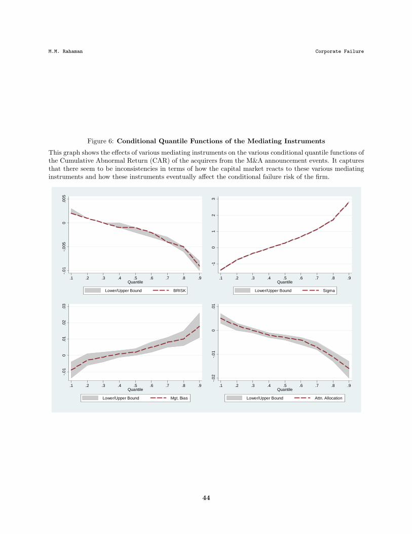
M.M. Rahaman Corporate Failure
Figure 6: Conditional Quantile Functions of the Mediating Instruments
This graph shows the effects of various mediating instruments on the various conditional quantile functions ofthe Cumulative Abnormal Return (CAR) of the acquirers from the M&A announcement events. It capturesthat there seem to be inconsistencies in terms of how the capital market reacts to these various mediatinginstruments and how these instruments eventually affect the conditional failure risk of the firm.
15
Figure 10: Effects of BRISK, Sigma, Mgt. Bias, and Attn. Allocation on Various Quantiles of the Conditional Distribution of Cumulative Abnormal Return (CAR) of Acquirers
-.01
-.005
0.0
05
.1 .2 .3 .4 .5 .6 .7 .8 .9Quantile
Lower/Upper Bound BRISK
-10
12
3
.1 .2 .3 .4 .5 .6 .7 .8 .9Quantile
Lower/Upper Bound Sigma
-.01
0.0
1.0
2.0
3
.1 .2 .3 .4 .5 .6 .7 .8 .9Quantile
Lower/Upper Bound Mgt. Bias
-.02
-.01
0.0
1
.1 .2 .3 .4 .5 .6 .7 .8 .9Quantile
Lower/Upper Bound Attn. Allocation
44
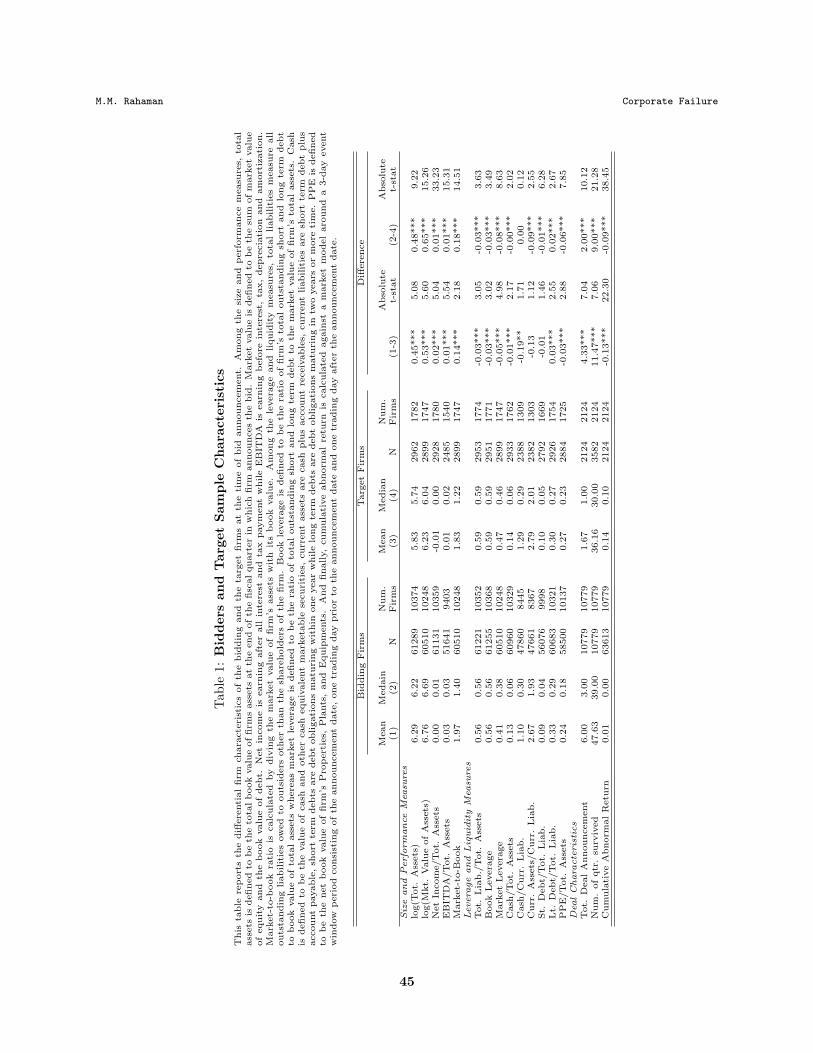
M.M. Rahaman Corporate Failure
Tab
le1:
Bid
der
san
dT
arge
tS
amp
leC
har
acte
rist
ics
This
table
rep
ort
sth
ediff
ere
nti
al
firm
chara
cte
rist
ics
of
the
bid
din
gand
the
targ
et
firm
sat
the
tim
eof
bid
announcem
ent.
Am
ong
the
size
and
perf
orm
ance
measu
res,
tota
lass
ets
isdefined
tob
eth
eto
tal
book
valu
eof
firm
sass
ets
at
the
end
of
the
fisc
al
quart
er
inw
hic
hfirm
announces
the
bid
.M
ark
et
valu
eis
defined
tob
eth
esu
mof
mark
et
valu
eof
equit
yand
the
book
valu
eof
debt.
Net
incom
eis
earn
ing
aft
er
all
inte
rest
and
tax
paym
ent
while
EB
ITD
Ais
earn
ing
befo
rein
tere
st,
tax,
depre
cia
tion
and
am
ort
izati
on.
Mark
et-
to-b
ook
rati
ois
calc
ula
ted
by
div
ing
the
mark
et
valu
eof
firm
’sass
ets
wit
hit
sb
ook
valu
e.
Am
ong
the
levera
ge
and
liquid
ity
measu
res,
tota
lliabilit
ies
measu
reall
outs
tandin
gliabilit
ies
ow
ed
toouts
iders
oth
er
than
the
share
hold
ers
of
the
firm
.B
ook
levera
ge
isdefined
tob
eth
era
tio
of
firm
’sto
tal
outs
tandin
gsh
ort
and
long
term
debt
tob
ook
valu
eof
tota
lass
ets
where
as
mark
et
levera
ge
isdefined
tob
eth
era
tio
of
tota
louts
tandin
gsh
ort
and
long
term
debt
toth
em
ark
et
valu
eof
firm
’sto
tal
ass
ets
.C
ash
isdefined
tob
eth
evalu
eof
cash
and
oth
er
cash
equiv
ale
nt
mark
eta
ble
securi
ties,
curr
ent
ass
ets
are
cash
plu
saccount
receiv
able
s,curr
ent
liabilit
ies
are
short
term
debt
plu
saccount
payable
,sh
ort
term
debts
are
debt
obligati
ons
matu
ring
wit
hin
one
year
while
long
term
debts
are
debt
obligati
ons
matu
ring
intw
oyears
or
more
tim
e.
PP
Eis
defined
tob
eth
enet
book
valu
eof
firm
’sP
rop
ert
ies,
Pla
nts
,and
Equip
ments
.A
nd
finally,
cum
ula
tive
abnorm
al
retu
rnis
calc
ula
ted
again
sta
mark
et
model
aro
und
a3-d
ay
event
win
dow
peri
od
consi
stin
gof
the
announcem
ent
date
,one
tradin
gday
pri
or
toth
eannouncem
ent
date
and
one
tradin
gday
aft
er
the
announcem
ent
date
.
Bid
din
gF
irm
sT
arg
et
Fir
ms
Diff
ere
nce
Mean
Medain
Num
.M
ean
Media
nN
um
.A
bso
lute
Abso
lute
(1)
(2)
NF
irm
s(3
)(4
)N
Fir
ms
(1-3
)t-
stat
(2-4
)t-
stat
Siz
eand
Perfo
rm
ance
Mea
sure
slo
g(T
ot.
Ass
ets
)6.2
96.2
261289
10374
5.8
35.7
42962
1782
0.4
5***
5.0
80.4
8***
9.2
2lo
g(M
kt.
Valu
eof
Ass
ets
)6.7
66.6
960510
10248
6.2
36.0
42899
1747
0.5
3***
5.6
00.6
5***
15.2
6N
et
Incom
e/T
ot.
Ass
ets
0.0
00.0
161131
10359
-0.0
10.0
02928
1780
0.0
2***
5.0
40.0
1***
33.2
3E
BIT
DA
/T
ot.
Ass
ets
0.0
30.0
351641
9403
0.0
10.0
22485
1540
0.0
1***
5.5
40.0
1***
15.3
1M
ark
et-
to-B
ook
1.9
71.4
060510
10248
1.8
31.2
22899
1747
0.1
4***
2.1
80.1
8***
14.5
1Levera
ge
and
Liq
uid
ity
Mea
sure
sT
ot.
Lia
b./
Tot.
Ass
ets
0.5
60.5
661221
10352
0.5
90.5
92953
1774
-0.0
3***
3.0
5-0
.03***
3.6
3B
ook
Levera
ge
0.5
60.5
661255
10368
0.5
90.5
92951
1771
-0.0
3***
3.0
2-0
.03***
3.4
9M
ark
et
Levera
ge
0.4
10.3
860510
10248
0.4
70.4
62899
1747
-0.0
5***
4.9
8-0
.08***
8.6
3C
ash
/T
ot.
Ass
ets
0.1
30.0
660960
10329
0.1
40.0
62933
1762
-0.0
1***
2.1
7-0
.00***
2.0
2C
ash
/C
urr
.L
iab.
1.1
00.3
047860
8445
1.2
90.2
92388
1309
-0.1
9**
1.7
10.0
00.1
2C
urr
.A
ssets
/C
urr
.L
iab.
2.6
71.9
347661
8367
2.7
92.0
12382
1303
-0.1
31.1
2-0
.09***
2.5
5St.
Debt/
Tot.
Lia
b.
0.0
90.0
456076
9998
0.1
00.0
52792
1669
-0.0
11.4
6-0
.01***
6.2
8L
t.D
ebt/
Tot.
Lia
b.
0.3
30.2
960683
10321
0.3
00.2
72926
1754
0.0
3***
2.5
50.0
2***
2.6
7P
PE
/T
ot.
Ass
ets
0.2
40.1
858500
10137
0.2
70.2
32884
1725
-0.0
3***
2.8
8-0
.06***
7.8
5D
ealChara
cte
ris
tics
Tot.
Deal
Announcem
ent
6.0
03.0
010779
10779
1.6
71.0
02124
2124
4.3
3***
7.0
42.0
0***
10.1
2N
um
.of
qtr
.su
rviv
ed
47.6
339.0
010779
10779
36.1
630.0
03582
2124
11.4
7***
7.0
69.0
0***
21.2
8C
um
ula
tive
Abnorm
al
Retu
rn0.0
10.0
063613
10779
0.1
40.1
02124
2124
-0.1
3***
22.3
0-0
.09***
38.4
5
45

M.M. Rahaman Corporate Failure
Tab
le2:
Exce
ssiv
ean
dC
onse
rvat
ive
Acq
uis
itiv
eS
amp
leC
har
acte
rist
ics
This
table
rep
ort
sth
ediff
ere
nti
al
firm
chara
cte
rist
ics
of
the
excess
ively
and
the
conse
rvati
vely
acquis
itiv
esa
mple
firm
sat
the
tim
eof
bid
announcem
ent.
Am
ong
the
size
and
perf
orm
ance
measu
res,
tota
lass
ets
isdefined
tob
eth
eto
tal
book
valu
eof
firm
sass
ets
at
the
end
of
the
fisc
al
quart
er
inw
hic
hfirm
announces
the
bid
.M
ark
et
valu
eis
defined
tob
eth
esu
mof
mark
et
valu
eof
equit
yand
the
book
valu
eof
debt.
Net
incom
eis
earn
ing
aft
er
all
inte
rest
and
tax
paym
ent
while
EB
ITD
Ais
earn
ing
befo
rein
tere
st,
tax,
depre
cia
tion
and
am
ort
izati
on.
Mark
et-
to-b
ook
rati
ois
calc
ula
ted
by
div
ing
the
mark
et
valu
eof
firm
’sass
ets
wit
hit
sb
ook
valu
e.
Am
ong
the
levera
ge
and
liquid
ity
measu
res,
tota
lliabilit
ies
measu
reall
outs
tandin
gliabilit
ies
ow
ed
toouts
iders
oth
er
than
the
share
hold
ers
of
the
firm
.B
ook
levera
ge
isdefined
tob
eth
era
tio
of
firm
’sto
tal
outs
tandin
gsh
ort
and
long
term
debt
tob
ook
valu
eof
tota
lass
ets
where
as
mark
et
levera
ge
isdefined
tob
eth
era
tio
of
tota
louts
tandin
gsh
ort
and
long
term
debt
toth
em
ark
et
valu
eof
firm
’sto
tal
ass
ets
.C
ash
isdefined
tob
eth
evalu
eof
cash
and
oth
er
cash
equiv
ale
nt
mark
eta
ble
securi
ties,
curr
ent
ass
ets
are
cash
plu
saccount
receiv
able
s,curr
ent
liabilit
ies
are
short
term
debt
plu
saccount
payable
,sh
ort
term
debts
are
debt
obligati
ons
matu
ring
wit
hin
one
year
while
long
term
debts
are
debt
obligati
ons
matu
ring
intw
oyears
or
more
tim
e.
PP
Eis
defined
tob
eth
enet
book
valu
eof
firm
’sP
rop
ert
ies,
Pla
nts
,and
Equip
ments
.A
nd
finally,
cum
ula
tive
abnorm
al
retu
rnis
calc
ula
ted
again
sta
mark
et
model
aro
und
a3-d
ay
event
win
dow
peri
od
consi
stin
gof
the
announcem
ent
date
,one
tradin
gday
pri
or
toth
eannouncem
ent
date
and
one
tradin
gday
aft
er
the
announcem
ent
date
.
Excess
ively
Acquis
itiv
eF
irm
sC
onse
rvati
vely
Acquis
itiv
eF
irm
sD
iffere
nce
Mean
Medain
Num
.M
ean
Media
nN
um
.A
bso
lute
Abso
lute
(1)
(2)
NF
irm
s(3
)(4
)N
Fir
ms
(1-3
)t-
stat
(2-4
)t-
stat
Siz
eand
Perfo
rm
ance
Mea
sure
slo
g(T
ot.
Ass
ets
)6.4
16.3
651630
8319
5.6
55.5
29630
5014
0.7
5***
14.2
70.8
4***
31.1
0lo
g(M
kt.
Valu
eof
Ass
ets
)6.8
86.8
351019
8227
6.1
26.0
29464
4925
0.7
6***
14.0
80.8
1***
26.5
9N
et
Incom
e/T
ot.
Ass
ets
0.0
00.0
151490
8303
0.0
00.0
19612
5008
0.0
0***
3.6
40.0
0***
8.2
6E
BIT
DA
/T
ot.
Ass
ets
0.0
30.0
343139
7462
0.0
20.0
38477
4514
0.0
1***
6.8
10.0
0***
10.6
6M
ark
et-
to-B
ook
1.9
41.4
051019
8227
2.1
21.3
99464
4925
-0.1
7***
4.0
00.0
2*
1.6
7Levera
ge
and
Liq
uid
ity
Mea
sure
sT
ot.
Lia
b./
Tot.
Ass
ets
0.5
60.5
651564
8297
0.5
40.5
39628
5013
0.0
3***
5.1
40.0
3***
9.2
7B
ook
Levera
ge
0.5
60.5
651597
8313
0.5
40.5
39629
5013
0.0
3***
5.1
70.0
3***
9.2
0M
ark
et
Levera
ge
0.4
20.3
851019
8227
0.4
00.3
59464
4925
0.0
2***
3.2
10.0
3***
6.0
6C
ash
/T
ot.
Ass
ets
0.1
20.0
551344
8275
0.1
60.0
79587
4997
-0.0
3***
10.4
9-0
.01***
10.6
5C
ash
/C
urr
.L
iab.
1.0
10.2
840175
6789
1.6
10.4
07656
3998
-0.6
1***
5.1
4-0
.11***
12.8
3C
urr
.A
ssets
/C
urr
.L
iab.
2.5
51.9
139977
6717
3.2
62.0
97655
3991
-0.7
1***
4.3
7-0
.18***
9.3
6St.
Debt/
Tot.
Lia
b.
0.0
90.0
447049
7998
0.0
80.0
38998
4767
0.0
1***
3.6
90.0
1***
8.8
5L
t.D
ebt/
Tot.
Lia
b.
0.3
30.3
051108
8273
0.2
80.2
19546
4983
0.0
5***
8.3
70.0
8***
14.9
5P
PE
/T
ot.
Ass
ets
0.2
40.1
749161
8116
0.2
30.1
59310
4858
0.0
1**
2.3
80.0
2***
7.3
5D
ealChara
cte
ris
tics
Cum
ula
tive
Abnorm
al
Retu
rn0.0
10.0
053494
8651
0.0
20.0
110087
5227
-0.0
1***
6.8
0-0
.01***
9.2
5
46

Tab
le3:
Wh
atD
rive
sF
irm
-Lev
elM
&A
Pro
pen
sity
?T
his
table
rep
ort
sth
eest
imate
sfr
om
am
ult
i-p
eri
od
logit
model
toasc
ert
ain
the
dete
rmin
ants
of
M&
Apro
pensi
tyof
the
sam
ple
firm
s.T
he
dep
endent
vari
able
inth
ere
gre
ssio
nis
1if
duri
ng
the
curr
ent
fisc
al
quart
er
firm
makes
an
M&
Abid
,oth
erw
ise
itit
0.
Tota
lass
ets
isdefined
tob
eth
eb
ook
valu
eof
firm
sass
ets
,net
incom
eis
incom
efr
om
op
era
tion
aft
er
all
taxes
and
inte
rest
paym
ent,
tota
lliabilit
ies
are
all
obligati
ons
due
toouts
iders
oth
er
than
the
share
hold
ers
of
the
firm
s,cash
are
the
valu
eof
cash
plu
soth
er
mark
eta
ble
securi
ties
hold
by
the
firm
,lo
ng
term
debts
are
debt
obligati
ons
due
intw
oor
more
years
tim
e,
PP
Eis
defined
tob
eth
enet
book
valu
eof
firm
’sP
lant,
Pro
pert
yand
Equip
ments
,and
mark
et
valu
eis
calc
ula
ted
as
mark
et
valu
eof
equit
yplu
sth
eb
ook
valu
eof
firm
’sdebt.
TF
Pst
ands
for
tota
lfa
cto
rpro
ducti
vit
yof
the
firm
est
imate
dfo
llow
ing
the
meth
odolo
gy
develo
ped
by
Olly
and
Pakes
(1996).
Indust
rycla
ssifi
cati
ons
are
base
don
Fam
a-F
rench
(1997).
We
use
the
tota
lin
dust
rynet
sale
sfr
om
the
quart
erl
yC
OM
PU
ST
AT
data
item
2as
pro
xy
for
indust
rydem
and
and
the
tota
lin
dust
rycost
of
good
sold
from
the
quart
erl
yC
OM
PU
ST
AT
data
item
30
as
pro
xy
for
indust
rysu
pply
.W
eals
ocollect
info
rmati
on
ab
out
all
pate
nts
for
the
peri
od
of
1963-2
002
from
the
NB
ER
pate
nt
data
base
and
convert
the
ass
igned
tech
nolo
gy
cla
ssof
each
of
those
pate
nts
into
inte
rnati
onal
pate
nt
cla
ssusi
ng
the
meth
odolo
gy
develo
ped
by
Silverm
an
(2002).
Fro
mth
ein
tern
ati
onal
pate
nt
cla
ssw
ecovert
them
back
into
1987
Sta
ndard
Indust
ryC
lass
ificati
ons
and
ass
ign
the
pate
nts
by
gra
nt
year
toeach
of
our
49
Fam
aand
Fre
nch
(1997)
indust
ries.
We
then
decom
pose
the
seri
es
into
trend
and
irre
gula
rcom
ponents
usi
ng
the
Hodri
ck-P
resc
ott
(HP
)filt
er.
Aft
er
decom
posi
ng
the
trend
and
irre
gula
rcom
ponents
of
the
seri
es,
we
calc
ula
tese
ries
inst
abilit
yby
est
imati
ng
the
accele
rati
on
(change
of
change)
of
the
irre
gula
rcom
ponent.
We
use
majo
rdere
gula
tory
init
iati
ves
duri
ng
the
sam
ple
peri
od
as
apro
xy
for
regula
tory
shock
s.W
euse
the
quart
erl
yre
al
GD
Pdata
from
the
Federa
lR
ese
rve
Bank
of
St.
Louis
as
pro
xy
for
aggre
gate
dem
and
and
the
real
pri
ce
of
cru
de
petr
ole
um
inth
eU
.S.
from
the
U.S
.E
nerg
yIn
form
ati
on
Adm
inis
trati
on
as
apro
xy
for
aggre
gate
supply
.U
tilizin
gth
eH
Pfilt
er,
we
then
calc
ula
teth
eaggre
gate
dem
and
and
supply
shock
.A
sa
pro
xy
for
aggre
gate
equit
yand
debt
mark
et
inst
abilit
yw
eapply
the
HP
filt
er
on
the
Dow
Jones
Indust
rial
avera
ge
and
bank
pri
me
lendin
gra
te,
resp
ecti
vely
.T
ocaptu
reth
em
om
entu
min
equit
ym
ark
et,
we
apply
the
HP
filt
er
on
S&
P500
index
and
use
the
smooth
ed
trend
port
ion
of
seri
es
as
our
pro
xy
for
mom
entu
min
aggre
gate
equit
ym
ark
et.
We
als
oconst
ruct
measu
res
of
indust
rym
erg
er
wave
uti
lizin
gth
eX
-12-A
RIM
A,
ase
aso
nal
adju
stm
ent
soft
ware
pro
duced
and
main
tain
ed
by
the
U.S
.C
ensu
sB
ure
au.
We
deta
ilth
econst
ructi
on
of
all
vari
able
sin
the
data
secti
on
of
the
pap
er.
Robust
zst
ati
stic
sare
giv
en
inbra
ckets
and
“*”
denote
ssi
gnifi
cance
at
10%
;“**”
denote
ssi
gnifi
cance
at
5%
;“***”
denote
ssi
gnifi
cance
at
1%
level.
(1)
(2)
(3)
(4)
(5)
(6)
(7)
(8)
(9)
(10)
(11)
(12)
(13)
(14)
log(T
ot.
Ass
ets
)0.2
631***
0.2
614***
0.2
635***
0.2
637***
0.2
634***
0.2
786***
0.2
617***
0.2
632***
0.2
636***
0.2
635***
0.2
631***
0.2
396***
0.2
514***
0.2
719***
[36.5
1]
[32.9
3]
[36.5
5]
[36.0
3]
[36.0
5]
[33.9
8]
[36.2
8]
[36.5
1]
[36.5
6]
[36.5
6]
[36.5
1]
[31.4
6]
[28.7
0]
[31.0
6]
Net
Incom
e/T
ot.
Ass
ets
0.4
299**
0.6
827***
0.4
271**
0.4
706**
0.4
706**
0.4
821***
0.4
624**
0.4
301**
0.4
215**
0.4
179**
0.4
295**
0.6
756***
0.8
449***
0.5
530***
[2.4
1]
[4.6
1]
[2.3
9]
[2.4
1]
[2.4
1]
[3.5
5]
[2.4
4]
[2.4
0]
[2.4
1]
[2.4
1]
[2.4
0]
[3.2
8]
[6.0
6]
[3.7
0]
Tot.
Lia
b./
Tot.
Ass
ets
-0.9
870***
-1.0
775***
-0.9
891***
-0.9
895***
-0.9
887***
-0.9
453***
-0.9
894***
-0.9
871***
-0.9
884***
-0.9
874***
-0.9
870***
-0.9
316***
-0.9
159***
-0.9
535***
[15.4
7]
[14.9
7]
[15.4
9]
[15.3
6]
[15.3
5]
[13.4
4]
[15.5
4]
[15.4
7]
[15.5
0]
[15.4
9]
[15.4
7]
[14.9
5]
[13.6
2]
[13.9
3]
Cash
/T
ot.
Ass
ets
-0.2
880***
-0.1
547**
-0.2
890***
-0.2
954***
-0.2
966***
-0.1
492*
-0.3
023***
-0.2
884***
-0.2
886***
-0.2
875***
-0.2
883***
-0.2
856***
-0.2
051***
-0.1
406*
[3.9
7]
[2.1
7]
[3.9
9]
[4.0
4]
[4.0
6]
[1.9
2]
[4.1
8]
[3.9
8]
[3.9
8]
[3.9
7]
[3.9
8]
[3.9
7]
[2.7
2]
[1.8
7]
Lt.
Debt/
Tot.
Ass
ets
0.6
680***
0.8
049***
0.6
699***
0.6
666***
0.6
668***
0.7
279***
0.6
633***
0.6
681***
0.6
673***
0.6
672***
0.6
679***
0.6
238***
0.6
794***
0.6
836***
[11.7
2]
[12.5
8]
[11.7
6]
[11.6
1]
[11.6
2]
[11.5
1]
[11.6
7]
[11.7
2]
[11.7
1]
[11.7
1]
[11.7
2]
[11.1
5]
[10.9
7]
[11.2
2]
PP
E/T
ot.
Ass
ets
-1.0
641***
-1.1
801***
-1.0
646***
-1.0
639***
-1.0
634***
-1.1
931***
-1.0
324***
-1.0
645***
-1.0
659***
-1.0
654***
-1.0
641***
-0.8
517***
-0.9
347***
-0.9
713***
[12.4
4]
[12.9
8]
[12.4
5]
[12.3
6]
[12.3
4]
[12.6
3]
[12.1
1]
[12.4
4]
[12.4
5]
[12.4
5]
[12.4
4]
[10.0
5]
[10.1
2]
[10.6
1]
Mark
et-
to-B
ook
0.0
434***
0.0
434***
0.0
434***
0.0
434***
0.0
394***
0.0
413***
0.0
434***
0.0
430***
0.0
430***
0.0
434***
0.0
382***
0.0
294***
0.0
264***
[5.2
0]
[5.2
1]
[5.1
6]
[5.1
6]
[4.6
6]
[5.0
2]
[5.2
0]
[5.1
6]
[5.1
7]
[5.2
0]
[4.7
5]
[3.9
8]
[3.5
8]
Change
inT
FP
0.0
773***
[3.0
7]
Dere
gula
tion
Dum
my
0.1
554***
0.1
887***
0.1
036*
[4.2
5]
[2.9
7]
[1.6
7]
Ind.
Dem
and
Shock
-0.0
001***
-0.0
001*
-0.0
000
[4.6
4]
[1.7
2]
[0.0
6]
Ind.
Supply
Shock
-0.0
002***
-0.0
001
-0.0
002
[2.8
1]
[0.5
6]
[1.5
9]
Ind.
Tech
.Shock
0.0
525***
0.0
523***
0.0
185**
[6.7
0]
[6.5
4]
[2.3
1]
Ind.
Merg
er
Wave
Dum
my
0.1
070***
0.2
155***
0.1
036***
[5.9
8]
[9.6
9]
[4.5
8]
Agg.
Dem
and
Shock
0.2
396***
0.3
173***
0.0
485
[3.1
9]
[3.6
4]
[0.4
9]
Agg.
Supply
Shock
2.4
408***
3.6
973***
2.9
368***
[5.8
2]
[5.5
4]
[3.6
1]
Agg.
Equit
yShock
-0.0
569***
-0.1
177***
0.0
035
[5.6
5]
[10.9
2]
[0.2
3]
Agg.
Debt
Shock
0.0
096***
0.0
007
0.0
078
[4.1
0]
[0.1
8]
[1.2
3]
Agg.
Equit
yM
om
entu
m0.2
982***
0.3
636***
6.3
454***
[21.1
3]
[22.5
8]
[33.0
4]
Const
ant
-2.9
692***
-2.8
365***
-2.9
706***
-2.9
584***
-2.9
589***
-2.9
925***
-2.9
105***
-2.9
694***
-2.9
684***
-2.9
667***
-2.9
692***
-4.8
050***
-5.1
432***
-34.6
772***
[11.1
4]
[10.3
5]
[11.1
4]
[11.0
4]
[11.0
5]
[10.7
4]
[10.9
9]
[11.1
4]
[11.1
3]
[11.1
3]
[11.1
4]
[17.7
5]
[18.4
5]
[34.7
9]
Ind.
Fix
ed
Eff
ect
Yes
Yes
Yes
Yes
Yes
Yes
Yes
Yes
Yes
Yes
Yes
Yes
Yes
Yes
Year
Fix
ed
Eff
ect
No
No
No
No
No
No
No
No
No
No
No
No
No
Yes
N418346
354539
418346
415000
415259
326968
410347
418346
418346
418346
418346
418346
316753
316728
Num
.of
Fir
ms
10439
8923
10439
10355
10356
8759
10439
10439
10439
10439
10439
10439
8677
8677
Pse
udo-R
20.0
60.0
60.0
60.0
60.0
60.0
60.0
60.0
60.0
60.0
60.0
60.0
60.0
70.0
9W
ald
-χ2
2375.9
02179.2
32378.9
52374.0
82357.0
42109.2
62369.9
92382.6
72391.6
42401.9
82385.4
13438.5
33161.4
54562.3
4
47

Table 4: What Drives Firm-Level M&A Propensity? Decomposition of the Economic ShocksThis table decomposes the economic shocks into positive and negative components and reports the estimates from a multi-period logitmodel. The dependent variable in the regression is 1 if during the current fiscal quarter firm makes an M&A bid, otherwise it is 0. Totalassets is defined to be the book value of firms assets, net income is income from operation after all taxes and interest payment, totalliabilities are all obligations due to outsiders other than the shareholders of the firms, cash are the value of cash plus other marketablesecurities hold by the firm, long term debts are debt obligations due in two or more years time, PPE is defined to be the net book valueof firm’s Plant, Property and Equipments, and market value is calculated as market value of equity plus the book value of firm’s debt.TFP stands for total factor productivity of the firm estimated following the methodology developed by Olly and Pakes (1996). Industryclassifications are based on Fama-French (1997). We use the total industry net sales from the quarterly COMPUSTAT data item 2 asproxy for industry demand and the total industry cost of good sold from the quarterly COMPUSTAT data item 30 as proxy for industrysupply. We also collect information about all patents for the period of 1963-2002 from the NBER patent database and convert theassigned technology class of each of those patents into international patent class using the methodology developed by Silverman (2002).From the international patent class we covert them back into 1987 Standard Industry Classifications and assign the patents by grantyear to each of our 49 Fama and French (1997) industries. We then decompose the series into trend and irregular components usingthe Hodrick-Prescott (HP) filter. After decomposing the trend and irregular components of the series, we calculate series instability byestimating the acceleration (change of change) of the irregular component. We use major deregulatory initiatives during the sampleperiod as a proxy for regulatory shocks. We use the quarterly real GDP data from the Federal Reserve Bank of St. Louis as proxy foraggregate demand and the real price of crude petroleum in the U.S. from the U.S. Energy Information Administration as a proxy foraggregate supply. Utilizing the HP filter, we then calculate the aggregate demand and supply shock. As a proxy for aggregate equityand debt market instability we apply the HP filter on the Dow Jones Industrial average and bank prime lending rate, respectively. Ifthe actual series has been above the HP filtered trend components for at least three consecutive periods then we treat the shock aspositive and if the actual series has been below the trend components for three consecutive periods then we treat the shock as negative.To capture the momentum in equity market, we apply the HP filter on S&P 500 index and use the smoothed trend portion of series asour proxy for momentum in aggregate equity market. We also construct measures of industry merger wave utilizing the X-12-ARIMA,a seasonal adjustment software produced and maintained by the U.S. Census Bureau. We detail the construction of all variables in thedata section of the paper. Robust z statistics are given in brackets and “*” denotes significance at 10%; “**” denotes significance at5%; “***” denotes significance at 1% level.
(1) (2) (3) (4) (5) (6) (7) (8) (9)
log(Tot. Assets) 0.2627*** 0.2632*** 0.2784*** 0.2633*** 0.2645*** 0.2638*** 0.2631*** 0.2509*** 0.2708***[36.16] [36.06] [34.02] [36.51] [36.46] [36.54] [36.49] [28.89] [31.24]
Net Income/Tot. Assets 0.4713** 0.4704** 0.4803*** 0.4307** 0.4236** 0.4218** 0.4269** 0.8438*** 0.5435***[2.42] [2.41] [3.54] [2.41] [2.40] [2.40] [2.41] [6.15] [3.66]
Tot. Liab./Tot. Assets -0.9831*** -0.9893*** -0.9451*** -0.9874*** -0.9905*** -0.9872*** -0.9878*** -0.9123*** -0.9483***[15.39] [15.37] [13.44] [15.48] [15.51] [15.48] [15.48] [13.71] [14.00]
Cash/Tot. Assets -0.2949*** -0.2965*** -0.1486* -0.2882*** -0.2854*** -0.2853*** -0.2879*** -0.1997*** -0.1453*[4.08] [4.06] [1.92] [3.97] [3.93] [3.94] [3.97] [2.68] [1.96]
Lt. Debt/Tot. Assets 0.6588*** 0.6668*** 0.7276*** 0.6686*** 0.6668*** 0.6664*** 0.6681*** 0.6726*** 0.6750***[11.63] [11.63] [11.50] [11.73] [11.69] [11.70] [11.73] [11.03] [11.25]
PPE/Tot. Assets -1.0480*** -1.0618*** -1.1924*** -1.0647*** -1.0705*** -1.0665*** -1.0627*** -0.9223*** -0.9546***[12.36] [12.32] [12.63] [12.44] [12.45] [12.46] [12.42] [10.16] [10.58]
Market-to-Book 0.0426*** 0.0432*** 0.0391*** 0.0435*** 0.0430*** 0.0427*** 0.0433*** 0.0288*** 0.0258***[5.11] [5.15] [4.64] [5.21] [5.16] [5.14] [5.19] [3.98] [3.57]
Pos. Ind. Demand Shock 0.0033*** 0.0027*** 0.0030***[9.27] [7.09] [8.31]
Neg. Ind. Demane Shock -0.0018*** -0.0022*** -0.0014***[5.51] [5.00] [3.14]
Pos. Ind. Supply Shock 0.0022** 0.0042*** 0.0042***[2.17] [3.03] [2.97]
Neg. Ind. Supply Shock -0.0010 0.0004 0.0013[0.91] [0.41] [1.21]
Pos. Ind. Tech. Shock -0.0052 0.0354*** 0.0486***[0.36] [2.63] [3.56]
Neg. Ind. Tech. Shock 0.0020 0.0476** 0.0057[0.10] [2.05] [0.23]
Pos. Agg. Demand Shock 0.5565*** 0.1588 0.1491[5.08] [1.43] [1.17]
Neg. Agg. Demand Shock 0.0105 -0.1019 0.0281[0.07] [0.43] [0.12]
Pos. Agg. Supply Shock -0.7101 -3.1745** 13.7910***[0.60] [2.09] [6.64]
Neg. Agg. Supply Shock 9.2105*** 4.8126*** 1.4380[11.52] [4.86] [1.24]
Pos. Agg. Equity Shock -0.0732*** -0.0292* 0.0097[4.23] [1.83] [0.53]
Neg. Agg. Equity Shock -0.1249*** -0.3047*** 0.6126***[5.56] [11.46] [8.89]
Pos. Agg. Debt Shock 0.0107* 0.0384*** 0.0554***[1.69] [4.75] [5.00]
Neg. Agg. Debt Shock -0.1104*** -0.1216*** -0.1296***[6.94] [6.28] [5.66]
Deregulation Dummy 0.2054*** 0.0923[3.28] [1.50]
Ind Merger Wave Dummy 0.2164*** 0.1038***[9.85] [4.65]
Agg. Equity Momentum 0.3537*** 6.5266***[22.00] [33.94]
Constant -2.9636*** -2.9601*** -2.9913*** -2.9695*** -2.9804*** -2.9665*** -2.9627*** -5.0925*** -35.5046***[11.23] [11.12] [10.74] [11.14] [11.16] [11.14] [11.12] [18.81] [35.67]
Ind. Fixed Effect Yes Yes Yes Yes Yes Yes Yes Yes YesYear Fixed Effect No No No No No No No No YesN 415000 415259 326968 418346 418346 418346 418346 316753 316728Num. of Firms 10355 10356 8759 10439 10439 10439 10439 8677 8677Pseudo-R2 0.06 0.06 0.06 0.06 0.06 0.06 0.06 0.07 0.09Wald-χ2 2417.18 2350.48 2068.55 2388.21 2544.65 2451.05 2444.72 3184.62 4989.05
48

M.M. Rahaman Corporate Failure
Table 5: Why Some Firms Are More Acquisitive Than Others?This table shows the correlation structure of managerial acquisitiveness with firm’s productivity shocks, investment and acquisitionexpenditure, future growth opportunity, and governance proxies. We discuss the construction of the excessive acquisitiveness measurein detail in the data section of the paper. TFP stands for total factor productivity estimated using the methodology developed by Ollyand Pakes (1996). Optimism driven bid is a dummy variable which equals 1 if the firm announces an acquisition bid even if it receivesa negative productivity shock in that period while growth driven bid is another dummy variable which equals 1 if the firm announcesan acquisition bid when market-to-book ratio is greater than 1. Firm level capital expenditure and acquisition expenditure are fromCOMPUSTAT data item 90 and data item 94, respectively. Governance index (G) is from Gompers, Ishii and Metrick (2003). P-valuesare given in bracket
Managerial Acquistiveness
Excessive Acq. Sample Non-Excessive Acq. Sample
Change in TFP 0.00670 -0.00550[0.00] [0.00]
Optimism Driven Bid 0.13160 -0.07300[0.00] [0.00]
Growth Driven Bid 0.28210 -0.14650[0.00] [0.00]
Capital Expenditure 0.07090 -0.00580[0.00] [0.00]
Acquisition Expenditure 0.10220 -0.01450[0.00] [0.00]
Acquirer’s G-Index 0.04680 -0.02690[0.00] [0.00]
49

M.M. Rahaman Corporate Failure
Tab
le6:
Exce
ssiv
eU
seof
M&
AIn
vest
men
tT
ech
nol
ogy
and
Cor
por
ate
Fai
lure
This
table
rep
ort
sth
eest
imate
sfr
om
adis
cre
te-t
ime
hazard
model
todete
rmin
eth
eeff
ect
of
manageri
al
acquis
itiv
eness
on
firm
’sfa
ilure
hazard
.T
he
dep
endent
vari
able
inth
ere
gre
ssio
nis
1fo
rth
ep
eri
od
inw
hic
hth
efirm
fails
and
0oth
erw
ise.
The
definit
ions
of
all
the
expla
nato
ryvari
able
sare
sam
eas
inth
epre
vio
us
table
s.T
he
Dis
tance
toN
atu
ral
Hedge
vari
able
isconst
ructe
dusi
ng
the
equati
on
2in
the
pap
er.
Robust
zst
ati
stic
sare
giv
en
inbra
ckets
and
“*”
denote
ssi
gnifi
cance
at
10%
;“**”
denote
ssi
gnifi
cance
at
5%
;“***”
denote
ssi
gnifi
cance
at
1%
level.
(1)
(2)
(3)
(4)
(5)
(6)
(7)
(8)
(9)
(10)
(11)
(12)
log(T
ot.
Ass
ets
)-0
.4945**
-0.5
728***
-0.5
916***
-1.5
172***
-0.4
15***
-0.5
104***
-0.4
993*
-0.5
806**
-0.6
098**
-1.1
919***
-0.3
72***
-0.4
927***
[2.3
3]
[2.9
3]
[2.9
2]
[4.9
7]
[6.2
5]
[7.5
1]
[1.9
1]
[2.3
2]
[2.3
6]
[5.0
1]
[5.1
7]
[6.6
9]
log(A
ge)
-0.6
399***
-0.5
057***
-0.4
664***
-0.4
324***
-0.7
84***
-0.7
445***
-0.6
113***
-0.4
342***
-0.4
150***
-0.3
733***
-0.7
51***
-0.6
957***
[6.9
8]
[6.1
8]
[5.8
7]
[3.2
3]
[6.1
5]
[5.5
0]
[5.3
7]
[4.0
4]
[3.8
3]
[2.8
1]
[5.3
0]
[4.4
8]
Net
Incom
e/T
ot.
Ass
ets
-0.2
080***
-0.3
289
-0.1
456***
0.8
086*
-0.8
91***
-0.8
620***
-0.5
216*
-1.1
425*
-0.1
365**
0.2
000
-0.7
04***
-0.6
623**
[2.9
6]
[0.8
1]
[3.1
8]
[1.8
8]
[3.6
1]
[3.5
6]
[1.9
3]
[1.9
4]
[2.3
0]
[1.0
0]
[2.8
7]
[2.5
4]
Tot.
Lia
b./
Tot.
Ass
ets
0.9
312
0.9
249***
0.9
232
1.4
626**
3.2
12***
3.1
509***
0.6
704
0.6
979
0.7
856
1.0
252***
3.6
71***
3.5
406***
[1.4
4]
[2.9
0]
[1.6
2]
[2.1
0]
[11.8
7]
[11.9
5]
[0.7
1]
[0.7
4]
[1.2
7]
[8.6
9]
[10.4
0]
[10.3
0]
Cash
/T
ot.
Ass
ets
-0.6
792
-0.3
066
-0.1
813
3.9
651***
0.4
72
0.8
115*
-1.3
080
-0.7
847
-0.6
743
1.8
604*
-0.2
01
0.1
631
[0.7
5]
[0.3
4]
[0.2
1]
[3.1
7]
[0.9
9]
[1.6
9]
[1.1
1]
[0.7
4]
[0.5
7]
[1.9
5]
[0.3
6]
[0.2
9]
Lt.
Debt/
Tot.
Ass
ets
-0.4
256
-0.5
097
-0.6
270
-0.1
513
-1.8
00***
-1.9
001***
-0.3
927
-0.4
458
-0.7
121
-0.0
523
-1.9
35***
-2.0
571***
[0.0
8]
[0.1
0]
[0.1
2]
[0.9
1]
[4.6
1]
[4.8
4]
[0.0
6]
[0.0
7]
[0.1
1]
[0.8
5]
[4.4
2]
[4.6
5]
PP
E/T
ot.
Ass
ets
0.1
388
0.3
889
0.5
073
1.6
802***
1.2
21**
1.5
018***
0.1
537
0.3
913
0.5
790
2.0
648***
1.4
34***
1.6
752***
[0.0
8]
[0.2
2]
[0.2
9]
[2.8
7]
[2.4
2]
[2.8
7]
[0.0
7]
[0.2
0]
[0.2
8]
[2.9
7]
[2.6
3]
[2.8
9]
Mark
et-
to-B
ook
-0.5
918***
-0.7
134***
-0.5
964***
-0.7
501***
-1.9
68***
-1.9
471***
-0.5
522***
-0.5
586***
-0.5
551***
-0.7
435***
-2.0
82***
-2.0
458***
[3.4
0]
[4.0
5]
[3.4
3]
[5.3
4]
[7.7
6]
[7.9
2]
[3.0
7]
[3.2
1]
[2.6
2]
[9.6
8]
[6.3
8]
[6.5
0]
Dis
tance
toN
.H
edge
2.9
351***
3.1
055***
[5.5
9]
[5.1
1]
Excess
ive
Acq.
3.1
217***
1.9
575***
3.3
286***
2.3
355***
[6.2
1]
[7.5
3]
[5.1
6]
[8.4
9]
Excess
ive
Acq.
IV48.4
192***
28.1
494***
[3.4
9]
[2.8
0]
Govern
ance
Score
-0.0
33
-0.0
297
-0.0
28
-0.0
232
[1.0
6]
[0.9
5]
[0.7
8]
[0.6
3]
Dere
gula
tion
Dum
my
-0.2
395
-0.2
242
-0.2
085
0.1
748
0.7
44
0.8
799
[1.1
0]
[1.0
2]
[0.9
7]
[0.6
3]
[0.9
3]
[1.0
9]
Ind.
Dem
and
Shock
0.0
005**
0.0
006**
0.0
005**
0.0
008***
0.0
00
0.0
003
[2.2
8]
[2.5
3]
[2.5
6]
[3.3
9]
[0.3
7]
[0.4
1]
Ind.
Supply
Shock
-0.0
005
-0.0
006
-0.0
006
-0.0
007
-0.0
00
-0.0
001
[1.3
1]
[1.5
1]
[1.3
8]
[1.5
3]
[0.0
7]
[0.0
6]
Ind.
Tech
.Shock
0.0
336
0.0
395
0.0
352
0.0
473*
0.0
75
0.0
669
[1.0
9]
[1.3
2]
[1.1
6]
[1.8
6]
[0.9
0]
[0.8
0]
Agg.
Dem
and
Shock
1.1
507***
1.2
745***
1.1
733***
0.7
867*
-0.2
97*
1.3
913
[2.8
4]
[3.1
7]
[2.9
0]
[1.8
0]
[1.8
1]
[0.9
7]
Agg.
Supply
Shock
0.9
461
1.8
302
1.2
174
-1.1
690
1.3
45
-29.0
461*
[0.3
1]
[0.6
2]
[0.4
0]
[0.4
5]
[0.9
7]
[1.9
2]
Agg.
Equit
yShock
-0.1
523***
-0.1
329**
-0.1
339***
-0.0
687
-29.3
37**
-0.2
876*
[3.0
7]
[2.5
6]
[2.6
1]
[1.2
0]
[1.9
6]
[1.7
3]
Agg.
Debt
Shock
-0.0
535
-0.0
547
-0.0
434
-0.0
458*
0.0
66
0.0
502
[1.3
8]
[1.2
8]
[1.1
5]
[1.6
8]
[0.3
3]
[0.2
5]
Agg.
Equit
yM
om
entu
m1.2
905
0.8
935
1.0
292
1.0
019***
0.1
97
0.2
466
[1.5
3]
[0.9
8]
[1.2
4]
[14.8
7]
[0.0
9]
[0.1
1]
Const
ant
-2.1
960**
-4.8
474***
-3.3
751***
-1.1
064
-13.2
03***
-13.4
186***
-8.1
319**
-8.7
534**
-7.9
488**
-7.3
653***
-14.4
51
-13.6
694
[2.4
4]
[5.7
3]
[4.2
7]
[1.1
9]
[10.2
7]
[10.5
8]
[2.2
6]
[2.1
2]
[2.2
1]
[12.6
6]
[0.9
0]
[.]
Ind.
Dum
my
Yes
Yes
Yes
No
Yes
Yes
Yes
Yes
Yes
No
Yes
Yes
Year
Dum
my
Yes
Yes
Yes
No
Yes
Yes
Yes
Yes
Yes
No
Yes
Yes
N412416
408589
408589
409080
127394
125861
318928
315595
315595
315740
94806
93554
Num
.of
Fir
ms
10439
10439
10439
2661
2658
8678
8678.0
08678
2341
2337
Pse
udo-R
20.1
40.1
70.1
80.2
1.2
20.1
40.1
70.1
90.2
30.2
5W
ald
-Chi2
9803.8
17436.5
65624.4
29213.4
96908.8
95109.6
2
50

M.M. Rahaman Corporate Failure
Tab
le7:
Exce
ssiv
eU
seof
M&
AIn
vest
men
tT
ech
nol
ogy
and
Cor
por
ate
Fai
lure
:R
obu
stn
ess
Tes
tsT
his
table
rep
ort
sth
ero
bust
ness
test
sof
the
causa
leff
ects
of
excess
ive
acquis
itiv
eness
on
firm
failure
.D
efinit
ions
of
all
the
vari
able
sare
sam
eas
inth
epre
vio
us
table
s.W
em
easu
reconse
rvati
ve
acquis
itiv
eness
usi
ngCONSERV
ACQijt
=DIST.NHijt×I(Xijt−Median(X−ijT
)<0).
To
measu
rewinner,
we
use
cum
ula
tive
num
ber
of
com
ple
ted
conte
sted
bid
snorm
alized
by
the
tota
lnum
ber
of
deals
com
ple
ted
by
the
firm
.R
obust
zst
ati
stic
sare
giv
en
inbra
ckets
and
“*”
denote
ssi
gnifi
cance
at
10%
;“**”
denote
ssi
gnifi
cance
at
5%
;“***”
denote
ssi
gnifi
cance
at
1%
level.
(1)
(2)
(3)
(4)
(5)
(6)
(7)
(8)
(9)
(10)
Non-l
ineari
tyL
inear
Pro
babilit
yM
odel
Focusi
ng
on
the
1980s
Win
ners
’C
urs
eT
wo
Dim
ensi
onal
Clu
steri
ng
wit
hfirm
FE
sam
ple
only
Expla
nati
on
(by
firm
and
size)
log(T
ot.
Ass
ets
)-0
.5653***
-0.5
604**
-0.0
101***
-0.0
110***
-0.5
300***
-0.5
297***
-0.5
933***
-0.6
114**
-0.5
737***
-0.5
488**
[2.5
8]
[2.0
6]
[25.2
2]
[23.8
2]
[30.3
9]
[27.4
6]
[2.9
2]
[2.3
6]
[2.6
7]
[2.3
1]
log(A
ge)
-0.6
191***
-0.5
713***
0.0
346***
0.0
469***
-0.4
610***
-0.3
947***
-0.4
664***
-0.4
151***
-0.5
586***
-0.4
490***
[6.6
2]
[4.7
2]
[31.4
8]
[27.8
0]
[10.9
0]
[8.3
9]
[5.8
4]
[3.8
1]
[5.1
8]
[3.4
3]
Net
Incom
e/T
ot.
Ass
ets
-0.2
722
-1.0
614*
0.0
012
0.0
014
-0.0
977*
-0.1
031***
-0.1
457***
-0.1
369**
-0.2
832
0.0
667
[0.7
7]
[1.7
5]
[0.9
4]
[1.0
5]
[1.7
5]
[3.2
1]
[3.1
6]
[2.2
7]
[0.6
2]
[0.1
7]
Tot.
Lia
b./
Tot.
Ass
ets
1.0
557*
0.8
300
0.0
041
0.0
036
1.6
296***
1.6
775***
0.9
232
0.7
858
0.7
771
0.5
609
[1.8
9]
[0.8
0]
[1.4
5]
[1.4
4]
[13.1
9]
[13.9
1]
[1.6
3]
[1.2
7]
[1.1
9]
[0.9
2]
Cash
/T
ot.
Ass
ets
-0.2
657
-0.7
880
-0.0
148***
-0.0
151***
0.2
150
-0.1
810
-0.1
801
-0.6
747
-0.1
572
-0.7
490
[0.2
9]
[0.7
3]
[7.2
5]
[7.1
0]
[1.3
8]
[1.0
0]
[0.2
1]
[0.5
8]
[0.1
8]
[0.6
3]
Lt.
Debt/
Tot.
Ass
ets
-0.5
757
-0.5
341
-0.0
002
-0.0
001
-0.9
990***
-1.1
863***
-0.6
234
-0.7
110
-0.4
360
-0.4
633
[0.1
1]
[0.0
9]
[0.8
7]
[0.7
8]
[8.5
7]
[9.3
6]
[0.1
2]
[0.1
1]
[0.0
8]
[0.0
8]
PP
E/T
ot.
Ass
ets
0.3
842
0.3
939
0.0
043*
0.0
069***
0.6
663***
0.7
475***
0.5
135
0.5
879
0.4
242
0.4
312
[0.2
1]
[0.1
9]
[1.9
0]
[2.6
3]
[4.9
2]
[5.0
3]
[0.2
9]
[0.2
8]
[0.2
1]
[0.2
1]
Mark
et-
to-B
ook
-0.6
813***
-0.6
043***
-0.0
008***
-0.0
007**
-0.5
927***
-0.5
361***
-0.5
971***
-0.5
563***
-0.6
389***
-0.3
526**
[3.3
0]
[2.9
6]
[2.6
7]
[2.5
4]
[8.6
9]
[7.1
8]
[3.4
4]
[2.6
3]
[3.9
6]
[1.9
7]
Conse
rvA
cq.
-19.4
124***
-21.8
251***
[10.7
4]
[13.1
4]
Excess
ive
Acq.
0.0
314***
0.0
351***
3.0
707***
3.2
698***
3.1
102***
3.3
168***
3.0
461***
3.1
429***
[18.3
9]
[17.4
0]
[34.0
6]
[33.6
4]
[6.1
5]
[5.1
2]
[4.9
6]
[4.6
8]
Win
ner
2.3
251***
2.2
976***
[5.5
1]
[4.3
9]
Dere
gula
tion
Dum
my
-0.2
621
-0.0
018*
0.0
318
-0.2
051
-0.2
623
[1.0
7]
[1.9
2]
[0.1
5]
[0.9
5]
[1.2
3]
Ind.
Dem
and
Shock
0.0
005**
0.0
000***
0.0
005**
0.0
006***
0.0
006***
[2.4
2]
[3.1
4]
[2.1
6]
[2.6
4]
[3.3
8]
Ind.
Supply
Shock
-0.0
006
-0.0
000
-0.0
005
-0.0
006
-0.0
008*
[1.3
5]
[1.6
3]
[1.1
1]
[1.4
3]
[1.8
8]
Ind.
Tech
.Shock
0.0
290
0.0
002
0.0
240
0.0
350
0.0
418
[0.9
1]
[1.4
7]
[0.7
1]
[1.1
5]
[1.3
9]
Agg.
Dem
and
Shock
1.0
830***
0.0
086***
1.3
199***
1.1
264***
1.3
457***
[2.6
2]
[2.7
1]
[2.8
9]
[2.7
8]
[3.6
8]
Agg.
Supply
Shock
0.2
183
0.0
145
-0.5
887
1.3
826
0.9
994
[0.0
7]
[0.7
9]
[0.1
6]
[0.4
5]
[0.3
5]
Agg.
Equit
yShock
-0.1
594***
-0.0
010**
-0.1
219**
-0.1
319***
-0.1
401***
[3.0
5]
[2.0
2]
[2.2
3]
[2.5
8]
[3.2
0]
Agg.
Debt
Shock
-0.0
524
-0.0
001
-0.0
468
-0.0
426
-0.0
347
[1.1
9]
[1.6
3]
[0.9
5]
[1.1
3]
[1.2
9]
Agg.
Equit
yM
om
entu
m1.3
759
-0.0
037
1.2
226*
0.9
269
0.7
343
[1.4
0]
[1.0
6]
[1.7
7]
[1.1
6]
[0.8
7]
Const
ant
-3.9
188***
-10.2
596**
-0.0
843
-0.1
060***
-3.3
209***
-9.1
438*
-3.3
643***
-7.4
636**
-3.1
624***
-5.8
726*
[4.6
5]
[2.3
0]
[0.0
0]
[6.3
7]
[5.4
8]
[1.8
6]
[4.2
6]
[2.1
4]
[3.8
4]
[1.6
6]
Ind.
Dum
my
Yes
Yes
Yes
Yes
Yes
Yes
Yes
Yes
Yes
Yes
Year
Dum
my
Yes
Yes
Yes
Yes
Yes
Yes
Yes
Yes
Yes
Yes
Fir
mD
um
my
No
No
Yes
Yes
No
No
No
No
No
No
N408589
315595
412195
318760
264077
194710
408589
315595
397852
310301
Num
.of
Fir
ms
10439
8678
10439
8678
8135
6646
10439
8678
Pse
udo-R
20.1
80.1
80.1
70.1
80.1
80.1
9W
ald
-Chi2
7521.5
97208.9
03145.9
72776.2
65729.1
25164.3
3R
-square
d0.0
70.0
7A
dju
sted-R
20.0
70.0
7F
-sta
t56.6
939.3
5
51

M.M. Rahaman Corporate Failure
Tab
le8:
Exce
ssiv
eU
seof
M&
AIn
vest
men
tT
ech
nol
ogy
and
Cor
por
ate
Fai
lure
:M
argi
nal
Eff
ects
This
table
rep
ort
sth
eest
imate
sfr
om
adis
cre
te-t
ime
hazard
model
todete
rmin
eth
em
arg
inal
eff
ects
of
manageri
al
acquis
itiv
eness
and
oth
er
exogenous
vari
able
son
firm
’sfa
ilure
hazard
.T
he
dep
endent
vari
able
inth
ere
gre
ssio
nis
1fo
rth
ep
eri
od
inw
hic
hfirm
fail
and
0oth
erw
ise.
Tota
lass
ets
isdefined
tob
eth
eb
ook
valu
eof
firm
sass
ets
,net
incom
eis
incom
efr
om
op
era
tion
aft
er
all
taxes
and
inte
rest
paym
ent,
tota
lliabilit
ies
are
all
obligati
ons
due
toouts
iders
oth
er
than
the
share
hold
ers
of
the
firm
s,cash
are
the
valu
eof
cash
plu
soth
er
mark
eta
ble
securi
ties
hold
by
the
firm
,lo
ng
term
debts
are
debt
obligati
ons
due
intw
oor
more
years
tim
e,
PP
Eis
defined
tob
eth
enet
book
valu
eof
firm
’sP
lant,
Pro
pert
yand
Equip
ments
,and
mark
et
valu
eis
calc
ula
ted
as
mark
et
valu
eof
equit
yplu
sth
eb
ook
valu
eof
firm
’sdebt.
Manageri
al
excess
ive
and
conse
rvati
ve
acquis
itiv
eness
measu
res
are
dis
cuss
ed
indeta
ils
inth
edata
secti
on.
Indust
rycla
ssifi
cati
ons
are
base
don
Fam
a-F
rench
(1997).
We
use
the
tota
lin
dust
rynet
sale
sfr
om
the
quart
erl
yC
OM
PU
ST
AT
data
item
2as
pro
xy
for
indust
rydem
and
and
the
tota
lin
dust
rycost
of
good
sold
from
the
quart
erl
yC
OM
PU
ST
AT
data
item
30
as
pro
xy
for
indust
rysu
pply
.W
eals
ocollect
info
rmati
on
ab
out
all
pate
nts
for
the
peri
od
of
1963-2
002
from
the
NB
ER
pate
nt
data
base
and
convert
the
ass
igned
tech
nolo
gy
cla
ssof
each
of
those
pate
nts
into
inte
rnati
onal
pate
nt
cla
ssusi
ng
the
meth
odolo
gy
develo
ped
by
Sil
verm
an
(2002).
Fro
mth
ein
tern
ati
onal
pate
nt
cla
ssw
ecovert
them
back
into
1987
Sta
ndard
Indust
ryC
lass
ificati
ons
and
ass
ign
the
pate
nts
by
gra
nt
year
toeach
of
our
49
Fam
aand
Fre
nch
(1997)
indust
ries.
We
then
decom
pose
the
seri
es
into
trend
and
irre
gula
rcom
ponents
usi
ng
the
Hodri
ck-P
resc
ott
(HP
)filt
er.
Aft
er
decom
posi
ng
the
trend
and
irre
gula
rcom
ponents
of
the
seri
es,
we
calc
ula
tese
ries
inst
abilit
yby
est
imati
ng
the
accele
rati
on
(change
of
change)
of
the
irre
gula
rcom
ponent.
We
use
majo
rdere
gula
tory
init
iati
ves
duri
ng
the
sam
ple
peri
od
as
apro
xy
for
regula
tory
shock
s.W
euse
the
quart
erl
yre
al
GD
Pdata
from
the
Federa
lR
ese
rve
Bank
of
St.
Louis
as
pro
xy
for
aggre
gate
dem
and
and
the
real
pri
ce
of
cru
de
petr
ole
um
inth
eU
.S.
from
the
U.S
.E
nerg
yIn
form
ati
on
Adm
inis
trati
on
as
apro
xy
for
aggre
gate
supply
.U
tilizin
gth
eH
Pfilt
er,
we
then
calc
ula
teth
eaggre
gate
dem
and
and
supply
shock
.A
sa
pro
xy
for
aggre
gate
equit
yand
debt
mark
et
inst
abilit
yw
eapply
the
HP
filt
er
on
the
Dow
Jones
Indust
rial
avera
ge
and
bank
pri
me
lendin
gra
te,
resp
ecti
vely
.T
ocaptu
reth
em
om
entu
min
equit
ym
ark
et,
we
apply
the
HP
filt
er
on
S&
P500
index
and
use
the
smooth
ed
trend
port
ion
of
seri
es
as
our
pro
xy
for
mom
entu
min
aggre
gate
equit
ym
ark
et.
We
als
oconst
ruct
measu
res
of
indust
rym
erg
er
wave
uti
lizin
gth
eX
-12-A
RIM
A,
ase
aso
nal
adju
stm
ent
soft
ware
pro
duced
and
main
tain
ed
by
the
U.S
.C
ensu
sB
ure
au.
We
deta
ilth
econst
ructi
on
of
all
vari
able
sin
the
data
secti
on
of
the
pap
er.
Robust
zst
ati
stic
sare
giv
en
inbra
ckets
and
“*”
denote
ssi
gnifi
cance
at
10%
;“**”
denote
ssi
gnifi
cance
at
5%
;“***”
denote
ssi
gnifi
cance
at
1%
level.
(1)
(2)
(3)
(4)
(5)
(6)
(7)
(8)
At
1/2
Std
.B
elo
w1/2
Std
.A
bove
1Std
.A
round
At
1/2
Std
.B
elo
w1/2
Std
.A
bove
1Std
.A
round
the
Mean
the
Mean
the
Mean
the
Mean
the
Mean
the
Mean
the
Mean
the
Mean
log(T
ot.
Ass
ets
)-0
.0012***
-0.0
009***
-0.0
016***
-0.0
007***
-0.0
013***
-0.0
009***
-0.0
017***
-0.0
008***
log(A
ge)
-0.0
009***
-0.0
007***
-0.0
013***
-0.0
006***
-0.0
009***
-0.0
006***
-0.0
012***
-0.0
006***
Net
Incom
e/T
ot.
Ass
ets
-0.0
003***
-0.0
002***
-0.0
004***
-0.0
002***
-0.0
003***
-0.0
002***
-0.0
004***
-0.0
002***
Tot.
Lia
b./
Tot.
Ass
ets
0.0
019
0.0
014
0.0
025
0.0
011
0.0
017
0.0
012
0.0
022
0.0
010
Cash
/T
ot.
Ass
ets
-0.0
004
-0.0
003
-0.0
005
-0.0
002
-0.0
014
-0.0
010
-0.0
019
-0.0
009
Lt.
Debt/
Tot.
Ass
ets
-0.0
013
-0.0
010
-0.0
017
-0.0
007
-0.0
015
-0.0
011
-0.0
020
-0.0
009
PP
E/T
ot.
Ass
ets
0.0
010
0.0
008
0.0
014
0.0
006
0.0
012
0.0
009
0.0
017
0.0
008
Mark
et-
to-B
ook
-0.0
012***
-0.0
009***
-0.0
016***
-0.0
007***
-0.0
012***
-0.0
009
-0.0
016
-0.0
007
Excess
ive
Acq.
0.0
064***
0.0
048***
0.0
085***
0.0
037***
0.0
070***
0.0
052***
0.0
095***
0.0
043***
Dere
gula
tion
Dum
my
-0.0
004
-0.0
003
-0.0
006
-0.0
003
Ind.
Dem
and
Shock
0.0
000***
0.0
000***
0.0
000***
0.0
000***
Ind.
Supply
Shock
0.0
000
0.0
000
0.0
000
0.0
000
Ind.
Tech
.Shock
0.0
001
0.0
001
0.0
001
0.0
000
Agg.
Dem
and
Shock
0.0
025***
0.0
018***
0.0
034***
0.0
016***
Agg.
Supply
Shock
0.0
027
0.0
02
0.0
036
0.0
016
Agg.
Equit
yShock
-0.0
003***
-0.0
002***
-0.0
004***
-0.0
002***
Agg.
Debt
Shock
-0.0
001
-0.0
001
-0.0
001
0.0
000
Agg.
Equit
yM
om
entu
m0.0
023
0.0
017
0.0
031
0.0
014
Ind.
Fix
ed
Eff
ect
Yes
Yes
Yes
Yes
Yes
Yes
Yes
Yes
Year
Fix
ed
Eff
ect
Yes
Yes
Yes
Yes
Yes
Yes
Yes
Yes
52

M.M. Rahaman Corporate Failure
Table 9: Can the Deal Characteristics Discriminate Between the Failed and Non-Failed Sample?This table reports the deal characteristics of the ‘Failed’ (F) and ‘Non-Failed’ (NF) sample. Panel-A reports the differences in dealcharacteristics of average as well as median ‘Non-Failed’ firms from the those of the ‘Failed’ firms (F-NF). Panel-B, on the other hand,reports the difference in deal characteristics generated from various dummy variables. Deal value is the reported deal value in millionU.S. dollars from the SDC. Total assets is defined to be the book value of all assets while market value is calculated by adding themarket value of equity with the book value of debt at the end of each fiscal quarter. In the table, “*” denotes significance at 10%; “**”denotes significance at 5%; “***” denotes significance at 1% level using t statistics.
Failed Sample Deals (F) Non-Failed Sample Deals (NF) Difference (F-NF)(1) (2) (3) (4) (1-3) (2-4)
Panel-A: Deal Summary StatisticsMean Median Mean Median F-NFMean F-NFMedian
Deal Value ($ Million) 41.37*** 7.93*** 225.99*** 24.42*** -184.62*** -16.49***[11.79] [29.18] [17.72] [90.47] [13.96] [22.33]
Deal Value/Tot. Assets 0.42*** 0.09*** 0.15*** 0.04*** 0.27*** 0.05***[8.52] [43.35] [26.87] [81.45] [5.47] [33.04]
Deal Value/ Mkt. Value 0.25*** 0.06*** 0.08*** 0.03*** 0.17*** 0.03***[5.16] [48.55] [40.49] [101.58] [3.56] [37.91]
Deal Value/Equity Value 0.71** 0.10*** 4.09 0.06*** -3.38 0.04***[2.86] [47.02] [1.04] [132.03] [0.86] [35.96]
Days to Completion 46.47*** 0.00 66.23*** 12.00*** -19.76*** -12.00***[26.67] [.02] [52.81] [22.13] [9.20] [11.36]
Panel-B: Deal Characteristics DummyN % N % N (1-3) % (2-4)
Completed Deals 6,455 70.79 38,417 70.50 -31962 0.29Target is in the Similar Industry 5,614 61.56 35276 64.73 -29662 -3.17Acquisition is Merger Wave 1,942 21.30 11791 21.64 -9849 -0.34Pure Cash Finance Deal 644 7.06 5502 10.10 -4858 -3.04Pure Stock Finance Deal 842 9.23 4270 7.84 -3428 1.39Financing through Borrowing 174 1.91 1218 2.24 -1044 -0.33Financing through Internal Funds 173 1.90 1626 2.98 -1453 -1.08Financing through Line of Credit 211 2.31 1299 2.38 -1088 -0.07Stock Swap 941 10.32 5211 9.56 -4270 0.76Block Purchase 604 6.62 5075 9.31 -4471 -2.69Divestiture of Target 1,822 19.98 12343 22.65 -10521 -2.67Division Sell-off of Target 476 5.22 4521 8.30 -4045 -3.08Financial Acquirer 118 1.29 1145 2.10 -1027 -0.81
53

M.M. Rahaman Corporate Failure
Tab
le10
:E
volu
tion
ofF
irm
s’A
sset
san
dD
ebt
Str
uct
ure
This
table
rep
ort
sth
eevolu
tion
of
firm
s’debt
and
ass
ets
stru
ctu
refr
om
one
quart
er
befo
reth
efi
rst
M&
Abid
toone
quart
er
aft
er
the
last
M&
Abid
for
the
media
nfirm
sin
our
sam
ple
.A
llfirm
sfo
rw
hic
hdiff
ere
nti
al
firm
chara
cte
rist
ics
are
rep
ort
ed
here
makes
exactl
y3
acquis
itio
nbid
sb
ecause
the
media
nnum
ber
of
bid
sfirm
sm
ake
inour
sam
ple
is3.
Fir
stpanel
on
left
of
the
table
rep
ort
sth
ediff
ere
nce
infirm
chara
cte
rist
ics
of
non-f
ailed
media
nfirm
sfr
om
the
failed
media
nfirm
s(F
-NF
).Second
panel
on
the
right
of
the
table
rep
ort
sth
ediff
ere
nce
infirm
chara
cte
rist
ics
of
the
media
nexcess
ively
acquis
itiv
esa
mple
from
the
non-e
xcess
ively
acquis
itiv
esa
mple
(X-N
X).
Mark
et
valu
eis
calc
ula
ted
by
addin
gth
em
ark
et
valu
eof
equit
yw
ith
the
book
valu
eof
debt
at
the
end
of
each
fisc
al
quart
er.
Net
incom
eis
earn
ing
aft
er
all
inte
rest
and
tax
paym
ent
while
EB
ITD
Ais
earn
ing
befo
rein
tere
st,
tax,
depre
cia
tion,
and
am
ort
izati
on.
Mark
et-
to-b
ook
rati
ois
calc
ula
ted
by
div
ing
the
mark
et
valu
eof
firm
sass
ets
wit
hth
eb
ook
valu
eof
its
ass
ets
.A
mong
the
levera
ge
and
liquid
ity
measu
re,
tota
lliabilit
ies
measu
reall
outs
tandin
gliabilit
ies
ow
ed
toouts
ider
oth
er
than
the
share
hold
ers
of
the
firm
.B
ook
levera
ge
isdefined
tob
eth
era
tio
of
firm
’sto
tal
outs
tandin
gsh
ort
-term
and
long-t
erm
debt
tob
ook
valu
eof
tota
lass
ets
where
as
mark
et
levera
ge
isdefined
tob
eth
era
tio
of
tota
louts
tandin
gsh
ort
and
long-t
erm
debt
toth
em
ark
et
valu
eof
firm
’sto
tal
ass
ets
.C
ash
isdefined
tob
eth
evalu
eof
cash
as
well
as
oth
er
cash
equiv
ale
nt
mark
eta
ble
securi
ties,
curr
ent
ass
ets
are
cash
plu
saccount
receiv
able
s,curr
ent
liabilit
ies
are
short
-term
debt
plu
saccount
payable
,sh
ort
term
debts
are
debt
obligati
ons
matu
ring
wit
hin
one
year
while
long
term
debts
are
debt
obligati
ons
matu
ring
intw
oyears
or
more
inti
me.
PP
Ere
fers
tonet
book
valu
eof
firm
’sP
rop
ert
y,
Pla
nt
and
Equip
ment.
Cash
flow
vola
tility
iscalc
ula
ted
aslog( abs
(EBITDAit−EBITDAit−
1)) fo
reach
firm
iand
tim
ep
eri
odt.
Inth
eta
ble
,“*”
denote
ssi
gnifi
cance
at
10%
;“**”
denote
ssi
gnifi
cance
at
5%
;“***”
denote
ssi
gnifi
cance
at
1%
level
usi
ng
tst
ati
stic
s.
Diff
.B
etw
een
the
Failed
and
Non-F
ailed
Sam
ple
(F-N
F)
Diff
Betw
een
the
Excess
Acq.
and
Non-E
xcess
Acq.
Sam
ple
(X-N
X)
(1)
(2)
(3)
(4)
(5)
(1)
(2)
(3)
(4)
(5)
Qtr
.B
efo
reQ
tr.
Aft
er
Abso
lute
%C
hange
Fro
mQ
tr.
Befo
reQ
tr.
Aft
er
Abso
lute
%C
hange
Fro
mF
irst
Bid
Last
Bid
Diff
-in-D
ifft-
stat
Fir
stto
Last
Bid
Fir
stB
idL
ast
Bid
Diff
-in-D
ifft-
stat
Fir
stto
Last
Bid
Perfo
rm
ance
Mea
sure
slo
g(M
ark
et
Valu
e)
-1.1
12***
-1.4
74***
-0.3
62*
1.7
5-3
2.5
5%
-0.4
64***
-0.5
97***
-0.1
33
0.7
0-2
9%
Net
Incom
e/T
ot.
Ass
ets
-0.0
04***
-0.0
11***
-0.0
07***
3.6
1-1
75.0
0%
0.0
02
-0.0
01*
-0.0
03*
1.8
8-1
50%
EB
ITD
A/T
ot.
Ass
ets
-0.0
03
-0.0
13***
-0.0
10**
2.6
7-3
33.3
3%
0.0
07***
0.0
01
-0.0
06*
1.6
1-8
6%
Mark
et-
to-B
ook
0.3
28***
-0.0
89**
-0.4
17***
4.8
0-1
27.1
3%
0.1
17
-0.0
23
-0.1
40*
1.6
4-1
20%
Levera
ge
Mea
sure
sT
otl
Lia
b./
Tot.
Ass
ets
-0.0
97***
0.0
17
0.1
14**
2.6
5117.5
3%
-0.0
34
0.0
59**
0.0
93**
2.5
7274%
Book
Levera
ge
-0.0
93***
0.0
15
0.1
08**
2.5
8116.1
3%
-0.0
32
0.0
60**
0.0
92**
2.6
0288%
Mark
et
Levera
ge
-0.1
00***
0.0
58**
0.1
58***
4.1
4158.0
0%
-0.0
66**
0.0
51*
0.1
17**
2.9
2177%
St.
debt/
Tot.
Lia
b.
0.0
24***
0.0
62***
0.0
38***
3.3
9158.3
3%
0.0
17***
0.0
30***
0.0
13*
1.6
376%
Lt.
Debt/
Tot.
Lia
b-0
.039
-0.0
13
0.0
26
0.5
066.6
7%
0.0
53
0.0
77**
0.0
24
0.5
145%
Liq
uid
ity
and
Ris
kM
easu
res
Cash
/T
ot.
Ass
ets
0.0
32**
-0.0
08
-0.0
40**
2.2
0-1
25.0
0%
-0.0
04
-0.0
24***
-0.0
20
1.1
9-5
00%
Cash
/C
urr
.L
iab.
0.0
44
-0.1
88***
-0.2
32*
1.7
8-5
27.2
7%
-0.1
04
-0.2
15***
-0.1
11
0.9
7-1
07%
Curr
.A
ssets
/C
urr
.L
iab.
0.0
10
-0.4
34***
-0.4
44**
2.6
0-4
440.0
0%
0.1
52
-0.2
41**
-0.3
93**
2.4
4-2
59%
PP
E/T
ot.
Ass
ets
-0.0
22
0.0
08
0.0
30
1.2
0136.3
6%
0.0
17
0.0
48***
0.0
31
1.3
5182%
Cash
Flo
wV
ola
tility
0.5
58***
0.8
29***
0.2
71
1.3
448.5
7%
0.3
24***
0.4
47***
0.1
23
0.7
538%
54

M.M. Rahaman Corporate Failure
Table 11: Excessive Use of M&A Investment Technology and Corporate DefaultThis table reports the estimates from the discrete-time hazard regression to determine the effects managerial excessive acquisitivenessand various determinants financial distress on firm’s default hazard. Total assets is defined to be the book value of firms assets whilemarket value is book value of debt plus market value of equity, net income is income from operation after all taxes and interest payment,total liabilities are obligations due to outsiders other than the shareholders of the firms. Current assets are cash plus account receivables,current liabilities are short-term debt plus account payable. ZSCORE is calculated from Altman (2000). Sigma and excess return arecalculated following Shumway (2001). Governance score is from Gompers, Ishii and Metrick (2003) and the excessive acquisitivenessmeasure is explained in detail in the data section of the paper. Robust z statistics are given in brackets and “*” denotes significanceat 10%; “**” denotes significance at 5%; “***” denotes significance at 1% level.
Altman (1968) Zmijewski (1984) Shumway (2001)(1) (2) (3) (4) (5) (6)
log(Age) 0.188 0.369 0.108 0.244 0.203** 0.407**[1.58] [1.64] [0.98] [1.02] [2.04] [2.14]
Excessive Acq. 1.450*** 1.335*** 1.862***[6.29] [5.91] [9.85]
Excessive Acq. - Marginal Effect 0.001*** 0.001*** 0.001***[5.77] [3.44] [8.43]
Governance Score -0.061 -0.068 -0.042[1.58] [1.58] [1.28]
Governance Score - Marginal Effect 0.000 0.000 0.000[1.46] [1.53] [123]
ZSCORE -0.006*** -0.030***[3.67] [4.43]
Net Income/Tot. Assets -0.024 -1.775***[0.80] [3.99]
Tot. Liab./Tot. Assets 0.018* 2.210***[1.83] [7.41]
Curr. Assets/Curr. Liab. -0.363** 0.030[2.49] [0.57]
log(Mkt. Value) -0.046 0.031[1.36] [0.48]
Excess Return -1.708 -2.255[1.51] [1.38]
Sigma 9.708*** 22.205***[6.97] [9.01]
Constant -21.770*** -20.509 -21.400*** -25.223 -25.733*** -29.727***[18.10] [.] [17.49] [.] [21.51] [21.68]
Ind. Fixed Effect Yes Yes Yes Yes Yes YesYear Fixed Effect Yes Yes Yes Yes Yes YesN 263343 104519 340092 134005 423442 170016Num. of Firms 7606 2076 8233 2226 10502 2787Pseudo-R2 0.07 0.09 0.08 0.20 0.11 0.16
55

M.M. Rahaman Corporate Failure
Table 12: Mediating the Causality: The Risk ChannelThis table reports the estimates from a mediating instrument methodology to determine the channels through which managerialexcessive acquisitiveness catalyzes firm’s failure. Total assets is defined to be the book value of firms assets, net income is income fromoperation after all taxes and interest payment, total liabilities are all obligations due to outsiders other than the shareholders of thefirms, cash are the value of cash plus other marketable securities hold by the firm, long term debts are debt obligations due in two ormore years time, PPE is defined to be the net book value of firm’s Plant, Property and Equipments, and market value is calculatedas market value of equity plus the book value of firm’s debt. Managerial excessive acquisitiveness measure is discussed in detail inthe data section of the paper. BRISK is defined to be as log
(abs(EBITDAit − EBITDAit−1)
)for each firm i and time period t.
Sigma is calculated following Shumway (2001). Industry classifications are based on Fama-French (1997). We use the total industrynet sales from the quarterly COMPUSTAT data item 2 as proxy for industry demand and the total industry cost of good sold fromthe quarterly COMPUSTAT data item 30 as proxy for industry supply. We also collect information about all patents for the periodof 1963-2002 from the NBER patent database and convert the assigned technology class of each of those patents into internationalpatent class using the methodology developed by Silverman (2002). From the international patent class we covert them back into 1987Standard Industry Classifications and assign the patents by grant year to each of our 49 Fama and French (1997) industries. We thendecompose the series into trend and irregular components using the Hodrick-Prescott (HP) filter. After decomposing the trend andirregular components of the series, we calculate series instability by estimating the acceleration (change of change) of the irregularcomponent. We use major deregulatory initiatives during the sample period as a proxy for regulatory shocks. We use the quarterlyreal GDP data from the Federal Reserve Bank of St. Louis as proxy for aggregate demand and the real price of crude petroleum inthe U.S. from the U.S. Energy Information Administration as a proxy for aggregate supply. Utilizing the HP filter, we then calculatethe aggregate demand and supply shock. As a proxy for aggregate equity and debt market instability we apply the HP filter on theDow Jones Industrial average and bank prime lending rate, respectively. To capture the momentum in equity market, we apply the HPfilter on S&P 500 index and use the smoothed trend portion of series as our proxy for momentum in aggregate equity market. We alsoconstruct measures of industry merger wave utilizing the X-12-ARIMA, a seasonal adjustment software produced and maintained bythe U.S. Census Bureau. We detail the construction of all variables in the data section of the paper. Robust z statistics are given inbrackets and “*” denotes significance at 10%; “**” denotes significance at 5%; “***” denotes significance at 1% level.
Total Effect Mediating Through BRISK Measure Mediating Through Sigma Measure
Dependent Variable FAILURE BRISK FAILURE FAILURE BRISK FAILURE FAILUREEstmination Methodology (1) LOGIT (2) OLS (3) LOGIT (4) LOGIT (5) TOBIT (6) LOGIT (7) LOGIT
log(Tot. Assets) -0.6098** 0.7665*** -0.5617 -0.6375* -0.0058*** -0.3884 -0.5122**[2.36] [146.75] [1.38] [1.73] [237.53] [1.58] [2.26]
log(Age) -0.4150*** -0.0200 -0.7216*** -0.5156*** -0.0034*** -0.6052*** -0.3893***[3.83] [1.40] [4.42] [3.37] [42.73] [5.32] [3.46]
Net Income/Tot. Assets -0.1365** -0.2948** -0.1211 0.0556 -0.0038*** -0.1538 -0.0657[2.30] [2.22] [0.49] [0.12] [20.16] [1.29] [0.20]
Tot. Liab./Tot. Assets 0.7856 0.2637*** 1.8658** 1.5649** 0.0021*** 0.8088** 0.5942[1.27] [7.81] [2.44] [1.96] [28.19] [2.36] [1.15]
Cash/Tot.Assets -0.6743 0.1525*** -0.6475 -0.2321 -0.0042*** -1.0699 -0.6132[0.57] [2.94] [0.51] [0.21] [16.09] [0.87] [0.57]
Lt. Debt/Tot. Assets -0.7121 -0.0149 -0.7184 -0.7301 -0.0001* -0.4797 -0.4149[0.11] [1.10] [0.09] [0.09] [1.73] [0.08] [0.07]
PPE/Tot. Assets 0.5790 -0.0157 0.2437 0.5210 0.0006** 0.1525 0.4264[0.28] [0.31] [0.09] [0.19] [2.46] [0.07] [0.21]
Market-to-Book -0.5551*** 0.0241*** -0.6811*** -0.4369*** -0.0005*** -0.5978*** -0.4505***[2.62] [3.03] [4.18] [3.71] [34.14] [2.66] [2.60]
Excessive Acq. 3.3286*** 0.1003*** 3.2067*** 0.0048*** 3.2329***[5.16] [2.59] [3.71] [20.07] [5.22]
BRISK 0.1532 0.1324[1.28] [1.06]
Sigma 8.9590*** 8.6466***[6.01] [4.52]
Deregulation Dummy -0.2085 -0.0363* -0.0420 -0.0187 -0.0013*** -0.1997 -0.1821[0.97] [1.66] [0.19] [0.09] [4.03] [0.93] [0.93]
Ind. Demand Shock 0.0005** -0.0002*** 0.0006*** 0.0006*** 0.0000 0.0005** 0.0006**[2.56] [7.78] [2.63] [2.90] [1.17] [2.26] [2.51]
Ind. Supply Shock -0.0006 -0.0002*** -0.0004 -0.0005 -0.0000*** -0.0005 -0.0006[1.38] [3.06] [0.96] [1.06] [3.93] [1.25] [1.33]
Ind. Tech. Shock 0.0352 -0.0014 0.0448 0.0452 0.0002*** 0.0301 0.0347[1.16] [0.45] [1.17] [1.24] [4.41] [0.87] [1.06]
Agg. Demand Shock 1.1733*** 0.0796* 1.0392** 1.0161** 0.0108*** 0.9496** 0.9810**[2.90] [1.77] [2.19] [2.17] [13.39] [2.15] [2.32]
Agg. Supply Shock 1.2174 -1.3947*** -3.6694 -2.6982 0.0721*** -0.4744 -0.0401[0.40] [4.34] [1.00] [0.79] [12.43] [0.15] [0.01]
Agg. Equity Shock -0.1339*** 0.0187*** -0.1649*** -0.1472*** 0.0002 -0.1758*** -0.1550***[2.61] [2.91] [2.78] [2.62] [1.38] [3.25] [2.91]
Agg. Debt Shock -0.0434 -0.0046** -0.0198 -0.0132 -0.0003*** -0.0246 -0.0177[1.15] [2.48] [0.41] [0.33] [8.53] [0.56] [0.46]
Agg. Equity Momentum 1.0292 -1.7568*** 1.7702** 1.6141** -0.0124*** 1.6027** 1.2625*[1.24] [17.09] [2.55] [2.33] [10.43] [2.08] [1.72]
Constant -7.9488** 4.7463*** -12.2673*** -10.4138*** 0.1232*** -12.1997*** -10.2615***[2.21] [9.56] [3.93] [3.21] [21.86] [4.02] [3.38]
Ind. Fixed Effect Yes Yes Yes Yes Yes Yes YesYear Fixed Effect Yes Yes Yes Yes Yes Yes YesN 315595 249716 249128 247548 318656 318825 315492Num. of Firms 8678 8148 8148 8144 8677 8677 8677R2/Pseudo-R2 0.19 0.60 0.17 0.20 0.16 0.20Wald-χ2 5109.62 14410.87 4171.29 18782.93 5948.85
56

M.M. Rahaman Corporate Failure
Tab
le13
:M
edia
tin
gth
eC
ausa
lity
:T
he
Beh
avio
ral
Ch
ann
elT
his
table
rep
ort
sth
eest
imate
sfr
om
am
edia
ting
inst
rum
ent
meth
odolo
gy
todete
rmin
eth
ech
annels
thro
ugh
whic
hm
anageri
al
excess
ive
acquis
itiv
eness
cata
lyzes
firm
’sfa
ilure
.T
ota
lass
ets
isdefined
tob
eth
eb
ook
valu
eof
firm
sass
ets
,net
incom
eis
incom
efr
om
op
era
tion
aft
er
all
taxes
and
inte
rest
paym
ent,
tota
lliabilit
ies
are
all
obligati
ons
due
toouts
iders
oth
er
than
the
share
hold
ers
of
the
firm
s,cash
are
the
valu
eof
cash
plu
soth
er
mark
eta
ble
securi
ties
hold
by
the
firm
,lo
ng
term
debts
are
debt
obligati
ons
due
intw
oor
more
years
tim
e,
PP
Eis
defined
tob
eth
enet
book
valu
eof
firm
’sP
lant,
Pro
pert
yand
Equip
ments
,and
mark
et
valu
eis
calc
ula
ted
as
mark
et
valu
eof
equit
yplu
sth
eb
ook
valu
eof
firm
’sdebt.
Manageri
al
excess
ive
acquis
itiv
eness
,m
anageri
al
cognit
ive
bia
s,and
manageri
al
att
enti
on
allocati
on
measu
res
are
dis
cuss
ed
indeta
ilin
the
data
secti
on
of
the
pap
er.BRISK
isdefined
tob
easlog( abs
(EBITDAit−EBITDAit−
1)) fo
reach
firm
iand
tim
ep
eri
odt.
Sigma
iscalc
ula
ted
follow
ing
Shum
way
(2001).
Indust
rycla
ssifi
cati
ons
are
base
don
Fam
a-F
rench
(1997).
We
use
the
tota
lin
dust
rynet
sale
sfr
om
the
quart
erl
yC
OM
PU
ST
AT
data
item
2as
pro
xy
for
indust
rydem
and
and
the
tota
lin
dust
rycost
of
good
sold
from
the
quart
erl
yC
OM
PU
ST
AT
data
item
30
as
pro
xy
for
indust
rysu
pply
.W
eals
ocollect
info
rmati
on
ab
out
all
pate
nts
for
the
peri
od
of
1963-2
002
from
the
NB
ER
pate
nt
data
base
and
convert
the
ass
igned
tech
nolo
gy
cla
ssof
each
of
those
pate
nts
into
inte
rnati
onal
pate
nt
cla
ssusi
ng
the
meth
odolo
gy
develo
ped
by
Silverm
an
(2002).
Fro
mth
ein
tern
ati
onal
pate
nt
cla
ssw
ecovert
them
back
into
1987
Sta
ndard
Indust
ryC
lass
ificati
ons
and
ass
ign
the
pate
nts
by
gra
nt
year
toeach
of
our
49
Fam
aand
Fre
nch
(1997)
indust
ries.
We
then
decom
pose
the
seri
es
into
trend
and
irre
gula
rcom
ponents
usi
ng
the
Hodri
ck-P
resc
ott
(HP
)filt
er.
Aft
er
decom
posi
ng
the
trend
and
irre
gula
rcom
ponents
of
the
seri
es,
we
calc
ula
tese
ries
inst
abilit
yby
est
imati
ng
the
accele
rati
on
(change
of
change)
of
the
irre
gula
rcom
ponent.
We
use
majo
rdere
gula
tory
init
iati
ves
duri
ng
the
sam
ple
peri
od
as
apro
xy
for
regula
tory
shock
s.W
euse
the
quart
erl
yre
al
GD
Pdata
from
the
Federa
lR
ese
rve
Bank
of
St.
Louis
as
pro
xy
for
aggre
gate
dem
and
and
the
real
pri
ce
of
cru
de
petr
ole
um
inth
eU
.S.
from
the
U.S
.E
nerg
yIn
form
ati
on
Adm
inis
trati
on
as
apro
xy
for
aggre
gate
supply
.U
tilizin
gth
eH
Pfilt
er,
we
then
calc
ula
teth
eaggre
gate
dem
and
and
supply
shock
.A
sa
pro
xy
for
aggre
gate
equit
yand
debt
mark
et
inst
abilit
yw
eapply
the
HP
filt
er
on
the
Dow
Jones
Indust
rial
avera
ge
and
bank
pri
me
lendin
gra
te,
resp
ecti
vely
.T
ocaptu
reth
em
om
entu
min
equit
ym
ark
et,
we
apply
the
HP
filt
er
on
S&
P500
index
and
use
the
smooth
ed
trend
port
ion
of
seri
es
as
our
pro
xy
for
mom
entu
min
aggre
gate
equit
ym
ark
et.
We
als
oconst
ruct
measu
res
of
indust
rym
erg
er
wave
uti
lizin
gth
eX
-12-A
RIM
A,
ase
aso
nal
adju
stm
ent
soft
ware
pro
duced
and
main
tain
ed
by
the
U.S
.C
ensu
sB
ure
au.
We
deta
ilth
econst
ructi
on
of
all
vari
able
sin
the
data
secti
on
of
the
pap
er.
Robust
zst
ati
stic
sare
giv
en
inbra
ckets
and
“*”
denote
ssi
gnifi
cance
at
10%
;“**”
denote
ssi
gnifi
cance
at
5%
;“***”
denote
ssi
gnifi
cance
at
1%
level.
Tota
lEffect
Media
ting
Thro
ugh
Mgt.
Bia
sM
easu
reM
edia
ting
Thro
ugh
Att
n.
Allocati
on
Measu
res
All
Channels
Dependent
Vari
able
FA
ILU
RE
MG
T.BIA
SFA
ILU
RE
FA
ILU
RE
AT
TN
.A
LLO
CA
FA
ILU
RE
FA
ILU
RE
FA
ILU
RE
FA
ILU
RE
Est
imati
on
Meth
odolo
gy
(1)
LO
GIT
(2)
TO
BIT
(3)
LO
GIT
(4)
LO
GIT
(5)
OLS
(6)
LO
GIT
(7)
LO
GIT
(8)
LO
GIT
(9)
LO
GIT
log(T
ot.
Ass
ets
)-0
.6098**
-0.0
020***
-0.4
864*
-0.6
077**
0.0
007***
-0.5
188**
-0.6
108**
-0.3
940
-0.5
130**
[2.3
6]
[17.1
9]
[1.8
8]
[2.3
6]
[4.3
9]
[2.0
0]
[2.3
7]
[1.6
2]
[2.2
7]
log(A
ge)
-0.4
150***
-0.0
020***
-0.5
244***
-0.3
517***
0.0
027***
-0.6
465***
-0.4
208***
-0.5
348***
-0.3
369***
[3.8
3]
[5.4
1]
[3.9
4]
[3.1
2]
[4.5
7]
[5.2
4]
[3.9
8]
[4.3
5]
[2.9
1]
Net
Incom
e/Tot.
Ass
ets
-0.1
365**
-0.0
009
-1.1
539*
-0.1
280*
0.0
007
0.1
181
-0.1
358**
-0.1
426
-0.0
675
[2.3
0]
[1.0
9]
[1.8
5]
[1.6
9]
[1.4
4]
[0.2
6]
[2.2
4]
[1.4
8]
[0.1
9]
Tot.
Lia
b./
Tot.
Ass
ets
0.7
856
0.0
031***
0.6
928
0.7
410
0.0
011
1.0
388**
0.7
815
0.7
520**
0.5
470
[1.2
7]
[8.7
8]
[0.6
5]
[1.2
0]
[1.4
9]
[2.2
4]
[1.2
6]
[2.2
8]
[0.9
2]
Cash
/Tot.
Ass
ets
-0.6
743
0.0
105***
-1.2
118
-0.6
849
0.0
006
-1.0
712
-0.6
766
-1.0
570
-0.6
231
[0.5
7]
[8.5
3]
[1.0
9]
[0.5
8]
[0.3
2]
[0.9
2]
[0.5
8]
[0.8
6]
[0.6
0]
Lt.
Debt/
Tot.
Ass
ets
-0.7
121
0.0
001
-0.4
246
-0.7
310
0.0
000
-0.4
869
-0.7
132
-0.4
962
-0.4
253
[0.1
1]
[0.5
7]
[0.0
7]
[0.1
1]
[0.7
1]
[0.0
8]
[0.1
1]
[0.0
8]
[0.0
7]
PPE/Tot.
Ass
ets
0.5
790
0.0
012
0.2
269
0.6
234
-0.0
019
0.1
999
0.5
850
0.2
271
0.4
561
[0.2
8]
[0.9
9]
[0.1
1]
[0.3
0]
[0.6
6]
[0.0
9]
[0.2
8]
[0.1
1]
[0.2
2]
Mark
et-
to-B
ook
-0.5
551***
-0.0
012***
-0.5
896***
-0.5
356***
-0.0
001*
-0.7
154***
-0.5
529***
-0.5
523**
-0.4
316***
[2.6
2]
[18.0
9]
[3.0
8]
[2.6
2]
[1.8
9]
[3.0
2]
[2.6
1]
[2.5
7]
[2.6
1]
Excess
ive
Acq.
3.3
286***
0.0
911***
3.0
300***
0.0
168***
3.3
191***
2.9
354***
[5.1
6]
[81.9
2]
[4.4
7]
[7.6
0]
[5.1
3]
[4.5
2]
Sig
ma
8.5
150***
8.4
336***
[5.2
8]
[4.0
8]
Mgt.
Bia
s4.7
467***
3.4
729***
4.6
408***
3.2
867***
[12.9
7]
[9.5
2]
[12.9
6]
[10.1
8]
Att
n.
Allocati
on
1.6
759**
1.3
479**
1.5
587***
1.2
460*
[2.4
4]
[2.1
3]
[2.6
6]
[1.9
6]
Dere
gula
tion
Dum
my
-0.2
085
0.0
048***
-0.2
734
-0.2
242
-0.0
001
-0.2
467
-0.2
091
-0.2
403
-0.2
081
[0.9
7]
[3.2
1]
[1.2
0]
[1.0
7]
[0.1
0]
[1.1
7]
[0.9
8]
[1.0
8]
[1.0
1]
Ind.
Dem
and
Shock
0.0
005**
-0.0
000***
0.0
005**
0.0
006***
0.0
000
0.0
005**
0.0
005**
0.0
005**
0.0
006**
[2.5
6]
[14.3
1]
[2.4
0]
[2.7
3]
[0.7
4]
[2.5
7]
[2.5
5]
[2.4
4]
[2.5
5]
Ind.
Supply
Shock
-0.0
006
-0.0
000***
-0.0
005
-0.0
006
-0.0
000
-0.0
005
-0.0
006
-0.0
005
-0.0
005
[1.3
8]
[2.9
2]
[1.2
0]
[1.2
6]
[0.9
0]
[1.3
1]
[1.3
8]
[1.1
0]
[1.1
4]
Ind.
Tech
.Shock
0.0
352
-0.0
004
0.0
352
0.0
376
-0.0
000
0.0
349
0.0
357
0.0
319
0.0
365
[1.1
6]
[1.5
0]
[1.1
2]
[1.2
2]
[1.0
8]
[1.1
0]
[1.1
7]
[0.9
2]
[1.1
1]
Agg.
Dem
and
Shock
1.1
733***
0.0
016
1.1
288***
1.1
294***
0.0
011**
1.2
150***
1.1
802***
0.9
470**
0.9
797**
[2.9
0]
[0.4
2]
[2.7
5]
[2.7
6]
[2.2
4]
[2.8
6]
[2.9
2]
[2.1
5]
[2.3
0]
Agg.
Supply
Shock
1.2
174
0.0
449*
0.6
993
1.2
217
-0.0
002
0.9
825
1.2
309
-0.6
726
-0.1
487
[0.4
0]
[1.6
5]
[0.2
3]
[0.4
0]
[0.0
3]
[0.3
2]
[0.4
0]
[0.2
2]
[0.0
5]
Agg.
Equity
Shock
-0.1
339***
0.0
005
-0.1
584***
-0.1
374***
-0.0
000
-0.1
585***
-0.1
348***
-0.1
756***
-0.1
567***
[2.6
1]
[0.9
9]
[3.0
9]
[2.7
0]
[0.1
9]
[3.1
6]
[2.6
3]
[3.2
2]
[2.9
4]
Agg.
Debt
Shock
-0.0
434
0.0
003*
-0.0
593
-0.0
451
0.0
000
-0.0
658
-0.0
435
-0.0
292
-0.0
226
[1.1
5]
[1.7
5]
[1.3
1]
[1.2
0]
[0.2
5]
[1.5
6]
[1.1
5]
[0.6
7]
[0.5
9]
Agg.
Equity
Mom
entu
m1.0
292
0.0
899***
1.0
984
0.7
422
-0.0
022*
1.3
659*
1.0
408
1.2
687*
0.9
141
[1.2
4]
[16.1
5]
[1.2
1]
[0.9
4]
[1.9
5]
[1.8
8]
[1.2
6]
[1.6
8]
[1.2
4]
Const
ant
-7.9
488**
0.3
697***
-12.6
808***
-9.6
126***
-0.0
011
-9.5
868***
-7.9
721**
-14.6
042***
-11.4
410***
[2.2
1]
[14.0
2]
[3.0
8]
[2.6
4]
[0.1
2]
[3.3
4]
[2.2
1]
[4.6
2]
[3.5
5]
Indust
ryD
um
my
Yes
Yes
Yes
Yes
Yes
Yes
Yes
Yes
Yes
Year
Dum
my
Yes
Yes
Yes
Yes
Yes
Yes
Yes
Yes
Yes
N315595
318760
318928
315595
318760
318928
315595
318825
315492
Num
.ofFir
ms
8678
8678
8678
8678
8678
8678
8678
8677
8677
Adj-R
2/Pse
udo-R
20.1
90.1
50.2
00.0
20.1
40.1
90.1
80.2
1W
ald
-χ2
5109.6
215864.6
75029.2
513751.8
05136.1
919122.1
45898.9
7
57

M.M. Rahaman Corporate Failure
Tab
le14
:T
he
Cap
ital
Mar
ket
Rea
ctio
nT
his
table
rep
ort
sth
eest
imate
sfr
om
OL
Sre
gre
ssio
nto
dete
rmin
eth
em
ark
et
reacti
ons
tom
anageri
al
acquis
itiv
eness
and
vari
ous
media
ting
inst
rum
ents
.D
eal
valu
eis
inU
.S.$
million
from
the
SD
Cdata
base
.M
ark
et
valu
eis
defined
tob
em
ark
et
valu
eof
equit
yplu
sb
ook
valu
eof
debt.
Manageri
al
excess
ive
acquis
itiv
eness
,m
anageri
al
cognit
ive
bia
s,and
manageri
al
att
enti
on
allocati
on
measu
res
are
dis
cuss
ed
indeta
ilin
the
data
secti
on
of
the
pap
er.BRISK
isdefined
tob
easlog( abs
(EBITDAit−EBITDAit−
1)) fo
reach
firm
iand
tim
ep
eri
odt.Sigma
iscalc
ula
ted
follow
ing
Shum
way
(2001).
Govern
ance
index
isfr
om
Gom
pers
,Is
hii
and
Metr
ick
(2003).
Robust
zst
ati
stic
sare
giv
en
inbra
ckets
and
“*”
denote
ssi
gnifi
cance
at
10%
;“**”
denote
ssi
gnifi
cance
at
5%
;“***”
denote
ssi
gnifi
cance
at
1%
level.
(1)
(2)
(3)
(4)
(5)
(6)
(7)
(8)
(9)
(10)
(11)
(12)
(13)
(14)
Excess
ive
Acq.
-0.0
19***
-0.0
04**
-0.0
20***
-0.0
05*
[12.2
3]
[2.4
3]
[9.9
1]
[1.8
2]
BR
ISK
-0.0
03***
-0.0
01***
-0.0
04***
-0.0
01***
[16.2
4]
[3.1
1]
[13.2
7]
[3.4
8]
Sig
ma
0.5
33***
0.3
18***
0.7
45***
0.2
44**
[5.8
1]
[4.0
0]
[7.6
4]
[2.5
7]
Mgt.
Bia
s0.0
03
-0.0
06
0.0
05
-0.0
05
[0.8
0]
[1.4
7]
[1.4
3]
[0.9
0]
Att
n.
Allocati
on
-0.0
07***
-0.0
01
-0.0
07***
-0.0
01
[8.1
0]
[1.1
7]
[6.4
6]
[0.8
8]
Govern
ance
Score
-0.0
01***
-0.0
00***
-0.0
01***
-0.0
01***
[4.5
1]
[2.8
6]
[4.6
2]
[3.5
1]
Deal
Valu
e/M
kt.
Equit
y0.0
00
0.0
00
0.0
00
0.0
00
0.0
00
-0.0
09**
-0.0
12***
[1.1
7]
[1.0
9]
[1.0
1]
[0.8
4]
[0.8
4]
[2.4
5]
[2.7
5]
Const
ant
0.0
14
0.0
39***
0.0
01
0.0
11
0.0
13
0.0
05
0.0
54***
0.0
37
0.0
48***
0.0
17
0.0
31
0.0
35
0.0
19
0.0
70***
[0.7
0]
[3.9
5]
[0.0
3]
[0.5
1]
[0.6
1]
[0.2
1]
[3.2
9]
[1.1
9]
[4.5
9]
[0.5
4]
[0.9
7]
[1.1
2]
[0.6
8]
[2.8
7]
Deal
Chara
ct.
Dum
my
Yes
Yes
Yes
Yes
Yes
Yes
Yes
Yes
Yes
Yes
Yes
Yes
Yes
Yes
Ind.
Fix
ed
Eff
ect
Yes
Yes
Yes
Yes
Yes
Yes
Yes
Yes
Yes
Yes
Yes
Yes
Yes
Yes
Year
Fix
ed
Eff
ect
Yes
Yes
Yes
Yes
Yes
Yes
Yes
Yes
Yes
Yes
Yes
Yes
Yes
Yes
N63556
43784
63580
63581
63581
33771
23534
38585
27910
38600
38601
38601
20447
14839
Num
.of
Fir
ms
10771
9184
10774
10774
10774
2925
2730
9148
7846
9153
9153
9153
2821
2615
R2
0.0
10.0
20.0
20.0
10.0
10.0
20.0
30.0
20.0
20.0
40.0
20.0
20.0
30.0
4A
dj-R
20.0
10.0
20.0
20.0
10.0
10.0
2137
0.0
2957
0.0
20.0
20.0
30.0
10.0
10.0
30.0
3F
-sta
t8.1
38.8
07.5
26.5
26.9
6160.5
8150.5
3126.5
3149.6
0142.5
1
58

M.M. Rahaman Corporate Failure
Tab
le15
:E
xce
ssiv
eU
seof
M&
Aan
dE
xit
/Tak
eove
rH
azar
dT
his
table
rep
ort
sth
eest
imate
sfr
om
dis
cre
te-t
ime
hazard
model
of
exit
and
takeover.
Tota
lass
ets
isdefined
tob
eth
eb
ook
valu
eof
firm
sass
ets
,net
incom
eis
incom
efr
om
op
era
tion
aft
er
all
taxes
and
inte
rest
paym
ent,
tota
lliabilit
ies
are
all
obligati
ons
due
toouts
iders
oth
er
than
the
share
hold
ers
of
the
firm
s,cash
are
the
valu
eof
cash
plu
soth
er
mark
eta
ble
securi
ties
hold
by
the
firm
,lo
ng
term
debts
are
debt
obligati
ons
due
intw
oor
more
years
tim
e,
PP
Eis
defi
ned
tob
eth
enet
book
valu
eof
firm
’sP
lant,
Pro
pert
yand
Equip
ments
,and
mark
et
valu
eis
calc
ula
ted
as
mark
et
valu
eof
equit
yplu
sth
eb
ook
valu
eof
firm
’sdebt.
Manageri
al
excess
ive
acquis
itiv
eness
and
manageri
al
cognit
ive
bia
sm
easu
res
are
dis
cuss
ed
indeta
ilin
the
data
secti
on
of
the
pap
er.Sigma
iscalc
ula
ted
follow
ing
Shum
way
(2001).
Govern
ance
score
isfr
om
Gom
pers
,Is
hii
and
Metr
ick
(2003).
Indust
rycla
ssifi
cati
ons
are
base
don
Fam
a-F
rench
(1997).
We
use
the
tota
lin
dust
rynet
sale
sfr
om
the
quart
erl
yC
OM
PU
ST
AT
data
item
2as
pro
xy
for
indust
rydem
and
and
the
tota
lin
dust
rycost
of
good
sold
from
the
quart
erl
yC
OM
PU
ST
AT
data
item
30
as
pro
xy
for
indust
rysu
pply
.W
eals
ocollect
info
rmati
on
ab
out
all
pate
nts
for
the
peri
od
of
1963-2
002
from
the
NB
ER
pate
nt
data
base
and
convert
the
ass
igned
tech
nolo
gy
cla
ssof
each
of
those
pate
nts
into
inte
rnati
onal
pate
nt
cla
ssusi
ng
the
meth
odolo
gy
develo
ped
by
Silverm
an
(2002).
Fro
mth
ein
tern
ati
onal
pate
nt
cla
ssw
ecovert
them
back
into
1987
Sta
ndard
Indust
ryC
lass
ificati
ons
and
ass
ign
the
pate
nts
by
gra
nt
year
toeach
of
our
49
Fam
aand
Fre
nch
(1997)
indust
ries.
We
then
decom
pose
the
seri
es
into
trend
and
irre
gula
rcom
ponents
usi
ng
the
Hodri
ck-P
resc
ott
(HP
)filt
er.
Aft
er
decom
posi
ng
the
trend
and
irre
gula
rcom
ponents
of
the
seri
es,
we
calc
ula
tese
ries
inst
abilit
yby
est
imati
ng
the
accele
rati
on
(change
of
change)
of
the
irre
gula
rcom
ponent.
We
use
majo
rdere
gula
tory
init
iati
ves
duri
ng
the
sam
ple
peri
od
as
apro
xy
for
regula
tory
shock
s.W
euse
the
quart
erl
yre
al
GD
Pdata
from
the
Federa
lR
ese
rve
Bank
of
St.
Louis
as
pro
xy
for
aggre
gate
dem
and
and
the
real
pri
ce
of
cru
de
petr
ole
um
inth
eU
.S.
from
the
U.S
.E
nerg
yIn
form
ati
on
Adm
inis
trati
on
as
apro
xy
for
aggre
gate
supply
.U
tilizin
gth
eH
Pfilt
er,
we
then
calc
ula
teth
eaggre
gate
dem
and
and
supply
shock
.A
sa
pro
xy
for
aggre
gate
equit
yand
debt
mark
et
inst
abilit
yw
eapply
the
HP
filt
er
on
the
Dow
Jones
Indust
rial
avera
ge
and
bank
pri
me
lendin
gra
te,
resp
ecti
vely
.T
ocaptu
reth
em
om
entu
min
equit
ym
ark
et,
we
apply
the
HP
filt
er
on
S&
P500
index
and
use
the
smooth
ed
trend
port
ion
of
seri
es
as
our
pro
xy
for
mom
entu
min
aggre
gate
equit
ym
ark
et.
We
als
oconst
ruct
measu
res
of
indust
rym
erg
er
wave
uti
lizin
gth
eX
-12-A
RIM
A,
ase
aso
nal
adju
stm
ent
soft
ware
pro
duced
and
main
tain
ed
by
the
U.S
.C
ensu
sB
ure
au.
We
deta
ilth
econst
ructi
on
of
all
vari
able
sin
the
data
secti
on
of
the
pap
er.
Robust
zst
ati
stic
sare
giv
en
inbra
ckets
and
“*”
denote
ssi
gnifi
cance
at
10%
;“**”
denote
ssi
gnifi
cance
at
5%
;“***”
denote
ssi
gnifi
cance
at
1%
level.
Exit
thro
ugh
any
Route
sExit
thro
ugh
Acquis
itio
n
(1)
(2)
(3)
(4)
(5)
(6)
(7)
(8)
(9)
(10)
(11)
(12)
log(T
ot.
Ass
ets
)-0
.2929***
-0.0
989***
-0.1
723*
-0.1
173***
-0.2
261***
-0.2
601***
-0.1
259***
0.0
137
-0.0
077
-0.0
687**
-0.1
202***
-0.2
457***
[3.3
6]
[6.1
7]
[1.8
8]
[4.2
6]
[3.1
7]
[8.0
5]
[10.5
1]
[1.2
6]
[0.7
6]
[2.4
6]
[8.9
7]
[7.9
7]
log(A
ge)
-0.1
113
-0.2
423***
-0.1
890
0.1
714**
-0.0
216
0.5
548***
-0.1
075***
-0.2
432***
-0.1
267***
0.1
626*
0.0
018
0.5
446***
[0.9
7]
[8.8
2]
[1.4
6]
[2.1
0]
[0.1
9]
[5.7
7]
[3.0
0]
[7.6
4]
[3.9
7]
[1.8
7]
[0.0
5]
[5.3
8]
Net
Incom
e/Tot.
Ass
ets
-0.0
489
-0.0
856
-0.4
812
-0.5
889***
-0.0
300
-0.1
964
0.1
147**
0.0
385
0.0
740
0.4
943
0.1
800**
0.9
716**
[1.4
0]
[1.5
3]
[1.0
6]
[2.7
3]
[0.3
6]
[0.3
6]
[2.2
5]
[0.6
4]
[1.0
1]
[1.0
7]
[2.3
4]
[2.5
7]
Tot.
Lia
b./
Tot.
Ass
ets
0.4
291
0.3
024
0.3
931
1.2
234***
0.2
482
0.6
591***
0.2
434***
0.2
451***
0.1
822***
0.6
647***
0.1
408**
0.2
490
[0.8
8]
[0.6
0]
[0.6
7]
[8.0
5]
[1.0
4]
[3.7
7]
[7.1
9]
[7.8
3]
[3.0
8]
[4.2
8]
[2.0
6]
[1.3
1]
Cash
/Tot.
Ass
ets
-0.4
345
-0.8
190***
-0.8
852
0.4
067
-0.4
614
0.1
162
0.2
169*
-0.3
308***
-0.3
657***
0.2
499
0.1
303
0.0
616
[0.6
6]
[3.3
0]
[1.3
1]
[1.4
9]
[0.6
9]
[0.4
2]
[1.7
7]
[2.7
4]
[3.1
2]
[0.8
7]
[1.0
6]
[0.2
1]
Lt.
Debt/
Tot.
Ass
ets
-0.7
692
-0.0
057***
-0.2
295
-0.0
072***
-0.6
967
-0.0
063***
-0.0
038**
-0.0
045***
-0.0
050***
-0.0
080***
-0.0
041**
-0.0
074***
[0.2
3]
[2.7
3]
[0.0
7]
[3.8
8]
[0.2
1]
[3.3
4]
[2.0
8]
[2.6
0]
[2.8
7]
[3.4
1]
[2.2
6]
[3.1
6]
PPE/Tot.
Ass
ets
0.4
737
-0.1
628*
-0.0
099
0.0
848
0.4
287
0.3
805
0.1
973*
-0.1
824
-0.0
780
0.0
850
0.2
132*
0.3
965
[0.4
5]
[1.7
7]
[0.0
1]
[0.3
5]
[0.4
0]
[1.4
6]
[1.6
5]
[1.6
4]
[0.7
2]
[0.3
3]
[1.7
7]
[1.4
2]
Mark
et-
to-B
ook
-0.2
146**
-0.2
094***
-0.2
134***
-0.2
894***
-0.1
675*
-0.1
375***
-0.1
570***
-0.1
643***
-0.1
300***
-0.2
320***
-0.1
312***
-0.1
099***
[2.2
9]
[4.0
2]
[2.6
0]
[6.7
6]
[1.8
4]
[4.1
1]
[7.1
3]
[7.4
1]
[6.2
4]
[5.9
5]
[6.0
8]
[3.4
8]
Excess
ive
Acq.
3.2
386***
2.9
020***
1.3
140***
2.8
617***
2.4
058***
1.2
899***
[8.8
8]
[7.4
8]
[7.8
2]
[35.2
6]
[27.2
3]
[7.1
8]
Sig
ma
8.0
078***
6.7
708***
8.9
385***
1.5
236***
0.1
778
3.4
705**
[8.8
5]
[4.7
3]
[3.2
4]
[3.1
6]
[0.2
6]
[2.2
0]
Mgt.
Bia
s4.8
504***
3.3
285***
13.4
498***
6.3
609***
4.9
235***
13.9
031***
[20.2
7]
[13.0
4]
[16.7
3]
[23.2
1]
[17.1
4]
[16.5
6]
Govern
ance
Score
-0.0
271*
0.0
139
-0.0
238
0.0
188
[1.6
8]
[0.8
6]
[1.3
9]
[1.0
8]
Dere
gula
tion
Dum
my
-0.1
145
-0.0
879
-0.1
395
-0.5
418
-0.1
112
-0.6
306
-0.1
453
-0.1
375
-0.1
687
-0.7
880*
-0.1
652
-0.8
599*
[0.8
1]
[0.6
1]
[0.9
5]
[1.4
6]
[0.7
9]
[1.6
4]
[0.8
2]
[0.7
8]
[0.9
5]
[1.8
5]
[0.9
1]
[1.9
6]
Ind.
Dem
and
Shock
0.0
007***
0.0
006***
0.0
007***
0.0
002
0.0
007***
0.0
003
0.0
008***
0.0
007***
0.0
008***
0.0
003
0.0
008***
0.0
004
[4.3
8]
[4.0
7]
[4.4
9]
[0.7
9]
[4.5
1]
[0.9
0]
[4.1
9]
[3.9
6]
[4.3
7]
[0.9
9]
[4.4
4]
[1.1
4]
Ind.
Supply
Shock
-0.0
006**
-0.0
005*
-0.0
005*
-0.0
002
-0.0
006*
-0.0
002
-0.0
007*
-0.0
006*
-0.0
006
-0.0
001
-0.0
007*
-0.0
001
[2.0
4]
[1.6
6]
[1.7
1]
[0.3
8]
[1.7
4]
[0.3
0]
[1.9
4]
[1.7
2]
[1.6
4]
[0.1
5]
[1.8
2]
[0.1
9]
Ind.
Tech
.Shock
-0.0
091
-0.0
140
-0.0
084
-0.0
155
-0.0
111
-0.0
202
-0.0
397
-0.0
412
-0.0
375
-0.0
372
-0.0
374
-0.0
364
[0.4
3]
[0.6
3]
[0.3
8]
[0.3
0]
[0.5
1]
[0.3
9]
[1.5
0]
[1.5
5]
[1.4
1]
[0.6
9]
[1.4
0]
[0.6
8]
Agg.
Dem
and
Shock
1.2
341***
1.0
819***
1.2
187***
2.0
120***
1.0
999***
2.0
008***
0.8
346**
0.8
222**
0.8
094**
1.6
853**
0.8
044**
1.6
371**
[4.2
4]
[3.6
5]
[4.1
0]
[3.2
4]
[3.6
9]
[3.0
0]
[2.3
7]
[2.3
7]
[2.3
1]
[2.5
6]
[2.2
5]
[2.3
4]
Agg.
Supply
Shock
0.8
588
-0.2
498
0.3
607
6.6
360
0.1
613
6.6
401
2.6
950
2.1
503
2.0
456
11.1
539
2.4
948
11.6
031
[0.4
0]
[0.1
1]
[0.1
7]
[0.9
1]
[0.0
7]
[0.9
0]
[0.9
7]
[0.7
8]
[0.7
4]
[1.4
1]
[0.9
0]
[1.4
5]
Agg.
Equity
Shock
-0.0
615*
-0.0
915**
-0.0
872**
-0.0
838
-0.0
742*
-0.1
011
-0.0
282
-0.0
479
-0.0
541
-0.0
382
-0.0
354
-0.0
584
[1.6
5]
[2.4
0]
[2.3
2]
[1.0
9]
[1.9
5]
[1.2
6]
[0.6
2]
[1.0
6]
[1.1
9]
[0.4
6]
[0.7
7]
[0.6
8]
Agg.
Debt
Shock
-0.0
046
-0.0
022
-0.0
184
-0.2
458**
0.0
034
-0.2
148**
-0.0
217
-0.0
292
-0.0
316
-0.2
849**
-0.0
240
-0.2
739**
[0.2
0]
[0.0
9]
[0.7
3]
[2.3
4]
[0.1
6]
[2.0
0]
[0.7
1]
[0.9
9]
[1.0
7]
[2.4
5]
[0.8
0]
[2.3
3]
Agg.
Equity
Mom
entu
m-0
.5935
-0.1
288
-0.5
536
-3.4
164***
-0.7
883
-4.0
524***
-1.7
358***
-1.2
488***
-1.6
872***
-4.2
379***
-2.1
033***
-4.8
626***
[1.0
0]
[0.3
1]
[0.9
7]
[3.2
6]
[1.5
0]
[3.7
5]
[3.8
8]
[2.6
6]
[3.4
9]
[3.7
4]
[4.5
6]
[4.2
1]
Const
ant
-2.4
213
-16.4
334
-7.9
457***
-4.1
891
-5.0
096**
-12.7
910
-10.6
293
-12.0
359
-16.1
476
-0.2
512
-13.2
986
-9.9
552
[1.0
1]
[.]
[3.4
3]
[.]
[2.3
4]
[.]
[.]
[.]
[.]
[.]
[.]
[.]
Ind.
Fix
ed
Effect
Yes
Yes
Yes
Yes
Yes
Yes
Yes
Yes
Yes
Yes
Yes
Yes
Year
Fix
ed
Effect
Yes
Yes
Yes
Yes
Yes
Yes
Yes
Yes
Yes
Yes
Yes
Yes
N315595
318825
318928
109991
315492
108328
315595
318825
318928
109991
315492
108328
Num
.ofFir
ms
8678.0
08677.0
08678.0
02554.0
08677.0
02552.0
08678.0
08677.0
08678.0
02554.0
08677.0
02552.0
0Pse
udo-R
20.1
10.0
60.0
70.0
80.1
20.1
90.0
80.0
40.0
70.0
80.1
00.1
8
59