why do women earn less than men? evidence from bus and ... · why do women earn less than men?...
TRANSCRIPT

Why Do Women Earn Less Than Men?
Evidence from Bus and Train Operators∗
Valentin Bolotnyy† Natalia Emanuel‡
WORKING PAPER
November 28th, 2018
Abstract
Even in a unionized environment where work tasks are similar, hourly wages are identi-cal, and tenure dictates promotions, female workers earn $0.89 on the male-worker dollar(weekly earnings). We use confidential administrative data on bus and train operators fromthe Massachusetts Bay Transportation Authority (MBTA) to show that the weekly earningsgap can be explained by the workplace choices that women and men make. Women valuetime away from work and flexibility more than men, taking more unpaid time off using theFamily Medical Leave Act (FMLA) and working fewer overtime hours than men. Whenovertime hours are scheduled three months in advance, men and women work a similarnumber of hours; but when those hours are offered at the last minute, men work nearlytwice as many. When selecting work schedules, women try to avoid weekend, holiday, andsplit shifts more than men. To avoid unfavorable work times, women prioritize their sched-ules over route safety and select routes with a higher probability of accidents. Women areless likely than men to game the scheduling system by trading off work hours at regularwages for overtime hours at premium wages. These results suggest that some policies thatincrease workplace flexibility, like shift swapping and expanded cover lists, can reduce thegender earnings gap and disproportionately increase the well-being of female workers.
∗We want to thank Benjamin Enke, Edward Glaeser, Claudia Goldin, Nathaniel Hendren, Lawrence Katz, JeffLiebman, Amanda Pallais, Andrei Shleifer, Jane Waldfogel, and participants of the Public Finance and Labor Eco-nomics Workshop at Harvard for helpful comments and suggestions. We are indebted to Joshua Abel, SiddharthGeorge, Emma Harrington, Dev Patel, and Jonathan Roth. This project would not have been possible without thesupport of dedicated public servants at the MBTA, including Michael Abramo, David Carney, Anna Gartsman,Philip Groth, Norman Michaud, Laurel Paget-Seekins, Steve Poftak, Vincent Reina, and Monica Tibbits-Nutt. IllanRodriguez-Marin Freudmann and Ezra Stoller were essential in helping administer a survey to help supplementour findings. We are grateful for financial support from the National Science Foundation, the Paul & Daisy SorosFellowship for New Americans, and the Rappaport Institute for Greater Boston at the Harvard Kennedy School.†Department of Economics, Harvard University, [email protected].‡Department of Economics, Harvard University, [email protected].
1

Bolotnyy & Emanuel November 28, 2018
1 INTRODUCTION
The ratio of female to male weekly earnings (for full-time workers) is currently 0.82, but
was 0.62 in 1979 (Bureau of Labor Statistics, 2017).1 Though female earnings have risen rela-
tive to male earnings, why has the gender earnings gap persisted? We address this question
using confidential administrative data on bus and train operators of the Massachusetts Bay
Transportation Authority (MBTA). Our setting allows us to control for many traditional expla-
nations of the earnings gap, including occupational sorting, managerial bias, the motherhood
penalty, and gender differences in desire to compete and negotiate for promotions. Despite
having such a controlled setting, we document the existence of a gender earnings gap at the
MBTA: female operators earn $0.89 on the male-operator dollar in weekly earnings. Moreover,
given the MBTA’s defined benefit pension program, this earnings gap carries over into retire-
ment.
Mechanically, the earnings gap can be explained in our setting by the fact that men take
48% fewer unpaid hours off and work 83% more overtime hours per year than women. The
reason for these differences is not that men and women face different choice sets in this job.
Rather, it is that women have greater demand for workplace flexibility and lower demand for
overtime work hours than men. These gender differences are consistent with women taking
on more of the household and childcare duties than men, limiting their work availability in the
process (Parker et al., 2015; Bertrand et al., 2015).
The MBTA’s bus and train operators are all represented by the same union, Carmen’s Lo-
cal 589, and are all covered by the same bargaining agreement. The agreement specifies that
seniority in one’s garage is the sole determinant of one’s work opportunities. Conditional on
seniority, men and women face the same choice sets of schedules, routes, vacation days, and
overtime hours, among other amenities. The earnings gap persists even when we condition
on seniority, allowing us to explain the gap fully by the differences in choices that men and
women make when faced with the same choice sets in the workplace.
1The Bureau of Labor Statistics (BLS) calculates this ratio for each year by taking the average (for men andwomen separately) of median usual weekly earnings for full-time wage and salary workers.
2

Bolotnyy & Emanuel November 28, 2018
When overtime hours are scheduled three months in advance, men sign up for about 7%
more of them than women. When overtime is scheduled the day before or the day of the
necessary shift, men work almost twice as many of those hours as women. Given that the
MBTA’s operators are a select group of people who were not discouraged by the MBTA’s job
postings requiring 24/7 availability, these differences in values of time and flexibility are likely
lower bounds for the general population.
We see women prioritizing schedule convenience more than men in other respects. As
operators move up the seniority ladder and consequently have a greater pool of schedules to
pick from, women move away from working weekends, holidays, and split shifts more than
men. Women are more likely than men to take less desirable routes (defined as those routes
along which men experience more accidents) to avoid the less preferable schedules.
Throughout our sample, which runs from 2011 through 2017, the Family Medical Leave Act
(FMLA) plays a crucial role in giving operators the flexibility to take unpaid time off. Passed
in 1993, FMLA is intended to allow workers facing a personal or family medical emergency
to take up to 12 weeks off from work without pay and without retribution from the employer.
Many use the law for maternity or paternity leave purposes. At the MBTA, the law has been
nicknamed the “Friday-Monday Leave Act” for the way that operators have used it to avoid
undesirable shifts. We find that male operators exploit FMLA to game the system: by substi-
tuting unpaid hours for overtime hours, they actually increase their earnings.
When faced with having to work a weekend shift in a particular week, men take more
unpaid time off that week than in non-weekend shift weeks. They also, however, work more
overtime hours in weekend-shift weeks, effectively trading off hours paid at regular wages for
overtime hours paid at 1.5 times their wage. We see the same behavior during weeks when a
male operator has to work a holiday shift or days when he has a split shift. Having to work an
inconvenient shift also drives women to take more FMLA hours and to work more overtime,
but their additional overtime hours fall short of making up for the lost pay.
Overtime opportunities at the MBTA are offered by “serial dictatorship,” with the most
senior operators getting first dibs on working more hours. We deduce how operators value
3

Bolotnyy & Emanuel November 28, 2018
time and flexibility by looking at the probability that a person accepts overtime, conditional on
being offered the opportunity up to a day before the shift. Here again we find evidence that
women value time and flexibility more than men. The difference is especially stark for those
with dependents. Women with dependents – single women in particular – are considerably less
likely than men with dependents to accept an overtime opportunity. This is especially the case
during weekends and after regular work hours, times when there are fewer childcare options
available.
Additionally, we consider two policy changes that reduce the ability of individuals to swap
regular hours for overtime hours. The first policy change, in March of 2016, made it more
difficult for operators to obtain FMLA certification and to take unpaid time off at a moment’s
notice. The second policy change, taking effect in July of 2017, redefined overtime hours from
any hours worked in excess of 8 in a given day, to any hours worked in excess of 40 in a week.
Both policies reduced the gender earnings gap. The gap shrank from $0.89 before the FMLA
policy change to $0.91 between March 2016 and July 2017 and to $0.94 from July through De-
cember 2017. Yet in addition to reducing the gap, these policies also reduced workplace flexibil-
ity. Because female workers have greater revealed preference for this flexibility, women likely
fared worse from these policies than men.
We show that those who took unpaid time off with FMLA before the policy changes have
now begun to take more unexcused leave instead. The increase has been especially sharp for
women. Since unexcused leave is more likely to lead to service disruptions and to result in
suspensions and discharge from work, the first policy change has been especially costly for
women.
Finally, we suggest two strategies that could reduce the earnings gap while simultaneously
supporting service provision and lowering costs for the MBTA. First, if operators are allowed
to exchange or transfer shifts, unexpected absenteeism could be reduced. This would have the
dual effect of decreasing unpaid time off and decreasing resultant last-minute overtime oppor-
tunities – both of which fuel the earnings gap. Service provision would also improve. Second,
expanding the number of operators whose job is specifically to cover for others’ absences would
4

Bolotnyy & Emanuel November 28, 2018
also likely decrease gaps in service, overtime expenses, and the earnings disparity.
Our work is related to a large literature on the gender earnings gap. One explanation for
the gap has been that women tend to cluster in lower paid occupations, industries, and firms
(Blau and Kahn, 2017). Indeed, occupations in which women are over-represented tend to
pay less than those in which men make up the bulk of employees (Levanon et al., 2009). Our
work explores a single industry and two analogous occupations. Male and female bus and
train operators have similar tasks (as illustrated by the fact that they are covered by the same
collective bargaining agreement and paid the same wage), eliminating issues of measurement
and job comparability that plague many occupation-level analyses.
Another thread of research suggests that the gender earnings gap is attributable to discrim-
ination and managerial discretion. For example, Lazear and Rosen (1990) argue that men and
women have similar earnings within very narrow job categories, but are not similarly repre-
sented in those categories in part because women have a lower probability of promotion than
men. In the lab, wage negotiators were found to mislead women more than men (Kray et
al., 2014) and several studies have found that the gender of an employee’s direct manager is
predictive of the wage gap (Hultin and Szulkin, 1999, 2003; Cohen and Huffman, 2007).
Our context is largely free from this concern. As in most unionized work environments,
seniority drives personnel management and significantly limits any managerial discretion in
pay and promotion. Wages increase at a predetermined rate, with no performance-based in-
centives and no managerial discretion in who receives a raise and who does not. Discharges
are rare and can be challenged by the union. As a result, we argue that differential managerial
promotion standards for men and women cannot explain the earnings gap in our setting.
Additional research has argued that women are less willing to compete for higher-paying
positions and that this may account for the gender earnings gap (Gneezy et al., 2003; Niederle
and Vesterlund, 2007; Dohmen and Falk, 2011; Reuben et al., 2017). Our setting also removes
this channel from consideration. Since career advancement within the transit operator occupa-
tion is pre-determined by the collective bargaining agreement and is not based on outstanding
performance, competition, or negotiation of any sort, the notion that the gender earnings gap
5
Bolotnyy & Emanuel November 28, 2018
might be explained by women’s distaste for competition also does not apply.
Another factor that typically generates an earnings gap is labor market experience. Dia-
mond et al. (2018) find that the earnings gap among Uber drivers can be partly explained by
men working for longer periods of time than women and accumulating more knowledge about
the best times and places to drive. In our context, however, there are limited returns to expe-
rience. All employees are required to obtain the same training for the job, regardless of their
prior experience, and all who meet the basic qualifications and start work on the same day
receive the same wage.
Whereas Diamond et al. (2018) find that men are more likely to drive in areas with high
crime and more drinking establishments, we find that women choose bus routes with higher
accident probabilities to avoid unfavorable schedules. Of course, given the inherent flexibility
in the “gig” economy, Uber drivers are unlikely to be facing such tradeoffs. Similar to Diamond
et al. (2018), where half of the earnings gap can be explained by male preference for faster
driving, we also find that differences in male and female choices are at the root of the gap.
We do not, however, identify whether the choices in our setting are the result of preferences,
personal life constraints, social norms, or other forces.
Goldin (2014) suggests that remaining earnings differences arise because of differences
across jobs in the value of long (uninterrupted) hours worked or of being on-call. Jobs with
less substitutable workers (like lawyers and consultants) are likely to have higher pay differ-
ences than jobs with more substitutable workers (like pharmacists). We support these findings,
demonstrating that a sizable earnings gap can exist in a setting where the presence of overtime
hours and pay makes otherwise substitutable workers less substitutable along gender lines.
Noonan et al. (2005) considers graduates from the University of Michigan Law School, ob-
serving how the pay gap grows over time and how female graduates work fewer hours than
the men. Reyes (2007) zooms in on OB/GYNs and provides additional evidence for women
with high skills and job market prospects choosing positions with fewer hours and more reg-
ular schedules. In a setting that demands long hours, these choices lead to a large gender
earnings gap. We extend these studies by showing that flexibility and hours considerations are
6

Bolotnyy & Emanuel November 28, 2018
important factors in the earnings gap outside of high-skilled, high-wage work as well.
Kleven et al. (2018) argue that child rearing can explain the earnings gap. The authors
find that the birth of a child creates a gender gap in earnings of about 20%, with labor force
participation, hours of work, and wage rates all playing a similar role in the gap. Looking at
the gender earnings gap within a family, Angelov et al. (2016) demonstrate that the gap grows
by 32 percentage points over a 15 year period after childbirth. While dependents drive female
demand for flexibility and time away from work in our setting as well, the earnings gap shrinks
only to $0.90 when we focus on those operators who do not have dependents. Our results thus
provide evidence that the gap can persist even when children are not part of the story.
Finally, we also contribute to a literature on workplace amenities. Most closely related to
our work, Mas and Pallais (2017) find that women place a higher value than men on flexibility
and schedule regularity in an experimental setting. In their experiment, women are willing
to forgo almost 40 percent of their wages to avoid irregular schedules. Workers are willing to
take substantial wage cuts to avoid working evenings and weekends. We echo these findings:
operators put a premium on working conventional hours. We document that women also prize
not working holiday and split shifts, and show that they value schedule-related amenities more
than other workplace amenities.
The next section explains the nature of work at the MBTA and Section 3 goes into detail
on the data that we employ for our analyses. Section 4 shows how the earnings gap can be
explained through gender differences in overtime hours and unpaid time off. Section 5 doc-
uments gender differences in the value of time away from work, flexibility, and workplace
amenities. Section 6 discusses how institutional changes that reduce workplace flexibility can
narrow the gender earnings gap but increase the gender well-being gap and Section 7 con-
cludes.
7

Bolotnyy & Emanuel November 28, 2018
2 INSTITUTIONAL DETAILS
2.1 The Operators
The MBTA serves the Boston metropolitan area with 173 bus routes and 4 rail lines.2. Since
the late 1970s, anyone with proper minimum qualifications could enter into a lottery to be-
come a bus or train operator at the MBTA. Lotteries take place as the need for more operators
emerges, sometimes with only a year between them, sometimes with as many as 10 years in
between. For the latest lottery round, which took place in 2017, minimum qualifications in-
cluded being at least 18 years old, a high school graduate, having a Driver’s License and a
clean driving record for at least the past 2 years. Applicants also needed to pass a criminal
background check as well as several customer service and driving tests, and to be “Available
to work twenty four (24) hours per day, seven (7) days per week.”
When applying, a person can choose to apply to be a bus operator, a heavy rail operator, or
a light rail operator. There is no difference in pay between these positions and the minimum
requirements are very similar.3 All operators start as part-timers near $20 per hour, see a steady
annual increase in their wage to about $33 per hour over the first 4 years of work, and then
consequently have wages rise only at about the rate of inflation. The only differences in wages
that arise are due to new collective bargaining agreements changing the starting wage of new
hires. There is also little difference in, for example, the share of each type of operator needed
to work on the weekends. The biggest difference is that bus operators are required to have a
Commercial Driver’s License (CDL), while light rail and heavy rail operators are not.4
To the extent that MBTA operators differ from high school graduates earning similar wages
in other occupations, they are likely to be more flexible in order to meet the MBTA’s expecta-
tion that they be available to work at all times. Indeed, to the extent that the MBTA can screen
for more flexible operators, they have an incentive to do so to limit scheduling difficulties and
overtime pay. Depending on the garage to which they are assigned when they start (deter-
2See Figure A.1 for a map of the area served and the routes.3For the 2017 job lottery postings, see Figures A.2-A.5.4Those who do not already have a CDL when they apply will receive assistance from the MBTA in obtaining
one.
8

Bolotnyy & Emanuel November 28, 2018
mined by MBTA need, not by operator preference), part-time operators may be promoted to
full-time status within a few months or within several years as full-time positions open up. To
the extent that there is attrition among part-time operators, we expect it to skew towards those
who find the schedule demands of the job to be more taxing.5
2.2 The Work
A rail operator is responsible for taking the train out of the yard and running it along pre-
specified routes at prespecified times. During a run, the operator is responsible for conducting
the train along the rails in accordance with the lights, making announcements through the
overhead system, opening and closing doors for passengers, and resolving any problems that
may occur over the course of the day on the train.
A bus operator is likewise responsible for following the prescribed route, picking up pas-
sengers at predetermined stops, helping passengers use the fare box for fare collection, making
all non-automated announcements, and resolving any mechanical or person-related conflicts
that may occur on the bus. Bus operators have to deal with more unpredictable traffic, whereas
rail operators, if they experience traffic, only experience it in one lane. Similarly, bus opera-
tors have more contact with passengers than rail operators through fare collection, assisting
passengers with disabilities, and answering questions.
2.3 Scheduling
Operators select their routes and hours every three months in a process called The Pick.6
During The Pick, the most senior ranked operator chooses which routes, days, and hours he
would like to work. This selection is subject only to the restriction that an operator must take
a 10-hour break between shifts and sign up for fewer than 60-hours per week. In addition to
hours and routes, certain leave days are selected at this time. Since public transit runs on the
weekends and holidays, if an operator does not want to work on these days, he must arrange
his schedule and leave around them, possibly taking a vacation day on a holiday that he would
5Conversations with operators, male and female, revealed that most saw the schedule as the most difficult aspectof the job.
6The procedures for The Pick changed in 2018. The process described here was used throughout the 2011-2017period, the period that our data cover.
9

Bolotnyy & Emanuel November 28, 2018
otherwise have to work. Once his selections are made, the next most senior person selects her
schedule and days of leave for the upcoming quarter, and so on down the seniority ladder.
Full-time operators need to schedule 40 hours of work per week. It is also possible, how-
ever, to have overtime built into one’s schedule. If, for example, the routes an operator selects
are expected to take 8 hours and 14 minutes, those additional 14 minutes are considered “built-
in overtime” and will be paid at 1.5 times the regular wage. Additionally, the MBTA may need
to run extra service to help get children to school or to substitute for service on a rail line that
is under repair. During The Pick, an operator can take on such pieces of extra work – called
“Trippers” – and earn overtime pay for doing so. Trippers and built-in overtime, two forms of
scheduled overtime, are also valuable in that earnings from these sources count toward pension
calculations.
2.4 Unscheduled Overtime
The need for last-minute, unscheduled overtime work generates potential for significant
extra earnings for MBTA operators. It is thus useful to understand how unscheduled overtime
is offered and assigned. Before the sun rises, MBTA operators present themselves to a super-
visor who confirms them to be “Work Ready.” As operators find their vehicles and take them
out for the first run of the day, the supervisor is most concerned with those operators who have
not come in to work. Hoping to keep the number of lost trips and delays to a minimum, the
supervisor tries to find operators who can pick up the runs for which others are absent. He
first turns to a “cover list” that includes the names of a few operators who are on-call, ready to
run any route in a given 8 hour window. When the number of absences exceeds the number of
“cover list” positions, the supervisor turns to the rest of the operators in the garage for help.
Within a given garage, any full-time worker is eligible to fill an open shift and work un-
scheduled overtime at 1.5 times the regular wage.7 However, the supervisor must offer these
open shifts to operators by seniority. In a time-pressing situation in which there is not enough
time for a person to arrive at the garage, operators who are on-site may be offered overtime.
7Though there are part-time bus and train operators, their contracts are sufficiently different from those of full-time operators that we choose to exclude them from our analyses. Part-time operators, for example, are not eligiblefor overtime. Overtime is also not offered to operators from other garages.
10

Bolotnyy & Emanuel November 28, 2018
On-site offers also occur in seniority order. In other cases, overtime opportunities may be
posted the day before they are required on a bulletin board at the garage and those who are
interested in working those hours can tell the supervisor that they want to be considered. Af-
ter a certain time cutoff, the supervisor makes calls down the list of those who stated interest,
offering overtime opportunities by seniority.
The fact that the supervisor decides whom to call gives rise to a concern that favoritism,
instead of seniority, could be driving the way overtime opportunities are offered. Two facts
should assuage this worry. First, seniority rankings are known, so operators would be able to
figure out if they have been passed over for overtime. Second, operators can bring up issues of
supervisor favoritism to the union representatives in their garage and ask the union to step in
on their behalf. Our conversations with the union have confirmed, however, that complaints of
favoritism are infrequent. Our data also corroborate the notion that overtime opportunities are
offered by seniority, with the most senior individuals working nearly twice as much overtime
as operators at low seniority levels.
3 DATA AND DESCRIPTIVE STATISTICS
Our analyses are based on a series of confidential administrative data sets obtained through
a partnership with the MBTA. The main data set contains the Human Resources (HR) Depart-
ment’s time-card data, spanning 2011-2017. These data document how many hours of each
work type (regular work, scheduled overtime, unscheduled overtime) each employee logged
on each day. Additionally, the data note all the hours that an employee did not work and for
what reason (sick leave, vacation, FMLA leave, unexcused, etc.).
We merge these data with HR data on individual employees, which specify the employee’s
age, gender, date of hire, and tenure. Since seniority is determined based on who has the
longest tenure within a given garage8, we use the tenure dates for full-time workers to calculate
8When a person becomes an operator, she is assigned to a particular garage. Individuals almost never movegarages throughout their time at the MBTA. In our sample of 3,011 full-time operators over 7 years, only 120 or4% of individuals move between garages and almost all do so when transitioning from part-time to full-time. Thislow rate of moving exists not just because it is administratively difficult to move, but also because an operator’sseniority could drop when she moves to a new garage.
11

Bolotnyy & Emanuel November 28, 2018
an individual’s seniority.9 We use federal W-4 tax forms held by HR to infer an operator’s
marital status and, using the selected allowances, whether he or she has dependents. Following
IRS suggestions for calculating allowances, we classify operators as having dependents if they
are married and put down an allowance of 3 or higher, or if they are single and put down
an allowance of 2 or higher. We have this information for those operators who worked at the
MBTA in 2017.
Of course, the allowances a person lists on his or her W-4 are an imperfect measure of
whether that person has children or responsibilities to care for children or elderly parents.
Some employees may have enough withholdings from another job or from a spouse’s job so
that they do not require withholdings from their job at the MBTA. Others may use withholdings
as a means of shifting income intertemporally. However, we believe allowances to be a noisy
but unbiased measure of family arrangements. Likewise, marital status on a W-4 is an imperfect
measure of whether a person is partnered. An individual may be partnered, but unmarried
or may be married, but filing separately. In either case, we would not observe the person’s
partnered status. Importantly for us, though, those who are married and filing jointly are
unlikely to be separated.
We also work with precise schedule data for the 4th quarter of 2017. These document the
specific schedules that each operator elected to have during that quarter’s Pick: both the hours
that he or she works and the routes that he or she will be taking. Note, that these data include
operators’ schedules, not necessarily which routes they actually operate in a particular day. So
any last-minute changes in which a dispatcher reassigns an operator to take a different route
are not captured in these data and routes covered through unscheduled overtime work are also
not documented.
We combine the precise schedule data with data on accidents. From 2014 through 2017, we
have information on the date of each accident, the ID of the operator behind the wheel at the
time, the route, and the nature of the accident. Together, these two data sets allow us to create
quality scores for each bus route that are based on accident probability.
In 2016, the MBTA introduced a new 5-step discipline policy that spelled out the type of9Full-time operators and part-time operators have separate seniority rankings.
12
Bolotnyy & Emanuel November 28, 2018
punishments that operators could face for unexcused tardies or absences. We combine time-
card data on unexcused leave with data on the type of discipline leveled on each operator and
the date of each decision. These data are available for 2016-2017 and enable us to understand
what the relationship between unexcused events and disciplinary action looks like in practice.
The discipline policy was aimed at leave-taking, specifically because of the connection be-
tween leave hours and lost trips. Using 2014-2017 data on the number of trips lost at each
garage on each day and merging them with time-card data, we measure the relationship be-
tween different types of leave and lost trips.10
Finally, to supplement our findings on how the gender earnings gap carries over into opera-
tors’ pensions, we surveyed 164 bus and rail operators about how they make decisions to work
overtime, what they know about the pension, and how they value income today relative to
income in the future. The 5-minute, anonymous, computer-based surveys were administered
in person at 9 of the 11 garages over a 2 week period and $5 Dunkin’ gift cards were offered as
an incentive.
3.1 Operator Descriptives
We see 3,011 full-time bus and train operators in our time-card data (see Table 1). About 65%
of operators drive buses, 21% run light rail (over-ground) trains, and the remaining 14 percent
navigate heavy rail (under-ground) trains. Relative to male operators, female operators gravi-
tate toward train positions: 23.2% of women operate light rail trains and 17.4% operate heavy
rail trains. For men, these figures are 19.6% and 12.2%, respectively. On average, operators are
47 years old – more than a decade older than the average age in the Boston metropolitan area.
The average operator has been with the MBTA for 12.4 years and is being paid $32.68 – 3 times
minimum wage in Massachusetts.
About 30 percent of the MBTA’s operators are women and that share is fairly constant across
different tenures. Female operators tend to be about two years younger than male operators,
but on average have tenures and wages that are almost identical to those of men. In our sample,
26 percent of operators are denoting their marital status as "Married" on their W-4s and 2010A trip, as defined by the MBTA, is a run from point A to point B and back to point A. Losing a trip means
skipping a scheduled run from point A to point B and back to point A.
13

Bolotnyy & Emanuel November 28, 2018
percent report having dependents.
These numbers are considerably lower than what one sees in the general U.S. population,
where in 2014 about 48% of adults were married and in 2013 53% of adults aged 18-40 had
at least one child (Masci and Gecewicz (2018) and Newport and Wilke (2013)). This gap be-
tween transit operators and the general population likely reflects the fact that those who enter
a profession that requires 24/7 availability are especially independent individuals. Breaking
the numbers down by gender, we see that women (14%) are less likely than men (31%) to be
married, though women (28.5%) are more likely than men (15.6%) to say they have dependents.
The latter could be driven by the fact that single or divorced women are more likely than single
or divorced men to retain custody of their children.
Nearly 95 percent of operators have applied for Family Medical Leave Act (FMLA) certi-
fication between 2011 and 2017. Signed into federal law in 1993, FMLA guarantees a worker
who has been with his or her employer for over 12 months and has worked more than 1,250
hours in the preceding year, up to 12 unpaid weeks of job-protected leave per year. This leave
is intended specifically to allow the individual to address specific personal or family medical
conditions without losing his or her job. Acceptable reasons for leave include employee illness,
child-care, spouse-care, parent-care, and adoption.
Three quarters of operators have at some point over the seven year period that our data
cover received approval of their FMLA application. In a single year, about 45 percent of op-
erators are approved for FMLA. In contrast, 16 percent of the national workforce has FMLA
certification (Waldfogel, 2001). In a survey conducted by Abt Associates for the Department of
Labor in 2012, 13% of employees nationwide had taken FMLA leave, though it is worth noting
that only 59% of employees nationwide are in employment circumstances that entitle them to
FMLA leave (Klerman et al., 2012).
Since seniority is one of the ways through which we are able to find quasi-exogenous ac-
cess to overtime, we also explore differences in our population by seniority (Table 2). Seniority
serves as the mechanism by which schedules, routes, and overtime opportunities are allocated.
The operators in the top decile of seniority are, unsurprisingly, older than those in the lowest
14

Bolotnyy & Emanuel November 28, 2018
seniority decile: 56 years old relative to 38 years old. As Table 2 shows, the most senior full-
time operators have been with the MBTA for more than a quarter century while the most junior
have been there for only 2.7 years. More senior operators are skewed toward bus drivers and
more junior workers are skewed toward heavy rail operators. Unsurprisingly given that over-
time is distributed according to seniority, more seasoned operators take more overtime (3.25
hours/week) than do greener operators (1.4 hours/week). While less experienced operators
have slightly higher rates of FMLA certification (66.7 percent vs 62.6 percent), they take similar
amounts of FMLA-excused unpaid time off on average (0.22 vs 0.21 hours/day).
4 ACCOUNTING FOR THE EARNINGS GAP
4.1 Choosing Overtime and Unpaid Leave
Table 1 confirms that the average male and female wage is almost identical. We know,
moreover, from our discussion of the institutional details, that seniority is the variable that
controls all differences in work conditions that men and women might be experiencing at the
MBTA.
Yet, when we compare how much men and women take home in an average week, we see
that women earn $0.89 on the male-worker dollar. Column 1 of Table 4 reports the results of
a regression of total weekly earnings on a female dummy variable, revealing that men on av-
erage earn $1,447.30 per week while women earn $160.10 (11%) less. Column 2 adds a control
for seniority and finds the gap remains at 11%. Column 3 interacts the female dummy variable
with a dummy variable for the presence of dependents, revealing that the earnings gap shrinks
only slightly (to 10%) when we compare women without dependents to men without depen-
dents. Column 4 adds another interaction, marital status, helping us see that the earnings gap
between single women with children and single men with children is the largest, at 13%. The
15

Bolotnyy & Emanuel November 28, 2018
regression reported in column 4 is shown below.
yij = α + β × I(Femalei) + λ × I(Dependentsi) + θ × I(MaritalStatusi)+
κ × I(Femalei)× I(Dependentsi)× I(MarStati) + φ × I(Femalei)× I(Dependentsi)+
η × I(Femalei)× I(MarStati) + γ × I(Dependentsi)× I(MarStati) + υ × Seniorityij + εij
(1)
where yi is person i’s earnings in week j, Female = 1 if an operator is female and 0 other-
wise, Dependents = 1 if an operator has dependents and 0 otherwise, MarStat = 1 if an operator
is married and 0 otherwise, and Seniority is a continuous variable denoting an operator’s se-
niority decile in week j.
Visually, we can see in Figure 1 that the earnings gap exists even when we control for se-
niority. The x axis shows each seniority decile, from the least senior (10) to the most senior
(100), and the y axis reports the average monthly income for operators in each decile. The blue
series shows the average monthly income for men, while the orange series shows the aver-
age monthly income for women. The earnings gap narrows somewhat as operators become
more senior and the choice sets faced by men and women expand, but it exists throughout the
seniority ladder.
How do we arrive at the earnings gap despite identical choice sets? The key is in differences
in overtime acceptance rates and usage of unpaid time off through FMLA. Panel A in Figure 2
shows us that if we were to take a male operator’s scheduled earnings (the sum of his scheduled
monthly work hours multiplied by his wage), add monthly earnings from overtime work, and
subtract earnings lost from unpaid leave taken through FMLA, we would arrive at his actual
earnings for the month. Panel B performs the same exercise, but for female operators.
From these two figures, we can see that male and female scheduled earnings are similar,
but their actual take home pay is different. Men work about 2 times the overtime hours that
women work and take about half the FMLA hours off that women take. As a result, throughout
the seniority spectrum, men take home considerably more than their scheduled earnings, while
women take home less until they get to the highest seniority levels. At top seniority, men and
women have the broadest choice sets, ones that include overtime routes and times. The results
16

Bolotnyy & Emanuel November 28, 2018
that we report in upcoming sections suggest that, with more options, women’s need to take
unpaid time off decreases while their ability to work longer hours increases. This, in turn,
results in a narrowing of the earnings gap at high levels of seniority.
Panels C and D in Figure 2 perform the same accounting exercise for those who have de-
pendents, revealing that men and women with dependents behave differently. Men with de-
pendents take less unpaid time off and work more overtime than the average male operator we
saw in Panel A. Women, on the other hand, continue as in Panel B to take large amounts of un-
paid leave and to fall short in making it up with overtime. These figures demonstrate visually
why we saw the earnings gap grow in Table 4, when dependents came into the picture. The
gap persists, however, even when we limit our observations to men and women who do not
have dependents. Panel B of Figure 1 demonstrates this visually, showing average male and
female monthly earnings by seniority decile for those who do not have dependents. There are
thus other factors, considerations that do not involve dependents, that are driving the different
choices we see operators make when it comes to FMLA usage and overtime.
To summarize, we can account for the earnings gap at the MBTA by observing men and
women make different choices of overtime hours and unpaid time off when they are faced
with the same choice sets. Dependents do exacerbate the gap, but most of it is there even for
operators who do not have dependents.
4.2 Pension Implications
The earnings differences we document here are not only present across seniority levels, but
also extend into retirement. The MBTA offers a defined benefit pension plan to its employees,
with annual pension payments determined by a publicly available formula. The formula takes
the average of an operator’s three highest earning years and multiplies it by years of service
and 2.46% to arrive at the annual pension payment. Since wages are inflation adjusted each
year (and annual pension payments are not deflated when they are paid out), operators have
an incentive to work the most number of hours and strive to earn the most they can when they
are most senior.
Not all earnings, however, are included in the pension calculations. Earnings that are
17

Bolotnyy & Emanuel November 28, 2018
pension-eligible include those from regularly scheduled work hours and from overtime hours
that are scheduled 3 months in advance. Like unscheduled overtime, scheduled overtime is
also allocated by seniority, which ensures that the most senior individuals have access to the
most desirable scheduled overtime shifts. Despite the additional pension incentive to work
more hours at the highest levels of seniority, we still see women working fewer pension-eligible
hours than men. As a result, as Figure 3 shows, the gender earnings gap extends to pension-
eligible earnings as well. It is worth noting, however, that the gap is smaller than it would be if
earnings from unscheduled overtime were also pension-eligible.
Using the MBTA’s pension payment formula and average male and female earnings right
before retirement, we can estimate the size of the pension earnings gap. For the average male
operator, the annual pension payment comes out to $46,677, while for women it is $41,419.11
Thus, men’s annual pension payments exceed those of women by $5,258 or 11% per year. Given
that the earnings gap at the MBTA is an average of 11% for 2011-2017, this number is mostly a
reflection of the earnings gap in the workplace. However, since women live longer than men
and since they tend to have lower social security payments and higher medical expenses than
men (Waid, 2013), we would expect women to work towards a pension gap that is narrower
than the earnings gap they experience at work.
To gain insight into why women are not working more right before retirement, when ev-
ery additional dollar earned has pension implications, we surveyed 164 operators about the
MBTA’s pension system. 86.4% of the operators told us that earning more had either no effect
or a tiny effect on their future pension payments. Specifically, we asked “If you earn an addi-
tional $1,000 this year, how much will that increase one year of your pension payment?”. We
also asked: “If you earn an additional $1,000 close to retirement, how much will that increase
one year of your pension payment?” 87.2% chose the lowest option, <$10, as their answer to
this question as well. 89.4% of women and 85.5% of men chose the lowest option for the ques-
tion. This, of course, despite the fact that pension payments are calculated off of an operator’s
earnings while at the MBTA.12
112.46% · 70, 800 · 26.8 = $46, 677 and 2.46% · 66, 288 · 25.4 = $41, 419, respectively. Men work an average of 26.8years at the MBTA prior to retirement, while women work 25.4. These differences further widen the pension gap.
12The pension payment formula takes an extra $1,000 earned and converts it into at least an extra $24.60 per year
18

Bolotnyy & Emanuel November 28, 2018
Similarly, on a scale of 1 to 10, where 1 is least important and 10 is most important, pen-
sion considerations received an average score of 4.5 from women and 4.4 from men for how
important they are for decisions on whether to work overtime. In contrast, providing for one’s
family received an average score of 8.8 from women and 8.3 from men.13 When asked about
the importance of childcare for overtime decisions, women with children gave an average score
of 4.1, while men with children gave an average score of 3.4. Given the relatively small size of
our survey sample and high standard deviation of responses, these means are not statistically
significantly different from each other.
Still, we see that male and female operators are focused on using overtime as a way of meet-
ing present day needs, with pension and childcare considerations secondary in importance for
both genders. Additionally, we use the staircase time task method employed in Falk et al. (2016)
and Falk et al. (2018) to assess an individual operator’s level of patience. We find that men have
an average patience level of 8.2 and women have an average patience level of 8.8, with 1 being
least patient and 32 most patient. Thus, men and women at the MBTA have similar discount
rates in addition to similar priorities when choosing whether or not to work overtime.
Men and women appear to be similarly uninformed (or misinformed) about the pension
formula, to put similarly little weight on the pension and on childcare when considering over-
time, and to have similar levels of patience. The forces that generate an earnings gap in the
workplace translate over into retirement. However, if female operators live longer and expect
to receive more installments of the pension than men, it is possible that, in net present value
(NPV) terms, the 11% gap in annual pension payments is actually much smaller. By allow-
ing women to work more hours, the expansion of choice sets that occurs as seniority increases
likely allows women to shrink the pension gap in NPV terms.
5 ROOTS OF THE EARNINGS GAP
The evidence we have seen so far on the earnings gap in our setting suggests that insuffi-
cient flexibility and high female values of time outside the workplace are its root causes. This
in pension payments.13Being able to buy more things got an average score of 7.7 from women and 7.3 from men.
19

Bolotnyy & Emanuel November 28, 2018
leads us to a number of testable hypotheses:
1. Women value time away from work more than men
2. Women take more overtime when it is scheduled in advance than when it is unscheduled
or offered at the last-minute
3. Women with dependents value time away from work and flexibility more than men with
dependents
4. Women try to avoid work more than men during times when values of time outside the
workplace are especially high
5. Women value preferable schedules over other workplace amenities
6. When faced with having to work an unfavorable schedule, women are more likely than
men to choose unpaid leave instead
We address each of these hypotheses in the sections that follow.
5.1 Valuing Time and Flexibility
One way we can assess whether men and women value time and flexibility differently
is by looking at how they behave when offered to work unscheduled overtime. To do this,
we can use the fact that unscheduled overtime is offered by seniority up to a day in advance
of the shift that needs to be filled. Figure 4 can help us see how we are able to exploit the
seniority structure of overtime offer rules to obtain exogenous variation in the availability of
overtime. In this example, we have three operators ranked by seniority. For all but the most
senior operator, the availability of overtime depends on whether those more senior than him
accept or reject an overtime opportunity. Assuming, we think plausibly, that no individual
operator can meaningfully affect the decisions of those more senior than him, we can treat the
arrival of an overtime opportunity as a Poisson process.
Utilizing our setting, we capture gender differences in overtime acceptance rates through
the following regression:
20

Bolotnyy & Emanuel November 28, 2018
yij = α + β × I(Femalei) + γ × Xij + εij (2)
Here, yij equals 1 if person i acceptance an overtime opportunity, conditional on being of-
fered it, on day j and is 0 otherwise. Female = 1 if an operator is female and 0 otherwise and
the vector of controls includes age, tenure, seniority decile, and garage fixed effects.
As Table 3 demonstrates, women are about 4.4-4.7 percentage points less likely than men
to accept unschedulde overtime. Considering that the male mean is 9.6-10.9%, we can see
that men are about twice as likely as women to accept last-minute overtime opportunities.
These differences are similar when we look at weekdays or weekends, days when the operators
are scheduled to work and days when they are scheduled to be off. Figure 5 visualizes these
differences, controlling for age, tenure, seniority, and garage. These results show us that men
value overtime work more than women and that women value not having to work additional
hours on top of their scheduled hours more than men. These findings echo Mas and Pallais
(2017), who find that women have a higher willingness to pay than men to avoid employer
scheduling discretion.
Another way to visualize these differences is by calculating each person’s propensity to ac-
cept unscheduled overtime when offered it and to compare the male distribution of overtime
acceptance probabilities to the female distribution. Figure 6 plots these two distributions, re-
vealing that there are more men than women who accept overtime opportunities more than
50% of the time, while there are about twice as many women as men who decline overtime
opportunities all the time. The unconditional difference in mean acceptance rates is about 5.5
percentage points, similar to the differences we saw in Figure 5.
Although the similarity of our conditional and unconditional calculations of differences is
reassuring, it is best to pursue further analyses of differences in values of time and flexibility
between men and women by including controls. Since the choices that men and women face
are the same conditional on seniority within a garage, we should be conditioning our analyses
on things like seniority and garage. To the extent that operators change their propensity to
accept overtime with age or with tenure, those controls would also be good to include to help
21

Bolotnyy & Emanuel November 28, 2018
us isolate the gender effect.
Figure 7 allows us to dive deeper into what drives the differences in the propensity to accept
overtime that we observe between men and women. Here, the y axis reports the percentage
point difference between the male overtime acceptance probability and the female overtime
acceptance probability. The x axis helps us focus on these differences across all days of the
week, days on which operators are already scheduled to work, days when they are not sched-
uled to work, weekdays, and weekends. Regardless of whether or not they have dependents,
men are 4 to 6 percentage points more likely than women to accept an overtime opportunity.
The difference in acceptance rates between men and women is higher, though, if the operators
have dependents, especially so if the unscheduled overtime is offered on a weekend or on a
day when the operators are already scheduled to work. The presence of dependents makes the
overtime opportunity more valuable for men and time spent outside of work more valuable for
women.
Marital status also reveals a statistically significant heterogeneity in the value of time. The
difference in acceptance probabilities between men and women is higher for married operators
(4.5 to 6 percentage points) than for single operators (about 4 percentage points), with the gap
about constant across the days of the week (Figure 8).
Diving deeper still, Figure 9 reveals that the biggest gaps in acceptance rates (up to 8 per-
centage points) are between single women and single men with dependents. These results
suggest that single men are able to take care of their dependents by working more overtime,
possibly to pay for child support or to finance other forms of child care. Single women, on the
other hand, appear to be making the decision to do the caretaking themselves rather than to
caretake through additional earnings. It is, of course, possible that for women this situation is
not as much a personal preference as it is a constraint. Thus, our results imply that differences
in care-taking approaches and responsibilities appear to be a major reason why women work
less overtime than men.
Crucially, a gap in overtime acceptance rates barely exists for those who are married. As
we can see in Figure 10, married male operators with dependents are only 0 to 2 percentage
22
Bolotnyy & Emanuel November 28, 2018
points more likely to accept overtime than married women with dependents. This suggests that
those who are married with dependents, men and women, are able to divide up caretaking
responsibilities at home in a way that allows them to work overtime at similar levels. Or,
perhaps, the presence of dependents necessitates that women, as much as men, earn as much
as possible to afford care.
Looking at operators who are married and without children, however, we see that men are
as many as 6 percentage points more likely than women to accept an overtime opportunity.
Married female operators who do not have dependents are, it seems, less likely to play the co-
breadwinner than if they had dependents. This result is our clearest clue that intra-household
dynamics – gender norms and bias mixed in with preferences – keep women from accepting
opportunities to work more hours at a premium rate.
5.2 Scheduled vs. Unscheduled Overtime
If women are unable to work as much unscheduled overtime as men due to higher values
of time and due to a higher cost of working unanticipated hours, we should see less of a gap
between men and women when it comes to scheduled overtime. At the time of each Pick, the
MBTA knows when it will definitely need operators working overtime during the following
quarter and allows operators to select those slots by seniority. As with unscheduled overtime,
scheduled overtime opportunities vary in their availability from quarter to quarter and are
offered by seniority, so that for any individual operator the arrival of a scheduled overtime
opportunity is quasi-exogenous.
Using the same logic as in section 5.1, we run regressions to see how men and women
differ when it comes to working each type of overtime. While there is virtually no difference
between men and women when it comes to the probability of accepting scheduled overtime,
there is substantial difference in the number of hours worked. Focusing on the differences in
the hours worked, Table 5 illustrates the major differences between scheduled and unscheduled
overtime. Controlling for age, tenure, seniority decile, and garage fixed effects, we see that
women work about 7-11% fewer scheduled overtime hours per month and about 40-47.5%
fewer unscheduled overtime hours per month than men.
23

Bolotnyy & Emanuel November 28, 2018
Single women with dependents take about 6% fewer scheduled overtime hours than single
men with dependents, but about 60% fewer unscheduled overtime hours (columns (5 and 6)).
For married operators with dependents, however, the difference between men and women is
about 14% for scheduled overtime and only about 5% for unscheduled overtime. As in the
previous section, married men and women with dependents appear to be most similar in their
overtime-taking patterns. Overall, women, especially single women with children, value both
time and the ability to avoid unplanned work much more than men. These differences in
choices, conditional on the same workplace choice sets, are at the core of the gender earnings
gap we observe at the MBTA.
These numbers also suggest that the pension earnings gap would be further exacerbated if
unscheduled overtime hours were allowed to be part of the payment calculations. Addition-
ally, policy changes that convert last-minute overtime work into overtime work scheduled in
advance (e.g., better scheduling, shift exchange, etc.) would allow women to work more hours
and earn more.
5.3 Scheduling Choices
We have seen that the presence of dependents and an operator’s marital status play a role
in creating the gender earnings gap in our controlled setting. We have also seen that, with
dependents, the difference in the probabilities of unscheduled overtime acceptance between
men and women is highest on weekends and on days when the operators are already scheduled
to work. All of these findings suggest that an operator’s schedule could be playing a role in
how much pay he or she takes home.
We explore this dimension of the earnings gap by looking at how men and women pick their
schedules when given the same choice sets. Every quarter, operators select their routes and
work times for the following quarter through The Pick. In each garage, the operators go into
a room one-by-one, by seniority, and pick from the options remaining to them. Their objective
is to find a way to pick, cafeteria-style, 40 hours of regularly scheduled work. Conditional on
seniority, male and female operators thus have similar options of work days and hours and
route qualities to choose from.
24

Bolotnyy & Emanuel November 28, 2018
Do they choose differently? Figure 11 plots the probability of scheduling a weekend shift on
the y axis and each seniority decile on the x axis, revealing a quite linear negative relationship.
Almost 100% of the least senior operators get stuck with a weekend shift on their schedule,
compared to 30-35% of the most senior operators. Moreover, conditional on seniority decile,
we can see that women are less likely than men to select a weekend shift in a statistically
significant way (Figure 12). Conditional on having the same choice set, men and women are
thus revealing that they want to make different choices.
Holiday shifts have a similar undesirability. With seniority deciles on the x axis and the
probability of scheduling a holiday shift on the y axis, Figure 13 shows that, as with weekend
shifts, the least senior operators are the ones who are most likely to get stuck with a holiday
shift. Holidays are paid events at the MBTA, meaning that all employees are paid lump sum
for 8 hours at the base wage for those days. However, buses and trains continue to run on
holidays, requiring operators to choose, by seniority, whether or not to work those days. Those
who end up working during a holiday get paid at their base wage for the hours that they put
in, in addition to the lump sum payment for the holiday. As seniority increases and choice sets
increase, women try to avoid working holiday shifts more than men.
We can also see different scheduling choices through split-shifts. Working a split shift
means not working 8 hours straight, but instead working a few hours (usually during the
morning rush hour), followed by a big break or split, and then the remaining hours (usually
during the evening rush hour). In the same spirit as Figures 11 and 13, Figure 14 displays the
average probability for each seniority decile that an operator has of being scheduled to work a
split shift. These data are only available for July through December of 2017 and so are noisier
than our weekend results. However, we can clearly see that the least senior male operators,
around the 10th percentile, have about an 80% probability of having to work a split shift and
that this probability declines with seniority to a low of about 60%.
Split shifts, like weekend shifts, thus appear to be undesirable. Conditional on seniority,
women try to avoid scheduling split shifts more than men and they do so at a fairly constant
rate across the seniority spectrum. Only at high seniority, when they have the largest choice
25

Bolotnyy & Emanuel November 28, 2018
over the times of day during which the splits occur and over split lengths, do women choose
split shifts at similar rates to men. We thus again have evidence that women have a stronger
distaste for inconvenient schedules than men.
Since the scheduling choice sets that men and women face are the same within the same
seniority bin and women are taking fewer weekend shifts and split shifts than men, it has to be
the case that women are also choosing something that men try to avoid. Figure 15 demonstrates
that women are more likely than men to pick shifts with fewer accidents. Using data for 2014-
2017 on accidents (everything from assaults on operators to collisions with other vehicles or
pedestrians) on different bus routes, we derive measures of route quality.
We calculate the number of accidents that male operators on a particular bus route have
experienced and then divide by the number of men we expect to drive that route in a year.
We only have data on which operators worked which routes for 2017Q4, so we assume that
the number of men working on each route per year is 4 times the number of men we observe
working that route in 2017Q4. For each seniority decile, we then plot the average score (e.g.,
male operator accidents/number of male operators) for the routes selected by women and by
men in 2017Q4.
We find that women are consistently selecting routes where men experience a higher num-
ber of accidents. This suggests that there is something about the quality of the routes them-
selves that men try to avoid more than women, as opposed to gender differences in driving
ability. It thus appears that women are trading off less convenient schedules for less desirable
routes, prioritizing schedule-related amenities on the job over route quality-related amenities.
5.4 Effects of Schedules on Earnings
When women and men end up in undesirable schedules, what is the impact on their earn-
ings? Here we show that women are more likely to respond to undesirable schedules by taking
unpaid leave and less likely than men to make up those lost earnings with overtime. Conse-
quently, undesirable schedules lead men and women to make decisions that contribute to the
earnings gap.
We measure whether men and women have different leave and overtime-taking patterns
26

Bolotnyy & Emanuel November 28, 2018
when faced with undesirable schedules. Regressing the number of weekly FMLA hours of
leave taken by an operator on a dummy variable for whether the operator has a weekend shift
scheduled for a given week, we can obtain this difference. Figure 16 reports the coefficient on
the weekend shift dummy variable in regressions that we run for men and women separately
and that control for operator and month fixed effects, as well as age, tenure, and seniority.
Including operator fixed effects allows us to look at how within-person behavior changes as
the desirability of their schedule varies over time. Figure 16 also reports the coefficient on the
weekend shift dummy for regressions where the number of weekly overtime hours worked is
the outcome variable.
Both men and women take more unpaid FMLA leave during weeks where they have to
work weekend shifts compared to weeks without weekend shifts. The increase for women,
however, is substantially larger than it is for men. Women see an increase of 0.85 hours per
week (a 34% increase off of an average of 2.5 hours of FMLA taken in non-weekend shift
weeks), while men see an increase of 0.4 hours per week (a 28.6% increase off of an average
of 1.4 hours of FMLA taken in non-weekend shift weeks).
On average, men work the same number of hours in weeks with a weekend shift as in
weeks without one because they substitute the lost regular hours for overtime hours. Women,
on the other hand, fall far short of making up lost earnings with overtime hours and work
fewer hours in weekend shift weeks.14 As a result, men earn more in weekend shift weeks than
in non-weekend shift weeks, while women earn less. By affecting male and female behavior in
different ways, weekend shifts exacerbate the gender earnings gap.
Holiday weeks exhibit a similar pattern, but the magnitudes for the additional FMLA hours
taken and overtime hours worked in holiday weeks compared to non-holiday weeks are con-
siderably greater than for weeks with weekend shifts. Just like Figure 16, Figure 17 shows the
coefficient on the holiday shift dummy variable in regressions that we run for men and women
separately and that control for operator and month fixed effects, as well as age, tenure, and
14Saturday, Friday, and Sunday, in that order, are the likeliest of all days of the week to see an operator take unpaidtime off, giving FMLA the “Friday-Monday Leave Act” nickname. We are not aware of reasons why family medicalemergencies would be more likely to happen on those days of the week than on other days, further suggesting thatoperators are using FMLA to avoid undesirable schedules.
27

Bolotnyy & Emanuel November 28, 2018
seniority. Employing this specification, we see men taking an average of 1 more hour of FMLA
in weeks with a holiday shift than in weeks without one and working an average of 2 more
hours of overtime. Women take almost 2 more hours of FMLA in weeks with a holiday shift
and work about 1.2 more hours of overtime.
As with weekend shift weeks, men generally make more and women make less on weeks
with holiday shifts than on weeks without one. The increase in magnitudes of hours taken off
and hours of overtime worked is likely due to the fact that not having to work during a holiday
is particularly desirable and the fact that many operators are also taking vacation and sick days
to avoid working the day. The sheer abundance of overtime opportunities during a holiday
week likely increases the magnitudes of the hours of overtime worked.
As we would expect, split shift days reveal the same dynamics. Looking at split shift days
and comparing them to non-split shift days, Figure 18 again demonstrates men trading off
unpaid time off almost one-for-one with overtime hours. This time, the tradeoff occurs with
about 0.7 hours of the work day. Women, on the other hand, are losing money on split shift
days relative to non-split shift days due to a large increase in FMLA (.15 hours) and only a
small increase (0.05 hours) in overtime hours. Seeing how undesirable schedules affect men
and women differently sheds light on why, conditional on the same seniority and the same
choice set, women are less likely than men to schedule themselves a weekend shift, holiday
shift, or split shift. While both genders find these schedules undesirable, women find them
costlier than men.
These results, along with our findings in previous sections, demonstrate that women have
less flexibility than men and that they value not being at work at particularly undesirable times
more than men. While we cannot fully determine whether preferences or personal life con-
straints are driving the choices we observe, our evidence does show that increasing the pre-
dictability of overtime opportunities along with schedule flexibility can help women work
more hours and reduce the earnings gap. In the following section, we discuss the effects of
two policy changes at the MBTA on the earnings gap and suggest other approaches that are
grounded in our findings.
28

Bolotnyy & Emanuel November 28, 2018
6 ALTERING INSTITUTIONAL FEATURES
The gender earnings gap observed in our setting emerges because of differential responses
to the institutional environment. Consequently, we consider how changing aspects of this en-
vironment can affect the gap. Specifically, we focus on two major policy changes undertaken
by the MBTA in 2016-2017 with the objective of saving money and reducing absenteeism. One
policy made it harder to take FMLA leave; another changed which hours qualified as overtime.
6.1 FMLA
In March of 2016, the MBTA hired UPMC Work Partners to be a third-party administrator
in charge of making sure that FMLA certification was obtained and used properly. UPMC was
now entrusted with ensuring that (1) doctor’s notes certifying FMLA eligibility were legitimate
and that (2) on a day-to-day basis, operators take FMLA leave in the way prescribed by their
doctor. In particular, the latter role requires UPMC to ensure that operators who are only certi-
fied to take continuous FMLA leave (leave for weeks or months at a time), do not instead take
it intermittently for several hours or days at a time.
By requiring operators to bring in new doctor’s notes and to recertify their eligibility for
FMLA, this policy change took the active FMLA certification rate at the MBTA down from 45%
of all operators in 2015 to 27% of all operators by the end of 2016. As Figure 19 shows, the
drop in FMLA hours was most pronounced for female operators, but was also present for male
operators. FMLA-usage among women went down from an average of about 35 hours per
quarter to 25 hours per quarter–a decrease of 28%. Men saw a drop from 20 hours per quarter
to about 15 hours per quarter–a decrease of 25%. Additionally, the pre-trends here are fairly
flat for both men and women, giving us confidence that the drops we are identifying are in fact
associated with the policy change.
While there was some substitution from FMLA leave to unexcused leave, in total there was
still a reduction in the amount of leave taken by both women and men. Unexcused leave,
which is also unpaid, entails an operator being late or absent without notifying his supervisor
or providing a legitimate excuse. Panel A in Figure 20 plots the relationship between total
29

Bolotnyy & Emanuel November 28, 2018
FMLA usage in 2014 (x axis) and total unexcused leave taken in 2015 (y axis). There is a flat
relationship between the two, both for men and women. However, if we look at Panel B, where
total FMLA usage in 2015 is on the x axis and total 2017 unexcused leave hours are on the y
axis, we see a strong positive linear relationship emerge. Those who took a lot of FMLA before
the policy change are now taking a lot of unexcused leave. The conversion, however, has been
far from one-for-one – 1 FMLA hour for 0.1 unexcused hour – reducing the overall level of
absenteeism at the MBTA.
This incomplete conversion reflects the fact that unexcused leave is considerably costlier to
take than FMLA.15 Whereas FMLA leave is protected under federal law and is no-questions-
asked, unexcused leave can result in suspensions, limits on ability to work overtime, and ulti-
mately recommendations for discharge. Using data from 2016-2017, Figure 21 shows the rela-
tionship between discipline severity on the x axis and the number of unexcused events (tardies
or absences) on the y axis. As we would expect, there is a positive relationship between the
number of offenses and discipline severity, with a recommendation for discharge, the 5th and
most severe disciplinary step, occurring after an average of 30 unexcused events. While this
number is quite high, it makes clear why FMLA and not unexcused leave has been the domi-
nant way for operators to take unpaid time off.
Given the disproportionate effect of the FMLA policy change on women, however, women
are more likely to face discipline than men in this new regime. The fact that women are never-
theless willing to take unexcused leave reaffirms how much they value not having to work at
particularly inconvenient times. Figure 22 illustrates vividly how the FMLA policy has led to
a spike in unexcused leave, with women going from taking an average of 2 hours per quarter
to an average of 16 hours in 2017Q3 (Panel A). Men see an increase from 2 hours per quarter to
about 6. As in Figure 19, the flat pre-trends at 2 hours per quarter reassure us that we are cap-
turing the effect of the policy on operator behavior. Moreover, in line with our earlier finding
that the presence of dependents exacerbates the earnings gap but does not explain all of it, the
increase in unexcused leave is only slightly steeper for those with dependents than for those
15Operators also reveal this to us before the policy change by mostly using FMLA, and not unexcused leave, toavoid undesirable schedules.
30

Bolotnyy & Emanuel November 28, 2018
without dependents, as shown in Panels B and C in Figure 22.
6.2 Overtime
The second policy change was announced at the end of 2016 with the new collective bar-
gaining agreement, but did not go into effect until July 9th, 2017.16 Overtime went from being
defined as any time in excess of 8 hours worked in a day to any time worked in excess of 40
hours in a week. The result, as we can see in Figure 23, was a drop in the average number of
overtime hours worked by male operators from about 40 hours per quarter to about 10 hours
per quarter. Female overtime hours dropped as well, from about 20 hours to about 10 hours
per quarter.17
As with FMLA, the pre-trends here are fairly flat from 2011, through the FMLA policy
change in 2016, and up to the third quarter of 2017 when the overtime policy actually took ef-
fect. The fact that the announcement of the policy at the end of 2016 does not have an immediate
impact on overtime hours is evidence that either operators have no control over when they are
offered overtime or that operators do not find loading up on overtime to be worthwhile, or
both. Our results and our conversations with MBTA personnel suggest that the former is the
most likely explanation.
Individually, the FMLA policy curtailed operators’ ability to take leave while the overtime
policy limited operators’ opportunities for additional earnings. In conjunction, the policies
made it harder for operators to engage in the kind of gaming we discuss in Section 5.4, in which
operators take regular pay hours off and make them up with overtime hours at premium pay.
Indeed, we see that of those men who took FMLA leave in a given week, the percent who
also took overtime that same week dropped after the policy changes by 41%, from 22% to 13%
(Figure 24). Similarly, the percent of women who take both FMLA leave and overtime in the
same week dropped by 37%, from 16% to 10%. While reducing gaming by both sexes, the
policies also reduced operator ability to shift their work hours around, effectively eliminating
the hack operators used to create workplace flexibility.
16The policy was supposed to go into effect on January 1st, 2017, but a software issue delayed the rollout untilJuly 9, 2017.
17Here, overtime refers to both scheduled and unscheduled overtime.
31

Bolotnyy & Emanuel November 28, 2018
Since men had been engaging in these tradeoffs more than women, the reduction in gaming
capacity was mostly felt by men. One way to see this is by looking at whether the policy
changes narrowed differences in leave-taking and overtime patterns between weekend shift
weeks and non-weekend shift weeks. The lighter points in Figure 25 measure the intensity
of these differences in 2011-2015, prior to the policy changes. The observations in full color
show the differences in 2016-2017. In contrast to 2011-2015, differences in 2016-2017 between
weeks with and without weekend shifts are near zero. To the small extent that operators are
continuing to cover their FMLA hours with overtime hours, men and women are now doing
so in statistically similar ways. As a result of the policy changes, weekend shifts no longer
contribute to the gender earnings gap.
6.3 Other Ways To Reduce the Gap
The policies discussed above were aimed at reducing absenteeism at the MBTA, but they
also narrowed the earnings gap, from $0.89 in 2015 to $0.94 in 2017. The policies illustrate,
however, that not all ways of shrinking the gender earnings gap are created equal and some
may come with substantial negative consequences. The increased oversight over FMLA usage,
while reasonable, has decreased female operator welfare by forcing women to work hours that
they previously revealed they prefer to avoid at the regular wage. The decrease in overtime
hours, while also reasonable and in line with policies across the country, decreased male opera-
tor welfare the most by decreasing the value of the extra work hours they previously wanted to
work. Operators are now taking less leave and the MBTA is spending less on overtime, saving
taxpayers dollars.
Given the increase in unexcused leave, however, it is not clear that these changes have
resulted in better public service provision. Panel A of Figure 26 shows, on its x axis, the hours
of FMLA leave taken by operators within the same garage on a given day and on its y axis
the average number of lost trips on routes coming out of each garage on a given day. Panel
B, in contrast, shows the relationship between unexcused leave hours and lost trips.18 The
unexcused leave slope is steeper than the FMLA slope, with 1 hour of FMLA leave translating18We are controlling for week and garage fixed effects in the background, so the relationship shown here is a
residualized one.
32

Bolotnyy & Emanuel November 28, 2018
into .18 lost trips and 1 hour of unexcused leave resulting in .27 lost trips.
The lost trips that we are using here are marked by MBTA supervisors as having resulted
from operator absence, so the differences in slopes must be due to differences in the difficulty
of finding a substitute operator. What we are seeing, then, is that unannounced and unantici-
pated leave is harder for supervisors to manage than leave that operators take after informing
their supervisor some time in advance. Thus, while the policy changes are saving taxpayer
dollars through lower absenteeism and lower overtime expenditures, they are not necessarily
improving service provision.
Given the differential ways in which men and women value flexibility and planned over-
time opportunities, we posit that increasing workplace schedule flexibility can further reduce
the earnings gap, increase operator welfare (especially for women), decrease absenteeism, and
improve public service provision. One such approach would be to allow operators to exchange
shifts they cannot make for shifts that others cannot make, or to transfer an inconvenient shift
to someone who is willing to work it for the extra income. This capability could serve as a
complement to the current system that relies on seniority for shift assignment.
A 2016 study that introduced shift sharing and increased schedule stability at certain retail
GAP Inc. locations suggests that this approach has merit (Williams et al. (2016)). Along with
eliminating on-call positions and stabilizing schedules in other ways, the researchers allowed
sales associates to swap shifts using an application on their phones. The result was happier
employees, higher employee retention, and a consequent 7% increase in sales.
We believe that a similar approach would be beneficial for the MBTA as well. It would
allow employees to inject flexibility into their schedules without resorting to unexcused leave,
lowering the need for disciplinary actions, improving employee morale, and reducing lost trips
in the process. In turn, those who would like to work for additional income, at any seniority
level, would be able to do so more easily. We expect the former will benefit women more than
men, while the latter benefits men more than women.
A complementary strategy for reducing the earnings gap would be to expand the number
of operators whose job is to fill in when others are absent. Today, the number of such operators
33

Bolotnyy & Emanuel November 28, 2018
at the MBTA is fairly small, forcing supervisors to offer overtime to fill the absences. Having
a dynamic cover list of operators, one that expands on weekends and holidays, for example,
would improve service provision and deliver services at the regular wage rate. Fewer overtime
opportunities will also make it harder for operators to trade off unpaid time off for overtime,
reducing the kind of gaming that has contributed to the earnings gap at the MBTA.
7 CONCLUSION
We show that a gender earnings gap can exist even in a controlled environment where work
tasks are similar, wages are identical, and tenure dictates promotions. The gap of $0.89 in our
setting, which is 60% of the earnings gap across the United States, can be explained entirely
by the fact that, while having the same choice sets in the workplace, women and men make
different choices. Women use the Family Medical Leave Act (FMLA) to take more unpaid time
off than men and they work fewer overtime hours at 1.5 times the wage rate. At the root of these
different choices is the fact that women value time and flexibility more than men. Men and
women choose to work similar hours of overtime when it is scheduled a quarter in advance,
but men work nearly twice as many overtime hours than women when they are scheduled the
day before. Using W-4 filings to ascertain marital status and the presence of dependents, we
show that women with dependents – especially single women – value time away from work
more than men with dependents.
When selecting their work schedule for the following quarter, women try to avoid incon-
venient days, like weekends, and shifts, like split-shifts, more than men. Prioritizing schedule-
related amenities over route quality-related amenities, women select routes with higher prob-
abilities of assaults and collisions in order to avoid unfavorable schedules. When faced with
having to work an unfavorable schedule, like a weekend, holiday, or split shift, women take
more unpaid time off. Men also take more unpaid time off in those circumstances, but they
more than make up for lost earnings with overtime. While constrained schedules lead to lower
earnings for women, they result in higher earnings for men. In an effort to reduce absenteeism
and overtime expenditures, the MBTA oversaw two policy changes: one that made it harder
to take unpaid time off with FMLA and another that made it harder to be paid at the overtime
34

Bolotnyy & Emanuel November 28, 2018
rate. While the policy changes reduced the gender earnings gap from $0.89 to $0.94 and made
it harder for operators to trade off regular hours for overtime, they also decreased women’s
well-being by further constraining the work environment.
Since the operators at the MBTA are selected for their ability to work 24 hours a day, 7 days
a week, it is likely that our estimate of the role of choice in the nationwide gender earnings gap
is a lower bound. We show that workplaces, especially those that involve shift work or where
seniority apportions amenities, can reduce their gender earnings gaps by increasing schedule
predictability and flexibility for their employees. Shift sharing and dynamic cover lists are
some of the ways of achieving these improvements. Workplaces that provide defined benefit
pension plans will also see the gender pension gap narrow. The changes will allow women
to work more hours, reducing absenteeism and overtime pay, and improving the reliability of
service provision. Further research in this sphere has the potential to provide workplaces with
additional tools to generate such schedule predictability and flexibility.
35

Bolotnyy & Emanuel November 28, 2018
REFERENCES
Angelov, Nikolay, Per Johansson, and Erica Lindahl, “Parenthood and the Gender Gap in
Pay,” Journal of Labor Economics, 2016, 34 (3), 545–579.
Bertrand, Marianne, Emir Kamenica, and Jessica Pan, “Gender Identity and Relative Income
Within Households,” The Quarterly Journal of Economics, 2015, 130 (2), 571–614.
Blau, Francine D and Lawrence M Kahn, “The Gender Wage Gap: Extent, Trends, and Expla-
nations,” Journal of Economic Literature, 2017, 55 (3), 789–865.
Bureau of Labor Statistics, “Highlights of Women’s Earnings in 2016,” Technical Report Report
1069, Bureau of Labor Statistics January 2017.
Cohen, Philip N and Matt L Huffman, “Working for the Woman? Female Managers and the
Gender Wage Gap,” American Sociological Review, 2007, 72 (5), 681–704.
Diamond, Rebecca, Cody Cook, Jonathan Hall, John List, and Paul Oyer, “The Gender Earn-
ings Gap in the Gig Economy: Evidence From Over a Million Rideshare Drivers,” Working
Paper No. 24732, 2018.
Dohmen, Thomas and Armin Falk, “Performance Pay and Multidimensional Sorting: Produc-
tivity, Preferences, and Gender,” American Economic Review, 2011, 101 (2), 556–90.
Falk, Armin, Anke Becker, Thomas Dohmen, Benjamin Enke, David Huffman, and Uwe
Sunde, “Global Evidence on Economic Preferences,” The Quarterly Journal of Economics, 2018,
133 (4), 1645–1692.
, , , David Huffman, and Uwe Sunde, “The Preference Survey Module: A Validated
Instrument for Measuring Risk, Time, and Social Preferences,” IZA Discussion Paper Series,
2016.
Gneezy, Uri, Muriel Niederle, and Aldo Rustichini, “Performance in Competitive Environ-
ments: Gender Differences,” The Quarterly Journal of Economics, 2003, 118 (3), 1049–1074.
36

Bolotnyy & Emanuel November 28, 2018
Goldin, Claudia, “A Grand Gender Convergence: Its Last Chapter,” American Economic Review,
2014, 104 (4), 1091–1119.
Hultin, Mia and Ryszard Szulkin, “Wages and Unequal Access to Organizational Power: An
Empirical Test of Gender Discrimination,” Administrative Science Quarterly, 1999, 44 (3), 453–
472.
and , “Mechanisms of Inequality: Unequal Access to Organizational Power and the Gen-
der Wage Gap,” European Sociological Review, 2003, 19 (2), 143–159.
Klerman, Jacob Alex, Kelly Daley, and Alyssa Pozniak, “Family and Medical Leave in 2012,”
Technical Report, Abt Associates September 2012.
Kleven, Henrik, Camille Landais, and Jakob E. Sogaard, “Children and Gender Inequality:
Evidence from Denmark,” Working Paper No. 24219, 2018.
Kray, Laura J, Jessica A Kennedy, and Alex B Van Zant, “Not Competent Enough to Know the
Difference? Gender Stereotypes About Women’s Ease of Being Misled Predict Negotiator
Deception,” Organizational Behavior and Human Decision Processes, 2014, 125 (2), 61–72.
Lazear, Edward P and Sherwin Rosen, “Male-Female Wage Differentials in Job Ladders,” Jour-
nal of Labor Economics, 1990, 8 (1, Part 2), S106–S123.
Levanon, Asaf, Paula England, and Paul Allison, “Occupational Feminization and Pay: As-
sessing Causal Dynamics Using 1950–2000 US Census Data,” Social Forces, 2009, 88 (2), 865–
891.
Mas, Alexandre and Amanda Pallais, “Valuing Alternative Work Arrangements,” American
Economic Review, 2017, 107 (12), 3722–59.
Masci, David and Claire Gecewicz, “Share of Married Adults Varies Widely Across U.S. Reli-
gious Groups,” Technical Report, Pew Research Center March 2018.
Newport, Frank and Joy Wilke, “Desire for Children Still Norm in U.S.,” Technical Report,
Gallup September 2013.
37

Bolotnyy & Emanuel November 28, 2018
Niederle, Muriel and Lise Vesterlund, “Do Women Shy Away From Competition? Do Men
Compete Too Much?,” The Quarterly Journal of Economics, 2007, 122 (3), 1067–1101.
Noonan, Mary C, Mary E Corcoran, and Paul N Courant, “Pay Differences Among the Highly
Trained: Cohort Differences in the Sex Gap in Lawyers’ Earnings,” Social Forces, 2005, 84 (2),
853–872.
Parker, Kim, Juliana Menasce Horowitz, and Molly Rohal, “Raising Kids and Running a
Household: How Working Parents share the Load,” Technical Report November 2015.
Reuben, Ernesto, Matthew Wiswall, and Basit Zafar, “Preferences and Biases in Educational
Choices and Labour Market Expectations: Shrinking the Black Box of Gender,” The Economic
Journal, 2017, 127 (604), 2153–2186.
Reyes, Jessica Wolpaw, “Reaching Equilibrium in the Market for Obstetricians and Gynecolo-
gists,” American Economic Review, 2007, 97 (2), 407–411.
Waid, Mikki D., “An Uphill Climb: Women Face Greater Obstacles to Retirement Security,”
Technical Report, AARP Public Policy Institute April 2013.
Waldfogel, Jane, “Family and Medical Leave: Evidence from the 2000 Surveys,” Monthly Labor
Review, 2001, pp. 17–23.
Williams, Joan C., Susan J. Lambert, Saravanan Kesavan, Peter J. Fugiel, Lori Ann Ospina,
Erin Devorah Rapoport, Meghan Jarpe, Dylan Bellisle, Pradeep Pendem, Lisa McCorkell,
and Sarah Adler-Milstein, “Stable Scheduling Increases Productivity and Sales,” Technical
Report, University of California, Hastings College of the Law 2016.
38

Bolotnyy & Emanuel November 28, 2018
TABLES
Table 1: Operator Characteristics
All Operators Male Female With Schedule Data With W4 DataAge 47.01 47.62 45.65 46.14 45.60
(0.2) (0.2) (0.3) (0.2) (0.2)Female 30.72 0.00 100.00 29.48 30.46
(0.8) (0) (0) (1.1) (1.0)Tenure 12.42 12.52 12.20 11.09 11.10
(0.1) (0.2) (0.2) (0.2) (0.1)Hourly Wage 32.68 32.66 32.72 34.23 33.88
(0.10) (0.1) (0.2) (0.07) (0.07)Bus 65.53 68.26 59.35 68.78 65.36
(0.9) (1.0) (1.6) (1.1) (1.0)Light Rail 20.69 19.56 23.24 20.10 19.93
(0.7) (0.9) (1.4) (0.9) (0.8)Heavy Rail 13.78 12.18 17.41 11.12 14.71
(0.6) (0.7) (1.2) (0.7) (0.7)Ever FMLA 75.62 70.85 86.38 78.89 80.46
(0.8) (1.0) (1.1) (1.0) (0.8)Overtime hrs/day 0.36 0.41 0.24 0.36 0.36
(0.008) (0.01) (0.01) (0.010) (0.009)FMLA hrs/day 0.28 0.23 0.37 0.25 0.26
(0.009) (0.01) (0.02) (0.01) (0.01)Married 26.19
(0.9)Dependents 19.59
(0.8)Observations 3,011 2,086 925 1,781 2,318
Note: This table shows summary statistics for the whole sample of bus and train operators (column 1),male operators only (column 2), female operators only (column 3), only the operators for whom we havedetailed schedule data (column 4), and only the operators for whom we have W-4 data on marital statusand dependents (column 5). Age is in years; Female is in percent; Tenure is in years; Hourly Wage isin dollars; Bus, Light Rail, and Heavy Rail are in percent; Ever FMLA is percent who have ever beenapproved for FMLA; Overtime hrs/day shows scheduled plus unscheduled overtime taken on averageper day; FMLA hrs/day shows average number of FMLA hours taken per day; Married is in percent;Dependents is in percent. Standard deviation in parentheses.
39
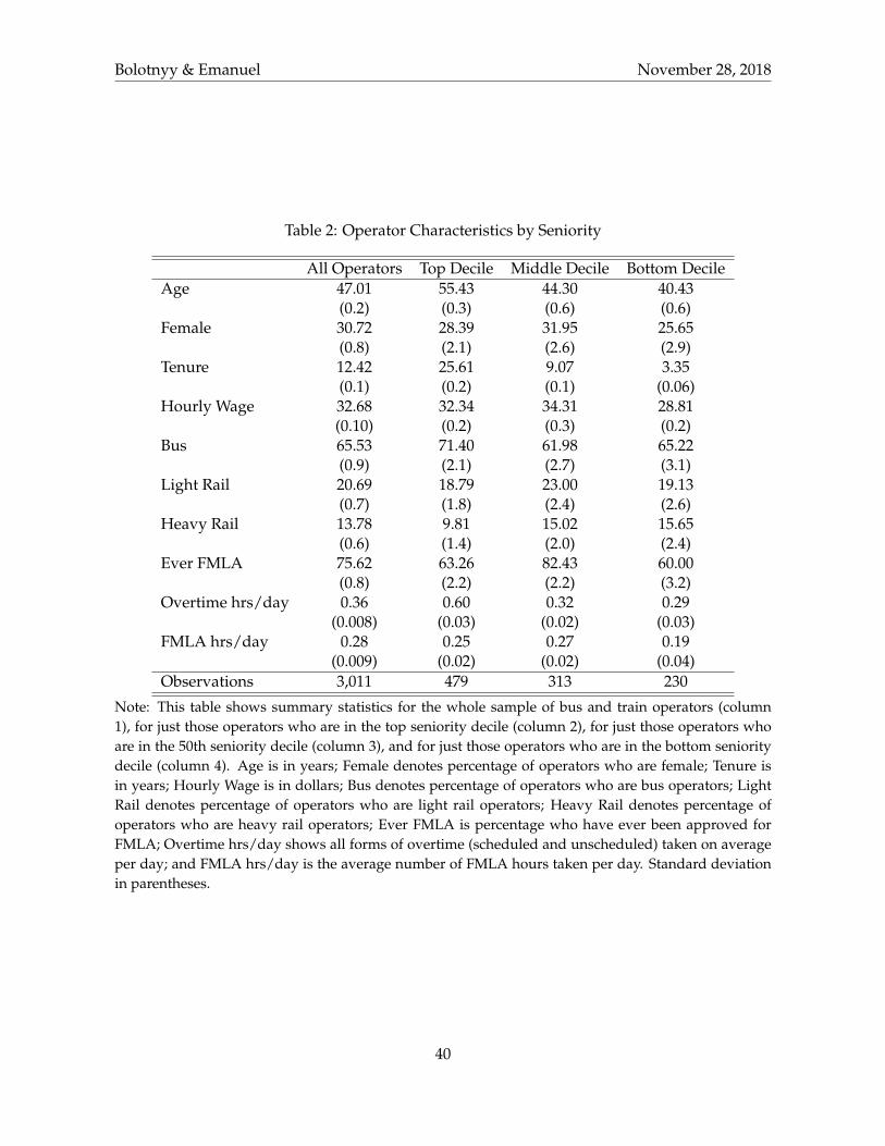
Bolotnyy & Emanuel November 28, 2018
Table 2: Operator Characteristics by Seniority
All Operators Top Decile Middle Decile Bottom DecileAge 47.01 55.43 44.30 40.43
(0.2) (0.3) (0.6) (0.6)Female 30.72 28.39 31.95 25.65
(0.8) (2.1) (2.6) (2.9)Tenure 12.42 25.61 9.07 3.35
(0.1) (0.2) (0.1) (0.06)Hourly Wage 32.68 32.34 34.31 28.81
(0.10) (0.2) (0.3) (0.2)Bus 65.53 71.40 61.98 65.22
(0.9) (2.1) (2.7) (3.1)Light Rail 20.69 18.79 23.00 19.13
(0.7) (1.8) (2.4) (2.6)Heavy Rail 13.78 9.81 15.02 15.65
(0.6) (1.4) (2.0) (2.4)Ever FMLA 75.62 63.26 82.43 60.00
(0.8) (2.2) (2.2) (3.2)Overtime hrs/day 0.36 0.60 0.32 0.29
(0.008) (0.03) (0.02) (0.03)FMLA hrs/day 0.28 0.25 0.27 0.19
(0.009) (0.02) (0.02) (0.04)Observations 3,011 479 313 230
Note: This table shows summary statistics for the whole sample of bus and train operators (column1), for just those operators who are in the top seniority decile (column 2), for just those operators whoare in the 50th seniority decile (column 3), and for just those operators who are in the bottom senioritydecile (column 4). Age is in years; Female denotes percentage of operators who are female; Tenure isin years; Hourly Wage is in dollars; Bus denotes percentage of operators who are bus operators; LightRail denotes percentage of operators who are light rail operators; Heavy Rail denotes percentage ofoperators who are heavy rail operators; Ever FMLA is percentage who have ever been approved forFMLA; Overtime hrs/day shows all forms of overtime (scheduled and unscheduled) taken on averageper day; and FMLA hrs/day is the average number of FMLA hours taken per day. Standard deviationin parentheses.
40

Bolotnyy & Emanuel November 28, 2018
Table 3: Probability of Accepting Overtime, Conditional on Being Offered
Any OT Any OT Weekend OT Working OTFemale -0.047*** -0.044*** -0.044*** -0.046***
(0.0003) (0.0003) (0.0006) (0.0004)
Constant 0.096*** 0.084*** 0.053*** 0.108***(0.0002) (0.0009) (0.0018) (0.0012)
Controls No Yes Yes YesMale Mean 0.096 0.106 0.109Adjusted R2 0.006 0.011 0.015 0.013Observations 3,747,826 3,747,089 995,462 2,246,614
Note: Outcomes are dummy variables that equal 1 if OT was accepted on any day (Any OT), on aweekend (Weekend OT), or on a working day (Working OT). Controls include age, tenure, senioritydecile, and garage fixed effects. Standard errors in parentheses. * = p<0.05, ** = p<0.01, *** = p<0.001.
41
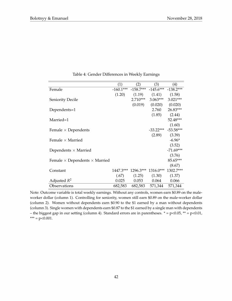
Bolotnyy & Emanuel November 28, 2018
Table 4: Gender Differences in Weekly Earnings
(1) (2) (3) (4)Female -160.1*** -158.7*** -145.6*** -138.2***
(1.20) (1.19) (1.41) (1.58)Seniority Decile 2.710*** 3.063*** 3.021***
(0.019) (0.020) (0.020)Dependents=1 2.760 26.83***
(1.85) (2.44)Married=1 52.48***
(1.60)Female × Dependents -33.22*** -53.58***
(2.89) (3.39)Female × Married -6.96*
(3.52)Dependents × Married -71.69***
(3.76)Female × Dependents × Married 85.65***
(8.67)Constant 1447.3*** 1296.3*** 1316.0*** 1302.7***
(.67) (1.25) (1.30) (1.37)Adjusted R2 0.025 0.053 0.064 0.066Observations 682,583 682,583 571,344 571,344
Note: Outcome variable is total weekly earnings. Without any controls, women earn $0.89 on the male-worker dollar (column 1). Controlling for seniority, women still earn $0.89 on the male-worker dollar(column 2). Women without dependents earn $0.90 to the $1 earned by a man without dependents(column 3). Single women with dependents earn $0.87 to the $1 earned by a single man with dependents– the biggest gap in our setting (column 4). Standard errors are in parentheses. * = p<0.05, ** = p<0.01,*** = p<0.001.
42

Bolotnyy & Emanuel November 28, 2018
Tabl
e5:
Sche
dule
dvs
.Uns
ched
uled
Ove
rtim
e
(1)
(2)
(3)
(4)
(5)
(6)
Sche
dO
TU
nsch
edO
TSc
hed
OT
Uns
ched
OT
Sche
dO
TU
nsch
edO
TFe
mal
e(Y
es=1
)-0
.107
***
-0.4
75**
*-0
.069
1***
-0.4
56**
*-0
.071
5***
-0.3
94**
*(0
.006
53)
(0.0
0901
)(0
.007
81)
(0.0
113)
(0.0
0877
)(0
.012
7)D
epen
dent
s(Y
es=1
)-0
.044
7***
-0.0
0034
4-0
.068
1***
0.12
3***
(0.0
0995
)(0
.014
4)(0
.013
1)(0
.018
9)Fe
mal
e×
Dep
ende
nts
-0.0
200
-0.0
470*
0.01
44-0
.204
***
(0.0
159)
(0.0
230)
(0.0
185)
(0.0
267)
Mar
ried
=10.
0316
***
0.21
5***
(0.0
0866
)(0
.012
5)Fe
mal
e×
Mar
ried
0.03
29-0
.211
***
(0.0
195)
(0.0
280)
Dep
ende
nts×
Mar
ried
0.04
30*
-0.3
47**
*(0
.020
4)(0
.029
4)Fe
mal
e×
Dep
ende
nts×
Mar
ried
-0.1
19*
0.76
4***
(0.0
475)
(0.0
687)
Con
stan
t-0
.044
6**
1.17
6***
-0.0
340
1.16
0***
-0.0
288
1.14
5***
(0.0
170)
(0.0
238)
(0.0
178)
(0.0
261)
(0.0
179)
(0.0
262)
Con
trol
sYe
sYe
sYe
sYe
sYe
sYe
sA
djus
ted
R2
0.13
30.
073
0.09
60.
060
0.09
60.
063
Obs
erva
tion
s12
9,31
814
1,41
411
0,44
612
0,35
711
0,44
612
0,35
7
Not
e:O
utco
me
vari
able
sar
e:1)
Sche
dO
T:lo
gho
urs
ofsc
hedu
led
over
tim
ew
orke
dpe
rmon
th,w
here
sche
dule
dov
erti
me
isse
lect
eda
quar
ter
(thr
eem
onth
s)in
adva
nce;
2)U
nsch
edO
T:lo
gho
urs
ofun
sche
dule
dov
erti
me
wor
ked
per
mon
th,w
here
unsc
hedu
led
over
tim
eis
offe
red
ada
yin
adva
nce
oron
the
sam
eda
yas
the
over
tim
esh
ift.
Con
trol
sin
clud
eag
e,te
nure
,sen
iori
tyde
cile
,and
gara
gefix
edef
fect
s.St
anda
rder
rors
inpa
rent
hese
s.*
=p<
0.05
,**
=p<
0.01
,***
=p<
0.00
1.
43

Bolotnyy & Emanuel November 28, 2018
Figure 1: The Gender Earnings Gap Across Seniority
Figure 1: Panel A shows that average monthly earnings (y axis) for bus and train operators in each senioritydecile (x axis). Across the seniority spectrum, women earn less than men. At lowest seniority, women make about$4,600/month while men earn about $5,200/month. At highest seniority, women make about $6,300/month, whilemen earn almost $7,000/month. Seniority is determined for full time operators based on which operator has thelongest tenure within his or her garage each quarter. Seniority determines the order in which routes, schedules,and holidays are picked, as well as who has first access to overtime opportunities. Panel B shows average monthlyearnings (y axis) for men and women without dependents for each seniority decile. Women without dependentsearn less than men without dependents across the seniority ladder.
44

Bolotnyy & Emanuel November 28, 2018
Figure 2: Accounting for the Gender Earnings Gap
Figure 2: We perform an accounting exercise to understand the gender earnings gap. We calculate scheduledearnings based on the hours each operator is scheduled to work at his/her regular wage. We then add in theovertime hours (scheduled and unscheduled) that the operator actually works at 1.5 times his/her regular wage.Total earnings are scheduled earnings plus overtime earnings, less the earnings forgone due to unpaid leave (FMLAand unexcused). The x axis shows seniority deciles, while the y axis shows monthly earnings in dollars. Each pointis the average for operators in a given seniority decile. Panel A plots the series for male operators, Panel B forfemale operators, Panel C for male operators with dependents, and Panel D for female operators with dependents.
45

Bolotnyy & Emanuel November 28, 2018
Figure 3: Differences in Pension-Eligible Earnings
Figure 3: Conditional on seniority, where men and women have the same choice sets of schedules and routes,women take work less pension-eligible hours than men. These pension eligible hours include regular work hoursand some forms of overtime. Built-in overtime, which takes workers slightly over an 8 hour work day due to theneed to, for example, bring a bus or train back to the garage and trippers, which are extra pieces of work on top of aregular schedule, count towards pension calculations. Annual pension payments are calculated as 2.46% times theaverage of the operator’s three highest paying years times years of service. The highest paying years are most likelygoing to be the last year’s of an operator’s career since his wage increases steadily with inflation over time andsince most of the built-in overtime and tripper overtime opportunities are made available first to the most senioroperators.
46

Bolotnyy & Emanuel November 28, 2018
Figure 4: Exogenous Arrival of Overtime Opportunities
Figure 4: This figure demonstrates how we are able to exploit the seniority structure of overtime offer rules toobtain exogenous variation in the availability of overtime. In this example, we have three operators ranked byseniority. For all but the most senior operator, the availability of overtime depends on whether those more seniorthan him accept or reject an overtime opportunity. Assuming, we think plausibly, that no individual operator canmeaningfully affect the decisions of those more senior than him, we can treat the arrival of an overtime opportunityas a Poisson process.
47

Bolotnyy & Emanuel November 28, 2018
Figure 5: Difference in Probability of Overtime Acceptance BetweenMen and Women
Figure 5: The arrival of overtime opportunities for any individual operator is a Poisson process, allowing us to usethe process by which overtime is offered to measure male and female probabilities of accepting overtime. Do obtainthe difference between male and female probabilities of accepting overtime, we regress a dummy for acceptingovertime conditional on being offered on a dummy variable for female and controls for age, tenure, seniority, andgarage fixed effects. We can see that, on average, men are about 3.8 to 5 percentage points more likely than womento accept an overtime opportunity, with some variation by day type.
48

Bolotnyy & Emanuel November 28, 2018
Figure 6: Distribution of Male and Female Probabilities of AcceptingOvertime, Conditional on Being Offered
Figure 6: We calculate the probability of accepting overtime conditional on being offered an opportunity for eachperson over our entire sample. This figure shows the distributions of these probabilities for men and women.There are more men than women who accepted overtime opportunities more than 50% of the time, while there areabout twice as many women as men who decline overtime opportunities all the time. The blue dashed vertical linemarks the male mean probability of accepting overtime. The orange dashed vertical line marks the female meanprobability of accepting overtime.
49

Bolotnyy & Emanuel November 28, 2018
Figure 7: Difference in Probability of Overtime Acceptance BetweenMen and Women, By Dependent Status
Figure 7: The arrival of overtime opportunities for any individual operator is a Poisson process, allowing us to usethe seniority system by which overtime is offered to measure male and female probabilities of accepting overtime.To obtain the difference between male and female probabilities of accepting overtime, we regress a dummy variablefor accepting overtime conditional on being offered on a dummy variable for female and controls for age, tenure,seniority, and garage fixed effects. We run separate regressions here for operators with and without dependents.Our results suggest that the presence of dependents plays a role in how men and women value time and how likelythey are to accept overtime opportunities. Men with dependents are more likely than women with dependents toaccept overtime and that gap is bigger than the gap between men and women who do not have dependents.
50

Bolotnyy & Emanuel November 28, 2018
Figure 8: Difference in Probability of Overtime Acceptance BetweenMen and Women, By Marital Status
Figure 8: The arrival of overtime opportunities for any individual operator is a Poisson process, allowing us to usethe seniority system by which overtime is offered to measure male and female probabilities of accepting overtime.To obtain the difference between male and female probabilities of accepting overtime, we regress a dummy variablefor accepting overtime conditional on being offered on a dummy variable for female and controls for age, tenure,seniority, and garage fixed effects. We run separate regressions here for operators who are and who are not married.Our results suggest that marital status plays a role in how men and women value time and how likely they are toaccept overtime opportunities. Married men are more likely than married women to accept overtime and that gapis bigger than the gap between men and women who are single.
51

Bolotnyy & Emanuel November 28, 2018
Figure 9: Difference in Probability of Overtime Acceptance BetweenSingle Men and Women, By Dependent Status
Figure 9: The arrival of overtime opportunities for any individual operator is a Poisson process, allowing us to usethe seniority system by which overtime is offered to measure male and female probabilities of accepting overtime.To obtain the difference between male and female probabilities of accepting overtime, we regress a dummy variablefor accepting overtime conditional on being offered on a dummy variable for female and controls for age, tenure,seniority, and garage fixed effects. We focus on single operators and run separate regressions for operators with andwithout dependents. Our results suggest that the presence of dependents for single operators plays an especiallybig role in how men and women value time and how likely they are to accept overtime opportunities. Single menwith dependents are considerably more likely than single women with dependents to accept overtime and that gapis bigger than the gap between single men and women who do not have dependents.
52

Bolotnyy & Emanuel November 28, 2018
Figure 10: Difference in Probability of Overtime Acceptance BetweenMarried Men and Women, By Dependent Status
Figure 10: The arrival of overtime opportunities for any individual operator is a Poisson process, allowing us to usethe seniority system by which overtime is offered to measure male and female probabilities of accepting overtime.To obtain the difference between male and female probabilities of accepting overtime, we regress a dummy variablefor accepting overtime conditional on being offered on a dummy variable for female and controls for age, tenure,seniority, and garage fixed effects. We focus on married operators and run separate regressions for operators withand without dependents. Our results suggest that the presence of dependents for married operators plays a rolein how men and women value time and how likely they are to accept overtime opportunities. Married men withdependents are only slightly more likely than married women with dependents to accept overtime. The gap inacceptance probability is high, though, between married men and women who do not have dependents, suggestingthat for them the division of household responsibilities and bread-winning is one that sees men taking on morework outside the home.
53

Bolotnyy & Emanuel November 28, 2018
Figure 11: Probability of Weekend Shift in Any Given Week
Figure 11: This binscatter displays the average probability for each seniority decile that an operator will have towork a weekend shift. The least senior operators, around the 10th percentile, are almost guaranteed to have to worka weekend shift. As seniority increases, the probability of having to work a weekend shift decreases, suggestingthat weekend shifts are undesirable. Conditional on seniority, which is the same as conditioning on the same choiceset of schedules and routes, women try to avoid scheduling weekend shifts more than men.
54

Bolotnyy & Emanuel November 28, 2018
Figure 12: Women Are Less Likely Than Men To Work Weekend Shifts
Figure 12: This charts shows, for each seniority decile, the differences in the average female probability of workinga weekend shift and the average male probability of working a weekend shift. Regressions to measure these differ-ences control for age, tenure, marital status, and quarter and garage fixed effects. The differences are negligible atlow seniority levels and grow with seniority. Women try to avoid scheduling weekend shifts more than men in astatistically significant way.
55
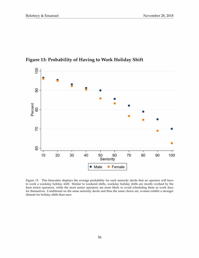
Bolotnyy & Emanuel November 28, 2018
Figure 13: Probability of Having to Work Holiday Shift
Figure 13: This binscatter displays the average probability for each seniority decile that an operator will haveto work a weekday holiday shift. Similar to weekend shifts, weekday holiday shifts are mostly worked by theleast senior operators, while the most senior operators are more likely to avoid scheduling them as work daysfor themselves. Conditional on the same seniority decile and thus the same choice set, women exhibit a strongerdistaste for holiday shifts than men.
56

Bolotnyy & Emanuel November 28, 2018
Figure 14: Probability of Split Shift on Any Given Day
Figure 14: This binscatter displays the average probability for each seniority decile that an operator will have towork a split shift on a given day. Working a split shift means not working 8 hours straight, but instead workinga few hours (usually during the morning rush hour), followed by a big break or split, and then the remaininghours (usually during the evening rush hour). The least senior male operators, around the 10th percentile, are verylikely to have to work a split shift. As seniority increases, the probability of having to work a split shift decreases,suggesting that split shifts are undesirable. Conditional on seniority, which is the same as conditioning on the samechoice set of schedules and routes, women try to avoid scheduling split shifts more than men. Only at high seniority,when they have the largest choice over the times of day during which the splits occur and their lengths, do womenchoose split shifts at similar rates to men.
57

Bolotnyy & Emanuel November 28, 2018
Figure 15: Accidents on Scheduled Bus Routes
Figure 15: For each bus route, we calculate the number of accidents (collisions with other vehicles, assaults on theoperator, passenger falls, etc.) experienced by male operators in 2014-2017. We use data for 2017Q4 on which routewas scheduled for which operator to calculate the number of men driving each route each quarter. Assuming thatthe number is roughly the same across all quarters of the year, we calculate the number of men driving each routeeach year. We divide the number of accidents by the number of male operators working each route each year andby 4 years to get the average number of accidents per male operator per year on each route. The series plotted hereshow, for each seniority decile, the average route scores for routes picked by women and men for 2017Q4.
58

Bolotnyy & Emanuel November 28, 2018
Figure 16: Difference Between Weekend Shift Weeks and Non-Weekend Shift Weeks
Figure 16: This chart shows how FMLA and overtime hours taken by men and women differ on weeks when theyare scheduled to work a weekend shift from those weeks when they are not scheduled to work a weekend shift. Werun person-week regressions of FMLA hours taken per week on a dummy variable for whether or not a weekendshift was scheduled in a particular week, as well as controls for age, tenure, seniority, and operator and month fixedeffects. We run these regressions separately for male and female operators. Point estimates for the coefficient on theweekend shift dummy and 95% confidence intervals are presented here. The chart shows that during weeks withweekend shifts, men take more unpaid FMLA hours off and work similarly more overtime, in essence substitutingpay at base wage for pay at the overtime rate of 1.5 X base wage. Women, on the other hand, take considerablymore unpaid FMLA hours of leave during weekend shift weeks, but only work a little bit more overtime. Thus,during weeks with weekend shifts, men earn more than during weeks without weekend shifts, while women earnless.
59

Bolotnyy & Emanuel November 28, 2018
Figure 17: Difference Between Holiday Shift Weeks and Non-HolidayShift Weeks
Figure 17: This chart shows how FMLA and unscheduled overtime hours taken by men and women differ onweeks when they are scheduled to work a holiday shift from those weeks when they are not scheduled to work aholiday shift. We run person-week regressions of FMLA hours taken per week on a dummy variable for whetheror not a holiday shift was scheduled in a particular week, as well as controls for age, tenure, seniority, and operatorand month fixed effects. We run these regressions separately for male and female operators. Point estimates forthe coefficient on the holiday shift dummy and 95% confidence intervals are presented here. The chart shows thatduring weeks with holiday shifts, men and women take take more unpaid FMLA hours off, with the increase largerfor women than for men. Men and women also work more overtime in weeks with holiday shifts, possibly becausemore overtime is available. The increase is bigger for men than for women. Unlike women, men more than makeup the unpaid hours with overtime hours.
60

Bolotnyy & Emanuel November 28, 2018
Figure 18: Difference Between Split Shift Days and Non-Split ShiftDays
Figure 18: This chart shows how FMLA and overtime hours taken by men and women differ on days when theyare scheduled to work a split shift from those days when they are not scheduled to work a split shift. We runperson-week regressions of FMLA hours taken per day on a dummy variable for whether or not a split shift wasscheduled in a particular day, as well as controls for age, tenure, seniority, and operator and month fixed effects.We run these regressions separately for male and female operators. Point estimates for the coefficient on the splitshift dummy and 95% confidence intervals are presented here. The chart shows that during days with split shifts,men take more unpaid FMLA hours off and work similarly more overtime, in essence substituting pay at base wagefor pay at the overtime rate of 1.5 X base wage. Women, on the other hand, take considerably more unpaid FMLAhours of leave during split shift days, but only work a little bit more overtime. Thus, during days with split shifts,men on average earn more than during days without split shifts, while women earn less.
61

Bolotnyy & Emanuel November 28, 2018
Figure 19: Number of FMLA Hours, Per Quarter
Figure 19: This chart shows how the average number of hours that operators take of FMLA per quarter changesthroughout our sample, from 2011 through 2017. The vertical dashed line at 2016Q1 represents the MBTA’s policychange on FMLA. In March of 2016, the MBTA hired UPMC Work Partners to be a third-party administrator incharge of making sure that FMLA certification was obtained and used properly. UPMC would now ensure thatdoctor’s notes certifying FMLA eligibility were legitimate and that, on a day-to-day basis, operators took FMLAleave in the way that the doctor deemed might be necessary. This policy change took the active FMLA certificationrate at the MBTA down from 45% to 27% of all operators. As the chart shows, the drop in FMLA usage was mostpronounced for female operators, but also present for male operators.
62

Bolotnyy & Emanuel November 28, 2018
Figure 20: FMLA Leave vs. Unexcused Leave, Before & After PolicyChange
Figure 20: Panel A shows the relationship between FMLA hours of leave taken in 2014 and the amount of unexcusedhours of leave taken in 2015. Panel B shows the relationship between FMLA hours taken in 2015 and the amountof unexcused hours of leave taken in 2017. Observations are at the person-year level. There is a close-to-constantrelationship between the two types of leave across years 2014 and 2015, for both men and women, and an upwardsloping relationship for both men and women across years 2015 and 2017.
63

Bolotnyy & Emanuel November 28, 2018
Figure 21: Discipline Severity and Unexcused Events
Figure 21: This chart shows the relationship, for men and women, between the average number of unexcusedevents and discipline severity. An unexcused event is an absence or a tardy without a legitimate excuse. Disciplineseverity ranges from a written warning (step 1) to a 3 day suspension without the ability to work overtime for thenext 45 calendar days (step 3) to a 70 day suspension and a recommendation for discharge (step 5).
64

Bolotnyy & Emanuel November 28, 2018
Figure 22: Hours of Unexcused Leave, By Quarter and Gender
Figure 22: Panel A shows, from the first quarter of 2011 to the last quarter of 2017, the average number of hoursof unexcused leave taken by operators of each gender. The left-most dashed vertical line denotes the introductionof the FMLA policy (March 2016) and the right-most dashed vertical line denotes the introduction of the overtimepolicy (July 2017). Panel B follows the same structure, but plots the series for men and women without dependents.Panel C plots the series for men and women with dependents.
65

Bolotnyy & Emanuel November 28, 2018
Figure 23: Number of Overtime Hours, Per Quarter
Figure 23: This chart shows how the average number of hours that operators take of overtime per quarter changesthroughout our sample, from 2011 through 2017. The vertical dashed line at 2016Q1 represents the MBTA’s policychange on FMLA. In March of 2016, the MBTA hired UPMC Work Partners to be a third-party administrator incharge of making sure that FMLA certification was obtained and used properly. UPMC would now ensure thatdoctor’s notes certifying FMLA eligibility were legitimate and that, on a day-to-day basis, operators took FMLAleave in the way that the doctor deemed might be necessary. This policy change took the active FMLA certificationrate at the MBTA down from 45% to 27% of all operators. The dashed line at 2017Q3 shows the timing of theintroduction of the MBTA’s new policy on overtime. Overtime went from being defined as any time in excess of 8hours worked in a day to any time in excess of 40 hours worked in a week. The result was a drop in the averagenumber of overtime hours worked by male operators from 40 hours per quarter to about 10 hours per quarter.Female hours dropped as well, but my a considerably smaller amount.
66

Bolotnyy & Emanuel November 28, 2018
Figure 24: Of Those Who Took FMLA in a Given Week, What PercentAlso Took Overtime That Week?
Figure 24: This chart shows the share of operators who took FMLA in a given week who also took overtime thatweek, by gender. Men are more likely than women to take both overtime and FMLA in a week where they aretaking FMLA leave both in 2011-2015 and in 2016-2017, after the FMLA and overtime policy changes. However, theshare of men and women doing both overtime and FMLA, conditional on taking FMLA, falls in 2016-2017 and thegap between men and women shrinks.
67

Bolotnyy & Emanuel November 28, 2018
Figure 25: Weeks with Weekend Shifts vs. No Weekend Shifts, Beforevs. After Policy Changes
Figure 25: This chart shows how FMLA and overtime hours taken by men and women differ on weeks when theyare scheduled to work a weekend shift from those weeks when they are not scheduled to work a weekend shift.The greyed-out points use data for 2011-2015 to measure the intensity of these differences prior to the 2016-2017policy changes that made it harder to take FMLA time off and to work overtime. The observations in full colorshow the differences in 2016-2017, when the policy changes were taking place. We run person-week regressions ofFMLA hours taken per week on a dummy variable for whether or not a weekend shift was scheduled in a particularweek, as well as controls for age, tenure, seniority, and operator and month fixed effects. We run these regressionsseparately for male and female operators. The chart shows that during weeks with weekend shifts, men take moreunpaid FMLA hours off and work similarly more overtime, in essence substituting pay at base wage for pay at theovertime rate of 1.5 X base wage. Women, on the other hand, take considerably more unpaid FMLA hours of leaveduring weekend shift weeks, but only work a little bit more overtime. Thus, during weeks with weekend shifts,men earn more than during weeks without weekend shifts, while women earn less. These patterns, however, aremuch stronger in the 2011-2015 period, before the policy changes took place in 2016-2017.
68

Bolotnyy & Emanuel November 28, 2018
Figure 26: Lost Trips and Leave-Taking
Figure 26: Panel A shows the relationship between the number of lost trips in a particular garage on a particularday as a result of operator absence (y axis) and the total number of FMLA hours of leave taken by operators in thatsame garage on that same day (x axis). The relationship is residualized (we are controlling for week and garagefixed effects), resulting in some of the visualized points being in negative FMLA hour territory. Panel B showsthe relationship between the number of lost trips as a result of operator absence (y axis) and the total number ofunexcused hours of leave taken by operators in that same garage on that same day (x axis). The relationship is alsoresidualized. The slopes of the unconditional relationships are similar to the ones reported here. Standard errorsare in parentheses. Lost trips data are available for 2014-2017, so the chart shows relationships only for those years.
69

Bolotnyy & Emanuel November 28, 2018
APPENDIX
Service Map, Massachusetts Bay Transportation Authority
Figure A.1: A 2017 map of MBTA bus and train routes that service the Boston metropolitan area. Our data coverthe bus and train operators that service these routes.
70

Bolotnyy & Emanuel November 28, 2018
Job Description, Bus Operator
Figure A.2: A job posting for the 2017 bus operator lottery.
71
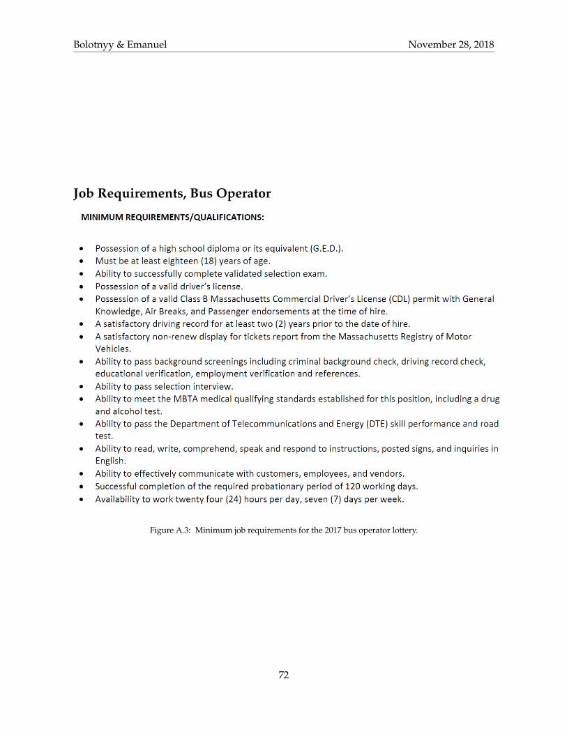
Bolotnyy & Emanuel November 28, 2018
Job Requirements, Bus Operator
Figure A.3: Minimum job requirements for the 2017 bus operator lottery.
72

Bolotnyy & Emanuel November 28, 2018
Job Description, Heavy Rail Operator
Figure A.4: A job posting for the 2017 heavy rail operator lottery.
73

Bolotnyy & Emanuel November 28, 2018
Job Requirements, Heavy Rail Operator
Figure A.5: Minimum job requirements for the 2017 heavy rail operator lottery.
74

Bolotnyy & Emanuel November 28, 2018
Share of Female Operators and Share of Operators Working Week-ends, By Garage
Figure A.6: This chart shows, for each garage, the share of operators working a weekend shift in any given week. Italso shows the share of female operators in each garage in any given week. The two dashed vertical lines separatethe bus garages from the light rail garage (Green Line) and the light rail garage from the heavy rail garages. Thereare slightly more female operators in the rail garages, while the share of operators working a weekend shift issimilar across garages.
75

Bolotnyy & Emanuel November 28, 2018
Example of a Quarterly Pick Sheet
Figure A.7: This is an example of a sheet that would be used during a quarterly process called "The Pick" duringwhich operators select the routes and times that they will work for the following quarter. This sheet applies toSaturday routes coming out of the Bennett garage in the Fall of 2016. Each row denotes a day of work.
76

Bolotnyy & Emanuel November 28, 2018
Share of Women Across Seniority Deciles
Figure A.8: Women make up a fairly consistent share of workers in each seniority level.
77

Bolotnyy & Emanuel November 28, 2018
Share of Female Operators, By Tenure
Figure A.9: Women make up a fairly consistent share of workers across tenure (in years of service) at the MBTA.
78

Bolotnyy & Emanuel November 28, 2018
Operator Age Across Seniority
Figure A.10: This chart shows the relationship between operator age and seniority. The least senior operators areon average about 40 years old, while the most senior operators are about 55 years old. The female operators are onaverage slightly younger than the male operators, across the seniority spectrum.
79

Bolotnyy & Emanuel November 28, 2018
CDF of Tenure at Termination
Figure A.11: This chart shows the cumulative distribution function (CDF) of operator tenure upon exiting theMBTA. The vast majority of these exits are voluntary. Discharge can occur for egregious misbehavior or frequentunexcused absenteeism. About 1% of the operators were discharged in 2016-2017 as a result of a new disciplinepolicy that made absenteeism a just cause of suspensions and recommendations for discharge. The data presentedhere show the CDF for 2011-2017 and include voluntary exits and discharges based on the new discipline policy.
80

Bolotnyy & Emanuel November 28, 2018
Share of Married Operators By Seniority
Figure A.12: This chart shows the share of men and women in each seniority decile that are married. We havesome attrition of single operators for men and women, with the most senior male and female operators lookingvery similar in terms of marital status.
81

Bolotnyy & Emanuel November 28, 2018
Base Wage by Seniority
Figure A.13: This chart shows the average base wage for each seniority decile. Operator wages rise until year 4 onthe job and then increase modestly with inflation for every year thereafter. Starting wages and wage increases candiffer based on an operator’s start date, due to changes in the collective bargaining agreement that gets renegotiatedevery 4 years.
82

Bolotnyy & Emanuel November 28, 2018
Base Wage by Tenure
Figure A.14: This chart shows the average base wage for each year of tenure. Operator wages rise until year 4 onthe job and then increase modestly with inflation for every year thereafter. Starting wages and wage increases candiffer based on an operator’s start date, due to changes in the collective bargaining agreement that gets renegotiatedevery 4 years.
83

Bolotnyy & Emanuel November 28, 2018
Probability of Taking FMLA, By Day and Gender
Figure A.15: This chart shows male and female probabilities of taking FMLA leave by day of week. The chartmakes clear that women take more FMLA than men and that certain days are more likely to see FMLA usage thanothers. Saturday, Friday, and Sunday, in that order, are the likeliest of all days of the week to see an operator takeunpaid time off, especially women. This variation suggests that FMLA is being used for something other than justmedically-necessary time off.
84
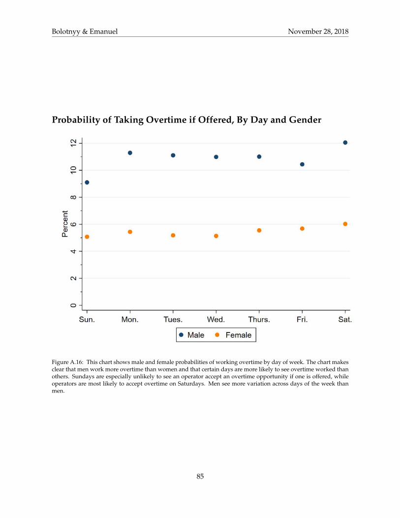
Bolotnyy & Emanuel November 28, 2018
Probability of Taking Overtime if Offered, By Day and Gender
Figure A.16: This chart shows male and female probabilities of working overtime by day of week. The chart makesclear that men work more overtime than women and that certain days are more likely to see overtime worked thanothers. Sundays are especially unlikely to see an operator accept an overtime opportunity if one is offered, whileoperators are most likely to accept overtime on Saturdays. Men see more variation across days of the week thanmen.
85
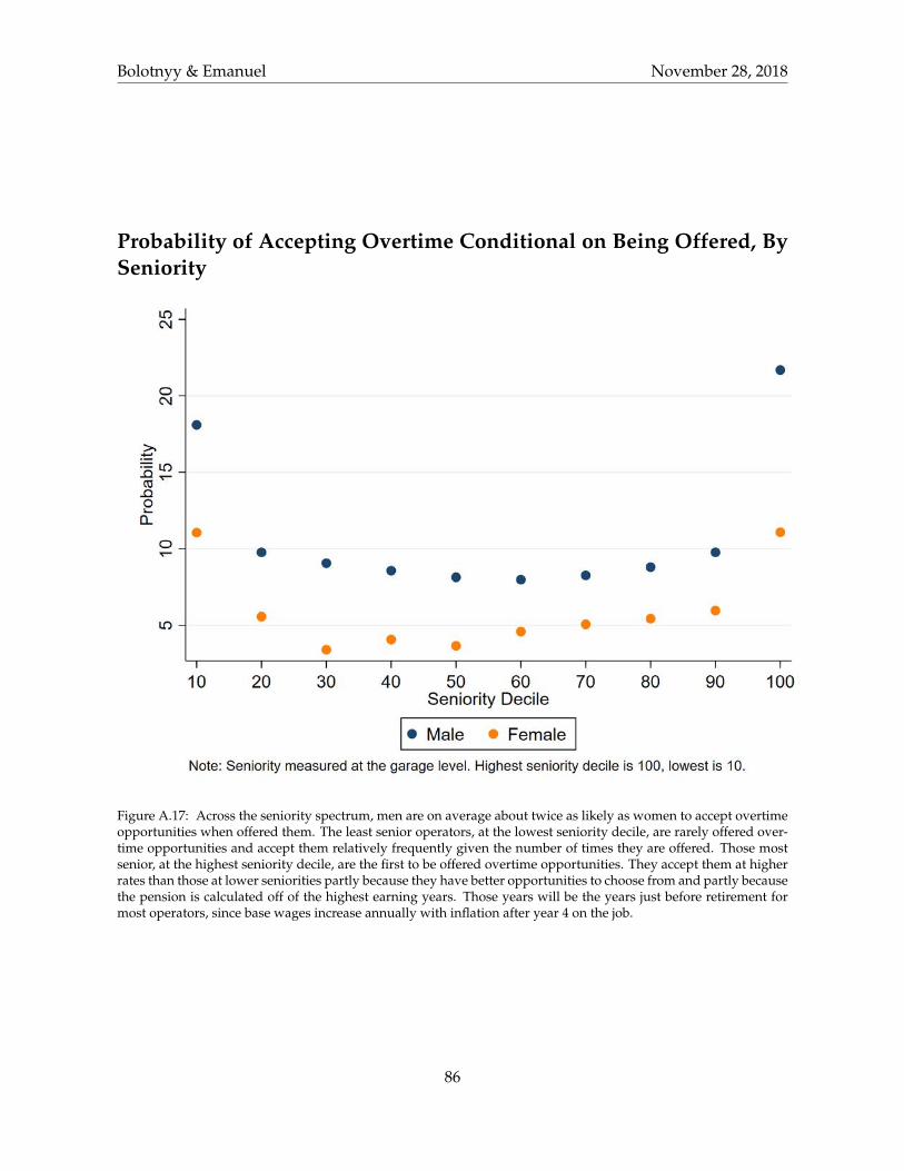
Bolotnyy & Emanuel November 28, 2018
Probability of Accepting Overtime Conditional on Being Offered, BySeniority
Figure A.17: Across the seniority spectrum, men are on average about twice as likely as women to accept overtimeopportunities when offered them. The least senior operators, at the lowest seniority decile, are rarely offered over-time opportunities and accept them relatively frequently given the number of times they are offered. Those mostsenior, at the highest seniority decile, are the first to be offered overtime opportunities. They accept them at higherrates than those at lower seniorities partly because they have better opportunities to choose from and partly becausethe pension is calculated off of the highest earning years. Those years will be the years just before retirement formost operators, since base wages increase annually with inflation after year 4 on the job.
86