Wildfires and Respiratory Illness: Linking Fire Events and Attributes to Health Outcomes

Klaus Moeltner Department of Agricultural and Applied Economics, Virginia Tech

moeltner@vt.edu

Man-Keun Kim Department of Applied Economics, Utah State University

mk.kim@usu.edu

Wei Yang School of Community Health Sciences, University of Nevada, Reno

weiyang@unr.edu

Erqian Zhu China Center for International Economic Exchange

erqian.zhu@gmail.com

Selected Paper prepared for presentation at the Agricultural & Applied Economics Association's 2011 AAEA & NAREA Joint Annual Meetings, Pittsburgh, Pennsylvania, July 24-26, 2011

Draft May 2, 20011

Preliminary and incomplete – please do not cite

Wildfires and Respiratory Illness: Linking Fire Eventsand Attributes to Health Outcomes

K. Moeltnera,∗, M.-K. Kimb, W. Yangc, E. Zhud

aDepartment of Agricultural and Applied Economics, Virginia TechbDepartment of Applied Economics, Utah State University

cSchool of Community Health Sciences, University of Nevada, RenodChina Center for International Economic Exchange

Abstract

Existing studies on the economic impact of wildfire smoke have focusedeither on single fire events or entire fire seasons without distinguishing be-tween individual occurrences. Neither approach allows for an examinationof the marginal effects of fire attributes, such as distance and fuel type, onhealth impacts and costs. Yet, improved knowledge of these marginal effectscan provide important guidance for efficient wildfire management strategies.This study aims to bridge this gap using detailed information on 35 large-scale wildfires in the California and Nevada Sierras that have sent smokeplumes to the Reno / Sparks area of Northern Nevada over a three-yearperiod. We relate the daily acreage burned by these fires to daily data onlocal hospital admissions for acute respiratory syndrome. Using informationon treatment expenses, we compute the per-acre cost of wildfires of differentattributes with respect to respiratory admissions. We find that while nearbyfires are four-five times more damaging than remote fires, hospital admis-sions can be causally linked to fires as far as 200-250 miles form the impactarea. Our results highlight the economic benefits of fire suppression, andthe importance of inter-regional agency collaboration in the management offorest fires.

Keywords: Wildfires, air quality, respiratory illness, distributed lagmodels, count data models

∗Corresponding author, mobile phone: (775)560-3288Email addresses: moeltner@vt.edu (K. Moeltner), mk.kim@usu.edu (M.-K. Kim),

weiyang@unr.edu (W. Yang), erqian.zhu@gmail.com (E. Zhu)

Draft - Preliminary and Incomplete May 2, 2011

1. Introduction

Optimal wildfire management policy requires information of the healtheffects and related economic costs caused by wildfire events. Kochi et al.(2010) synthesize existing studies that have examined the nexus of wildfires,air quality, and illness and conclude that there is still much to be learnedabout the causal impact of wildfires on health outcomes. Specifically, mostexisting contributions either consider a single fire event (Adamowicz et al.,2004; Viswanathan et al., 2006) or air quality changes over an entire fire sea-son without controlling for individual burn events (Johnston et al., 2002a,b;Tham et al., 2009). This preempts a closer investigation of the marginaleffects of even the most basic fire attributes, such as size, distance, and fuelload.

While there is a general notion that wildfire smoke can travel far beforereaching population centers, the question of how health impacts change overfire distance remains unadressed. Similarly, existing studies considering aspecific fire event have focused on the total health impact of the fire withina given time period, but not yet provided insights into the marginal effectper acre burned. Furthermore, given existing fuel models (Clinton et al.,2003) one can hypothesize that the latter will depend on the vegetationtype consumed by a given fire.

Knowledge of these marginal effects can provide important guidance forwildfire management. For example, as noted in Kochi et al. (2010) andKochi et al. (2011), averted health costs ought to be considered as one ofthe benefits of preemptive fuel reduction. Naturally, this requires knowl-edge on the marginal health cost per acre burned for areas that differ in fuelmanagement or composition. By the same token, the benefits of wildfiresuppression in remote areas will be under-estimated if no health cost avoid-ance value is assigned to such efforts, but smoke can nonetheless impact faraway population zones.

This study aims at providing first estimates of wildfire-generated airpollution on health costs, differentiated along several dimensions of fire at-tributes. This requires detailed data on daily fire progression and health out-comes. To our knowledge such data have not yet been collected or combinedin previous research. We benefit from what could be described as an ongoingnatural experiment: The urban area of Reno / Sparks in Northern Nevadatraditionally experiences smoke from numerous wildfire events every season.This is due to the typically dry conditions in the Sierra Nevada mountainrange and foothills that border this area to the west, and the prevailingand persistent north-western to south-western wind patterns. Furthermore,

2

some of these fires are as remote as 200 - 300 miles from the impact area,while others burn at the urban fringe. In addition, fires at any distance varyin fuel composition. They can occur in grassland, the sage/ juniper inter-face, or in large stands of mature timber. Thus, observing these fire eventsover several seasons provides the necessary variability in distance and fuelload to identify corresponding marginal effects.

At the same time, Nevada State law requires all hospitals to report dataon inpatient admissions to research centers at State universities. This infor-mation allows us to track daily hospital admissions for illnesses traditionallyrelated to severe air pollution over the same time period as the wildfire oc-currences. We then take a Cost-of-Illness (COI) approach relating fire eventsand attributes to treatment costs (Kochi et al., 2010).

The following section provides details on the different components ofour data set. Section III describes the econometric framework. Section IVdiscusses estimation results, and Section V concludes.

2. Data

2.1. Wildfire data

The time frame for our analysis ranges from March 3, 2005 to December30, 2008, for a total of 1399 days. This is based on the availability of dailydata on both air quality and and patient admissions. During this periodthe Reno / Sparks area experienced wind blowing from the northwest, west,and southwest for 67 percent of the time. Moreover, these wind directionsgoverned the area for 80 percent of all days during the fire season monthsof May through September. On a typical summer day, winds start with anorth-western direction in the morning, and then gradually rotate westwardand stabilize at a south-western direction by mid-afternoon. Thus, we con-sider all separate wildfires that burned during this time period and occurredanywhere from the north-west to the west and south-west of the impactarea. We allow for a distance radius of 500 miles and impose a minimumsize threshold of 300 acres, thus focusing on larger wildfires.1

The spatial distribution of the resulting 35 separate fire events is depictedin Figure 1. Table 1 captures fire details, i.e. total acres burned (in units of1000), start and end date, total duration in days, and distance from the Reno/ Sparks area. Overall, these fires consumed over 1.2 million acres over the

1Holmes et al. (2008) estimate that fires exceeding 500 acres account for 94 percent ofall acres burned in the Southern Sierra Nevada between 1910 and 2003.

3

research period. They range from a size of under 500 acres (”Vista Fire”) toover 190,000 acres (”Klamath Theater Fire”), for an average of 35,000 acres.Some of them were extinguished within a few days, while others burned formany weeks. The mean duration is close to 22 days, yielding a total of 767fire-days for our research period. Accounting for overlapping events, thistranslates into 296 separate days, or 21 percent of all research days, with atleast one active fire upwind of the impact area. As shown in the last columnof the table these fires occurred within a wide radius of Reno / Sparks, fromthe city limits to a distance of over 350 miles. The average distance is 148miles.

Reno / Sparks

NVCA

Figure 1: Location of wildfires and impact area

Wildfire information was obtained from the Western Great Basin Coor-dination Center (WGBCC) in Reno, Nevada, and the U.S. Forest Service’sIncident Management Situation (SIT) reports for the affected areas, avail-able online (National Fire and Aviation Management, 2011). Informationon the daily acres burned was provided by a GIS specialist at the U.S. ForestServices Pacific Southwest Research Station in Albany, California. We aug-ment and refine this Forest Service data with data from the daily fire trackingweb site of the Western Institute for Study of the Environment (W.I.S.E.), a

4

non-profit educational and research facility with headquarters in Corvallis,Oregon. This agency routinely collects daily fire information for the Westand Northwest based on official media reports and updates provided by var-ious federal and State agencies. It then posts the entire daily history for agiven fire on its fire tracking web site (Western Institute for Study of the En-vironment, 2011). For burn days for which information on daily fire growthwas not available (approximately 20-30% of fire-days) we estimate the con-sumed area via interpolation using the nearest known data points.

The entire time series of acres consumed by all relevant fires on a givencalendar day is shown in the top panel of Figure 2. As is evident from thefigure, the total number of daily acres burned ranges from a few hundred toover 40,000. There also appears to be a pattern of increasingly severe fireseasons over time, with the summer of 2008 marking the worst fire seasonin California since record keeping started in the 1970. We will relate thispanel to the time series on patient admissions and air pollution below.

date

valu

e

0

10000

20000

30000

40000

0

5

10

15

20

20

40

60

80

100

120

140

Mar−05 Sep−05 Mar−06 Sep−06 Mar−07 Sep−07 Mar−08 Sep−08 Mar−09

acrestotalpatients

pm25

Figure 2: Daily time series of pm2.5 (µg/m3), patient admissions, and acres burned

On a given fire-event day in our series an average of 2.34 fires burnedconcurrently, with a maximum of 11 (June 29-30, 2008). Naturally, this pre-empts a clear identification of the exact source of a unit of PM2.5 that reachesthe impact area on or near those days. We thus settle for a distinction oftotal daily acres burned by the following distance zones: (I) 0-50 miles, (II)

5

Table 1: Large Wildfires upwind of Reno / Sparks, 2005-2008

name State acres start end days distance

China Lake CA 5.3 7/19/2005 7/24/2005 5 123Comb Complex CA 8.675 7/22/2005 10/15/2005 85 96

Crag CA 1.2 7/24/2005 7/29/2005 5 85Empire NV 3 6/25/2006 6/28/2006 3 95Squaw NV 2.095 6/25/2006 6/26/2006 1 100

Bootlegger NV 6.669 7/6/2006 8/13/2006 38 40Jackass CA 6.255 7/17/2006 7/21/2006 4 80Verdi NV 5.661 8/11/2006 8/13/2006 2 5

August NV 0.641 9/2/2006 9/2/2006 0 261Day CA 162.702 9/4/2006 10/2/2006 28 358

Ralston CA 8.423 9/5/2006 9/17/2006 12 214Mustang CA 0.572 5/18/2007 5/19/2007 1 10

Bolli CA 0.732 5/22/2007 5/27/2007 5 292Honey NV 0.688 5/22/2007 5/23/2007 1 267Angora CA 3.1 6/24/2007 7/2/2007 8 60

Antelope Complex CA 136.777 7/5/2007 7/13/2007 8 101Balls Canyon CA 0.9 7/10/2007 7/13/2007 3 16

Hawken NV 2.708 7/16/2007 7/23/2007 7 0Sand Pass NV 6.999 7/17/2007 7/19/2007 2 50

Tar CA 5.642 8/10/2007 8/16/2007 6 33Vista CA 0.471 8/22/2007 8/27/2007 5 78North CA 2.2 9/2/2007 9/8/2007 6 103

East Lake NV 0.962 4/29/2008 4/30/2008 1 15Lime Complex CA 99.586 6/20/2008 8/15/2008 56 346

Klamath Theater CA 192.038 6/21/2008 9/30/2008 101 247Iron & Alps Complex CA 105.606 6/21/2008 9/1/2008 72 196Yolla Bolly Complex CA 89.663 6/21/2008 8/19/2008 59 311

Shu Lightning Complex CA 86.5 6/21/2008 7/25/2008 34 326BTU Lightning Complex CA 59.44 6/21/2008 7/29/2008 38 109

Canyon Complex CA 38.509 6/21/2008 8/14/2008 54 260American River Complex CA 20.541 6/21/2008 8/1/2008 41 221

Basin Complex CA 147.114 6/21/2008 7/27/2008 36 241Yuba River Complex CA 4.254 6/21/2008 7/15/2008 24 70

Corral CA 12.434 6/23/2008 7/7/2008 14 325Gooseberry NV 3.042 7/29/2008 7/31/2008 2 49.5

51-100 miles, (III) 101-250 miles, and (IV) > 250 miles. This yields anapproximately even distribution of fire incidents per zone. However, moredistant fires tend to be substantially larger than fires that occurred near theurban interface. Specifically, the average fire size, in total acres consumed,lies at close to 4,000 acres for distance zones I and II, and, respectively, at

6

75,000 and 55,000 for zones III and IV. This is as expected, as remote firesin the heart of the Sierras are generally more difficult to combat and thushave more time to grow in size.

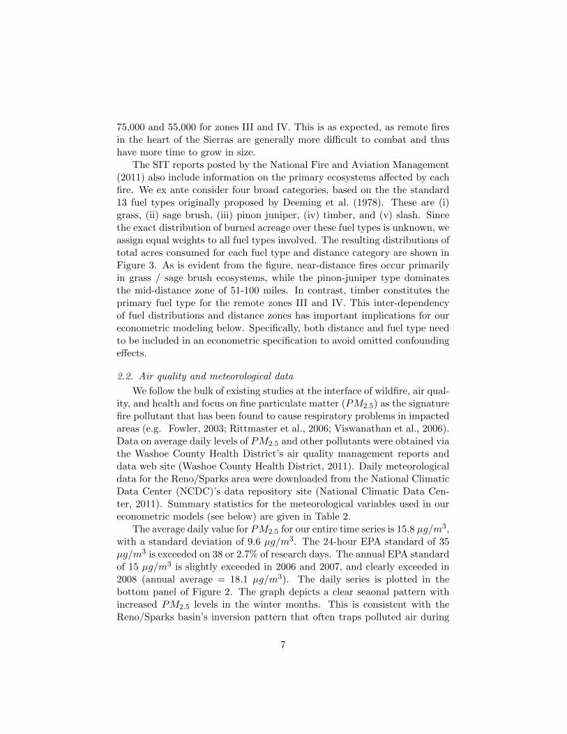
The SIT reports posted by the National Fire and Aviation Management(2011) also include information on the primary ecosystems affected by eachfire. We ex ante consider four broad categories, based on the the standard13 fuel types originally proposed by Deeming et al. (1978). These are (i)grass, (ii) sage brush, (iii) pinon juniper, (iv) timber, and (v) slash. Sincethe exact distribution of burned acreage over these fuel types is unknown, weassign equal weights to all fuel types involved. The resulting distributions oftotal acres consumed for each fuel type and distance category are shown inFigure 3. As is evident from the figure, near-distance fires occur primarilyin grass / sage brush ecosystems, while the pinon-juniper type dominatesthe mid-distance zone of 51-100 miles. In contrast, timber constitutes theprimary fuel type for the remote zones III and IV. This inter-dependencyof fuel distributions and distance zones has important implications for oureconometric modeling below. Specifically, both distance and fuel type needto be included in an econometric specification to avoid omitted confoundingeffects.

2.2. Air quality and meteorological data

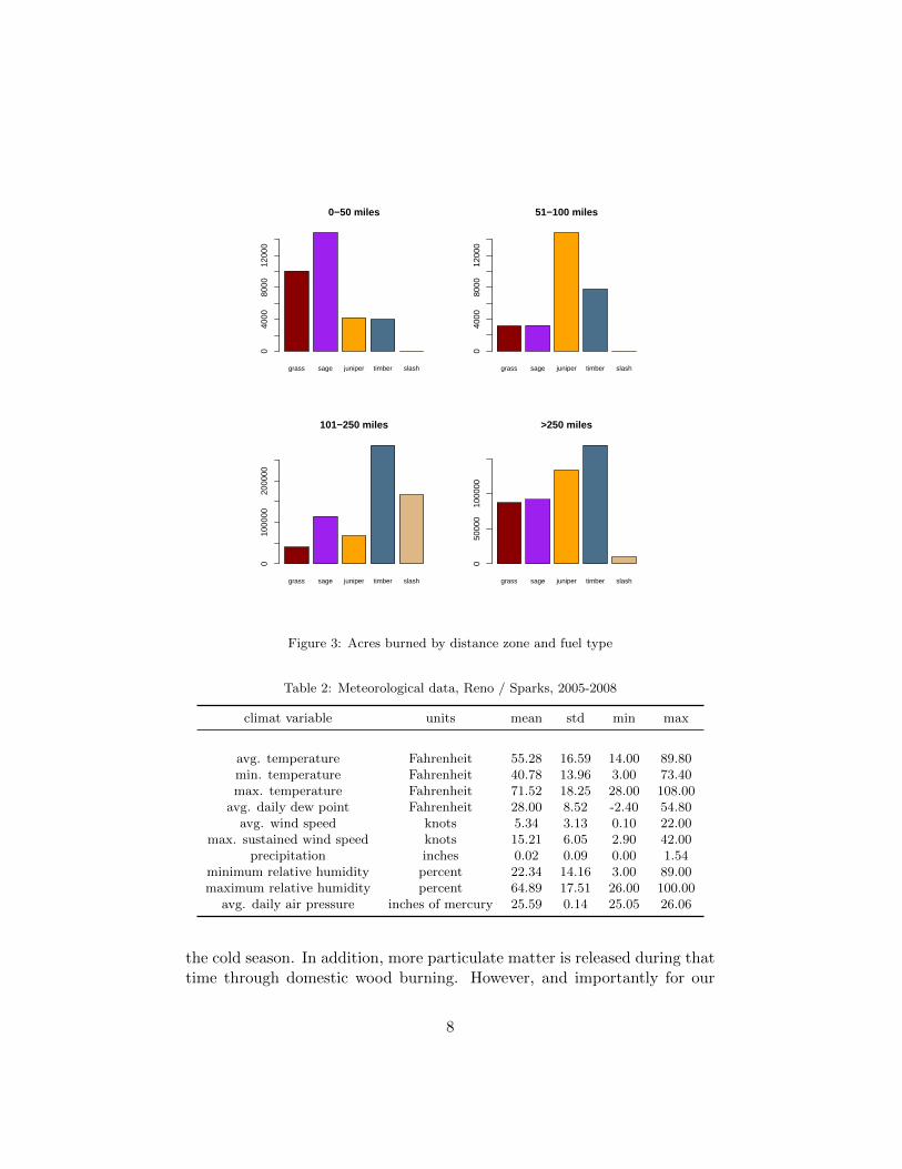
We follow the bulk of existing studies at the interface of wildfire, air qual-ity, and health and focus on fine particulate matter (PM2.5) as the signaturefire pollutant that has been found to cause respiratory problems in impactedareas (e.g. Fowler, 2003; Rittmaster et al., 2006; Viswanathan et al., 2006).Data on average daily levels of PM2.5 and other pollutants were obtained viathe Washoe County Health District’s air quality management reports anddata web site (Washoe County Health District, 2011). Daily meteorologicaldata for the Reno/Sparks area were downloaded from the National ClimaticData Center (NCDC)’s data repository site (National Climatic Data Cen-ter, 2011). Summary statistics for the meteorological variables used in oureconometric models (see below) are given in Table 2.

The average daily value for PM2.5 for our entire time series is 15.8 µg/m3,with a standard deviation of 9.6 µg/m3. The 24-hour EPA standard of 35µg/m3 is exceeded on 38 or 2.7% of research days. The annual EPA standardof 15 µg/m3 is slightly exceeded in 2006 and 2007, and clearly exceeded in2008 (annual average = 18.1 µg/m3). The daily series is plotted in thebottom panel of Figure 2. The graph depicts a clear seaonal pattern withincreased PM2.5 levels in the winter months. This is consistent with theReno/Sparks basin’s inversion pattern that often traps polluted air during

7

grass sage juniper timber slash

0−50 miles

040

0080

0012

000

grass sage juniper timber slash

51−100 miles

040

0080

0012

000

grass sage juniper timber slash

101−250 miles

010

0000

2000

00

grass sage juniper timber slash

>250 miles

050

000

1000

00

Figure 3: Acres burned by distance zone and fuel type

Table 2: Meteorological data, Reno / Sparks, 2005-2008

climat variable units mean std min max

avg. temperature Fahrenheit 55.28 16.59 14.00 89.80min. temperature Fahrenheit 40.78 13.96 3.00 73.40max. temperature Fahrenheit 71.52 18.25 28.00 108.00

avg. daily dew point Fahrenheit 28.00 8.52 -2.40 54.80avg. wind speed knots 5.34 3.13 0.10 22.00

max. sustained wind speed knots 15.21 6.05 2.90 42.00precipitation inches 0.02 0.09 0.00 1.54

minimum relative humidity percent 22.34 14.16 3.00 89.00maximum relative humidity percent 64.89 17.51 26.00 100.00

avg. daily air pressure inches of mercury 25.59 0.14 25.05 26.06

the cold season. In addition, more particulate matter is released during thattime through domestic wood burning. However, and importantly for our

8

research, the graph also shows a clear temporal correspondence of elevatedPM2.5 levels and daily acres burned, as can be gleaned from a comparisonof the top and bottom panels of Figure 2. This correlation is especiallyapparent during the ”record” 2008 fire season, with PM2.5 levels reachingpeaks of 140µg/m3 and higher.

2.3. Hospital data

Patient admissions data were provided by The Center for Health Infor-mation Analysis (CHIA) at the University of Nevada, Las Vegas, and theNevada Center for Health Statistics and Informatics at the University ofNevada, Reno. Under State law, these Centers collect and maintain billingrecords from Nevada hospital and ambulatory surgical centers. Among otherinformation, these medical outfits are required to submit daily inpatient datato these Centers on a regular basis. For this analysis we consider all res-piratory disease cases as captured by International Disease Codes (IDCs)460.0-486.99, and 488.0-519.99, except for influenza (IDC 487.00-487.99).The Nevada Center for Health Statistics and Informatics also made avail-able summary statistics of treatment length and costs for our targeted timeperiod and illness codes.

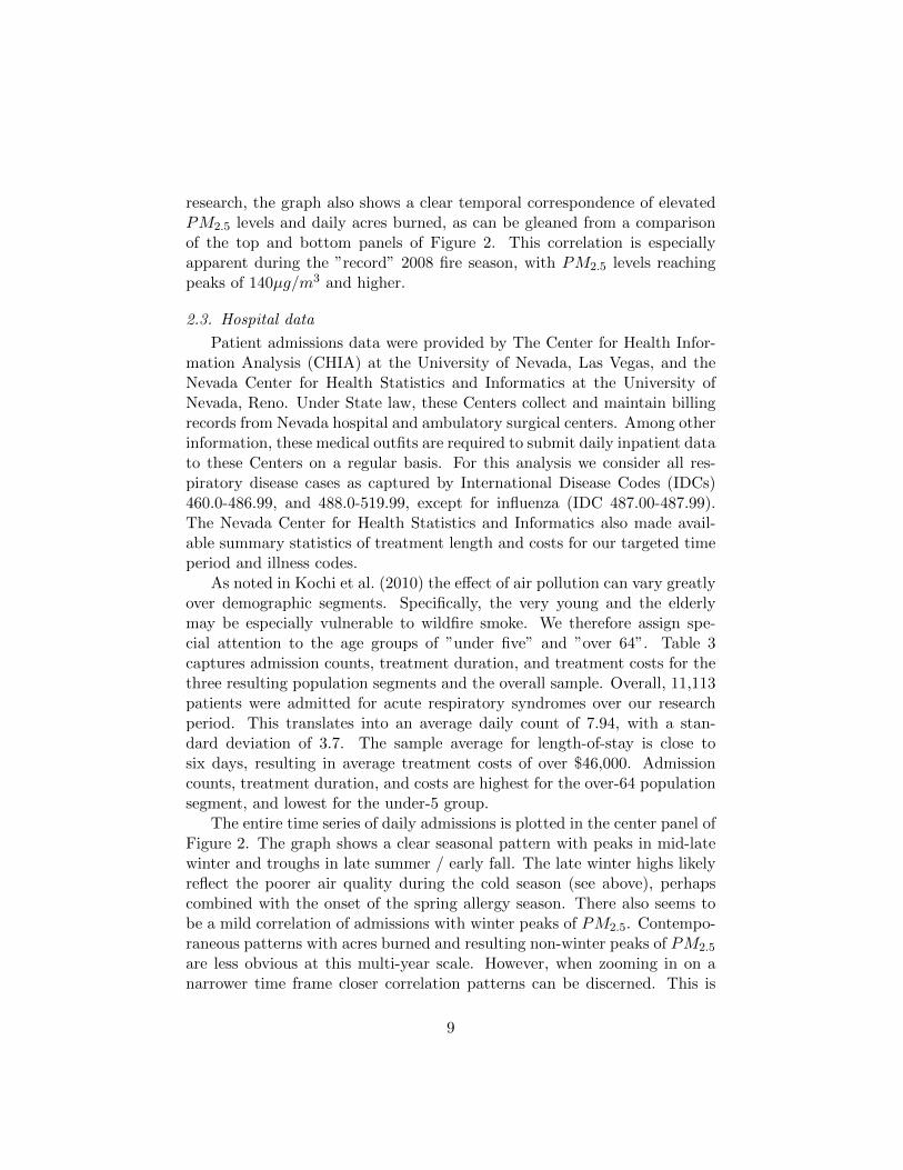
As noted in Kochi et al. (2010) the effect of air pollution can vary greatlyover demographic segments. Specifically, the very young and the elderlymay be especially vulnerable to wildfire smoke. We therefore assign spe-cial attention to the age groups of ”under five” and ”over 64”. Table 3captures admission counts, treatment duration, and treatment costs for thethree resulting population segments and the overall sample. Overall, 11,113patients were admitted for acute respiratory syndromes over our researchperiod. This translates into an average daily count of 7.94, with a stan-dard deviation of 3.7. The sample average for length-of-stay is close tosix days, resulting in average treatment costs of over $46,000. Admissioncounts, treatment duration, and costs are highest for the over-64 populationsegment, and lowest for the under-5 group.

The entire time series of daily admissions is plotted in the center panel ofFigure 2. The graph shows a clear seasonal pattern with peaks in mid-latewinter and troughs in late summer / early fall. The late winter highs likelyreflect the poorer air quality during the cold season (see above), perhapscombined with the onset of the spring allergy season. There also seems tobe a mild correlation of admissions with winter peaks of PM2.5. Contempo-raneous patterns with acres burned and resulting non-winter peaks of PM2.5

are less obvious at this multi-year scale. However, when zooming in on anarrower time frame closer correlation patterns can be discerned. This is

9

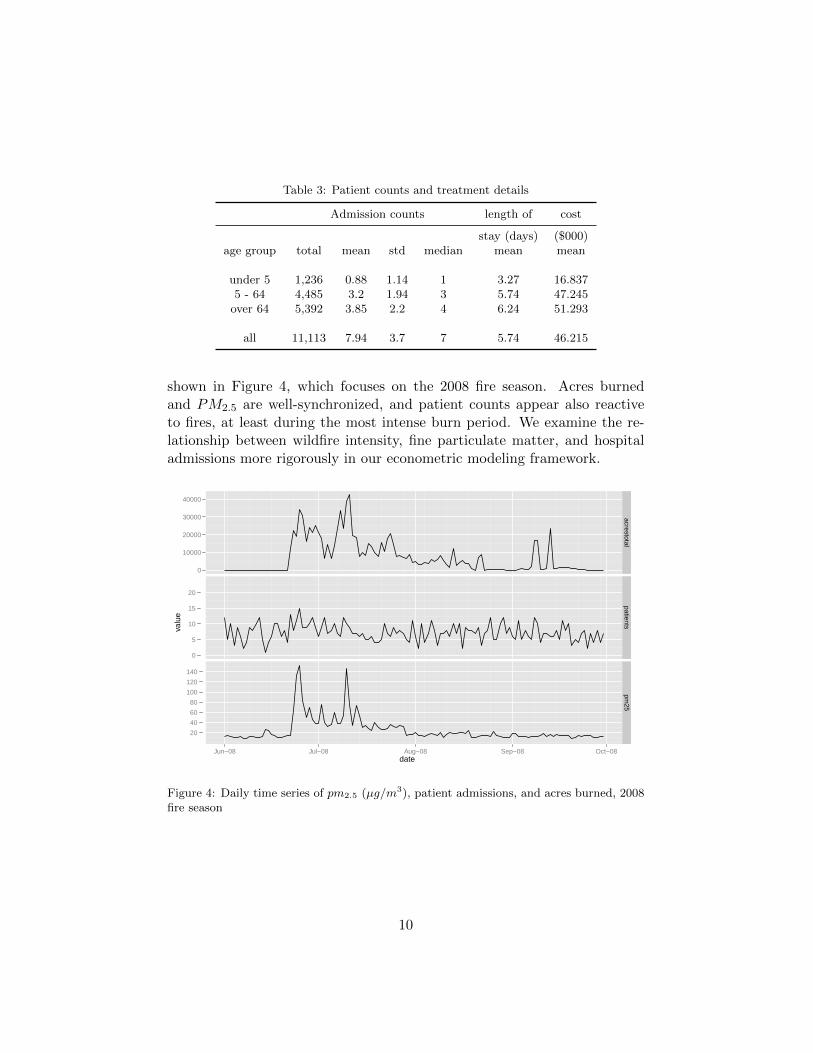
Table 3: Patient counts and treatment details

Admission counts length of cost

stay (days) ($000)age group total mean std median mean mean

under 5 1,236 0.88 1.14 1 3.27 16.8375 - 64 4,485 3.2 1.94 3 5.74 47.245

over 64 5,392 3.85 2.2 4 6.24 51.293

all 11,113 7.94 3.7 7 5.74 46.215

shown in Figure 4, which focuses on the 2008 fire season. Acres burnedand PM2.5 are well-synchronized, and patient counts appear also reactiveto fires, at least during the most intense burn period. We examine the re-lationship between wildfire intensity, fine particulate matter, and hospitaladmissions more rigorously in our econometric modeling framework.

date

valu

e

0

10000

20000

30000

40000

0

5

10

15

20

20

40

60

80

100

120

140

Jun−08 Jul−08 Aug−08 Sep−08 Oct−08

acrestotalpatients

pm25

Figure 4: Daily time series of pm2.5 (µg/m3), patient admissions, and acres burned, 2008fire season

10

3. Econometric Framework

3.1. PM2.5 model

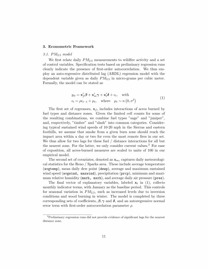
We first relate daily PM2.5 measurements to wildfire activity and a setof control variables. Specification tests based on preliminary regression runsclearly indicate the presence of first-order autocorrelation. We thus em-ploy an auto-regressive distributed lag (ARDL) regression model with thedependent variable given as daily PM2.5 in micro-grams per cubic meter.Formally, the model can be stated as

yit = x′fβ + x′mγ + x′tδ + εt, with

εt = ρεt−1 + µt, where µt ∼ n(0, σ2

) (1)

The first set of regressors, xf , includes interactions of acres burned byfuel types and distance zones. Given the limited cell counts for some ofthe resulting combinations, we combine fuel types ”sage” and ”juniper”,and, respectively, ”timber” and ”slash” into common categories. Consider-ing typical sustained wind speeds of 10-20 mph in the Sierras and easternfoothills, we assume that smoke from a given burn zone should reach theimpact area within a day or two for even the most remote fires in our set.We thus allow for two lags for these fuel / distance interactions for all butthe nearest zone. For the latter, we only consider current values.2 For easeof exposition, all acres-burned measures are scaled to units of 100 in ourempirical model.

The second set of covariates, denoted as xm, captures daily meteorologi-cal statistics for the Reno / Sparks area. These include average temperature(avgtemp), mean daily dew point (dewp), average and maximum sustainedwind speed (avgwind, maxwind), precipitation (prcp), minimum and maxi-mum relative humidity (mnrh, mxrh), and average daily air pressure (pres).

The final vector of explanatory variables, labeled xt in (1), collectsmonthly indicator terms, with January as the baseline period. This controlsfor seasonal variation in PM2.5, such as increased levels due to inversionconditions and wood burning in winter. The model is completed by threecorresponding sets of coefficients, β,γ and δ, and an autoregressive normalerror term with first-order autocorrelation parameter ρ.

2Preliminary regression runs did not provide evidence of significant lags for the nearestdistance zone.

11

3.2. Patients model

We follow existing contribution to the air pollution / health outcomeliterature (e.g. Smith et al., 2000; Clyde, 2000) and model the effect ofPM2.5 on the daily number of respiratory hospital admissions within a countdata regression framework. Specifically, we assume patient counts to followa Negative Binomial (NegBin) distribution with a log-linear parameterizedmean function, i.e.:

f (yt|λt) =Γ (yt + ν)

Γ (yt + 1) Γ (ν)

(ν

λt + ν

)ν ( λtλt + ν

)yt, with

E (yt) = λt, V (yt) =

(λt +

1

νλ2t

), and

λt = exp(z′pβ + z′mγ + z′tδ

)(2)

This corresponds to Cameron and Trivedi’s (1986) NegBin II specifi-cation with expectation λt and precision parameter ν. The parameterizedmean function λt includes three sets of regressors: zp, a vector of air pol-lutant measures, meteorological indicators zm, and temporal indicators zt.Pollutants include PM2.5, carbon monoxide (CO), and Ozone (O3). The sec-ond is another signature ingredient of biomass smoke (e.g. Fowler, 2003),and the third is another known irritant that can trigger respiratory ailments(U.S. Environmental Protection Agency, 2011). The vector of meteorolog-ical variables is identical to xm in the PM2.5 model, with the addition ofdaily minimum and maximum temperature (mintemp, maxtemp). The tem-poral variables in zt include monthly indicators (baseline = January) and anindicator for ”weekend”.3 We estimate separate admission count models forthe entire sample, and the sub-populations of ”under five” and ”over 64”.

4. Estimation results

4.1. PM2.5 model

We estimate the PM2.5 model via Full-Information-Maximum-Likelihood(FIML), which produces estimates of all slope coefficients, along with theerror correlation coefficient ρ and the variance of the i.i.d. stochastic compo-nent σ2. The results from this model are captured in Table 4. In general one

3Preliminary estimation runs did not suggest any significant lagged effects for eitherpollutants or meteorological indicators.

12

would expect positive marginal effects for all fuel / distance combinationsthat diminish over distance zones. While several of the estimated coeffi-cients for fuel / distance regressors have counter-intuitive negative signs,they generally follow the pattern of diminishing marginal effects with in-creasing distance. The timber / slash fuel category exhibits the patternmost consistent with intuition, at least beyond the 50-mile range. Whenadded over lags the marginal effects of acres burned for zones II, III, and IVare significant, positive and taper off with increasing remoteness from theimpact area.4 This is captured in Table 5. For example, an additional 100acres burned in an area dominated by timber / slash within the precedingtwo days and including the current day increases the PM2.5 count by 1.39µg/m3 for fires that occur between 50 and 100 miles from the impact area.This effect reduces to 0.30 µg/m3 for fires in zone III (101 - 250 miles), andto 0.14 µg/m3 for fires in zone IV (> 250 miles).

Table 5 also suggests that the impact of grass burns is strongest fornear-distance fires, while wildfires in the sage / juniper interface have themost detrimental impact on air quality if they occur in the 51-100 milezone. While this may reflect different dispersion patterns, it may also be anartifact of small sample counts for these fuel types for some of the distancezones.

4.2. Patients model

The patients model is estimated via Maximum Likelihood (MLE), whichgenerates estimates of the elements of the slopes in the parameterized meanfunction, and the inverse of the precision parameter ν. Estimation results forthe three NegBin models of patient admissions are captured in Table 6. Thekey finding from this analysis is the significant to highly significant effectof PM2.5 in all three population models. Furthermore, these effects differacross population segments. As shown in the first column of the table, thefull-sample model estimates an increase in expected respiratory admissionsby 0.63% due to a one µg/m3 increase in PM2.5 concentration. This effectis approximately 50% higher for young children (column three), and 24%lower for the elderly population (column five). In comparison, the othertwo pollutants, co and ozone, are not associated with significant effects onadmission counts for any of the population categories. Of the meteorological

4In distributed lag models a combined or ”cumulative” marginal effect can be computedby adding the estimated coefficients for current and lagged effects for a given regressor.See for example Koop and Tole (2004).

13

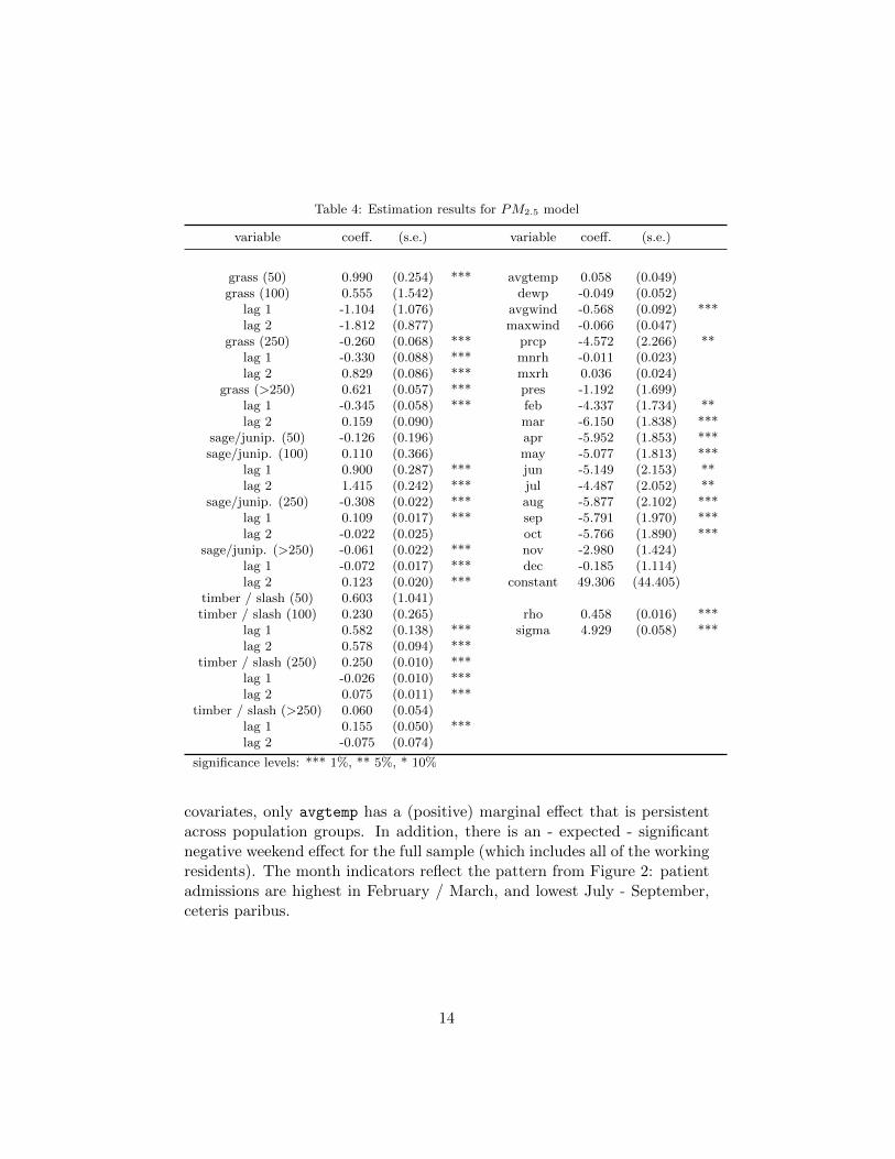
Table 4: Estimation results for PM2.5 model

variable coeff. (s.e.) variable coeff. (s.e.)

grass (50) 0.990 (0.254) *** avgtemp 0.058 (0.049)grass (100) 0.555 (1.542) dewp -0.049 (0.052)

lag 1 -1.104 (1.076) avgwind -0.568 (0.092) ***lag 2 -1.812 (0.877) maxwind -0.066 (0.047)

grass (250) -0.260 (0.068) *** prcp -4.572 (2.266) **lag 1 -0.330 (0.088) *** mnrh -0.011 (0.023)lag 2 0.829 (0.086) *** mxrh 0.036 (0.024)

grass (>250) 0.621 (0.057) *** pres -1.192 (1.699)lag 1 -0.345 (0.058) *** feb -4.337 (1.734) **lag 2 0.159 (0.090) mar -6.150 (1.838) ***

sage/junip. (50) -0.126 (0.196) apr -5.952 (1.853) ***sage/junip. (100) 0.110 (0.366) may -5.077 (1.813) ***

lag 1 0.900 (0.287) *** jun -5.149 (2.153) **lag 2 1.415 (0.242) *** jul -4.487 (2.052) **

sage/junip. (250) -0.308 (0.022) *** aug -5.877 (2.102) ***lag 1 0.109 (0.017) *** sep -5.791 (1.970) ***lag 2 -0.022 (0.025) oct -5.766 (1.890) ***

sage/junip. (>250) -0.061 (0.022) *** nov -2.980 (1.424)lag 1 -0.072 (0.017) *** dec -0.185 (1.114)lag 2 0.123 (0.020) *** constant 49.306 (44.405)

timber / slash (50) 0.603 (1.041)timber / slash (100) 0.230 (0.265) rho 0.458 (0.016) ***

lag 1 0.582 (0.138) *** sigma 4.929 (0.058) ***lag 2 0.578 (0.094) ***

timber / slash (250) 0.250 (0.010) ***lag 1 -0.026 (0.010) ***lag 2 0.075 (0.011) ***

timber / slash (>250) 0.060 (0.054)lag 1 0.155 (0.050) ***lag 2 -0.075 (0.074)

significance levels: *** 1%, ** 5%, * 10%

covariates, only avgtemp has a (positive) marginal effect that is persistentacross population groups. In addition, there is an - expected - significantnegative weekend effect for the full sample (which includes all of the workingresidents). The month indicators reflect the pattern from Figure 2: patientadmissions are highest in February / March, and lowest July - September,ceteris paribus.

14

Table 5: Marginal effects for PM2.5 model

fuel (distance) point lower upper

estimate (s.e.) (95% C.I.) (95% C.I.)

grass (50) 0.990 (0.254) 0.493 1.487 ***grass (100) -2.362 (2.767) -7.785 3.062grass (250) 0.238 (0.170) -0.096 0.572

grass (>250) 0.435 (0.090) 0.259 0.611 ***

sage / juniper (50) -0.126 (0.196) -0.511 0.259sage / juniper (100) 2.425 (0.535) 1.375 3.474 ***sage / juniper (250) -0.221 (0.030) -0.281 -0.162 ***

sage / juniper (>250) -0.010 (0.034) -0.076 0.056

timber / slash (50) 0.603 (1.041) -1.437 2.642timber / slash (100) 1.390 (0.416) 0.574 2.206 ***timber / slash (250) 0.299 (0.018) 0.263 0.335 ***

timber / slash (>250) 0.140 (0.071) 0.002 0.279 **

significance levels: *** 1%, ** 5%, * 10%

4.3. Marginal fire effects on patient admissions

So far our estimation results suggest a clear link between fire events andPM2.5 concentration in the impact area, as well as a link between the latterand patient admission counts. We combine these findings and compute apoint estimate for the direct effect of acres burned (in units of 100) for a givenfuel / distance combination on admissions by multiplying the cumulativemarginal effect from the PM2.5 model (as captured in Table 5) with themarginal PM2.5 effect from the patients model for a given population group.We derive standard errors and confidence intervals for these combined effectsvia simulation. We then translate these marginal impacts into changes intreatment costs by multiplying the expected increase in daily admissions bythe population-segment specific treatment costs as given in Table 3 above.

For this final step of our analysis we focus on the timber / slash fuel type,and on distance zones II, III, and IV, given the intuitively sound results forthese combinations from the PM2.5 model. Table 7 shows the percentagechange in daily patient admissions, and the total change in daily treatmentcosts from an additional loss of 100 acres to wildfire in timber-dominatedfuel systems. The first block of rows refers to the entire sample, while thesecond and third blocks capture, respectively, output for the ”under 4” and”over 4”’ population segments.

As is evident from the table, an additional 100 acres of burned timber

15

Table 6: Results for the respiratory admissions model

all under 4 over 64

variable coeff. (s.e) coeff. (s.e) coeff. (s.e)

constant 7.5977 (2.332) *** -3.8757 (6.576) 4.9575 (3.289)pm25 0.0063 (0.001) *** 0.0090 (0.004) ** 0.0048 (0.002) ***

co -0.0019 (0.078) -0.1767 (0.227) 0.0547 (0.110)ozone -3.0316 (2.126) -3.5829 (6.533) -0.9855 (2.958)

avgtemp 0.0113 (0.005) ** 0.0288 (0.014) ** 0.0145 (0.007) **dewp -0.0015 (0.003) 0.0205 (0.010) ** -0.0053 (0.004)

avgwind 0.0014 (0.006) 0.0050 (0.018) 0.0010 (0.009)maxwind 0.0038 (0.003) 0.0108 (0.008) 0.0032 (0.004)maxtemp -0.0050 (0.003) -0.0184 (0.009) ** -0.0010 (0.005)mintemp -0.0049 (0.004) -0.0229 (0.010) ** -0.0105 (0.005) **

prcp 0.0637 (0.111) -0.4499 (0.331) 0.1881 (0.154)mnrh 0.0008 (0.002) -0.0065 (0.005) 0.0028 (0.002)mxrh 0.0004 (0.002) 0.0024 (0.004) 0.0016 (0.002)pres -0.2131 (0.089) ** 0.1701 (0.250) -0.1540 (0.125)

weekend -0.1439 (0.023) *** -0.3198 (0.070) *** -0.1306 (0.032) ***feb 0.3573 (0.049) *** 0.4335 (0.118) *** 0.4177 (0.070) ***mar 0.2217 (0.053) *** 0.1185 (0.135) 0.2624 (0.076) ***apr -0.0742 (0.061) -0.4240 (0.164) *** 0.0077 (0.086)may -0.2005 (0.070) *** -0.9104 (0.204) *** -0.0538 (0.099)jun -0.3509 (0.081) *** -1.1357 (0.241) *** -0.1601 (0.113)jul -0.5106 (0.092) *** -1.4697 (0.282) *** -0.3843 (0.129) ***aug -0.4774 (0.088) *** -1.4792 (0.274) *** -0.3201 (0.123) ***sep -0.4197 (0.076) *** -1.3315 (0.232) *** -0.2944 (0.107) ***oct -0.3147 (0.063) *** -1.1051 (0.187) *** -0.2446 (0.090) ***nov -0.3144 (0.055) *** -1.0798 (0.162) *** -0.2209 (0.079) ***dec -0.1720 (0.048) *** -0.6689 (0.131) *** -0.0983 (0.069)

1/ν 0.0074 (0.005) 0.0066 (0.037) 0.0023 (0.010)

significance levels: *** 1%, ** 5%, * 10%

within 51-100 miles from the impact area increases patient admissions foracute respiratory illness by close to 1%, with an empirical 95% confidenceinterval of [0.3%, 1.5%]. Applying this marginal percentage effect to thesample mean of 7.94 admissions, and multiplying by the average cost perpatient ($46,215) produces a marginal increment of $3,206 in treatmentcosts. For distance zone III the expected percentage change in admissionsreduces to 0.19%, yielding an expected marginal increase in treatment costsof $696. The 100-acre marginal effect for wildfires in the > 250 mile rangeis 0.09% for changes in admission, and $329 for increased treatment costs.

16

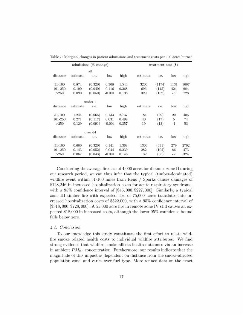
Table 7: Marginal changes in patient admissions and treatment costs per 100 acres burned

admissions (% change) treatment cost ($)

alldistance estimate s.e. low high estimate s.e. low high

51-100 0.874 (0.320) 0.308 1.544 3206 (1174) 1131 5667101-250 0.190 (0.040) 0.116 0.268 696 (145) 424 984>250 0.090 (0.050) -0.001 0.198 329 (182) -5 728

under 4distance estimate s.e. low high estimate s.e. low high

51-100 1.244 (0.666) 0.133 2.737 184 (99) 20 406101-250 0.271 (0.117) 0.031 0.499 40 (17) 5 74>250 0.129 (0.091) -0.004 0.357 19 (13) -1 53

over 64distance estimate s.e. low high estimate s.e. low high

51-100 0.660 (0.320) 0.141 1.368 1303 (631) 279 2702101-250 0.143 (0.052) 0.044 0.239 282 (102) 86 473>250 0.067 (0.043) -0.001 0.146 132 (85) -2 324

Considering the average fire size of 4,000 acres for distance zone II duringour research period, we can thus infer that the typical (timber-dominated)wildfire event within 51-100 miles from Reno / Sparks causes damages of$128,246 in increased hospitalization costs for acute respiratory syndrome,with a 95% confidence interval of [$45, 000, $227, 000]. Similarly, a typicalzone III timber fire with expected size of 75,000 acres translates into in-creased hospitalization costs of $522,000, with a 95% confidence interval of[$318, 000, $728, 000]. A 55,000 acre fire in remote zone IV still causes an ex-pected $18,000 in increased costs, although the lower 95% confidence boundfalls below zero.

4.4. Conclusion

To our knowledge this study constitutes the first effort to relate wild-fire smoke related health costs to individual wildfire attributes. We findstrong evidence that wildfire smoke affects health outcomes via an increasein ambient PM2.5 concentration. Furthermore, our results indicate that themagnitude of this impact is dependent on distance from the smoke-affectedpopulation zone, and varies over fuel type. More refined data on the exact

17

fuel composition associated with a given fire event will be needed to fullyvalidate the latter result.

While our estimated marginal hospitalization costs are non-negligible,they should best be interpreted as lower bounds of broader smoke-relatedhealth-care costs, which would include costs of treatment for patients thatsought medical assistance, but were not admitted to a local hospital. Inturn, as has been discussed elsewhere (e.g. Rittmaster et al., 2006; Kochiet al., 2010) medical treatment-related costs are likely to constitute only asmall fraction of total economic cost to the affected population, which wouldinclude components such as decreased productivity and forgone recreationalopportunities.

Overall, our results clearly suggest that even wildfires that occur hun-dreds of miles from a given population zone can, under certain wind condi-tions, induce smoke-related health damages. These potential damages needto be taken into account in the design of optimal wildfire management poli-cies.

5. References

Adamowicz, V., Dales, R., Hale, B., Hrudey, S., Krupnick, A., Lippman,M., McConnell, J., Renzi, P., 2004. Report of an expert panel to reviewthe socio-economic models and related components supporting the devel-opment of Canada-wide standards (CWS) for particulate matter (PM)and ozone to the Royal Society of Canada. Journal of Toxicology andEnvironmental Health, Part B: Critical Reviews 7, 147266.

Cameron, A.C., Trivedi, P.K., 1986. Models based on count data: Compar-ison and applications of some estimators and tests. Journal of AppliedEconometrics 1, 29–53.

Clinton, N., Scarborough, J., Yong Tian, Y., Gong, P., 2003. A GIS basedemissions estimation system for wildfire and prescribed burning. Paperpresented at the EPA 12th Annual Emission Inventory Conference, SanDiego, CA, April 29 - May 1, 2003.

Clyde, M., 2000. Model uncertainty and health effect studies for particulatematter. Environmetrics 11, 745–763.

Deeming, J., Burgan, R., Cohen, J., 1978. The National Fire Danger Rat-ing System, 1978. Technical Report INT-39. USDA Forest Service, Inter-mountain Forest and Range Experiment Station, Odgen, UT.

18

Fowler, C., 2003. Human health impacts of forest fires in the southernUnited States: a literature review. Journal of Eclogical Anthropology 7,39–63.

Holmes, T., Huggett, R.J., Westerling, A., 2008. Statistical analysis of largewildfires, in: Holmes, T., Prestemon, J., Abt, K. (Eds.), The economicsof forest disturbances: Wildfires, storms, and invasive species. Springer,pp. 59–77.

Johnston, F., Kavanagh, A., Bowman, D., Scott, R., 2002a. Bushfire smokeand asthma: an ecological study. Medical Journal of Australia 176, 535–538.

Johnston, F., Kavanagh, A., Bowman, D., Scott, R., 2002b. Serial corre-lation and confounders in time-series in air pollution studies. MedicalJournal of Australia 177, 397–398.

Kochi, I., Champ, P., Donovan, G., Loomis, J., 2011. Valuing mortality im-pacts of smoke exposure from major southern california wildfires. Workingpaper.

Kochi, I., Donovan, G., Champ, P., Loomis, J., 2010. The economic cost ofadverse health effects from wildfire smoke exposure: a review. Interna-tional Journal of Wildland Fire 19, 803–817.

Koop, G., Tole, L., 2004. Measuring the health effects of air pollution: Towhat extent can we really say that people are dying from bad air? Journalof Environmental Economics and Management 47, 30–54.

National Climatic Data Center, 2011. Climate data archive. Web site:http://www.ncdc.noaa.gov/oa/ncdc.html.

National Fire and Aviation Management, 2011. Famweb. Web site:http://fam.nwcg.gov/fam-web/.

Rittmaster, R., Adamowicz, V., Amiro, B., Pelletier, R., 2006. Economicanalysis of health effects from forest fires. Canadian Journal of ForestryResources 36, 868–877.

Smith, R., Davis, J., Sacks, J., Speckman, P., Styer, P., 2000. Regressionmodels for air pollution and daily mortality: analysis of data from Birm-ingham, Alabama. Environmetrics 11, 719–743.

19

Tham, R., Erbas, B., Akram, M., Dennekamp, M., Abramson, M., 2009.The impact of smoke on respiratory hospital outcomes during the 2002-2003 bushfire season, Victoria, Australia. Respirology 14, 69–75.

U.S. Environmental Protection Agency, 2011. Ozone - good up high, badnearby. Web site: http://www.epa.gov/oar/oaqps/gooduphigh/.

Viswanathan, S., Eria, L., Diunugala, N., Johnson, J., McClean, C., 2006.An analysis of effects of San Diego wildfire on ambient air quality. Journalof the Air and Waste Management Association 56, 56–67.

Washoe County Health District, 2011. Washoe countyair quality management reports & data. Web site:http://www.co.washoe.nv.us/health/air/aqr.html.

Western Institute for Study of the Environment, 2011. Fire tracking. Website: http://westinstenv.org/firetrack/.

20