WILEY SERIES IN PROBABILITY AND MATHEMATICAL STATISTICS

ESTABLISHED BY WALTER A . S H E W H A R T AND SAMUEL S. WlLKS Editors Vic Barnett, Ralph A. Bradley, Nicholas I. Fisher, J. Stuart Hunter, Joseph B. Kadane, David G. Kendall, Adrian F. M. Smith, Stephen M. Stigler, Jozef L. Teugels, Geoffrey S. Watson

Probability and Mathematical Statistics ADLER ■ The Geometry of Random Fields ANDERSON • The Statistical Analysis of Time Series ANDERSON * An Introduction to Multivariate Statistical Analysis,

Second Edition ARNOLD ■ The Theory of Linear Models and Multivariate Analysis BARNETT * Comparative Statistical Inference, Second Edition BERNARDO and SMITH • Bayesian Statistical Concepts and Theory BHATTACHARYYA and JOHNSON • Statistical Concepts and Methods BILL1NGSLEY • Probability and Measure, Second Edition BOROVKOV • Asymptotic Methods in Queuing Theory BOSE and MANVEL * Introduction to Combinatorial Theory CAINES • Linear Stochastic Systems CHEN • Recursive Estimation and Control for Stochastic Systems COCHRAN • Contributions to Statistics COCHRAN • Planning and Analysis of Observational Studies CONSTANTINE • Combinatorial Theory and Statistical Design COVER and THOMAS • Elements of Information Theory

*DOOB • Stochastic Processes DUDEWICZ and MISHRA • Modern Mathematical Statistics EATON • Multivariate Statistics: A Vector Space Approach ETHIER and KURTZ * Markov Processes: Characterization and Convergence FELLER * An Introduction to Probability Theory and Its Applications, Volume I,

Third Edition, Revised; Volume I I , Second Edition FULLER ■ Introduction to Statistical Time Series FULLER * Measurement Error Models GIFI ■ Nonlinear Multivariate Analysis GRENANDER • Abstract Inference GUTTORP • Statistical Inference for Branching Processes HALD ■ A History of Probability and Statistics and Their Applications before 1750 HALL * Introduction to the Theory of Coverage Processes HANNAN and DEISTLER • The Statistical Theory of Linear Systems HEDAYAT and SINHA • Design and Inference in Finite Population Sampling HOEL * Introduction to Mathematical Statistics, Fifth Edition HUBER ■ Robust Statistics IMAN and CONOVER • A Modern Approach to Statistics IOSIFESCU • Finite Markov Processes and Applications JOHNSON and BHATTACHARYYA • Statistics: Principles and Methods, Revised

Printing LAHA and ROHATGI • Probability Theory LARSON * Introduction to Probability Theory and Statistical Inference,

Third Edition MATTHES, KERSTAN, and MECKE • Infinitely Divisible Point Processes MORGENTHALER and TUKEY • Configurai Polysampling: A Route to Practical

Robustness MUIRHEAD • Aspects of Multivariate Statistical Theory OLIVER and SMITH * Influence Diagrams, Belief Nets and Decision Analysis PILZ • Bayesian Estimation and Experimental Design in Linear Regression Models PRESS • Bayesian Statistics: Principles, Models, and Applications PURI and SEN • Nonparametric Methods in General Linear Models PURI and SEN • Nonparametric Methods in Multivariate Analysis PURl, VILAPLANA, and WERTZ • New Perspectives in Theoretical and Applied

Statistics RANDLES and WOLFE • Introduction to the Theory of Nonparametric Statistics RAO * Asymptotic Theory of Statistical Inference

'Now available in a lower priced paperback edition in the Wiley Classics Library.

Probability and Mathematical Statistics (Continued) RAO • Linear Statistical Inference and Its Applications, Second Edition ROBERTSON, WRIGHT, and DYKSTRA • Order Restricted Statistical Inference ROQERS and WILLIAMS • Diffusions, Markov Processes, and Martingales, Volume

II: îto Calculus ROHATGI • Statistical Inference ROSS • Stochastic Processes RUBINSTEIN • Simulation and the Monte Carlo Method RUZSA and SZEKELY • Algebraic Probability Theory SCHEFFE ■ The Analysis of Variance SEBER • Linear Regression Analysis SEBER • Multivariate Observations SEBER and WILD • Nonlinear Regression SEN * Sequential Nonparametrics: Invariance Principles and Statistical Inference SERFLING • Approximation Theorems of Mathematical Statistics SHORACK and WELLNER ■ Empirical Processes with Applications to Statistics STAUDTE and SHEATHER • Robust Estimation and Testing STOYANOV • Counterexamples in Probability STY AN • The Collected Papers of T. W. Anderson: 1943-1985 WHITTAKER • Graphical Models in Applied Multivariate Statistics YANG • The Construction Theory of Denumerable Markov Processes

Applied Probability and Statistics ABRAHAM and LEDOLTER • Statistical Methods for Forecasting AGRESTI • Analysis of Ordinal Categorical Data AGRESTI • Categorical Data Analysis AICKIN • Linear Statistical Analysis of Discrete Data ANDERSON and LOYNES • The Teaching of Practical Statistics ANDERSON, AUQUIER, HAUCK, OAKES, VANDAELE, and

WEISBERG • Statistical Methods for Comparative Studies ARTHANARI and DODGE • Mathematical Programming in Statistics ASMUSSEN • Applied Probability and Queues

'BAILEY • The Elements of Stochastic Processes with Applications to the Natural Sciences

BARNETT • Interpreting Multivariate Data BARNETT and LEWIS • Outliers in Statistical Data, Second Edition BARTHOLOMEW • Stochastic Models for Social Processes, Third Edition BARTHOLOMEW and FORBES • Statistical Techniques for Manpower Planning BATES and WATTS • Nonlinear Regression Analysis and Its Applications BECK and ARNOLD • Parameter Estimation in Engineering and Science BELSLEY • Conditioning Diagnostics: Collinearity and Weak Data in Regression BELSLEY, KUH, and WELSCH • Regression Diagnostics: Identifying Influential

Data and Sources of Collinearity BHAT • Elements of Applied Stochastic Processes, Second Edition BHATTACHARYA and WAYMIRE • Stochastic Processes with Applications BIEMER, GROVES, LYBERG, MATHIOWETZ, and SUDMAN • Measurement

Errors in Surveys BLOOMFIELD • Fourier Analysis of Time Series: An Introduction BOLLEN • Structural Equations with Latent Variables BOX • R. A. Fisher, the Life of a Scientist BOX and DRAPER • Empirical Model-Building and Response Surfaces BOX and DRAPER • Evolutionary Operation: A Statistical Method for Process

Improvement BOX, HUNTER, and HUNTER • Statistics for Experimenters: An

Introduction to Design, Data Analysis, and Model Building BROWN and HOLLANDER • Statistics: A Biomédical Introduction BUCKLEW • Large Deviation Techniques in Decision, Simulation, and Estimation BUNKE and BUNKE • Nonlinear Regression, Functional Relations and Robust

Methods: Statistical Methods of Model Building BUNKE and BUNKE • Statistical Inference in Linear Models, Volume I CHAMBERS • Computational Methods for Data Analysis CHATTERJEE and HADI • Sensitivity Analysis in Linear Regression CHATTERJEE and PRICE • Regression Analysis by Example, Second Edition

*Now available in a lower priced paperback edition in the Wiley Classics Library.

Applied Probability and Statistics (Continued) CHOW * Econometric Analysis by Control Methods CLARKE and DISNEY • Probability and Random Processes: A First Course with

Applications, Second Edition COCHRAN * Sampling Techniques, Third Edition COCHRAN and COX • Experimental Designs, Second Edition CONOVER * Practical Nonparametric Statistics, Second Edition CONOVER and IMAN • Introduction to Modern Business Statistics CORNELL ■ Experiments with Mixtures, Designs, Models, and the Analysis of Mixture

Data, Second Edition COX • A Handbook of Introductory Statistical Methods COX • Planning of Experiments CRESSIE • Statistics for Spatial Data DANIEL • Applications of Statistics to Industrial Experimentation DANIEL * Biostatistics: A Foundation for Analysis in the Health Sciences, Fourth

Edition DANIEL and WOOD • Fitting Equations to Data: Computer Analysis of Multifactor

Data, Second Edition DAVID • Order Statistics, Second Edition DAVISON ■ Multidimensional Scaling DEGROOT, FIENBERG, and KADANE • Statistics and the Law

*DEMING * Sample Design in Business Research DILLON and GOLDSTEIN • Multivariate Analysis: Methods and Applications DODGE • Analysis of Experiments with Missing Data DODGE and ROMIG * Sampling Inspection Tables, Second Edition DOWDY and WEARDEN • Statistics for Research, Second Edition DRAPER and SMITH * Applied Regression Analysis, Second Edition DUNN * Basic Statistics: A Primer for the Biomédical Sciences, Second Edition DUNN and CLARK • Applied Statistics: Analysis of Variance and Regression, Second

Edition ELANDT-JOHNSON and JOHNSON • Survival Models and Data Analysis FLEISS * The Design and Analysis of Clinical Experiments FLEISS • Statistical Methods for Rates and Proportions, Second Edition FLEMING and HARRINGTON • Counting Processes and Survival Analysis FLURY ■ Common Principal Components and Related Multivariate Models FRANKEN, KÖNIG, ARNDT, and SCHMIDT • Queues and Point Processes GALLANT • Nonlinear Statistical Models GIBBONS, OLK1N, and SOBEL • Selecting and Ordering Populations: A New

Statistical Methodology GNANADESIKAN • Methods for Statistical Data Analysis of Multivariate

Observations GREENBERG and WEBSTER ■ Advanced Econometrics: A Bridge to the Literature GROSS and HARRIS • Fundamentals of Queueing Theory, Second Edition GROVES • Survey Errors and Survey Costs GROVES, BIEMER, LYBERG, MASSEY, NICHOLLS, and WAKSBERG •

Telephone Survey Methodology GUPTA and PANCHAPAKESAN • Multiple Decision Procedures: Theory and

Methodology of Selecting and Ranking Populations GUTTMAN, WILKS, and HUNTER • Introductory Engineering Statistics, Third

Edition HAHN and MEEKER • Statistical Intervals: A Guide for Practitioners HAHN and SHAPIRO • Statistical Models in Engineering HALD * Statistical Tables and Formulas HALD • Statistical Theory with Engineering Applications HAND * Discrimination and Classification HEIBERGER • Computation for the Analysis of Designed Experiments HELLER • MACSYMA for Statisticians HOAGLIN, MOSTELLER, and TUKEY • Exploratory Approach to Analysis of

Variance HOAGLIN, MOSTELLER, and TUKEY • Exploring Data Tables, Trends and Shapes HOAGLIN, MOSTELLER, and TUKEY • Understanding Robust and Exploratory

Data Analysis HOCHBERG and TAMHANE • Multiple Comparison Procedures HOEL • Elementary Statistics, Fourth Edition

Continued on back end papers 'Now available in a lower priced paperback edition in the Wiley Classics Library.

Forecasting with Dynamic Regression Models

Forecasting with Dynamic Regression Models

ALAN PANKRATZ DePauw University Greencastle, Indiana

Wiley-Interscience Publication JOHN WILEY & SONS INC. New York • Chichester • Brisbane • Toronto • Singapore

A NOTE TO THE READER This book has been electronically reproduced from digital information stored at John Wiley & Sons, Inc. We are pleased that the use of this new technology will enable us to keep works of enduring scholarly value in print as long as there is a reasonable demand for them. The content of this book is identical to previous printings.

In recognition of the importance of preserving what has been written, it is a policy of John Wiley & Sons, Inc., to have books of enduring value published in the United States printed on acid-free paper, and we exert our best efforts to that end.

Copyright © 1991 by John Wiley & Sons, Inc.

All rights reserved. Published simultaneously in Canada.

Reproduction or translation of any part of this work beyond that permitted by Section 107 or 108 of the 1976 United States Copyright Act without the permission of the copyright owner is unlawful. Requests for permission or further information should be addressed to the Permissions Department, John Wiley & Sons, Inc.

Library of Congress Cataloging in Publication Data: Pankratz, Alan, 1944-

Forecasting with dynamic regression models / Alan Pankratz. p. cm. — (Wiley series in probability and mathematical

statistics. Applied probability and statistics, ISSN 0271-6356) "A Wiley-Interscience publication." Includes bibliographical references and index. ISBN 0-471-61528-5 1. Time-series analysis. 2. Regression analysis. 3. Prediction

theory. I. Title. II. Series. QA280.P368 1991 519.5'5-dc20 91-12484

CIP

10 9 8 7 6 5

To Aaron Mark Dietrich and Sherith Hope Laura

Contents

Preface

Chapter 1 Introduction and Overview 1.1 Related Time Series, 1 1.2 Overview: Dynamic Regression Models, 7 1.3 Box and Jenkins' Modeling Strategy, 15 1.4 Correlation, 17 1.5 Layout of the Book, 21

Questions and Problems, 22

Chapter 2 A Primer on ARIMA Models 2.1 Introduction, 24 2.2 Stationary Variance and Mean, 27 2.3 Autocorrelation, 34 2.4 Five Stationary ARIMA Processes, 39 2.5 ARIMA Modeling in Practice, 49 2.6 Backshift Notation, 52 2.7 Seasonal Models, 54 2.8 Combined Nonseasonal and Seasonal Processes, 57 2.9 Forecasting, 59 2.10 Extended Autocorrelation Function, 62 2.11 Interpreting ARIMA Model Forecasts, 64

Questions and Problems, 69

viii CONTENTS

Case 1 Federal Government Receipts (ARIMA) 72

Chapter 3 A Primer on Regression Models 82 3.1 Two Types of Data, 82 3.2 The Population Regression Function (PRF) with One Input, 82 3.3 The Sample Regression Function (SRF) with One Input, 86 3.4 Properties of the Least-Squares Estimators, 88 3.5 Goodness of Fit (R2), 89 3.6 Statistical Inference, 92 3.7 Multiple Regression, 93 3.8 Selected Issues in Regression, 96 3.9 Application to Time Series Data, 103

Questions and Problems, 113

Case 2 Federal Government Receipts (Dynamic Regression) 115

Case 3 Kilowatt-Hours Used 131

Chapter 4 Rational Distributed Lag Models 147 4.1 Linear Distributed Lag Transfer Functions, 148 4.2 A Special Case: The Koyck Model, 150 4.3 Rational Distributed Lags, 156 4.4 The Complete Rational Form DR Model and Some

Special Cases, 163 Questions and Problems, 165

Chapter 5 Building Dynamic Regression Models: Model Identification 167 5.1 Overview, 167 5.2 Preliminary Modeling Steps, 168 5.3 The Linear Transfer Function (LTF) Identification Method, 173 5.4 Rules for Identifying Rational Distributed Lag Transfer

Functions, 184 Questions and Problems, 193 Appendix 5A The Corner Table, 194 Appendix 5B Transfer Function Identification Using Prewhitening

and Cross Correlations, 197

CONTENTS ix

Chapter 6 Building Dynamic Regression Models: Model Checking, Reformulation, and Evaluation 202

6.1 Diagnostic Checking and Model Reformulation, 202 6.2 Evaluating Estimation Stage Results, 209

Questions and Problems, 215

Case 4 Housing Starts and Sales 217

Case 5 Industrial Production, Stock Prices, and Vendor Performance 232

Chapter 7 Intervention Analysis 253

7.1 Introduction, 253 7.2 Pulse Interventions, 254 7.3 Step Interventions, 259 7.4 Building Intervention Models, 264 7.5 Multiple and Compound Interventions, 272

Questions and Problems, 276

Case 6 Year-End Loading 279

Chapter 8 Intervention and Outlier Detection and Treatment 290 8.1 The Rationale for Intervention and Outlier Detection, 291 8.2 Models for Intervention and Outlier Detection, 292 8.3 Likelihood Ratio Criteria, 299 8.4 An Iterative Detection Procedure, 313 8.5 Application, 315 8.6 Detected Events Near the End of a Series, 319

Questions and Problems, 320 Appendix 8A BASIC Program to Detect AO, LS, and IO

Events, 321 Appendix 8B Specifying IO Events in the SCA System, 322

Chapter 9 Estimation and Forecasting 324

9.1 DR Model Estimation, 324 9.2 Forecasting, 328

Questions and Problems, 340 Appendix 9A A BASIC Routine for Computing the

Nonbiasing Factor in (9.2.24), 340

X CONTENTS

Chapter 10 Dynamic Regression Models in a Vector ARMA Framework 342

10.1 Vector ARMA Processes, 342 10.2 The Vector AR (IT Weight) Form, 345 10.3 DR Models in VAR Form, 346 10.4 Feedback Check, 349 10.5 Check for Contemporaneous Relationship and

Dead Time, 354 Questions and Problems, 356

Appendix 357 Table A Student's / Distribution, 357 Table B x2 Critical Points, 359 Table C F Critical Points, 360

Data Appendix 362

References 376

Index 381

Preface

Single-equation regression models are one of the most widely used statistical forecasting tools. Over the last two decades many ideas relevant to regression forecasting have arisen in the time series literature, starting with the first edition of Box and Jenkins' text, Time Series Analysis: Forecasting and Control, Holden-Day (1976). Those who apply regression methods to time series data without knowledge of these ideas may miss out on a better understanding of their data, better models, and better forecasts.

This book is a companion volume to my earlier text, Forecasting with Univariate Box-Jenkins Models: Concepts and Cases, Wiley (1983), where I present the Box-Jenkins modeling strategy as applied to ARIMA models. There is more to Box and Jenkins than ARIMA models. They also discuss "combined transfer function-disturbance" models, or what I call dynamic regression models. The purpose of the present text is to pull together recent time series ideas in the Box-Jenkins tradition that are important for the informed practice of single-equation regression forecasting. I pay special attention to possible intertemporal (dynamic) patterns —distributed lag re-sponses of the output series (dependent variable) to the input series (indepen-dent variables), and the autocorrelation patterns of the regression disturb-ance.

This book may be used as a main text for undergraduate and beginning graduate courses in applied time series and forecasting in areas such as economics, business, biology, political science, engineering, statistics, and decision science. It may be used in advanced courses to supplement theoreti-cal readings with applications. And it can serve as a guide to the construction and use of regression forecasting models for practicing forecasters in business and government.

Special features of this book include the following:

• Many step-by-step examples using real data, including cases with multiple inputs, both stochastic and deterministic.

• Emphasis on model interpretation.

xi

xii PREFACE

• Emphasis on a model identification method that is easily applied with multiple inputs.

■ Suggested practical rules for identifying rational form transfer functions. • Emphasis on feedback checks as a preliminary modeling step. • Careful development of an outlier and intervention detection method,

including a BASIC computing routine. • A chapter linking dynamic regression models to vector ARMA models. • Use of the extended autocorrelation function to identify ARIMA models.

While there are other books that cover some of these ideas, they tend to cover them briefly, or at a fairly high level of abstraction, or with few supporting applications. I present the theory at a low level, and I show how these ideas may be applied to real data by means of six case studies, along with other examples within the chapters. Several additional data sets are provided in the Data Appendix. The examples and cases are drawn mainly from economics and business, but the ideas illustrated are also applicable to data from other disciplines.

Those who read the entire text will notice some repetition; I realize that many readers will read only selected chapters and cases, and that most won't already know the contents of this book before they read, so I have tried to repeat some key ideas. I hope my readers will learn enough of the main ideas and practices of dynamic regression forecasting to feel more comfortable and be more insightful when doing their own data analysis, criticizing their own procedures and results, moving ahead to more advanced literature and pract-ices, and when moving back to less advanced methods.

I have successfully used a majority of the material in this book with undergraduates, most of whom have had just one course in statistics. I assume that readers have been exposed to the rudiments of probability, hypothesis testing, and interval estimation. A background in regression meth-ods is helpful but not required; Chapter 3 is an introduction to the fundamen-tals of regression. I use matrix algebra in a few places, primarily Chapter 10, but a knowledge of matrix algebra is not required to understand the main ideas in the text. For many readers the most difficult part of the text may be the use of backshift notation. If you are one of those readers, to you I say (1) it's only notation, (2) learning to use it is easier than learning to ride a bicycle, and (3) it's immensely useful.

As you read this book, I hope you find parts that are interesting, informa-tive, and helpful. When you do, you should be as grateful as I am to Gregory Hudak, Brooks Elliott, and an anonymous reviewer who provided many excellent comments on a draft of the manuscript. I am also grateful to Fran Cappelletti for his perceptive comments on parts of the manuscript. I wish I could also blame shortcomings and undetected errors on these people, but I can't; I didn't take all of their advice, and any problems you encounter are my responsibility. Various members of the DePauw University Computer

PREFACE xiii

Center staff, my colleagues in the Department of Economics and Manage-ment, and those faculty and administrators responsible for DePauw summer grants all facilitated my work in various ways. Paul Koch graciously provided some of the data used in Case 5.

Anyone who knows Bea Shube knows of her competence and wisdom. I was fortunate in starting this project under her editorial guidance. Kate Roach was informative, encouraging, and patient while taking on this project in editorial midstream. Rosalyn Farkas and Ernestine Franco provided out-standing editorial and production assistance.

All of the computational results shown in this text were produced by the SCA System software (developed in collaboration with George E. P. Box, Mervin E. Müller, and George C. Tiao). Contact: Scientific Computing Associates, Lincoln Center, Suite 106, 4513 Lincoln Avenue, Lisle, IL, 60532, (708) 960-1698. Similar results may be obtained with various other packages, including several from Automatic Forecasting Systems, Inc., P.O. Box 563, Hatboro, PA, 19040, (215) 675-0652; SAS Institute Inc., Box 8000, Cary, NC, 27511, (919) 467-8000; or Gwilym Jenkins & Partners Ltd., Parkfield, Greaves Road, Lancaster LAI 4TZ, U.K.

My wife Charity didn't read or type anything this time, but she was her usual good natured and supportive self as I showed all the symptoms of Author's Disease. Though I mentioned it dozens of times, I don't think my children are much aware that I have written another book. But then, they are teenagers, or were while I was writing, with far more important things to think about. Maybe they will notice that this book is dedicated to them, with pride and affection.

ALAN PANKRATZ Greencastle, Indiana June 1991

CHAPTER 1

Introduction and Overview

1.1 RELATED TIME SERIES

Comedian George Carlin has noticed that "If there were no such thing as time, everything would happen all at once." Of course, there is such a thing as time, and everything doesn't happen all at once. Events occurring at one time are often related to other events occurring at other times.

Our daily lives are full of examples. For instance, several years ago my son had a severe headache. The pain was so bad that we took him to the local hospital where a physician gave him some pain medication. After 10 minutes my son felt a little better. After 20 minutes he felt much better. After 30 minutes he felt little pain and was able to sleep. My son's pain relief at any given time was related to the receipt of pain medication at an earlier time.

As another example, suppose a state passes a law requiring all car occu-pants to wear seat belts as of January 1. Some people who have not worn belts might start wearing them immediately on January 1; others might start wearing them only after many reminders and many days have passed; still others might wear belts only after being arrested or fined; and some might never wear belts. Our ability to understand the effect of the seat belt law, and our ability to forecast the effect of passing a similar law in another state, depend on a correct understanding of the role of time in this situation.

The same holds true in many other contexts: We may misunderstand the effects of public or private policy actions, or the nature of physical, chemical, or biological mechanisms, if we do not understand the special role played by time in the relationship between time-ordered variables. And our ability to forecast time-ordered variables may be impaired if we don't understand the time structure of relationships between variables.

Studying such interrelationships using time-ordered data is called time series analysis. The goal in time series analysis is to find a useful way (a "model") to express a time-structured relationship among some variables or events. We may then evaluate this relationship or we may forecast one or more of the variables. That is the focus of this book.

1

INTRODUCTION AND OVERVIEW

Shipments 44000

3 8 0 0 0 time '

1 13 25 37 49

Figure 1.1 Valve shipments, January 1984-May 1988.

Let's consider three more examples of related time series. In each example we have sequences of observations on two separate time-ordered variables that are (possibly) related to each other.

1.1.1 Example 1: Valve Shipments and Orders

Figure 1.1 shows 53 time-ordered (from left to right) monthly observations of the number of small valves shipped by a manufacturer. The data are recorded from January 1984 through May 1988. Figure 1.2 shows 53 corre-sponding time-ordered monthly observations of the volume of orders for this valve to be shipped during the same month.

The volume of valve shipments is recorded at the end of the month, while

3 2 0 0 0

1 13 25 37 49

Figure 1.2 Valve orders, January 1984-May 1988.

RELATED TIME SERIES

Table 1.1 Partial Listing of Valve Shipments and Orders Data Date January 1984 February 1984 March 1984

April 1988 May 1988 June 1988

Shipments 39,377 39,417 39,475

43,299 42,687

Orders 35,862 34,165 33,127

39,331 40,203 38,916

the volume of valve orders for that month is recorded at the start of the month. Thus, the volume of shipments can differ from the volume of orders since the manufacturer accepts late orders, and some orders may be canceled. Since the volume of valve orders is recorded one month earlier than the corresponding shipments, there are 54 observations of orders (rather than 53), and the orders data are recorded through June 1988; Figure 1.2 shows only the first 53 values. The full data set is listed in the Data Appendix as Series 1 (shipments) and Series 2 (orders).

Table 1.1 is a partial listing of the data. We said that the shipments and orders observations are "corresponding." That is, the data occur in time-ordered pairs; each value of shipments for a given month (recorded at the end of the month) is paired with a corresponding value of orders for the same month (recorded at the start of the month). For example, as shown in Table 1.1, the manufacturer began March 1984 with orders for 33,127 valves to be shipped that month, but ended March 1984 with 39,475 valves actually shipped during that month.

It is reasonable to think that the volume of shipments during a given month might be related to the volume of orders on the books at the start of that month. Indeed, inspection of Figures 1.1 and 1.2 suggests that higher shipment levels are associated with higher order levels, and lower shipment levels with lower order levels. Thus knowledge of the volume of orders on the books at the start of a given month might help us to forecast the volume of shipments for that month.

1.1.2 Example 2: Interrupted Saving Rate Series Figure 1.3 shows 100 time-ordered observations of the saving rate (saving as a percent of income) in the United States from the first quarter (I) of 1955 to the fourth quarter (IV) of 1979. These data are listed in the Data Appendix as Series 3. The observation for 1975 II (the 82nd observation) stands out from the rest of the data: It is markedly higher than both earlier and later

4 INTRODUCTION AND OVERVIEW

Saving Rate 10

82 time >

Figure 1.3 U.S. saving rate, 1955 1-1979 IV.

observations. This jump up at the 82nd observation could be just unexplain-able random variation in the data. However, during that quarter Congress passed a law granting a one-time tax rebate. According to at least one economic theory (the permanent income hypothesis), such a rebate will lead to a temporary increase in the saving rate. The saving rate series may have been interrupted by a known event (at 1975 II) whose effect can be explained.

We can represent the tax rebate event by creating a binary indicator variable (a series consisting of only 0's or l's) to reflect the "on-off " nature of the rebate. We define this series as having two parts: a set of zeros that stand for "no rebate during this quarter" and a set of ones that stand for "rebate during this quarter." This gives us a set of 100 time-ordered and paired observations for the two series. Table 1.2 is a partial listing of these

Table 1.2 Partial Listing of Saving Rate Data and Tax Rebate Binary Indicator Variable Date Saving Rate

(%) Binary Indicator

Variable

1955 1 4.9 0

1975 I 1975 II 1975 III

6.4 9.7 7.5

0 1 0

1979 IV 3.5

RELATED TIME SERIES 5

series. The binary indicator variable has the value 0 throughout, except at 1975 II when the tax rebate took place; then it has the value 1.0.

This example is similar to Example 1. However, in this example only the values of the saving rate series are observed; the values of the binary indicator variable are constructed by us rather than observed. In the previous example both the valve shipments and valve orders data were observed, not con-structed.

1.1.3 Notation In the next example we illustrate some helpful notation that we will use throughout this book. The letter Y stands for a variable whose values may depend on one or more other variables or events. In our earlier examples Y is the level of headache pain, the number of car occupants wearing seat belts, the monthly volume of valve shipments, or the saving rate. The letter X stands for a variable that might affect Y. Thus X could be the amount of pain medication received, a binary indicator variable representing the pres-ence or absence of a seat belt law, the volume of valve orders, or a binary indicator variable representing the presence or absence of the tax rebate.

The letter / is used as a subscript to indicate time: Y, and X, stand for variables whose possible values are time ordered. Thus, we have t -1,2,3, . . . , where the value of t indicates the place of the corresponding observation (either actual or possible) in the data sequence; that is, Yt is the first observation, Y& is the 69th observation, and so forth. Of course, / can correspond to a particular date. For example, for monthly data it could be that / = 1 corresponds to December 1979, t = 2 corresponds to January 1980, and so on.

Sometimes it is useful to write the time subscript as t - 1, / - 2, t - 3 , . . . , or as t + 1, t + 2, t + 3 , . . . . The meaning of the positive and negative signs is fairly obvious: A negative refers to a time period before period t, and a positive refers to a time period after period t. For example, if we have daily data and X, corresponds to Wednesday, then X,-t corresponds to the prior Tuesday, and X,-2 corresponds to the prior Monday, while X,+ l corresponds to the next Thursday, and Xl+2 corresponds to the next Friday, and so forth.

1.1.4 Example 3: Sales and Leading Indicator Figure 1.4 shows 150 time-ordered observations (denoted Yt) of the sales of a certain product. Figure 1.5 shows 150 corresponding time-ordered obser-vations (denoted X,) of a leading indicator variable that might be useful in forecasting the sales data. Each horizontal axis is measured in time units (t = 1,2,3,.. .); each vertical axis is measured in units of Y, or X,. Table 1.3 is a partial listing of these data. For time period r = 1, Yt = 200.1, and X{ = 10.01; for t = 2,Y2 = 199.5, and X2 = 10.07; and so forth. The full sales and

INTRODUCTION AND OVERVIEW

2 7 0

Y _

1 9 0 -+-t i m e -

Figure 1.4 Product sales.

leading indicator data sets are listed in the Data Appendix as Series 4 and Series 5, respectively.

The idea here is that changes in X, may signal current or later (especially later) changes in Y, since X, is supposedly a leading indicator for Y,. That is, maybe movements in Y, reflect movements in X,, or Ar,_,, or X,.2, and so forth. Another way to say this is that changes in X, may lead to changes in Y„ y,+ i, Y,+2, and so forth. Figures 1.4 and 1.5 suggest that this might be so because higher (lower) values of X, seem to be associated with higher (lower) values of Y,. We will consider in detail the possible relationship between X, and Y, in this example in Chapters 5, 6, 9, and 10.

1.1.5 Inputs, Output, and Models In this book we consider situations with one time series variable to be forecast or predicted (denoted Y,), and one or more time series variables (denoted

tine Figure 1.5 Leading indicator.

OVERVIEW: DYNAMIC REGRESSION MODELS

Table 1.3 Partial Listing of Sales and Leading Indicator Data

t = Time Y, = Sales X, = Indicator 1 200.1 10.01 2 199.5 10.07 3 199.4 10.32

149 262.2 13.77 150 262.7 13.40

Xi,„ X2,i,. . .) that might help to forecast the future movements or explain the past movements of Y,. For convenience we will call variable Y, the output and variables XlJ,X2„ . . . the inputs. In Examples 1, 2, and 3 we had just one input in each case —the valve orders input, the binary tax rebate input, and the leading indicator input, respectively. (Chapter 3 and Cases 2, 3, 5, and 6 in this book show examples with multiple inputs.) As in Example 2, an input may be constructed rather than observed. Thus inputs can be stochastic (having some random variation, like the valve orders data in Example 1) or deterministic (having no random variation, like the constructed rebate versus no rebate binary variable in Example 2).

Our goal is to use the available data to build a statistical model that represents the relationship between the output (V,) and the inputs (Xij, X2.,,...). We may then use this model to forecast the output series, test a hypothesis about the relationship between the output and the inputs, or assess the effect of an event, including a policy action, on the output. In the latter case we may simply want to understand the historical effect of a past event on the output. Or, we may want to predict the possible effect of a similar future event on the output.

1.2 OVERVIEW: DYNAMIC REGRESSION MODELS

In this book we focus on a family of statistical models called dynamic regres-sion (DR) models. A DR model states how an output (Y,) is linearly related to current and past values of one or more inputs (Xu, X2j,. ..). It is usually assumed that observations of the various series occur at equally spaced time intervals. (However, a model in which we allow for slightly unequally spaced data is shown in Case 2.) While the output may be affected by the inputs, a crucial assumption is that the inputs are not affected by the output. This means that we are limited to single-equation models.

INTRODUCTION AND OVERVIEW

Y ï Y t i m e > t - 2 t - 1 t t l m e '

Figure 1.6 Possible time-lagged relationships between V, and X,.

These ideas are illustrated schematically in Figure 1.6. Note that X, and Y, are measured at equally spaced time intervals. The solid arrows show that it is acceptable in a single-equation DR model to have statistical effects going from current and past values of X, (X„ X,-u X,~2, . . .) to the current value of Y,. However, it is not appropriate to have effects (the dashed line arrows) going from current or past values of Y, (Y,-lt y,_2,. . .) to the current X,.

I assume that most readers have some exposure to the basic ideas of correlation and regression analysis. Section 1.4 reviews the idea of corre-lation; Chapter 3 reviews regression. To introduce the idea of a DR model, we first consider how we might apply ordinary regression analysis to Ex-amples 1, 2, and 3 in Section 1.1. (An ordinary regression model, when applied to time series data, is a simple example of a DR model.)

1.2.1 Regression One way to link the valve shipments data to the valve orders data (or the saving rate data to the constructed binary variable, or the sales data to the leading indicator) is to estimate the ordinary regression model

Y, = C + v0X, + N, (1.2.1)

where C is the population intercept, a parameter to be estimated; u0 is the population slope coefficient, also a parameter to be estimated; and N, is a stochastic disturbance term. The disturbance is present because we cannot expect variation in the input(s) to explain all of the variation in the output. The disturbance represents variation in the output that is not associated with movements in the input(s).

Equation (1.2.1) is a simple example of a DR model with one input. Y, is the output such as valve shipments, and X, is the input such as valve orders. According to (1.2.1), valve shipments and valve orders are content-

OVERVIEW: DYNAMIC REGRESSION MODELS 9

f (a t )

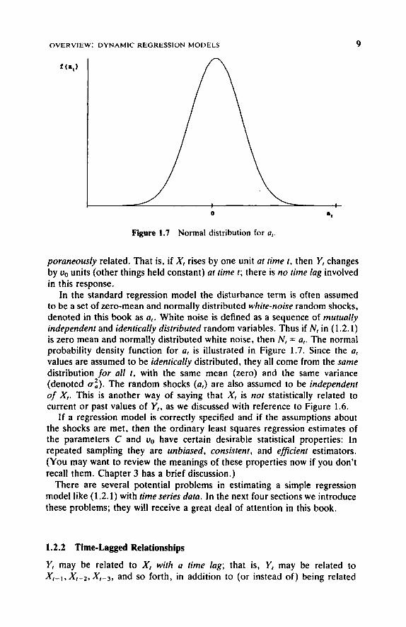
Figure 1.7 Normal distribution for a,.

poraneously related. That is, if X, rises by one unit at time t, then Y, changes by u0 units (other things held constant) at time t; there is no time lag involved in this response.

In the standard regression model the disturbance term is often assumed to be a set of zero-mean and normally distributed white-noise random shocks, denoted in this book as a,. White noise is defined as a sequence of mutually independent and identically distributed random variables. Thus if N, in (1.2.1) is zero mean and normally distributed white noise, then N, = a,. The normal probability density function for a, is illustrated in Figure 1.7. Since the a, values are assumed to be identically distributed, they all come from the same distribution for all t, with the same mean (zero) and the same variance (denoted al). The random shocks (a,) are also assumed to be independent of X,. This is another way of saying that X, is not statistically related to current or past values of Y,, as we discussed with reference to Figure 1.6.

If a regression model is correctly specified and if the assumptions about the shocks are met, then the ordinary least squares regression estimates of the parameters C and v0 have certain desirable statistical properties: In repeated sampling they are unbiased, consistent, and efficient estimators. (You may want to review the meanings of these properties now if you don't recall them. Chapter 3 has a brief discussion.)

There are several potential problems in estimating a simple regression model like (1.2.1) with time series data. In the next four sections we introduce these problems; they will receive a great deal of attention in this book.

1.2.2 Time-Lagged Relationships

Y, may be related to X, with a time lag; that is, Y, may be related to X,-i, Xr-2, X,-3, and so forth, in addition to (or instead of) being related

10 INTRODUCTION AND OVERVIEW

to X,. For example, instead of Equation (1.2.1), suppose that a correct statement of how Y, is related to X, is

y, = C+«*,*, +u ,* , - , + u2ÀV-2 + N, (1.2.2)

We use C as a generic symbol for a constant; thus C may have a different value in (1.2.2) than it has in (1.2.1). If (1.2.2) is the correct specification of the relationship between the output and the input, estimating the par-ameters in (1.2.1) instead of (1.2.2) can lead to a variety of problems. For example, in estimating (1.2.1) we lose useful information about the roles of X,-i and X,-2 in explaining movements in Y,. Thus our estimate of the residual variance (the variance of N,) will be larger than necessary, and our forecasts are likely to be less accurate than they could be. Further, the estimate of the coefficient v0 attached to the included variable (A",) in (1.2.1) will be biased and inconsistent //the excluded variables (A^i and X,-2) are correlated with the included variable (X,). This problem could easily occur with time series data since such data (the input series, in this case) tend to be ««//-correlated; that is, X, tends to be correlated with its own past values X,-i, X,-2, . . . .

In this book we study methods for identifying the nature of the time-lagged relationship between an output and current and past values of one or more inputs. These methods are designed to help us include all relevant earlier values of the inputs, and exclude all irrelevant ones. These methods are discussed especially in Chapters 5 through 7 and Cases 4 through 6.

1.2.3 Feedback from Output to Inputs

Another potential problem in the use of ordinary regression is that there may be feedback from Y, to X,. This is illustrated in Figure 1.6 by the dashed arrows. For example, in addition to Equation (1.2.1) or (1.2.2), there might also be another relationship between X, and Y,, expressed as

X, = C* + WiY.-i + M, (1.2.3)

where C* is a constant; w, is a slope coefficient parameter; and M, is a stochastic disturbance. When an input X, responds in some way to current or past values of Y„ as in (1.2.3), this is called feedback from Y, to X,.

If feedback is present, the disturbance N, in (1.2.1) or (1.2.2) is correlated with one or more of the input variables on the right side of those equations. Estimating (1.2.1) or (1.2.2) using ordinary single-equation regression meth-ods when feedback is present leads to inconsistent estimates of the par-ameters: As the sample size grows, the repeated sampling distributions of the estimates collapse onto values that differ from the parameters by unknown amounts. Even if we had all data from the population, applying the usual regression formulas to the data would not give us estimates equal to the