wimax capacity white paper - pudn.comread.pudn.com/downloads167/doc/766153/wimax-capacity_3.pdf ·...

WiMAX Capacity White Paper

Notice The information in this manual is subject to change without notice. All statements, information and recommendations in this manual are believed to be accurate, but are presented without warranty of any kind, expressed or implied. Users must take full responsibility for their use of any products. No part of this publication may be reproduced or transmitted in any form or by any means, electronic or mechanical, including photocopying and recording, or by any information storage or retrieval system, without prior written consent from SR Telecom Inc. SR TELECOM, SYMMETRY, SYMMETRYONE and SYMMETRYMX are trademarks of SR Telecom Inc. All rights reserved 2006. All other trademarks are property of their owners. Information subject to change without notice. © 2006, SR Telecom Inc. All rights reserved. August 2006 Printed in Canada

WHITE PAPER 033-100743-001,ISSUE 1 2

Table of Contents

1 ABSTRACT................................................................................................... 6

2 PROTOCOL MODEL .................................................................................... 8

2.1 DATA/CONTROL PLANE..............................................................................9 2.2 MANAGEMENT PLANE ................................................................................9

3 PHYSICAL LAYER ..................................................................................... 10

3.1 CHANNEL SIZE........................................................................................10 3.2 OFDM...................................................................................................11 3.3 FRAME AND SYMBOL SIZE........................................................................14 3.4 PREAMBLES............................................................................................14

3.4.1 Synchronization .........................................................................14 3.4.2 Ranging .....................................................................................15 3.4.3 Midambles .................................................................................16

3.5 SUB-CHANNELS.......................................................................................16 3.6 MINIMUM ALLOCATION UNIT .....................................................................17

3.6.1 Downlink....................................................................................17 3.6.2 Uplink ........................................................................................18

3.7 ADAPTIVE MODULATION/CODING AND POWER CONTROL.............................19 3.8 DIVERSITY..............................................................................................20

3.8.1 Space-Time Coding (STC) ........................................................20 3.8.2 MIMO.........................................................................................20

3.9 ADAPTIVE ANTENNA SYSTEM (AAS) .........................................................21

4 MEDIA ACCESS CONTROL LAYER ......................................................... 22

4.1 MAC HEADER ........................................................................................22 4.1.1 Sub headers ..............................................................................24

4.2 CHANNEL USAGE MAPS...........................................................................26 4.2.1 Frame Control Header...............................................................26 4.2.2 Downlink Map............................................................................26 4.2.3 Uplink Map.................................................................................28 4.2.4 Downlink and Uplink Channel Descriptors.................................28

4.3 BANDWIDTH REQUESTS ...........................................................................29 4.3.1 Contention .................................................................................29 4.3.2 Polling........................................................................................31 4.3.3 Piggyback..................................................................................32

5 CHANNEL BANDWIDTH CALCULATION................................................. 33

6 QOS ............................................................................................................ 36

6.1 CONSTANT BIT RATE SERVICES................................................................36 6.2 VARIABLE BIT RATE SERVICES .................................................................37 6.3 BEST EFFORT SERVICES..........................................................................38 6.4 SHARING NON-GUARANTEED BANDWIDTH .................................................38 6.5 OVER-SUBSCRIPTION ..............................................................................39

7 CAPACITY SCENARIOS............................................................................ 42


7.1 BROADBAND DATA-ONLY.........................................................................42 7.2 MIXED VOICE AND BROADBAND ................................................................43

8 SUMMARY.................................................................................................. 45


List of Figures

FIGURE 1 - IEEE 802.16 PROTOCOL REFERENCE MODEL.......................................... 8 FIGURE 2 - MAC PDU FORMATS ........................................................................... 22 FIGURE 3 - GENERIC MAC HEADER FORMAT........................................................... 23 FIGURE 4 - DOWNLINK BANDWIDTH CALCULATION SEQUENCE.................................... 33 FIGURE 5 - UPLINK BANDWIDTH CALCULATION SEQUENCE ........................................ 34 FIGURE 6 - WIMAX CHANNEL BANDWIDTH SPREADSHEET MODEL............................. 35 FIGURE 7 – AGGREGATE CHANNEL BANDWIDTH PARTITIONING .................................. 39 FIGURE 8 - ALLOCATING NETWORK BANDWIDTH ....................................................... 41

1


Abstract This white paper discusses factors influencing system capacity in IEEE 802.16 networks. IEEE 802.16, commonly known by its industry forum moniker of WiMAX, is a wireless protocol intended for establishing metropolitan area networks that supply broadband data and voice services. The present standards document, IEEE 802.16-2004 as amended by IEEE 802.16-2005, is more accurately regarded as a family of distinct physical layer standards sharing a common media access layer. This family of physical layers includes separate standards for single-carrier, and two distinct orthogonal multi-carrier physical layers. Historically the OFDM physical layer was the primary focus of the initial effort to develop a protocol suitable for non-line-of-sight (NLOS) stationary radio station operation. Succeeding development of the OFDMA physical layer focused on adding features to support low-speed mobile operation. In this white paper, we will confine the capacity discussion to the OFDM physical layer in order to avoid a lengthy discussion of the additional complications that mobility introduces; including handover and dynamic cell occupancy. Capacity for mobile applications will be an important topic for a later white paper. The objective of this white paper is to better understand WiMAX system capacity. But first, what do we mean by the “capacity” of a WiMAX system? Simply put, the system capacity refers to the number of connections that the wireless channel can support without unduly degrading the data services carried on the channel.1. We focus on the wireless channel rather than other system resources because normally the airlink is the most expensive and therefore the controlling system element related to capacity in wireless access networks. Operators care deeply about the system capacity because of the nature of wireless access network deployments. WiMAX access networks are often deployed in point-to-multipoint cellular fashion where a single base station provides wireless coverage to a collection of subscriber stations within the coverage area. The base station in turn is linked to external wide area networks via wired, fiber, or wireless point-to-point backhaul infrastructure. Normally, the radio spectrum that is available to a deployment is a scarce and often expensive resource. During the planning phase of a deployment, once an operator has determined the radio spectrum channel size for each base station, the next question becomes: how many data connections can the channel support? The question is doubly important since it is often prohibitively expensive to later overlay additional wireless capacity into the same coverage area. Further, it is central to understanding how may base stations are required for a deployment region. And without a firm understanding of the system capacity an operator has no way of estimating the recovery time for the up-front costs of deploying the access network. Understanding the system capacity is therefore key to deploying a commercially successful access network.

1 As we will see, each WiMAX connection carries data traffic characterized by a set of QoS parameters, so that a set of connections has an associated aggregate total bandwidth. The capacity of the system can therefore equivalently be thought of in terms of the aggregate total bandwidth required to support a set of connections.


In wired networks, such as legacy voice, the capacity of a channel (trunk) is intuitively obvious because each active voice conversation requires fixed dedicated bandwidth (e.g. t = 64 kbits/s plus a small signaling overhead) and the capacity is simply the number of conversations that the channel (trunk) bandwidth, T, can support: capacity = (T / t). In a WiMAX wireless channel, the situation is considerably more complex as we shall see. To begin with, the channel is not necessarily of fixed size but can vary with time as environmental conditions change. This is particularly relevant in NLOS channels. Also, a WiMAX channel can be configured in a number of different ways depending on operator preferences, regulatory constraints, and performance requirements. Many of these configuration choices affect the channel capacity, often in non-obvious ways. Finally, the nature of mixed application broadband data services defies easy classification of an “average” connection. Accurate capacity analysis therefore presupposes detailed specification of the number and type of the data services sharing the channel. As we will see, the manner in which the traffic is mapped onto the WiMAX channel’s QoS model also affects the capacity. The capacity of a WiMAX system therefore depends on environmental conditions, configuration, and the nature of the data traffic that is transported by the system. The structure of this white paper begins with a discussion of the 802.16 protocol model. Next we examine the system capacity at the physical layer including a discussion of the overhead needed to support the wireless channel. Moving up the protocol stack we next look at the capacity at the media access layer and examine the overhead introduced there. We next examine the WiMAX QoS model and discuss how the mapping of data services influences the system capacity. Bringing this information together, we next illustrate the resultant system capacity that arises in several hypothetical deployment scenarios. The white paper concludes with a brief summary of the main points.


2 Protocol Model The IEEE 802.16 protocol is a member of the IEEE 802 family of standards and addresses the media access and physical layers. The protocol reference model is shown in Figure 1. Figure 1 - IEEE 802.16 Protocol Reference Model A standard protocol-layering model is used. MAC peers communicate by sending/receiving data to/from the PHY layer. The PHY layers communicate via the 802.16 airlink. In the point-to-multipoint mode of operation, a base station transmits on the downlink channel to a collection subscriber stations by broadcasting the data to the stations that then select data that is addressed to them. Each subscriber station communicates with a single base station and a collection of subscriber stations share an uplink channel for transmitting to the base via a multiple access scheme that is controlled by the base.


2.1 Data/Control Plane User data flows into an 802.16 node at the MAC CS SAP and is passed to the underlying PHY layer at the PHY SAP. The PHY layer then transports the data over the 802.16 airlink. When we speak of the capacity of an 802.16 system we are referring to capability to pass the user data that flows vertically through the Data/Control Plane shown in the figure.

2.2 Management Plane Although not part of the standard, management traffic can also enter the system via the Management Plane. Some of this traffic may be destined for remote stations and is transported via the PHY layer via the airlink. Strictly speaking, capacity analysis should account for management traffic as part of the overall system overhead. However, because management traffic is ordinarily a negligible portion of the overall traffic load, it will mostly be ignored in this white paper.


3 Physical Layer WiMAX protocol adds overhead to user traffic starting with the physical layer, which transmits MAC PDUs to physical layer peers over the airlink. This section presents the overhead incurred at the PHY layer including mandatory and optional elements. Variable factors including adaptive modulation and code rate are discussed. The physical (PHY) layer takes MAC PDUs input at the PHY SAP and arranges them for transport over the airlink. The WiMAX protocol adds overhead to user traffic starting with the physical layer, which transmits to peer physical layers over the airlink. This section presents the overhead incurred at the PHY layer including mandatory and optional elements. Variable factors including adaptive modulation and code rate are discussed.

3.1 Channel Size A basic understanding of a WiMAX system’s capacity begins with knowing how much radio spectrum is available. The available radio spectrum ultimately constrains the size of the channels in frequency bandwidth. The channel size in turn fixes the raw capacity of the channel – double the channel size and the capacity doubles (albeit range in general will decrease). The 802.16 MAC/PHY standard attempts to avoid constraining the carrier frequency (“below 11 GHz”) for OFDM/OFDMA radios and places very general limits on the channel size (from 1.25 to 20 MHz). There are currently no worldwide spectrum allocations for WiMAX systems. The obvious issue is interoperability between hardware implementations, which the WiMAX Forum has addressed by developing equipment profiles that specify licensed/unlicensed carrier frequency and channel sizes, as well as long lists of interrelated mandatory and optional features from the 802.16 standard. WiMAX certification of compliant implementations is based on these profiles in order to insure basic interoperability between vendors. Many large operators have strong motivation, either competitive or regulatory, to operate in licensed spectrum bands. Of the available bands in the global patchwork of regulated spectrum the licensed 3.5 GHz ITU FDD blocks are the most widely available. For this reason, the majority of initial WiMAX equipment has been certified for use in the 3.5 GHz band. The available profile channel sizes are integer multiples of 1.75 MHz (1.75, 3.5, 7 MHz). The channel size is driven by the size of an operator’s allocation from their country’s regulator. For example, assuming cell reuse of one between four-sector base stations, an operator needs 14+14 MHz for 3.5 MHz channels and 7+7 MHz for 1.75 MHz channels. Oftentimes clustered base station deployments will require even more spectrum to increase the reuse factor and mitigate interference between coverage cells.


3.2 OFDM In Orthogonal Frequency Division Multiplexing, the occupied spectrum is broken up into many discrete narrowband channels known as “sub carriers” (alternatively known as “tones”). Each data carrier is modulated over a symbol time that is inversely related to the carrier frequency spacing so that sub carriers have minimal mutual interference between them. In this sense the sub carriers are “orthogonal” or independent from one another. The capacity of each sub carrier depends on the modulation order, which can be BPSK (1 bit per sub carrier), QPSK (2 bits per sub carrier), 16QAM (4 bits per sub carrier), or 64QAM (6 bits per sub carrier) in the case of the OFDM PHY. In general more power is required for using higher order modulation in order to achieve the same range performance. In the OFDM PHY there are 256 sub carriers spanning the sampling spectrum which is defined as:

Eq. 1) Fs = FLOOR(n · BW / 8000) · 8000 ,

Where n is the sampling factor, a constant dependent on the channel size, and BW is the channel size in units of Hz. The number of sub carriers corresponds to the size of the FFT/IFFT used to receive and transmit the OFDM symbols. To reduce the complexity of the digital processing algorithms it is desirable to use FFT sizes that are powers of 2. For channels in the 3.5 GHz band the licensed channels are multiples of 1.75 MHz and n = 8/7. For a channel width of 3.5 MHz the sampling spectrum is 4.0 MHz. The 256 sub carriers are equally distributed across the sampling spectrum implying a spacing of:

Eq. 2) ∆f = Fs/256 .

For example ∆f = Fs/256 = 15,625 Hz for a 3.5 MHz channel. Notice that changing the channel width changes both the sub carrier spacing and the symbol time. This implies a range of practical channel sizes for fixed applications but quickly becomes unworkable for mobile applications where the design approach of scaling the FFT size to the channel width is used with the OFDMA PHY. In order to provide increased inter-channel interference margin and ease the radio filtering constraints, not all of the 256 sub carriers are energized. There are 28 lower and 27 upper “guard” sub carriers plus the DC sub carrier that are never energized. Of the 256 total sub carriers therefore, only 200 are used which leaves a total occupied spectrum of ∆f · 200 = 3.125 MHz for a 3.5 MHz channel. This example implies a raw, occupied bandwidth efficiency of 89% (3.125/3.5 = 89%), but the number varies for other channel bandwidths and sampling factors. This is the first example we have encountered of what can be considered to be channel overhead that decreases the channel capacity, in this case it is required by design to improve the channel quality when adjacent spectrum is occupied.


Not all of the 200 occupied sub carriers are used to carry data traffic. There are eight pilot sub carriers that are dedicated for channel estimation purposes, leaving 192 data sub carriers for user and management traffic. In order to calculate the raw channel capacity it is useful to understand how many bits each data sub carrier can carry. The raw sub carrier capacity, before taking out the overhead added by redundant error correction bits, is given by the modulation order: 6 bits/sub carrier for 64QAM, 4 bits/sub carrier for 16 QAM, and so on. For example, a channel able to support 64QAM modulation could send six bits for each data carrier per symbol. But how long is a symbol? As we noted, the orthogonality of the sub carriers is achieved by maintaining an inverse relationship between the sub carrier spacing and the symbol time. So the useful symbol time is just the inverse of the sub carrier spacing:

Eq. 3) Tb = 1/∆f.

For example, a 3.5 MHz channel has a useful symbol time of 1/15625 = 64 us. However for multi-path channels, we must make allowances for variable delay spread and time synchronization errors. In OFDM, this is accomplished by repeating a fraction of the last portion of the useful symbol time and appending it to the beginning of the symbol for a resulting symbol time of:

Eq. 4) Ts = Tb + G · Tb,

Where G is a fraction:

Eq. 5) G = 1/2m, m = {2,3,4,5}.

The repeated symbol fraction is called the “cyclic prefix”. Larger cyclic prefix implies increased overhead (decreased capacity since the cyclic prefix carries no new information) but larger immunity to ISI from multi-path and synchronization errors. For a 3.5 MHz channel the useful symbol time is 64 us and the minimum total symbol time is Ts = 64 us + 64/32 us = 66us. The raw channel capacity per symbol is:

Eq. 6) Craw = 192 · k / Ts,

Where k is the bits per symbol for the modulation being used. Assuming 64QAM modulation (6 bits per symbol): 192 data sub carriers x 6 bits/sub carrier / 66 us = 17.45 Mbps. But in any practical wireless system we can expect to have occasional errors introduced by imperfect transmission, the airlink, or imperfect detection. The solution is to send redundant bits with the information bits in each symbol to aid in error detection and correction, a technique known as Forward Error Correction (FEC). In the OFDM PHY FEC is done using a combination of a Reed-Solomon outer code combined with a convolutional inner code. Adding redundant bits adds overhead and


reduces the channel capacity. The design goal is to balance the added overhead against the improvement in link performance and residual error rate. The useful capacity of the combined 192 data sub carriers therefore depends on the overall coding rate as given by the following table reproduced from the standard (Table 215 in IEEE 802.16-2004). Table 1 - Mandatory Channel Coding Per Modulation Notice that the modulation rates are designed so that an FEC coded block just fits in one symbol time when all 192 sub carriers are used. For instance for 64QAM, 144 Bytes = 1152 bits / 6 bits/symbol = 192 sub carriers. The useful channel capacity per symbol is:

Eq. 7) C = Craw x OCR,

Where OCR is the overall coding rate given in the table. For example, for a 3.5 MHz channel the useful channel capacity per symbol assuming the highest rate modulation and coding is: C = 17.45 Mbps x 3/4 = 13.1 Mbps.2

It is useful to summarize the discussion of the channel capacity is terms of the spectral efficiency. Spectral efficiency is expressed in units of bits per second per Hz and is obtained by dividing the channel capacity by the channel width:

Eq. 8) E = C / BW.

We can see that our 3.5 MHz channel has a spectral efficiency (so far) up to 13.1 Mbps / 3.5 MHz = 3.74 b/s/Hz. The spectral efficiency is a useful figure of merit to keep in mind because it lets you quickly calculate the capacity for other channel sizes that WiMAX supports.

2 By now at least some readers must be wondering what happened to the often-hyped 75 Mbps channel capacity for WiMAX? Taking the very largest channel size, 20 MHz, highest coding rate, and minimum cyclic prefix, the raw channel size using equation 6 is: Craw = 192 x 6 b/sub carrier / 11.3 us = 102.0 Mbps. The useful channel size from equation 7 is: C = Craw x ¾ = 76.5 Mbps. Of course we have said nothing about the (short) range of such a hypothetical channel, and we should be aware that this is before taking out other PHY and MAC layer overhead that, as we will see, is significant. To be blunt, talking about 75 Mbps WiMAX channels for MAN applications is about as meaningful as quoting the top end speed marked on the speedometer of a family minivan.


3.3 Frame and Symbol Size So far we have been concerned with the combined capacity of the sub carriers referenced to the OFDM symbol time. In fact, the symbols are not sent in an endless stream but are formatted into a TDMA frame with a whole number of symbols per frame. Since the symbol time varies with channel width there is no way to have a whole number of symbols fit into a fixed frame length in every case. This means that there can be a small gap at the end of each frame that is unused. This overhead, amounting to less than one symbol period in a frame, depends on the selected frame size and channel width and is of greatest impact for shorter frame lengths. In the OFDM PHY specification the allowed frame sizes are: Tf = {2.5, 4, 5, 8, 10, 12.5, 20 ms}. For a 3.5 MHz channel width with a 1/8 cyclic prefix, the symbol length is 72 us. Assuming a 10 ms frame length the whole number of symbols per frame is:

Eq. 9) N = FLOOR(Tf / Ts)

Where Tf is the frame length. In this case, N = FLOOR(10ms/72us) = 138 symbols. The gap at the end of the frame is therefore Tf – (138 x Ts) = 64 us, equivalent to about 0.6% reduction is the sustainable channel capacity. This discussion assumes that Frequency Division Duplex (FDD) channels are used, which uses separate spectrum for the transmit and receive channels. WiMAX also supports Time Division Duplex (TDD) channels, which uses the same spectrum for the receive and transmit channels. TDD is used primarily in unlicensed spectrum deployments. With TDD, the transmit and receive frames are adjustable in length and there is a mandatory guard time gap between them which can increase the overhead slightly. The constraint that the transmit and receive frames must have a whole number of symbols remains.

3.4 Preambles

3.4.1 Synchronization

Receivers need a way of synchronizing to the beginning of the TDMA frame and symbol time. On the downlink (base station talking to a subscriber station) synchronization is provided by a fixed preamble pattern of bits that is transmitted at the beginning of each frame. Since the preamble transmits no actual data its presence reduces the channel capacity. The downlink preamble takes two OFDM symbols out of each frame. Therefore, after accounting for transmission gaps at the end of the frame, the overhead is increased by 2/N where N is the number of whole symbols in a frame. Obviously this impacts shortest frame lengths most since N is smaller. For our example 3.5 MHz channel with a 1/8 cyclic prefix and a 10ms frame, the downlink preamble overhead amounts to 2/138 = 1.4%.


The uplink on the other hand is shared between a collection of subscriber stations and the base station receiver similarly needs to synchronize to each subscriber station transmitter when they begin to transmit a “burst” of data consisting of one or more consecutive symbols in a frame.3 This requires each subscriber station to prepend a preamble to the beginning of each burst. The preambles occupy one symbol at the beginning of each and every burst. The overhead this presents is variable depending on the burst size in terms of the number of symbols. This is our first example of overhead that depends on the type of user traffic that is being carried by the channel. In the worst case, subscriber stations are sending bursts of very short data requiring only a single symbol per frame. For example, referring to the coding table, suppose each subscriber station was using 64QAM-3/4 and sent 108 Bytes (uncoded) or less in each burst, that is one symbol’s worth of data assuming all data carriers are used. In this case, the overhead amounts to an alarming 50% because each one symbol burst would be sent with a one-symbol preamble.4 Fortunately many types of user traffic have characteristically longer burst sizes or can be buffered to group data requests together to form longer bursts.

3.4.2 Ranging

In a WiMAX system consisting of a base station communicating with a collection of subscriber stations at different ranges, we need a method compensating for the variable transit delay over the airlink so that the base station can coordinate selective use of the uplink and avoid receiving symbols that overlap in time. This is accomplished by measuring the distance (delay) between each subscriber station and their base station. The goal is to make each subscriber station appear to be collocated with the base station in terms of the transmission alignment. The details of the methods used (part of the “initial ranging” and “periodic ranging” processes) are unimportant to our capacity discussion except that periodically, a base station will allocate one or more uplink symbols for listening to new subscriber stations joining the network and reporting their delay compensation value and other data needed to communicate with the base station. These ranging opportunities are allocated on the uplink assuming a two-symbol preamble. The total allocation is therefore at least three symbols long.5 How often the base station listens for ranging information is configurable but in steady state an allocation every few hundred OFDM frames is reasonable.6 The overhead is therefore normally quite negligible and affects the uplink frame only.

3 In the 802.16 OFDM PHY protocol a burst is a consecutive group of symbols in the time axis by all of data sub carriers in the frequency axis. For the uplink, if optional sub-channels are supported, multiple simultaneous bursts can be supported by dividing the data sub carriers into groups. A burst is confined to a TDMA frame and must use the same channel parameters such as modulation and coding, transmitted power, etc., during the burst. 4 Granted 108 Bytes is not a lot of data but the example is not entirely academic, many compressed VoIP implementations generate packet sizes less than 100 Bytes every 10 to 20 ms. Aggregating the packets together implies increasing end-to-end latency that may not be acceptable 5 It could be longer at the base station’s discretion to allow for more subscriber stations to join at once with smaller chance of colliding with each other’s requests. Normally this is only an issue for initial base station startup where there could be a large number of subscriber stations trying to join at once. 6 Section 10.1 in IEEE 802.16-2004 defines the maximum interval between initial ranging opportunities as 2 seconds.


Once a subscriber station has joined a network, it periodically needs to refresh the ranging values (“periodic ranging” process). This is configurable and done on a per subscriber station basis but similarly requires negligible added overhead because it is performed relatively infrequently. To summarize, preambles required for receiver synchronization and ranging are examples of required overhead at the PHY layer. For now, simply note that the uplink has higher overhead than the downlink because of the shared nature of the channel and that burst preamble overhead can be significant.

3.4.3 Midambles

Midambles are allowed for OFDM PHY bursts under certain circumstances. The goal is to improve channel estimation particularly in mobile scenarios. For the uplink, midambles, if enabled, are inserted every 8, 16, or 32 data symbols. For the downlink, midambles are optional if downlink sub-channels are implemented as specified in the IEEE 802.16e-2005 amendment. Because the focus of midambles is on mobility where channel estimation is more dynamic, we will ignore their overhead contribution here.

3.5 Sub-channels The OFDM PHY allows the uplink channel to be subdivided into 16 sub-channels in order to allow subscriber stations to concentrate their transmission power into fewer data sub carriers in each symbol.7 This also lets multiple subscriber stations share the channel simultaneously, which increases the flexibility (and scheduler complexity) for efficiently using the uplink channel. Support of sub-channels by subscriber stations is optional. Sub-channels affect the channel capacity indirectly by changing the minimum allocation unit on the uplink. The standard supports sub-channel grouping in powers of two so that a subscriber station can transmit in 1, 2, 4, 8, or all 16 sub-channels (the default). The smallest allocation unit is one sub-channel, which consists of 192/16 = 12 sub carriers in frequency by one OFDM symbol in time. In that case the coded and uncoded block size is 1/16 of the value shown in the coding table. In general, the coded and uncoded block sizes shown in the coding table are reduced by a fraction determined by the number of allocated sub-channels divided by 16. This allows very granular data allocations on the uplink, which can improve the airlink utilization by matching the allocation to the amount of data being sent. For instance, without sub-channels a subscriber station using 64QAM-2/3 code rate has an uncoded minimum allocation unit of 96 Bytes. If the subscriber station needs to send 6 Bytes in a frame then 90 Bytes of the allocation are wasted. However if a single sub-channel is allocated the uncoded minimum allocation unit is 96 x 1/16 = 6 Bytes. The allocation perfectly matches the data payload in that case.

7 Sub-channels can be useful for balancing the uplink and downlink link margins since ordinarily subscriber stations, compared to the base station, have much lower radiated power capability due to cost and antenna constraints. Regulatory power density limits, as always, must be observed when transmitting in fewer sub-channels.


Sub-channels therefore influence a capacity analysis depending on the size of the payload in relationship to the minimum allocation unit. In order to make an estimate of the amount of wasted capacity (overhead) in an allocation we need to have an idea of the average payload size which in turn depends on the types of data applications supported by the subscriber stations.

3.6 Minimum Allocation Unit One of the strengths of OFDM technology is its ability to send very small amounts of information using as few as a single data sub carrier for one symbol time. For example, using the highest order modulation (64QAM), a single data sub carrier could be used to send as few as six bits at a time. The channel usage is therefore, at least in principle, highly granular. In terms of the channel capacity this granularity helps reduce the amount of wasted bandwidth in sending packets over the channel, because the allocation can be closely fitted to the size of the packet. In that case the aggregate capacity of the channel increases because it can be used more efficiently. However, there are restrictions on how the 802.16 OFDM PHY organizes the data sub carriers into Minimum Allocation Units (MAU). The MAU is the smallest two-dimensional quantum of frequency and time that can be allocated for sending information across the channel. In the OFDM PHY the MAU’s useful capacity (Bytes) is variable and depends on the chosen modulation and coding according to the following.

Eq. 10) SIZEOF(MAU) = FLOOR(Nc * Nsc * OCR / 16) , where

Nc = coded block size in Bytes (see Table 1), and Nsc = number of allocated sub-channels (1..16) for the uplink or 16 for the downlink.8

3.6.1 Downlink

The downlink does not support sub-channels for the OFDM PHY with the current baseline specification.9 The downlink MAU is therefore one symbol by all (192) data sub carriers. The second column in Table 1 shows the MAU size in number of Bytes, which varies with coding and modulation. This size allows each symbol to carry exactly one FEC block, which protects the integrity of the data over the wireless channel.

8 To be completely accurate, each burst should have one Byte subtracted from the total size because of the tail bits required to flush the convolutional coder. For instance, if an uplink burst consisted of only one MAU, the total size would be one Byte less than calculated in the equation. 9 Downlink sub-channel support in PMP deployments was recently added in the IEEE 802.16e-2005 amendment (see 8.3.5.1.1) for improved frequency reuse, lower overhead, and mobility support. In remains to be seen how widely this feature will be adopted for fixed applications, which is the focus of this white paper.


For the downlink, the base station has sole usage and control of the channel. Later we will see that there are packing and fragmentation features at the MAC layer that can be used to fit the size of the packets to be sent to the MAU. In addition, the base station scheduler has considerable freedom in arranging the packets to be sent into a burst, which can be shared, by multiple subscriber stations. However there can be cases where the amount of data to be sent in a burst just spills over a MAU boundary, and in those cases a nearly empty MAU is sent, representing additional channel overhead. Clearly, the additional overhead represented by fractionally occupied downlink MAUs is variable. In order to estimate the impact of the additional overhead on the downlink from unused portions of the MAU we need to know something about the packet size and the modulation distributions. A worst-case estimate of the additional overhead would be to assume that each burst has one additional unused MAU associated with it. For the downlink the number of bursts depends on number of separate channel profiles in use but will typically be less than four within the time span of a TDMA frame.

3.6.2 Uplink

The uplink supports optional sub-channels for the OFDM PHY. By default, when sub-channels are not used, the MAU is the same as the downlink: one symbol by all data sub carriers. The second column in Table 1 shows the MAU size in number of Bytes in that case which varies with coding and modulation. This size allows each symbol to carry exactly one FEC block. When sub-channels are implemented, the MAU is as shown in the table but divided by the number of sub-channels allocated to the subscriber station. For example in the case of 64QAM-2/3, if a single sub-channel is allocated to a subscriber station, the MAU is 96 Bytes / 16 = 6 Bytes. For the uplink, the base station controls access to the channel that is shared between multiple subscriber stations. Only a single subscriber station can transmit on a (sub)channel at once. As with the downlink, packing and fragmentation features at the MAC layer that can be used to fit the size of the packets to be sent to the MAU. But because an uplink burst can only be used by a single subscriber station, there is less opportunity for the base station to optimally fit the amount of uplink data to the MAU quanta. Mitigating this disadvantage is that the MAU is smaller when sub-channels are supported. However there can be cases where the amount of data to be sent in a burst just spills over a MAU boundary, and in those cases a nearly empty MAU is sent, representing additional channel overhead.


As with the downlink, the additional overhead represented by fractionally occupied MAUs is variable. In order to estimate the impact of the additional overhead on the uplink from unused portions of the MAU we need to know something about the packet size and the modulation distributions. A worst-case estimation of the additional overhead would be to assume that each burst has one additional unused MAU associated with it. For the uplink the number of bursts depends on number of active subscriber stations in a frame. The number of uplink bursts per frame will generally be higher than the downlink for this reason.

3.7 Adaptive Modulation/Coding and Power Control In wired networks the channel impairments tend to be constant or at least very slowly varying. Wireless networks in contrast, especially those that support non-line-of-sight (NLOS) communication, are well known for rapidly fluctuating channel conditions even when the transmitter and receiver are stationary. Broadly speaking, the lower the modulation and coding rate, and the higher the transmitted power, the more channel fading a system can tolerate and still maintain a link at a constant error level. It is desirable therefore to be able to dynamically change the transmitted power and coding rate to best match the channel conditions at the moment in order to continually support the highest capacity channel possible. WiMAX systems, controlled by the base stations, support adaptive modulation and coding on both the downlink and uplink and adaptive power control on the uplink. Adaptive modulation and coding is relevant to our capacity discussion because it changes the size of the raw channel. Referring to the channel coding table, the uncoded channel size varies by a factor of nine between the highest and lowest modulation. This means that the channel capacity can vary by nearly an order of magnitude depending on link conditions! This potentially presents a real challenge to predicting the overall system capacity. Fortunately, in properly designed real systems consisting of more than a few 10’s of stationary subscriber stations, the overall distribution of modulation and code rates tends to be relatively stable.10 For analysis purposes, what is important is knowledge of what the modulation distribution is so that an average channel capacity can be calculated.

10 The reason is that most systems adjust the transmitted power or receiver attenuation as a first line of defense against channel fades, and then the code rate, and finally the modulation if necessary. Diversity also adds increased margin against channel fades and adds stability.


3.8 Diversity So far we have been considering a basic OFDM channel consisting of a single transmitter and a single receiver at each station. Increased resistance to channel fades can be accomplished by combining signals from multiple path independent channels. The general method, called Multiple-In Multiple-Out (MIMO) channel estimation, combines signals from M transmitters (M-In) and N receivers (N-Out) with the goal to either enhance the fade resistance, increase the combined channel spectral efficiency, or some combination of both. MIMO is highly effective but with the tradeoff of increased hardware cost and signal processing complexity. In WiMAX diversity is optional but can be supported via Space-Time Coding and Maximum Ratio Combining.11. We focus on the added overhead required rather than implementation details.

3.8.1 Space-Time Coding (STC)

Space-Time Coding (STC) is a form of downlink transmit diversity, and is an optional PHY capability that can add up to 15 dB link margin in fading NLOS environments. This substantial benefit is provided via an additional transmit chain at the base station and decoding logic at the subscriber station. Technically STC is a special case of MIMO: Multiple-In Single-Out (MISO). Since there are ordinarily many more subscriber stations than base stations STC is a particularly cost effective way of adding downlink diversity without requiring additional expensive subscriber station hardware. The base station generates two differently coded streams for the two transmit chains so that the subscriber station can use a relatively simple decoding algorithm to combine the two signals. Since fading will not ordinarily affect both transmit chains simultaneously, the result is additional link protection and higher availability in NLOS conditions. At the PHY layer, implementing STC adds some overhead by requiring an extra preamble in each OFDM frame. Bursts of data on the downlink that will be sent over the two transmit chains must be preceded by a one-symbol preamble. The only extra requirement is that the total number of symbols must be a multiple of two since the receiver processes them in pairs according to the Alamouti algorithm. Only one STC group of symbols is allowed per frame, and once it begins the base station must transmit from both antennas until the end of the frame. The additional overhead is therefore one symbol in each frame.

3.8.2 MIMO

Generalized MIMO diversity is not support for the OFDM PHY considered in this white paper. MIMO is supported for the OFDMA PHY, which supports mobile applications.

11 Maximal Ratio Combining (MRC) is typically used only at the base station for the uplink since it increases the cost of the receiver hardware by requiring a second receiver chain. Received signal quality is improved by combining the two signals in proportion to the ratio of the signal to noise levels. MRC adds no additional coding overhead.


3.9 Adaptive Antenna System (AAS) Another strategy for improving system capacity is to spatially overlay coverage areas by adding additional independent antennas systems. So far, we have only considered fixed-gain-pattern antennas, which, if their coverage areas overlap, require separate spectrum allocations to avoid interference. But suppose at the base station we could electronically adapt the directional antenna gain profiles to selectively point to particular subscriber stations while excluding others? By manipulating multiple antenna patterns in time and space, independent antenna systems could simultaneously access different subscriber stations in the same overlapping coverage area without interfering with each other. This optional capability is supported by WiMAX and implemented via multi-element phased array base station antennas. The benefits of AAS are enhanced system capacity, in theory scaling linearly with the number of base station antennas assuming randomly located subscriber stations. In addition there are SNR gains available arising from coherent antenna element signal detection, and directing gain towards subscriber stations of interest while simultaneously placing nulls on interfering transmitters. All this comes at the expense of additional base station antenna complexity and processing. Because this white paper focuses on fixed (no-AAS) infrastructure we will not include them in our capacity discussion except to note that the added complexity of managing the space-time channel access on the downlink implies additional management overhead that would need to be accounted for.


4 Media Access Control Layer The WiMAX interface to user traffic is the Media Access Control layer, which transmits MAC SDUs to MAC peers over the PHY layer. This section presents the overhead incurred at the MAC layer including mandatory and optional elements. In the last section we looked at the overhead added by the physical layer to a WiMAX channel. In this section we move up to the next layer in the protocol stack and examine the Media Access Control (MAC) layer. In contrast to the physical layer, where much of the overhead is fixed, the MAC layer introduces many variable overhead elements that are either configuration-dependent, traffic-dependent, or both. We begin by examining the structure of the MAC PDU.

4.1 MAC Header Referring to Figure 1, the 802.16 MAC layer consists of three parts: the Convergence Sub layer (CS), the Common Part Sub layer (CPS), and the Security Sub layer (SS). The MAC layer accepts higher layer PDUs and places them in the payloads of one or more MAC PDUs prior to sending them to the PHY layer for transport over the airlink. In the reverse direction, the MAC layer receives MAC PDUs from the PHY layer and reforms the original upper layer PDU before passing them up the stack for transport over external interfaces. Data payloads may flow into or out of the MAC layer via either user traffic interfaces, or the management plane.

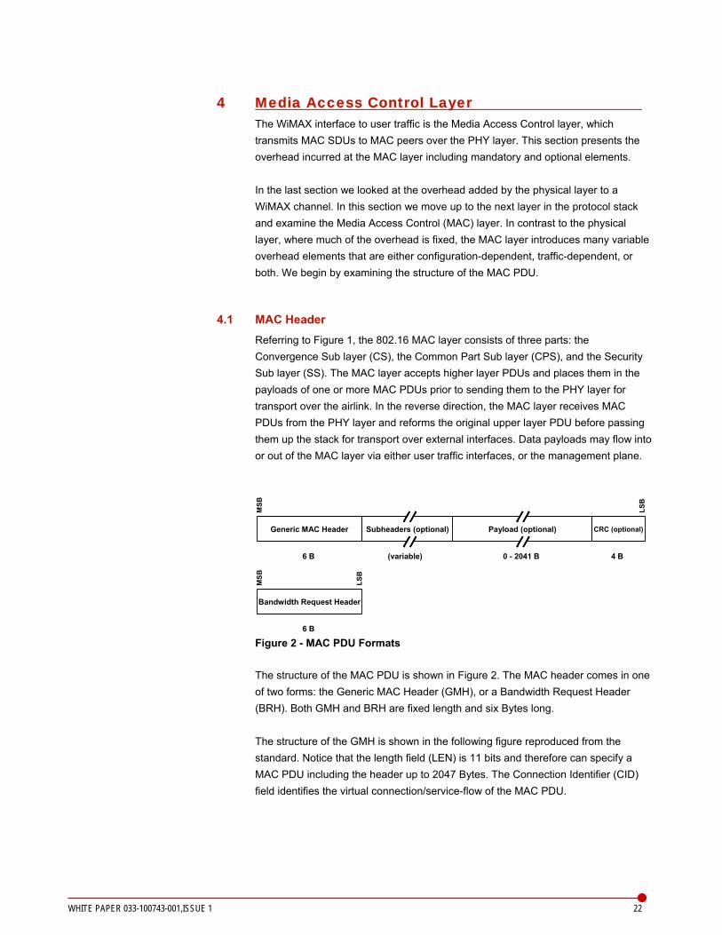
Figure 2 - MAC PDU Formats

he structure of the MAC PDU is shown in Figure 2. The MAC header comes in one

he structure of the GMH is shown in the following figure reproduced from the a

Tof two forms: the Generic MAC Header (GMH), or a Bandwidth Request Header (BRH). Both GMH and BRH are fixed length and six Bytes long. Tstandard. Notice that the length field (LEN) is 11 bits and therefore can specify MAC PDU including the header up to 2047 Bytes. The Connection Identifier (CID)field identifies the virtual connection/service-flow of the MAC PDU.

Generic MAC Header Payload (optional) CRC (optional)

MSB

LSB

Bandwidth Request Header

MSB

LSB

0 - 2041 B 4 B6 B

Subheaders (optional)

(variable)

6 B

Generic MAC Header Payload (optional) CRC (optional)

MSB

LSB

Bandwidth Request Header

MSB

LSB

0 - 2041 B 4 B6 B

Subheaders (optional)

(variable)

6 B


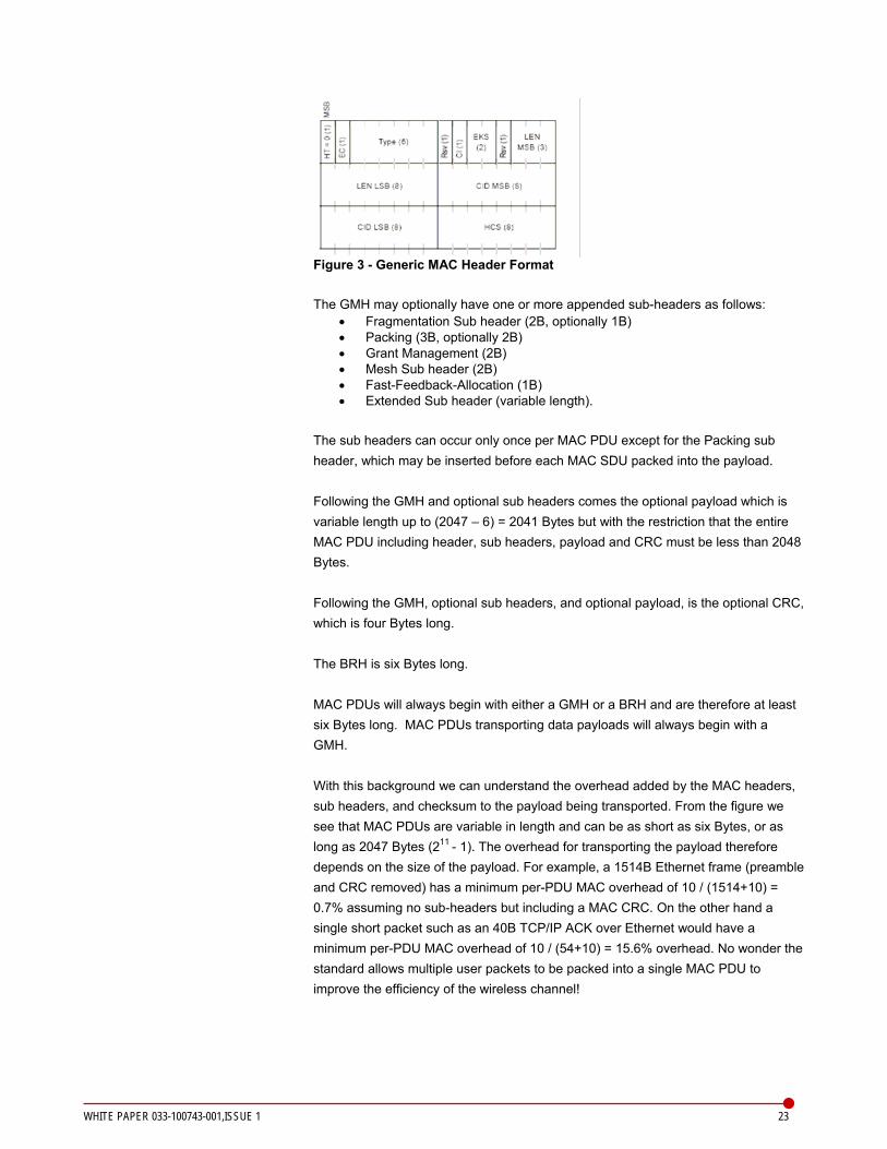
Figure 3 - Generic MAC Header Format The GMH may optionally have one or more appended sub-headers as follows:

• Fragmentation Sub header (2B, optionally 1B) • Packing (3B, optionally 2B) • Grant Management (2B) • Mesh Sub header (2B) • Fast-Feedback-Allocation (1B) • Extended Sub header (variable length).

The sub headers can occur only once per MAC PDU except for the Packing sub header, which may be inserted before each MAC SDU packed into the payload. Following the GMH and optional sub headers comes the optional payload which is variable length up to (2047 – 6) = 2041 Bytes but with the restriction that the entire MAC PDU including header, sub headers, payload and CRC must be less than 2048 Bytes. Following the GMH, optional sub headers, and optional payload, is the optional CRC, which is four Bytes long. The BRH is six Bytes long. MAC PDUs will always begin with either a GMH or a BRH and are therefore at least six Bytes long. MAC PDUs transporting data payloads will always begin with a GMH. With this background we can understand the overhead added by the MAC headers, sub headers, and checksum to the payload being transported. From the figure we see that MAC PDUs are variable in length and can be as short as six Bytes, or as long as 2047 Bytes (211 - 1). The overhead for transporting the payload therefore depends on the size of the payload. For example, a 1514B Ethernet frame (preamble and CRC removed) has a minimum per-PDU MAC overhead of 10 / (1514+10) = 0.7% assuming no sub-headers but including a MAC CRC. On the other hand a single short packet such as an 40B TCP/IP ACK over Ethernet would have a minimum per-PDU MAC overhead of 10 / (54+10) = 15.6% overhead. No wonder the standard allows multiple user packets to be packed into a single MAC PDU to improve the efficiency of the wireless channel!


For analyzing the channel capacity, the 802.16 MAC structure presents some challenges because of the number of optional fields. Each PDU carrying a data payload must have a fixed-size GMH, but what about the optional sub-headers?

4.1.1 Sub headers

Although the additional overhead of the sub headers (typically two Bytes) is small, we should pay attention to it because it potentially affects each MAC PDU that transits the airlink.

4.1.1.1 Fragmentation

Fragmentation refers to splitting a MAC SDU across multiple MAC PDUs.12 The idea is to allow better packing of MAC SDUs into the available OFDM frequency-time resources by using all data sub carriers in each OFDM symbol. Use of fragmentation is optional but encouraged to improve link efficiency. For capacity analysis, it is reasonable to assume that some fraction of the MAC PDUs will be fragmented. The variable overhead is an additional three Bytes added to the 802.16 MAC header for each packed SDU. A worst-case assumption is to assume that each MAC PDU includes a sub header when fragmentation is supported. Both downlink and uplink channels are affected.

4.1.1.2 Packing

Packing refers to combining two or more MAC SDUs into a single MAC PDU. Like its converse, fragmentation, this allows better packing of MAC SDUs into the available OFDM frequency-time resources by using all data sub carriers in each OFDM symbol. Use of packing is optional but encouraged to improve link efficiency. For capacity analysis, it is reasonable to assume that some fraction of the MAC PDUs will be packed. The variable overhead is an additional three Bytes added to the 802.16 MAC header for each packed SDU.13 A worst-case assumption is to assume that each MAC PDU includes a one or more sub headers when packing is supported; the exact number depending on the relative sizes of the SDUs and PDU. Both downlink and uplink channels are affected. Normally packing and fragmentation are either both supported or not at all. Since packing and fragmentation are mutually exclusive operations for a given MAC SDU we can conservatively estimate that, on average, one packing sub header will be present in each MAC PDU increasing the total header overhead by three bytes.

12 The PDUs however must still be part of the same transmission burst and cannot be split across TDMA frames. 13 An exception is made for connections with fixed-length SDUs where a packing sub header is not required.


If packing and fragmentation are not supported then the overhead associated with fractionally used MAUs (see 3.6) will obviously be higher because the scheduler will have fewer options to size the packets to the bandwidth allocations. This will be particularly true for the uplink where only a single station can use a burst. Depending on the traffic characteristics, this increased overhead can often be larger than the small fractional overhead associated with the packing/fragmentation sub headers.

4.1.1.3 Grant Management

The Grant Management (GM) sub header is an optional method for subscriber stations to communicate bandwidth management needs to the base station including poll requests, slip indications, and bandwidth requests. Of these, bandwidth requests are the only form of the sub header of consequence to capacity analysis since they can occur relatively frequently. This method of bandwidth requesting is called a ‘piggyback’ request since it uses an existing uplink MAC PDU to signal the base station that further data remains to be sent. The GM sub header adds two Bytes to the MAC header and only affects the uplink channel overhead. For capacity analysis the worst-case assumption is that each uplink MAC PDU contains a GM sub header. A more realistic assumption is that 10% of the uplink MAC PDUs carry the additional GM sub header overhead.

4.1.1.4 Mesh

The Mesh sub header is intended to support mesh operation where the subscriber stations are allowed to communicate directly without a base station to relay the data. Although the foundations are present in the 802.16 specification, the mesh portion has received comparatively little attention and is relatively immature, reflecting the current market focus on cell coverage deployments with base stations. Accordingly, we will ignore mesh operation in this white paper.

4.1.1.5 Fast-Feedback-Allocation

The Fast-Feedback-Allocation (FFA) sub header is intended as a low-overhead and low-latency method for allocating a small temporary uplink channel for the subscriber station to communicate link information to the base station. It is presently supported only for the OFDMA PHY for mobility and is therefore out of the scope of this white paper.

4.1.1.6 Extended Sub header

The Extended sub header is a new feature added during development of the mobility portion of the 802.16 standard. It supports sleep mode control, sequence number control for handover, and another channel feedback mechanism. Its intended use is mobility support applicable to the OFDMA PHY, and is therefore out of the scope of this white paper.


4.2 Channel Usage Maps The base station controls its sole access to the downlink channel and coordinates multiple access of the uplink to one or more active subscriber stations. Since the downlink is formed by one or more bursts of data, the subscriber stations must have some way of learning the timing of the bursts and whether they need to listen to a given burst to receive their traffic. Similarly, on the uplink the subscriber stations need to have some way of learning when they can transmit on the (sub)channel and for how long. Both of these needs are satisfied in 802.16 by broadcasting channel allocation and usage information in each downlink frame. The information carries no user traffic and is considered part of the downlink channel overhead. We therefore need to take this into account in capacity analysis.

4.2.1 Frame Control Header

Immediately after the downlink preamble (see section 3.4), each downlink frame must have a Frame Control Header (FCH) which is sent at the lowest modulation and coding rate (BPSK 1/2) to ensure all subscriber stations in the coverage cell can receive it. The FCH takes up one MAU, i.e. one OFDM symbol by all data sub carriers. The FCH is used to describe up to four separate broadcast bursts in the downlink frame. Each broadcast burst can use a different modulation and coding profile in order from lowest to highest. The broadcast bursts must begin immediately after the FCH and finish before any other bursts begin. The overhead associated with the FCH is fixed i.e. one MAU each downlink frame. The percentage overhead only changes if the frame length is changed. Examples of data that may be in the first broadcast burst; includes, maps, burst profile descriptions (UCD, DCD), grant allocations for initial ranging, grant allocations for contention bandwidth requests, and so on. Although all subscriber stations listen to the broadcast bursts, there may also be ordinary MAC PDUs with broadcast, multicast, or unicast CIDs sent within a burst.14 It is up to the subscriber station to classify the CIDs in each MAC PDU header to identify traffic destined for it.

4.2.2 Downlink Map

In the first broadcast burst following the FCH, the base station may insert a downlink map to describe other bursts that follow the FCH broadcast burst(s). The size of the downlink map is variable but can be sent with the most efficient modulation and coding acceptable to the intended subscriber station recipients.

14 The waters are a bit murky here. Presumably a subscriber station must listen to all FCH referenced broadcast bursts that it is capable of receiving, i.e. at the modulation and coding it uses and all lower combinations. On the other hand, it is impossible for a subscriber station to decode bursts that are using a higher modulation and coding combination. It is the base station’s responsibility to ensure that all broadcast information, including the maps, DCD, UCD, and so on, are sent in FCH referenced bursts that use the lowest common modulation and coding.


The downlink map begins with eight Bytes of header information followed by one or more information elements (DL-MAP_IE). Each DL-MAP_IE is four Bytes long but can optionally contain variable length extensions. The basic size of the downlink map is therefore 8 + N*4 Bytes, where N is the number of DL-MAP_IE using the frame. There is one information element for each active connection using the downlink frame and the map must terminate with an IE marking the end of the map. A connection is typically associated with one subscriber station (unicast), but can be configured to be shared between multiple stations. The downlink map IE references a specific MAC connection (CID) and a burst profile code (DIUC) so that a subscriber station can know whether a burst contains traffic destined for it or not. This capability allows a subscriber station to skip bursts in the downlink frame that contain no relevant traffic, thus reducing the processing load. Multiple downlink map IE may point to the same burst, so that a burst can be shared between one or more subscriber stations. The subscriber station must therefore be capable of classifying the MAC PDU header CIDs to select the traffic destined for it. How often downlink maps are sent, and therefore the amount of downlink overhead they represent, depends on the channel configuration and how the base station schedules the traffic. In cases where four or fewer burst profiles are in use, the FCH alone could be used to reference all traffic without the need for a downlink map. On the other hand, maps can be used to reduce the amount of downlink processing at the subscriber station at the expense of increased map overhead. Normally this is a design choice made by the base station designers. For worst-case capacity estimation, each downlink frame includes a downlink map whose size is determined by the number of active connections sharing the frame. For example, if there were ten active connections, the size of the basic downlink map would be 8 + 11*4 = 52 Bytes (excluding any extended information elements). How much overhead this takes up in a frame depends on the modulation and coding used to send the map. A worst-case assumption is that there will be some subscriber stations capable of only BPSK modulation and the burst containing the maps will therefore be forced to use this. In our example, a 52 Byte downlink map would occupy five MAUs of the downlink frame using BPSK. Notice that there is a recursive element to the size of the downlink map, set by the number of active stations, which influences the channel capacity, which determines the possible number of active stations! This suggests that accurate capacity analysis needs to iterate to a self-consistent solution.


4.2.3 Uplink Map

Following the FCH and downlink map (if present) the base station may insert an uplink map to indicate how the upcoming uplink channel frame should be allocated. Practically speaking, an uplink map is essential, since without it the subscriber stations would have no way of coordinating their uplink access. The size of the uplink map is variable but can be sent with the most efficient modulation and coding acceptable to the intended subscriber station recipients. The uplink map begins with 11 Bytes of header information followed by one or more information elements (UL-MAP_IE). Each UL-MAP_IE is six Bytes long but can optionally contain variable length extensions. The basic size of the uplink map is therefore 11 + N*6 Bytes, where N is the number of UL-MAP_IE using the frame. There is one information element for each active connection using the frame and the map must terminate with an IE marking the end of the map. Unless contention access is intended, the subscriber station referenced in an UL-MAP_IE by CID must refer to a unique uplink burst since each burst can only be used by a single station. How often uplink maps are sent, and therefore the amount of downlink overhead they represent, depends on the channel configuration and how the base station schedules the traffic. For capacity estimation, each downlink frame includes an uplink map whose size is determined by the number of active connections that will share the uplink frame. For example, if there were ten active connections the size of the basic uplink map would be 11 + 11*6 = 77 Bytes (excluding any extended information elements). Again, how much overhead this takes up in a frame depends on modulation and coding used to send the map. A worst-case assumption is that there will be some subscriber stations capable of receiving only BPSK modulation and the burst containing the maps will therefore be forced to use this. In our example, a 77 Byte uplink map would occupy seven MAUs of the downlink frame using BPSK.

4.2.4 Downlink and Uplink Channel Descriptors

After any downlink and uplink maps in the first broadcast burst the base station may insert a Downlink Channel Descriptor (DCD) and/or an Uplink Channel Descriptor (UCD). The purpose of the DCD/UCD is to define downlink/uplink burst profiles specifying parameters such as modulation type, FEC, scrambler seed, cyclic prefix, and transmit diversity type. Once defined, burst profiles are referred to in later downlink maps via a numerical index called the Downlink Interval Usage Code (DIUC) or Uplink Interval Usage Code (UIUC), which is associated with the profile.


The size of the DCD/UCD is variable depending on the number of downlink/uplink burst profiles elements (Downlink/Uplink_Burst_Profile). Each DCD/UCD begins with three/six bytes of header information followed by one or more channel descriptor information elements. There are many possible options for configuring a channel so the size of the channel descriptor depends on the configuration. For basic licensed FDD operation a DCD/UCD might have 36/32 bytes of channel description and 15/6 bytes for each burst description. There is currently a downlink/uplink limit of 12/8 active burst types at any time but recall that multiple subscriber stations can share a burst profile. How often downlink or uplink channel descriptors are sent, and therefore the amount of downlink overhead they represent, depends on the channel configuration and how often conditions change, thus forcing updates. For example the types of modulation and coding in use could vary over time. In general however the burst profiles will be relatively static and we can ignore them for capacity estimation.

4.3 Bandwidth Requests The 802.16 MAC protocol specifies several different ways that a subscriber station can inform the base station that it has data to send on the uplink. Most of these methods involve sending a BRH (see Figure 2) for which the subscriber station must first obtain an uplink channel access grant from the base station. Since there is overhead associated with getting the grants as well as sending the requests we are interested in the specifics of the bandwidth request mechanism. In this section we will describe the basic mechanisms without explaining why they exist. Later we will see how these are used for providing quality of service (QoS) and further discuss their ramifications on channel overhead in the context of QoS connection profiles.

4.3.1 Contention

Contention based uplink access is a method where the base station periodically allocates part of the uplink channel capacity (grants a “transmit opportunity”) to specified stations that might have data to send. The stations in the contention group are identified by their CID. There are two ways used to manage the process.


4.3.1.1 Full Contention

The mandatory method for issuing the grant is for the base station to include a “REQ Region Full” uplink map information element in the uplink map, which is sent to the subscriber stations on the downlink. There is one information element for each subscriber station CID in the contention group. The information element allocates some whole number of MAU to the stations to use for sending BRH PDUs in the pending uplink frame. Request collisions are handled in the usual exponential back-off fashion so that eventually a station can have its request heard. When the base station receives a BRH it responds by allocating an uplink allocation for the requested CID. A subscriber station that does not see an uplink allocation response from the base station assumes that there has been a collision and retries the request. The overhead associated with this method is in the small addition to the size of uplink map (see 4.2.3), but mainly in the contention allocation itself, which must allow for the most robust modulation and coding combination. The interval between contention allocations is configurable. The uplink contention allocation includes a one-symbol preamble followed by one or more symbols configured for the allocation. The number of symbols depends on the most robust modulation and coding and the number of sub-channels used for the allocation. The size of the allocation should be sufficient to send one BRH. For example, since the BRH is 6 + 4 = 10 Bytes assuming a CRC is used, the number of required symbols is 10 / sizeof(MAU). If there are four sub-channels in the allocation, then from Eq. 10 and Table 1, and assuming BPSK 1/2 modulation and coding, then four OFDM symbols are required to hold one BRH. If desired, the base station can allocate multiple contention allocation opportunities in a frame.

4.3.1.2 Focused Contention

A second optional method for issuing the grant is for the base station to include a “REQ Region Focused” uplink map information element in the uplink map, which is sent to the subscriber stations on the downlink. There is one information element for each subscriber station CID in the contention group. The information element allocates some whole number of OFDM symbols to the stations to use for sending special coded requests for a non-contention bandwidth request allocation in the pending uplink frame. The base station, upon detecting a coded request, sends back an allocation in the uplink map, coupled with its corresponding code index so that subscriber stations can know their request was heard. The subscriber station then uses the non-contention uplink allocation to send a BRH to the base station that responds by granting an uplink allocation for the requested CID in an uplink map. Focused contention is therefore a three-way handshake: subscriber requests a grant, base allocates a grant, and subscriber sends a BRH.15

15 Whether a base station supports Focused Contention is an implementation decision. The mandatory Full Contention method suffers from congestion collapse beyond a ‘knee’ in the curve of the access latency versus number of active subscriber stations. Where this point is varies according to the uplink traffic patterns of the subscriber stations. Focused Contention on the other hand is much more robust and can handle situation where there are a large number of simultaneously contending subscriber stations. The tradeoff is the increased overhead and latency of the three-way handshake.


Request collisions are handled in the usual exponential back-off fashion so that eventually a station can have its request heard. To reduce the chance of collisions Focused Contention subdivides the total uplink data carriers into sub-channel groups of four carriers each and further uses one of eight available CDMA codes for transmitting the request. The codes are transmitted for two consecutive symbols. A subscriber station randomly selects a sub-channel and code index pair. A collision occurs only if two subscriber stations happen to choose the same index pair.16 A subscriber station that does not see an uplink allocation response from the base station assumes that there has been a collision and retries the request. The overhead associated with this method is in the small addition to the size of the uplink map (see 4.2.3), but mainly in the uplink contention allocation itself, plus the following bandwidth request allocation. The interval between contention allocations is configurable. The uplink contention allocation is two OFDM symbols, by all data carriers. This is shared by all requesting stations as explained above. The subsequent uplink bandwidth request allocation, one for each requesting subscriber station, includes a one-symbol preamble followed by one or more symbols configured for the allocation. The number of symbols depends on the modulation and coding and the number of sub-channels used for the allocation. The size of the allocation should be sufficient to send one BRH. For example, since the BRH is 6 + 4 = 10 Bytes, and assuming a CRC is used, then the number of required symbols is 10 / sizeof(MAU). If there are four sub-channels in the allocation, then from Eq. 10 and Table 1, and assuming BPSK 1/2 modulation and coding, four OFDM symbols are required to hold one BRH.

4.3.2 Polling

Polling is a process where the base station periodically allocates part of the uplink channel capacity (issues a “grant” or “transmit opportunity” in the uplink map) to each participating subscriber station that might have data to send. The transmit opportunity itself is the poll, there is no explicit message type. The subscriber stations use the transmit opportunity to send a BRH to request uplink bandwidth. The grants must therefore be at least large enough to send one BRH. Polls may be unicast or multicast or broadcast according to the CID specified in the uplink map transmit opportunity information element. If a poll is multicast or broadcast then one of the contention bandwidth request methods (full or focused) is specified to collect the bandwidth request responses. Unicast polls are directed towards a single CID associated with a single subscriber station. The overhead associated with this method is in the small addition to the size of uplink map (see 4.2.3), but mainly in the request allocation itself, which must allow

16 The odds of choosing the same Focused Contention sub-channel are 1 in 50 and choosing the same code are 1 in 8. The overall collision probability for a given contention opportunity is therefore 1/(50*8) = 0.25%. The tradeoff is the additional complexity, latency, and overhead of the method’s three-way handshake.


for the modulation and coding combination in use by the requesting subscriber station.17 The interval between polls is configurable for a given CID. The uplink contention allocation includes a one-symbol preamble followed by one or more symbols configured for the allocation. The number of symbols depends on the modulation and coding and the number of sub-channels used for the allocation. The size of the allocation should be sufficient to send one BRH. For example, since the BRH is 6 + 4 = 10 Bytes assuming a CRC is used, then the number of required symbols is 10 / sizeof(MAU). If there are four sub-channels in the allocation, then from Eq. 10 and Table 1, assuming BPSK 1/2 modulation and coding, five OFDM symbols by four sub-channels are required to hold one BRH plus the mandatory preamble. For this example, if the polling interval for a connection is configured to be once a frame, and the frame length is 10ms, this amounts to 3B/MAU * 5 MAU / 10ms = 12 kbps in bandwidth request overhead.

4.3.3 Piggyback

A piggyback bandwidth request is a method of using a previously granted uplink channel access opportunity to inform the base station that a subscriber station requires another allocation to send pending data. The idea is that once a subscriber station obtains uplink channel access it can use the channel for future bandwidth requests without incurring the overhead associated with contention or polling. This is most useful when a subscriber station connection has long consecutive trains of data packets to send. To improve efficiency, the method uses a GM sub header of the GMH (see 4.1.1.3). The overhead associated with piggybacking adds two bytes to the length of a MAC PDU. Support for piggyback requests by a subscriber station is optional.

17 In cases where there are a large number of inactive subscriber stations to poll, supporting unicast polling to each of them would be an inefficient use of the downlink frame’s uplink map, and the uplink frame’s bandwidth request opportunities. Multicast polling was designed with this case in mind to improve bandwidth efficiency. The collection of subscriber stations are assigned to a special bandwidth request multicast group and only those that have traffic to send respond to the multicast polls. Broadcast polling is similar, except that all subscriber stations that have traffic to send respond to the polls.


5 Channel Bandwidth Calculation At this point in the white paper it should be readily apparent that there is a complex interrelated array of factors in the WiMAX MAC and PHY layers that influence the channel capacity in terms of the useful available bandwidth. It can be confusing how the various factors should be combined, and in what order, to determine the channel bandwidth capacity. This sections aims to clarify that process. Our approach is to summarize the list of factors in a step-by-step sequence diagram in order to illustrate the process of calculating the useful channel bandwidth. Putting the sequence diagram into practice, we will present an example spreadsheet channel model for exploring various configuration scenarios. In order to keep the discussion to a reasonable length we will focus on a FDD system where the uplink and downlink TDMA frames are independent of one another. Analysis of TDD systems would be similar except user input of the time partitioning of the single uplink/downlink TDMA frame would be required.

input channel size(MHz)

input cyclic prefix(1/4 to 1/32)

calc useful channel bw

input mod and coding distribution

input frame length(2.5 to 20 ms)

calc frame o/h

calc frame bw

calc preamble o/h

calc FCH o/h

calc DL map o/h

calc UL map o/h

calc useful frame bw

calc MAC hdr o/h

calc MAC subhdr o/h

calc MAC CRC o/h

input avg user pk(B)

calc useful MAC bw

1

2

3

4

5

6

7

8

9

10

11

12

13

14

15

16

17






calc frame o/h

calc frame bw

calc preamble o/h

calc FCH o/h

calc DL map o/h

calc UL map o/h


calc MAC hdr o/h

calc MAC subhdr o/h

calc MAC CRC o/h


calc useful MAC bw

1

2

3

4

5

6

7

8

9

10

11

12

13

14

15

16

17

Figure 4 - Downlink Bandwidth Calculation Sequence Beginning with the downlink, Figure 4 presents the sequence diagram for accounting for the various PHY and MAC overhead contributions in order to calculate the useful channel bandwidth. In the figure there are four intermediate results represented in the four columns. In column one the raw channel bandwidth is determined. In column two the basic TDMA framing overhead is accounted for. In column three the required preamble and channel management overhead is taken out. In column four the various per-packet overhead is accounted for resulting finally in the useful user bandwidth available at the input of the MAC protocol layer.


Various user inputs are required to complete the calculation. As indicated in Figure 4, steps 1, 2, 3, 5, 13 call out those inputs which we have already discussed in sections 3 and 4.

calc preamble o/h

calc ranging o/h


calc MAC hdr o/h

calc MAC subhdr o/h

calc MAC CRC o/h


calc useful MAC bw

calc contention o/h

input subch size

input burst size

calc MAU

calc subch o/h






calc frame o/h

calc frame bw

1

2

3

4

5

6

7

8

9

10

11

12

13

14

15

16

17

18

19

20

Figure 5 - Uplink Bandwidth Calculation Sequence Figure 5 presents the companion sequence diagram for the uplink, which similarly accounts for the various PHY and MAC overhead contributions leading to the useful channel bandwidth. As with the downlink there are four intermediate results represented in the four columns. The first two and last columns are identical to the downlink. The third column accounts for the required preambles and required channel management overhead, which differs from downlink. Again, user inputs are required to complete the calculation. These inputs are indicated in steps 1, 2, 3, 5, 9, 12, 16 of Figure 5 as previously discussed in sections 3 and 4.


Figure 6 presents a screen shot of a spreadsheet model which implements the sequence steps of Figure 4 for the downlink and Figure 5 for the uplink on separate tabs (downlink tab shown).18 The cells in blue are the user inputs to the bandwidth calculation. The other cells are formulas or constants that should not be changed. The result of the calculation is shown in the last two rows of the model, which present the aggregate useful channel bandwidth, Cmac, in units of Mbits/s and the equivalent spectral efficiency, Seff, of the channel. By changing the inputs various channel scenarios can be investigated.

Item Value Units Comments

ch_size 3.5 MHz Channel size (sets sampling rate)cyclic_exp 3 # Cyclic prefix exponent N (2 to 5 where 5 represents the shortest prefix), Tg = Tb/2^NBPSK-1/2 5 % Fraction of SS using the modulationQPSK-1/2 2.5 % Fraction of SS using the modulationQPSK-3/4 2.5 % Fraction of SS using the modulation16QAM-1/2 5 % Fraction of SS using the modulation16QAM-3/4 5 % Fraction of SS using the modulation64QAM-2/3 40 % Fraction of SS using the modulation64QAM-3/4 40 % Fraction of SS using the modulationn 1.143 # Sampling factorFs 4.0 MHz Sampling frequencyTb 64.0 us Useful symbol timeTg 8.0 us Guard time (cyclic prefix)Ts 72 us Symbol Time (Tb+Tg)C 9.97 Mbps Useful channel bandwidth

Tf 10 ms Frame length {2.5, 4, 5, 8, 10, 12.5, 20 ms}N 138 symbols Frame length is whole symbolsCf 9.90 Mbps Frame bandwidth

sc 8 subch Configured subch's per SS (1,2,4,8,16), 16 means that SS uses all data subcarriers during uplink accessNfull 1 # / frame Number of Full Contention allocations per frameNfocused 0 # / frame Number of Focused Contention allocations per frame (optional), (set 0 if not supported)NfocusedSS 5 # / frame Number of SS contending with Focused Contention per frameNpolls 5 # / frame Number of bandwidth request polls per frame (one for each polled connection)ranging 3 symbols Initial ranging grant (3 symbols per ranging opportunity)MAU 44.85 Bytes Minimum Allocation Unit (includes average coding and modulation)MAUpf 276 MAU Number of MAU per framefull_cont 2 MAU Full Contention request allocationfocused_cont1 0 symbols Focused Contention request allocation - phase 1focused_cont2 10 MAU Focused Contention request allocation - phase 2p 10 MAU Polling allocationsNb 1 PDU Average number of MAC PDU per burstb 78 Bytes Average burst size (depends on payload size below)b_MAU 3 MAU Average burst allocationbpf 68 # User traffic bursts per frame (ignores fractional filled burst and suboptimal packing efficiency)Cf_useful 5.86 Mbps Useful downlink frame bandwidth

Figure 6 - WiMAX Channel Bandwidth Spreadsheet Model

18 In the Microsoft Word version of this document the spreadsheet is linked as an imbedded object (right-click > worksheet object > open). Otherwise the spreadsheet model file is available on request to SR Telecom.


6 QoS In the previous sections of this white paper we have examined the various factors that influence the overall channel bandwidth. What remains after accounting for the per-channel and per-packet overhead is the usable channel bandwidth. This channel size is the relevant quantity for determining the service capacity consistent with the QoS parameters. The traffic engineering for how the bandwidth is apportioned to the various active connections is typically left to operator configuration. In this section we will illustrate one way in which this could be accomplished. We begin by reviewing the three basic service types supported by WiMAX.

6.1 Constant Bit Rate Services WiMAX compliant systems can support Constant Bit Rate (CBR) by configuring dedicated frequency-time channel grants to specific traffic flows. The dedicated resources correspond to a constant throughput rate. CBR service flows are suitable for applications with strict latency and throughput constraints and that generate a steady stream of fixed size packets such as VoIP. These service flows can be dynamically set up or torn down in response to detection by the system of changing traffic needs. On the downlink, the base station directly controls the scheduling of traffic and allocation of the frequency-time channel resources. Dedicating a portion of the channel bandwidth for CBR flows is therefore a matter of keeping track of the allocated resources and transporting any available packets from appropriately classified traffic. For the uplink the Unsolicited Grant Service (UGS) scheduling method is used. The base station dedicates a portion of the uplink channel bandwidth to a Subscriber Station corresponding to one or more service flows for the duration of the flow. The base station communicates this assignment to the Subscriber Station in the uplink channel usage maps that are periodically broadcast out to all stations. From a capacity standpoint, the key CBR QoS parameter is the unvarying Maximum Sustained Traffic Rate, which is the committed information rate for the flow. The maximum rate is unconditionally dedicated to the flow and therefore can be directly subtracted from the available user channel size to determine the remaining capacity. The only overhead associated with CBR flows is the UGS grant overhead, which increases the size of the uplink channel usage map. Although the bandwidth is dedicated for a CBR service flow, the base station scheduler implementation could still elect to temporarily “borrow” the dedicated bandwidth on the downlink frame if there is no CBR traffic to send. The scheduler must however issue uplink grants according to the CBR service flow configuration whether or not the subscriber station has any traffic to send (the scheduler has no way of knowing in advance).


6.2 Variable Bit Rate Services For applications that have variable traffic throughput demands WiMAX systems support Variable Bit Rate (VBR) services. VBR service flows are suitable for applications that generate fluctuating traffic loads including compressed streaming video and VoIP with silence suppression. On the downlink, the base station directly controls the scheduling of traffic and allocation of the frequency-time channel resources. Dedicating a portion of the channel bandwidth is therefore a matter of keeping track of the allocated resources and transporting any available packets from appropriately classified traffic. The base station performs this scheduling successively for each TDMA frame that is sent out (e.g. every 10 ms) so that the time varying nature of the VBR traffic can be supported in real time. For the uplink there are several scheduling methods depending on the QoS requirements for the service flow. For flows with strict real time access constraints, periodic polling assures that the subscriber station will have guaranteed channel access up to a specified Minimum Reserved Traffic Rate. Real time Polling Service (rtPS) operates by having the base station poll individual subscriber stations periodically (e.g. every frame) to solicit bandwidth requests (see 4.3.2). Extended real time Polling Service (ertPS) operates more like UGS except that the committed maximum rate can be changed on the fly as controlled by subscriber station signaling. For flows with looser real time access constraints, non real time Polling Service (nrtPS) operates like rtPS except the polls can be directed at individual or groups of subscriber stations, and the latency of the base station response to bandwidth requests is not guaranteed.19 The subscriber stations can also use piggyback methods to request continuing channel access (see 4.3.3). For capacity calculations, the two key VBR QoS parameters are the Minimum Reserved Traffic Rate and the Maximum Sustained Traffic Rate. For VBR, the minimum rate corresponds to the committed information rate. Since the minimum rate is guaranteed, it can be directly subtracted from the available user channel size to determine the remaining capacity. The maximum rate is the peak information rate that the system will permit. Traffic, submitted by a subscriber station at rates bounded by the minimum and maximum rates, is dealt with by the base station on a non-guaranteed basis. The overhead associated with VBR service comes from the polling method (see 4.3.2) except for ertPS, which basically has the same overhead as UGS i.e. the size of the uplink channel usage maps is increased for each active flow.

19 If the polls are directed at a group of subscriber stations the responses must use a contention bandwidth request interval to respond since request collisions can occur.


Although the bandwidth is dedicated for the Minimum Reserved portion of the VBR service flow, the base station scheduler implementation could still elect to temporarily “borrow” the dedicated bandwidth on the downlink frame if there is no traffic to send. The scheduler must however issue uplink grants for bandwidth requests according to the VBR service flow configuration for the Minimum Reserved QoS parameter whether or not the subscriber station has any traffic to send (the scheduler has no way of knowing in advance).

6.3 Best Effort Services Best effort (BE) services are intended for service flows with the loosest QoS requirements in terms of channel access latency and without guaranteed bandwidth. Best effort services are appropriate for applications such as web browsing and file transfers that can tolerate intermittent interruptions and reduced throughput without serious consequence. On the downlink, the base station directly controls the scheduling of traffic and allocation of the frequency-time channel resources. For best effort services, the affected traffic is sent as surplus capacity that is available after satisfying other guaranteed service types. On the uplink, the base station should provide periodic contention intervals (see 4.3.1) in order for subscriber stations with best effort flows to submit their bandwidth requests. The subscriber stations can also use piggyback methods to request continuing channel access (see 4.3.3). The overhead associated with best effort services comes from providing the contention intervals for bandwidth requests.

6.4 Sharing Non-Guaranteed Bandwidth In comparing best effort services against variable bit rate services an ambiguity becomes apparent. The system must by definition not admit more guaranteed bandwidth traffic onto the channel than it can supply. On the other hand, VBR and BE services can both have non-guaranteed traffic. For VBR it is the portion of traffic submitted at rates above the Minimum Reserved rate. For BE it is all of the submitted traffic. How should the scheduler deal with this situation in cases where there is insufficient remaining capacity to honor all requests? Shown graphically in Figure 7, what should happen if regions C and D overlap?20 The answer is not specified by the 802.16 standard but is left to vendor implementation.21

20 Note that the figure illustrates the case where the scheduler actually has traffic to fill the guaranteed portion of the channel. If that were not the case then in theory the scheduler can temporarily borrow the guaranteed bandwidth to satisfy non-guaranteed bandwidth requests. For capacity estimations we need to assume the worst case where the guaranteed bandwidth is in use. 21 This should not come as a surprise; the base station scheduler design is similarly not described by the standard. The authors of the standard were trying to balance the conflicting requirements of creating a standard while allowing freedom where possible for product differentiation and innovation.


non-

guar

ante

edgu

aran

teed CBR

VBR

MR

BEVB

RM

S

A

B

C

Dno

n-gu

aran

teed

guar

ante

ed CBR

VBR

MR

BEVB

RM

S

A

B

C

D

Figure 7 – Aggregate Channel Bandwidth Partitioning One simple way to deal with the issue might be to implement a policy of fair-sharing the non-guaranteed bandwidth between VBR and BE. That is, equally divide any remaining bandwidth up between all requesting VBR and BE service flows. The problem with this approach is that is does not allow service providers much control to differentiate their services. The other problem is that, while VBR can specify a minimum information rate, BE services under severe congestion can be starved with throughput rates approaching zero. A better solution is to provide a method for prioritizing access to non-guaranteed bandwidth, which can be done by introducing the concept of service flow over-subscription.22

6.5 Over-Subscription Over-subscription, sometimes called over-booking, in simplest terms means taking advantage of the fact that, for many systems, absolute peak demand on shared resources rarely occur. Examples are everywhere in daily life. Airlines aggressively over-subscribe their seat capacity. Public telephone networks over-subscribe their network switching capacity. The point of over-subscription is that system capacity requirements can be significantly reduced if the requirement to handle absolute worst-case scenarios is ignored. However, over-subscription comes at a price that is related to trading hard guarantees of service for soft statistical guarantees.23 Depending on the nature of shared resource usage (“the traffic”), and how aggressively the resource is over-subscribed, there can be exceptional periods where there is more demand than can be served.

22 The 802.16 standard also includes the ability to specify a traffic priority QoS parameter for VBR and BE service flows. This allows basic grouping of priority between sets of service flows. However, it does not distinguish between guaranteed and non-guaranteed VBR traffic or allow division of priority beyond eight basic levels. 23 How mathematically rigorous the statistics of the guarantees are usually depends on how much is known about the offered traffic. One well-known example is the blocking probability associated with traditional voice Erlang statistics. On the other hand, mixed application packet data networks are notoriously difficult to treat with statistical methods for the general case. Often this results in resorting to empirical rules derived from traffic measurements of a given user population.


In the case of WiMAX networks, operators can choose to over-subscribe the total network capacity in order to improve overall network utilization and cost per line business economics. There are two basic scenarios. An operator can choose to over-subscribe one or more service flow’s ‘guaranteed’ bandwidth, or they might choose to over-subscribe their non-guaranteed bandwidth. Generally over-subscription of guaranteed bandwidth is a practice that operators approach with caution since their customers naturally expect that their service agreements will be honored always. But the fine print of these agreements may also allow for (hopefully) rare periods when the network will not be able to support the guaranteed performance. One simple example could be that VoIP users are guaranteed that less than 1% of their call attempts will be blocked. This can be accomplished by using Erlang statistics to reserve an over-subscribed block of bandwidth sufficient to support a given number of voice lines. Over-subscription of non-guaranteed bandwidth is of course fair game but an operator must still balance their users’ service level expectations against the degree of over-subscription of the network capacity. If users are told that they can expect “up to” some peak level of service but discover that during busy hours that they can only get one tenth of that service they will likely be dissatisfied with their service. Often this is handled by marketing a “typical” level of service associated with a given level of over-subscription (related to the total number of users) and an “up to” service rate limit. Returning to the issue of shared non-guaranteed bandwidth between VBR and BE service flows, one solution for prioritizing the access would be to associate a level of over-subscription to each service flow. For VBR flows there are two relevant independent levels of over-subscription, one for the guaranteed Minimum Reserved portion, and a second for the non-guaranteed portion corresponding to rates bounded by the Minimum Reserved and the Maximum Sustained limits. For BE flows there is just one level of over-subscription associated with the Maximum Sustained limit. If the system allows the service flows to be configured in this manner then the relative priority ranking of the non-guaranteed portions of the VBR and BE service flows can be accomplished. This in turn allows operators to calculate the total number of lines of service that can be provisioned for a given service scenario. In summary of this section, the problem of allocating the aggregate system capacity to the various service flows must take into account the QoS requirements of those flows. Dedicated or guaranteed bandwidth must be dealt with first and what remains is shared by non-guaranteed services. Figure 8 illustrates an example of the allocation sequence. In the figure, steps 8 and 9 are required only if there is more demand for non-guaranteed combined VBR and BE bandwidth than can be served.


calc VBR MS %remaining bw

calc BE MS%remaining bw

alloc VBR MS bwcalc user channel bw

alloc CBR bw

alloc VBR MR bw

calc remaining ch bw


calc VBR MS bw

calc BE MS bw

1

2

3

4

5

6

7

8

9

10

alloc BE MS bw11

no remaining bwdone

12calc VBR MS %remaining bw

calc BE MS%remaining bw

alloc VBR MS bwcalc user channel bw

alloc CBR bw

alloc VBR MR bw



calc VBR MS bw

calc BE MS bw

1

2

3

4

5

6

7

8

9

10

alloc BE MS bw11

no remaining bwdone

12

Figure 8 - Allocating Network Bandwidth


7 Capacity Scenarios We will conclude our discussion of WiMAX capacity by presenting several hypothetical data service and deployment configuration scenarios and analyzing the system capacity

7.1 Broadband Data-Only Operator A intends to deploy a WiMAX based broadband data service to a collection of subscribers and wishes to know how many subscribers each base station channel can support. The operator has determined the following channel parameters:

• 3.5 MHz channels • FDD • 1/8 cyclic prefix • 80% 64QAM (evenly split 3/4, 2/3) • 10% 16QAM (evenly split 3/4, 1/2) • 5% QPSK (evenly split 3/4, 1/2) • 5% BPSK-1/2 • 20 ms frame length • 8 uplink sub-channel allocation groups (2 sub-channels per group) • STC enabled

Using the spreadsheet model calculator in section 5 the usable user downlink channel size is estimated to be 9.3 Mbps. The uplink channel size is estimated to be 5.2 Mbps. Because the expected downlink/uplink offered traffic ratio is expected to be 4:1, whereas the channel bandwidth ratio is about 2:1, the system will be constrained by downlink bandwidth and the capacity analysis can ignore the uplink. The operator has determined the following downlink service parameters:

• ‘Platinum’ subscribers: VBR, 1 Mbps minimum reserved (OSR 10), 3 Mbps maximum sustained (OSR 20), SME users, 5% of total subscriber population

• ‘Gold’ subscribers: VBR, 500 Mbps minimum reserved (OSR 10), 1 Mbps maximum sustained (OSR 20), SOHO users, 10% of total subscriber population

• ‘Silver’ subscribers: BE, 1 Mbps maximum sustained (OSR 20), residential users, 85% of total subscriber population

To determine the channel capacity in terms of the number of subscribers we need to determine the average bandwidth for each type of subscriber weighted by the take rate for that type:

<BW> = 5%*[1000/10+(3000-1000)/20] + 10%[500/10+(1000-500)/20] + 85%*[1000/20] <BW> = 60 kbps/sub.


The estimated capacity of the channel is therefore:

Nsub = 9.3 Mbps / 60 kbps/sub = 155 subscribers. The operator can use this information to help determine the required number of channels (sectors) per base station and where the base stations should be located.

7.2 Mixed Voice and Broadband Operator B plans to offer combined VoIP voice and broadband data services and wishes to know how many subscribers each base station channel can support. The operator has determined the following channel parameters (same as above except shorter frame time to reduce VoIP latency):

• (same as above) • 10 ms frame length

Using the spreadsheet model calculator in section 5 the usable user downlink channel size is estimated to be 8.8 Mbps. The uplink channel size is estimated to be 4.8 Mbps. The expected broadband downlink/uplink offered traffic ratio is expected to be 4:1. The voice downlink/uplink offered traffic ration is expected to be 1:1. It is unclear whether the uplink or downlink channel will constrain the capacity so both are considered in the analysis. The operator has determined the following downlink service parameters:

• ‘Platinum’ subscribers: VBR, 1 Mbps minimum reserved (OSR 10), 3 Mbps maximum sustained (OSR 20), SME users, 5% of total subscriber population

• ‘Gold’ subscribers: VBR, 500 Mbps minimum reserved (OSR 10), 1 Mbps maximum sustained (OSR 20), SOHO users, 10% of total subscriber population

• ‘Silver’ subscribers: BE, 1 Mbps maximum sustained (OSR 20), residential users, 85% of total subscriber population

• VoIP subscribers: CBR, 100mE/line, 1% GoS, 100% of total subscriber population, G.711 vocoder with compressed RTP headers and UDP checksums.

The operator has determined the following uplink service parameters:

• Broadband data (same as downlink except all rates reduced by 1/4) • VoIP subscribers: (same as downlink).

Neglecting VoIP for the moment, the average downlink data rate per subscriber is:

<BW> = 5%*[1000/10+(3000-1000)/20] + 10%[500/10+(1000-500)/20] + 85%*[1000/20] <BW> = 60 kbps/sub.


The same calculation for the average uplink data rate per subscriber is:

<BW> = 5%*[250/10+(750-250)/20] + 10%[125/10+(250-125)/20] + 85%*[250/20] <BW> = 15 kbps/sub. To account for the VoIP traffic we should consider the vocoder data rate and Erlang statistics. For G.711, with cRTP and UDP checksums, the operator determines that the rate is about 82 kbps counting all application header overhead (except 802.16). In order to know the amount of bandwidth that must be reserved for the peak number of simultaneous calls, the total number of lines must be known. Unfortunately, that is precisely what the operator is trying to determine so the operator “guesses” that the system can support 120 total lines. The estimated total offered traffic will then be:

T = 120 lines * 100mE/line = 12.0 Erlang Assuming 1% GoS this equates (using ErlangB tables) to as many as 20 simultaneous calls. The total bandwidth required to support VoIP will therefore be:

BWvoip = 20 * 82 kbps = 1640 kbps. The VoIP dedicated bandwidth needs to be deducted from the available channel before calculating the total broadband data subscriber capacity.

Nsub = (8.8 Mbps – 1.6 Mbps) / 60 kbps/sub = 120 subscribers.24

Now we need to check the capacity of the uplink:

Nsub = (4.8 Mbps – 1.6 Mbps) / 15 kbps/sub = 213 subscribers. Once again the constraining channel is the downlink and the capacity is therefore 120 voice and broadband data subscribers per channel. The operator can use this information to help determine the required number of channels (sectors) per base station and where the base stations should be located.

24 Obviously the operator’s “guess” of the correct number of lines was fortuitous for purposes of illustration. In general the answer can be obtained by successively iterating to a self-consistent answer.


8 Summary In this white paper we have attempted to show why access and service providers need to have detailed knowledge of their WiMAX system’s capacity in order to successfully deploy their intended services. One of WiMAX’s advantages is the high degree of configurability, which translates to being adaptable to diverse service scenarios. Analysis of WiMAX capacity therefore depends on many interrelated channel configuration options and protocol overhead considerations. It is this very flexibility that makes it difficult to generalize about the system capacity. We have presented a thorough discussion of the various contributions to the system overhead from the MAC and PHY layers. To illustrate the procedure of calculating the bandwidth capacity we discussed the analysis sequence flow and presented a spreadsheet model of the bandwidth capacity. With an understanding of system bandwidth capacity in hand, we discussed the WiMAX QoS model and the partitioning of the available bandwidth into the three basic service types. Finally, we looked at two hypothetical WiMAX service scenarios, using the tools developed in this white paper to arrive at a capacity in terms of the number of users that could be supported.


Corporate Headquarters 8150 Trans-Canada Hwy.

Montreal, QC H4S 1M5

Canada [email protected] www.srtelecom.com

wimax capacity white paper - pudn.comread.pudn.com/downloads167/doc/766153/wimax-capacity_3.pdf ·...

Documents