. . . . . . . . . .

Wind Diversity Enhancement of Wyoming/Colorado Wind Energy Projects The Second in a series of four studies on geographic diversity

Jonathan Naughton, Thomas Parish, and Jerad Baker Final Report Submitted to the Wyoming Infrastructure Authority

April 2013

Wind Energy Research Center (WERC) College of Engineering and Applied Science Dept. 3295, 1000 E. University Ave. Laramie, WY 82070 Phone: (307)766-6284 Fax: (307)766-2695

The authors of this study would like to acknowledge the financial support provided by the Wyoming Infrastructure Authority. In addition, the support provided by Loyd Drain, Executive Director of the Wyoming Infrastructure Authority is gratefully acknowledged. This document is copyrighted by the University of Wyoming, all rights reserved. © 2013 The U.S. Department of Energy and the State of Wyoming are granted a royalty-free, non-exclusive, unlimited and irrevocable license to reproduce, publish, or other use of this document. Such parties have the authority to authorize others to use this document for federal and state government purposes. Any other redistribution or reproduction of part or all of the contents in any form is prohibited other than for your personal and non-commercial use. Any reproduction by third parties must include acknowledgement of the ownership of this material. You may not, except with our express written permission, distribute or commercially exploit the content. Nor may you transmit it or store it in any other website or other form of electronic retrieval system. This report is the second in a series of four reports to compare the geographic diversity of Wyoming wind with wind resources

1. in California (released January 25, 2013); 2. in Colorado; 3. in Nebraska; and 4. within Wyoming.

2

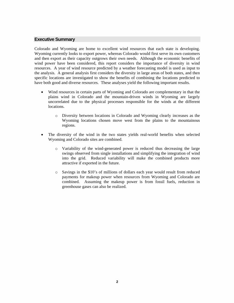
Executive Summary

Colorado and Wyoming are home to excellent wind resources that each state is developing. Wyoming currently looks to export power, whereas Colorado would first serve its own customers and then export as their capacity outgrows their own needs. Although the economic benefits of wind power have been considered, this report considers the importance of diversity in wind resources. A year of wind resource predicted by a weather forecasting model is used as input to the analysis. A general analysis first considers the diversity in large areas of both states, and then specific locations are investigated to show the benefits of combining the locations predicted to have both good and diverse resources. These analyses yield the following important results.

Wind resources in certain parts of Wyoming and Colorado are complementary in that the plains wind in Colorado and the mountain-driven winds in Wyoming are largely uncorrelated due to the physical processes responsible for the winds at the different locations.

o Diversity between locations in Colorado and Wyoming clearly increases as the Wyoming locations chosen move west from the plains to the mountainous regions.

The diversity of the wind in the two states yields real-world benefits when selected Wyoming and Colorado sites are combined.

o Variability of the wind-generated power is reduced thus decreasing the large swings observed from single installations and simplifying the integration of wind into the grid. Reduced variability will make the combined products more attractive if exported in the future.

o Savings in the $10’s of millions of dollars each year would result from reduced payments for makeup power when resources from Wyoming and Colorado are combined. Assuming the makeup power is from fossil fuels, reduction in greenhouse gases can also be realized.

3

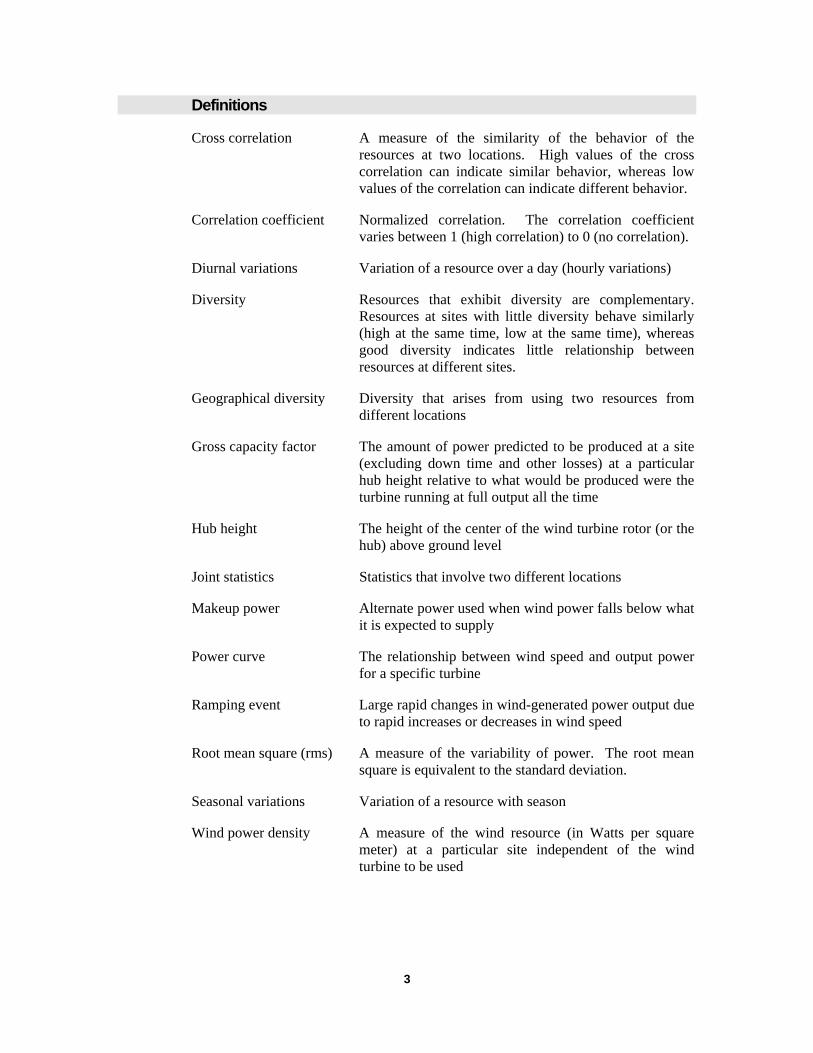
Definitions

Cross correlation A measure of the similarity of the behavior of the resources at two locations. High values of the cross correlation can indicate similar behavior, whereas low values of the correlation can indicate different behavior.

Correlation coefficient Normalized correlation. The correlation coefficient varies between 1 (high correlation) to 0 (no correlation).

Diurnal variations Variation of a resource over a day (hourly variations)

Diversity Resources that exhibit diversity are complementary. Resources at sites with little diversity behave similarly (high at the same time, low at the same time), whereas good diversity indicates little relationship between resources at different sites.

Geographical diversity Diversity that arises from using two resources from different locations

Gross capacity factor The amount of power predicted to be produced at a site (excluding down time and other losses) at a particular hub height relative to what would be produced were the turbine running at full output all the time

Hub height The height of the center of the wind turbine rotor (or the hub) above ground level

Joint statistics Statistics that involve two different locations

Makeup power Alternate power used when wind power falls below what it is expected to supply

Power curve The relationship between wind speed and output power for a specific turbine

Ramping event Large rapid changes in wind-generated power output due to rapid increases or decreases in wind speed

Root mean square (rms) A measure of the variability of power. The root mean square is equivalent to the standard deviation.

Seasonal variations Variation of a resource with season

Wind power density A measure of the wind resource (in Watts per square meter) at a particular site independent of the wind turbine to be used

4

Introduction

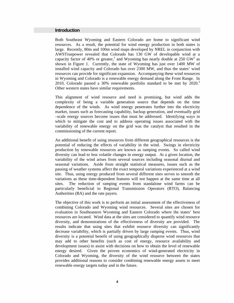
Both Southeast Wyoming and Eastern Colorado are home to significant wind resources. As a result, the potential for wind energy production in both states is large. Recently, 80m and 100m wind maps developed by NREL in conjunction with AWSTruepower revealed that Colorado has 130 GW of developable wind at a capacity factor of 40% or greater,1 and Wyoming has nearly double at 250 GW2 as shown in Figure 1. Currently, the state of Wyoming has just over 1400 MW of installed wind capacity and Colorado has over 2300 MW, and thus the states’ wind resources can provide for significant expansion. Accompanying these wind resources in Wyoming and Colorado is a renewable energy demand along the Front Range. In 2010, Colorado passed a 30% renewable portfolio standard to be met by 2020.3 Other western states have similar requirements.

This alignment of wind resource and need is promising, but wind adds the complexity of being a variable generation source that depends on the time dependence of the winds. As wind energy penetrates further into the electricity market, issues such as forecasting capability, backup generation, and eventually grid –scale energy sources become issues that must be addressed. Identifying ways in which to mitigate the cost and to address operating issues associated with the variability of renewable energy on the grid was the catalyst that resulted in the commissioning of the current report.

An additional benefit of using resources from different geographical resources is the potential of reducing the effects of variability in the wind. Swings in electricity production by renewable resources are known as ramping events. So called wind diversity can lead to less volatile changes in energy output. At a given location, the variability of the wind arises from several sources including seasonal diurnal and seasonal variations. Aside from straight statistical measures, issues such as the passing of weather systems affect the exact temporal variations experienced at a wind site. Thus, using energy produced from several different sites serves to smooth the variations as these time-dependent features will not happen at the same time at all sites. The reduction of ramping events from standalone wind farms can be particularly beneficial to Regional Transmission Operators (RTO), Balancing Authorities (BA) and the rate payers.

The objective of this work is to perform an initial assessment of the effectiveness of combining Colorado and Wyoming wind resources. Several sites are chosen for evaluation in Southeastern Wyoming and Eastern Colorado where the states’ best resources are located. Wind data at the sites are considered to quantify wind resource diversity, and demonstrations of the effectiveness of diversity are provided. The results indicate that using sites that exhibit resource diversity can significantly decrease variability, which is partially driven by large ramping events. Thus, wind diversity is a potential benefit of using geographically disperse wind resources that may add to other benefits (such as cost of energy, resource availability and development issues) to assist with decisions on how to obtain the level of renewable energy desired. Given the proven economics of wind-generated electricity in Colorado and Wyoming, the diversity of the wind resource between the states provides additional reasons to consider combining renewable energy assets to meet renewable energy targets today and in the future.

5

Figure 1 – Wind development potential in Colorado and Wyoming at various gross capacity factors. A hub height of 80 m has been assumed. This figure has been adapted from references 1 and 2.

Description of Wyoming and Colorado Winds

Wyoming and Colorado winds are quite different due to different factors that influence them. Southeast Wyoming winds are driven by the topography, elevation, and the weather conditions that result. Flow through the low point in the continental divide caused by pressure differences that set up across Wyoming in the winter cause that season to have the best wind resource. However, wind resource remains very good throughout the rest of the year, with a fairly significant decrease in winds in the late summer. See a companion report on Wyoming wind diversity for a more detailed discussion of Wyoming’s wind.4

The Eastern Plains of Colorado are characterized by strong dry winds in the winter, but high winds can extend into the spring in many places. Approaching the Mountains from the East, the winds become lighter but are subject to Chinook and Bora winds due to the mountains.5

As is evident, the processes affecting the winds in Wyoming and Colorado are significantly different, which should provide beneficial diversification should wind plants at multiple sites be used to provide power for the Front Range.

Approach

Overview To investigate the promise of wind diversity on wind energy power production, an initial investigation using data from a mesoscale weather forecasting model is carried out. One year of data for multiple sites in Wyoming and Colorado is used. Monthly average wind speeds are investigated to characterize overall trends, whereas correlations between sites are used to estimate diversity. Finally, power production from a distribution of turbines over different combination of sites is determined.

30 40 50 600

200

400

600

800

GCF - Gross Capacity Factor (%)

Pow

er C

apac

ity

abov

e G

CF

(GW

)

Wyoming

Colorado

6

While not comprehensive in nature, these analyses clearly support the potential importance of wind diversification.

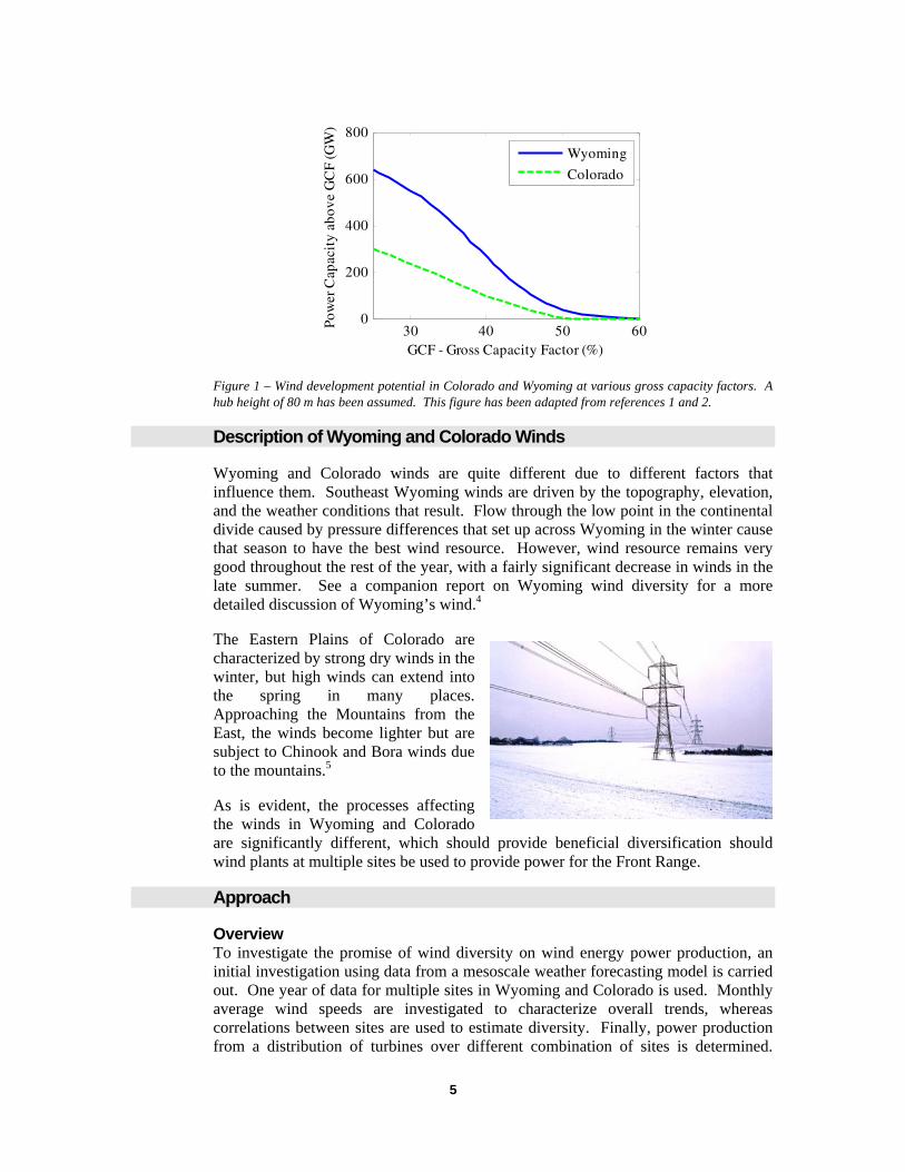
Locations Chosen For this initial study, five locations in the wind producing areas in Southeastern Wyoming were selected for the analysis: sites near Rawlins (RSW), Casper (CNE), Medicine Bow (MBW), Southern Laramie Valley (LVS), and Wheatland/Chugwater (WC). These areas, shown in Figure 2 are near current wind plants or those that have been proposed for development. In Colorado, the locations of five existing installations were chosen to cover the range of conditions expected in this region: Cedar Creek (CC), Peetz Table (PT), Cedar Point (CP), Kit Carson (KC), and Colorado Green (CG). These locations are also shown in Figure 2.

Figure 2- Ten wind sites selected for the Wyoming/Colorado wind diversity study.

Description of Data Sets The data used for these studies was obtained from the Weather Research Forecast Model (WRF) run with a High Resolution Window (HRW) that provides 4 km horizontal spacing. The closest grid point in these data sets to the points identified in Figure 2 was used to provide wind information. The data used here were extracted from one of four WRF runs performed each day, and data were taken from the model for 24 hours past the start time. The next day’s simulations were then used to continue the data from that point. One year of data was used starting in July 1, 2009 extending until June 30, 2010. For some periods of heavy forecasting use (e.g. the month of August), the solutions did not exist due to the need to use computational resources for other purposes (e.g. Hurricane modeling). Data extracted from the model were used to estimate hourly wind speeds at 80 m above the ground.

Analysis Performed Several types of analysis were performed here to evaluate wind diversity. First the annual wind power densities (the average of the instantaneous wind power density

1/2 , where is the density and is the instantaneous velocity at the height

Wyoming

Colorado

WC

CNE

RSW

LVS

MBW

CC PT

CP KC

CG

7

of interest) at 80 m above ground level were determined to locate likely sites for development and to provide an evaluation of the wind resource at locations of existing wind sites. Next, correlations were performed between specific sites in one state with sites in the region of interest in the other state. Using site pairs with promising correlations, monthly and diurnal wind speeds and power production estimates were all used to demonstrate the benefits of diversity. Determination of correlations and power production is discussed in more detail below.

Joint statistics between sites are the primary means used to quantify diversity. For this

purpose, scatter plots of the wind power density at two locations were first considered. Such plots graphically depict the relationship between the winds at different times. To quantity this relationship, the cross correlation of the wind power density between the two sites was calculated using

∑ ,

and the corresponding cross correlation coefficient was defined here as

/ / ,

where p1 and p2 are the wind power density at the different sites identified by x1 and x2, and N is the number of wind power densities that are used in the determination of R. The first equation is equivalent to the cross-correlation function at zero time lag as defined in reference 6. When the correlation coefficient is one, the winds at the two locations follow each other exactly (perfectly correlated). When the correlation coefficient is zero, the winds at the two sites are uncorrelated, which is the desired case for wind diversity.

To demonstrate the beneficial effects of choosing sites with diverse wind, the combined power production of different sites was considered. The time history of production was considered as were the mean and variance of the power production for the year. The production was determined by choosing a wind turbine power curve (here the GE 1.5 XLE) and using the hourly wind data to determine instantaneous power. This instantaneous power was then integrated over time to determine energy production ,

∑ ∆ ,

where is the wind turbine power at velocity , and ∆ is the time between velocity samples (1 hour in this case), and N is the number of velocity samples used to determine E. The average power could then be determined using

/ ∑ ∆ .

8

Results

The analysis processes described above were applied to wind data from Wyoming and Colorado to assess the benefits of diversity. The wind power density determined from the data is first described followed by a discussion of the correlation results. Finally, evidence of the benefits of diversity are shown by choosing promising locations from the correlation results and determining the winds and resulting power produced at those sites.

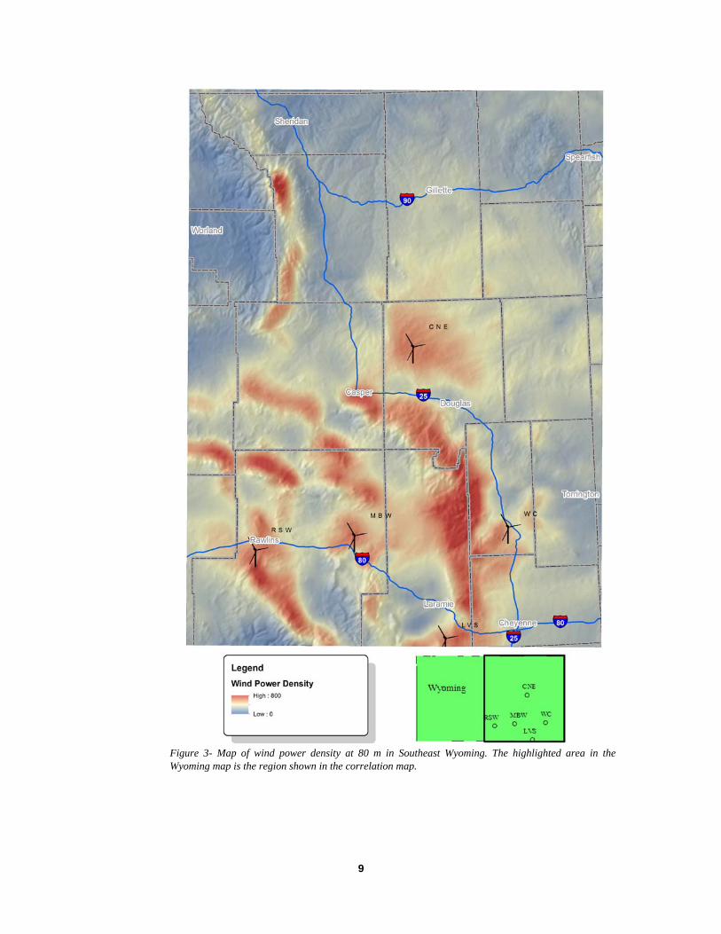
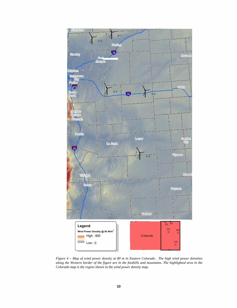
Wind Power Density Prior to performing correlations, it is important to ensure that the points used for the correlations are favorable sites for wind power production. The wind power density at 80 meters above ground provides a measure of the wind potential and is shown for Eastern Wyoming in Figure 3 and for Eastern Colorado in Figure 4. Regions with wind power densities above 400 W/m2 (pink) are considered likely to be good sites, whereas higher wind power densities (reds) would be considered to be excellent. Also shown in the figure are the sites chosen for analysis. It is clear in these figures that high quality wind resource is widespread in Southeast Wyoming, whereas lower, but still respectable, wind power densities exist in Eastern Colorado. All the sites in Southeast Wyoming chosen for further study are in regions of high quality wind (wind power density > 500 W/m2), whereas the sites chosen in Colorado are near current wind farms and represent areas of good wind resource. Having ensured the quality of the wind at these locations, correlation analysis was undertaken.

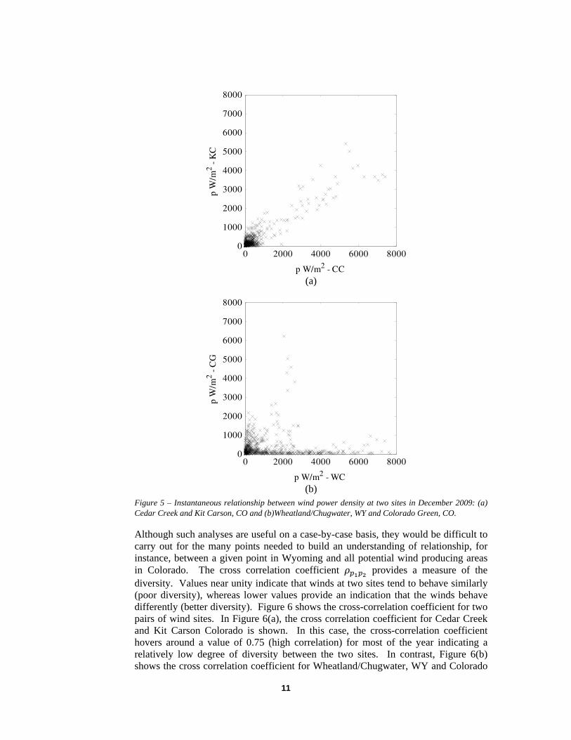
Correlations The average wind power density provides an indication of good wind resource locations, but it does not provide any information about the potential diversity of two sites. To understand the concept of diversity and its relationship to correlations, consider Figure 5 that shows the instantaneous wind power densities at two pairs of locations for one month. The wind power densities at Cedar Creek, CO and Kit Carson, CO, shown in Figure 5 (a), lie along a line from the bottom left hand to the top right hand of the figure indicating that the winds tend to be similar at the same time, or are highly correlated and exhibit little diversity. In contrast, Figure 5 (b) shows a much different result for Wheatland/Chugwater, WY and Colorado Green, CO. In this case, the points are much more scattered and often lie along the horizontal or vertical axes. This result suggests that the winds at the two sites are uncorrelated and exhibit good diversity.

9

Figure 3- Map of wind power density at 80 m in Southeast Wyoming. The highlighted area in the Wyoming map is the region shown in the correlation map.

10

Figure 4 – Map of wind power density at 80 m in Eastern Colorado. The high wind power densities along the Western border of the figure are in the foothills and mountains. The highlighted area in the Colorado map is the region shown in the wind power density map.

11

(a)

(b)

Figure 5 – Instantaneous relationship between wind power density at two sites in December 2009: (a) Cedar Creek and Kit Carson, CO and (b)Wheatland/Chugwater, WY and Colorado Green, CO.

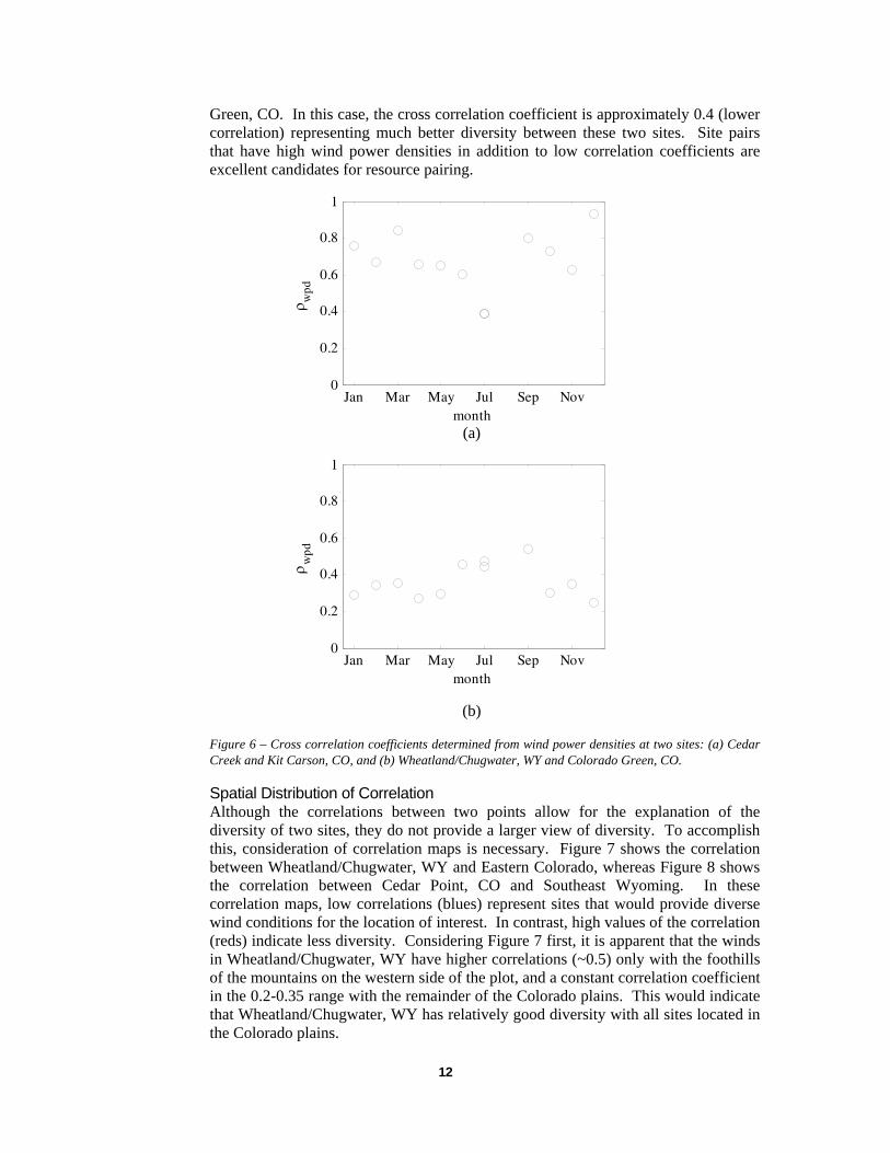
Although such analyses are useful on a case-by-case basis, they would be difficult to carry out for the many points needed to build an understanding of relationship, for instance, between a given point in Wyoming and all potential wind producing areas in Colorado. The cross correlation coefficient provides a measure of the diversity. Values near unity indicate that winds at two sites tend to behave similarly (poor diversity), whereas lower values provide an indication that the winds behave differently (better diversity). Figure 6 shows the cross-correlation coefficient for two pairs of wind sites. In Figure 6(a), the cross correlation coefficient for Cedar Creek and Kit Carson Colorado is shown. In this case, the cross-correlation coefficient hovers around a value of 0.75 (high correlation) for most of the year indicating a relatively low degree of diversity between the two sites. In contrast, Figure 6(b) shows the cross correlation coefficient for Wheatland/Chugwater, WY and Colorado

0 2000 4000 6000 80000

1000

2000

3000

4000

5000

6000

7000

8000

p W/m2 - CC

p W

/m2 -

KC

0 2000 4000 6000 80000

1000

2000

3000

4000

5000

6000

7000

8000

p W/m2 - WC

p W

/m2 -

CG

12

Green, CO. In this case, the cross correlation coefficient is approximately 0.4 (lower correlation) representing much better diversity between these two sites. Site pairs that have high wind power densities in addition to low correlation coefficients are excellent candidates for resource pairing.

(a)

(b)

Figure 6 – Cross correlation coefficients determined from wind power densities at two sites: (a) Cedar Creek and Kit Carson, CO, and (b) Wheatland/Chugwater, WY and Colorado Green, CO.

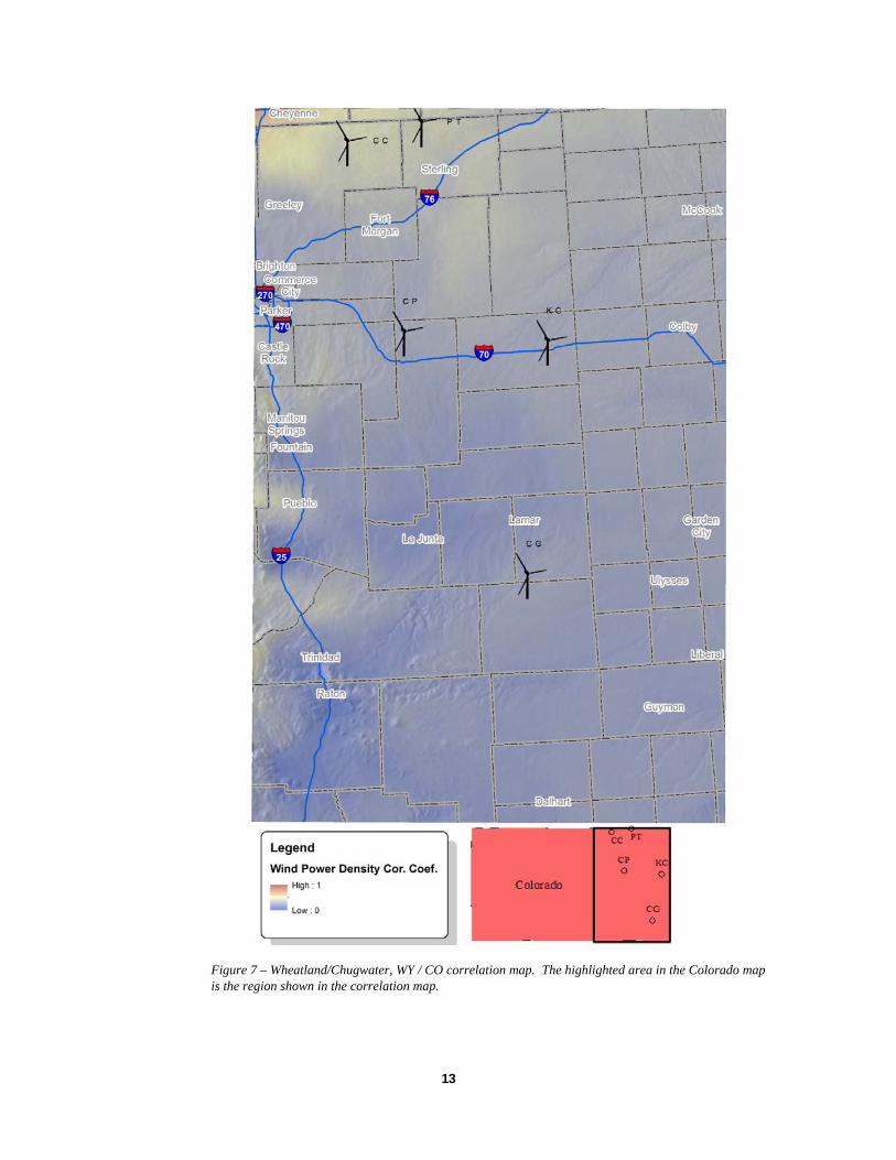
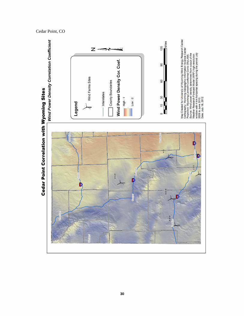
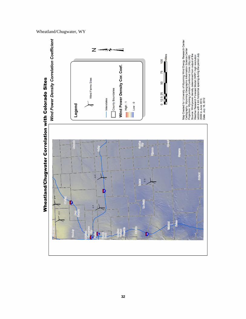
Spatial Distribution of Correlation Although the correlations between two points allow for the explanation of the diversity of two sites, they do not provide a larger view of diversity. To accomplish this, consideration of correlation maps is necessary. Figure 7 shows the correlation between Wheatland/Chugwater, WY and Eastern Colorado, whereas Figure 8 shows the correlation between Cedar Point, CO and Southeast Wyoming. In these correlation maps, low correlations (blues) represent sites that would provide diverse wind conditions for the location of interest. In contrast, high values of the correlation (reds) indicate less diversity. Considering Figure 7 first, it is apparent that the winds in Wheatland/Chugwater, WY have higher correlations (~0.5) only with the foothills of the mountains on the western side of the plot, and a constant correlation coefficient in the 0.2-0.35 range with the remainder of the Colorado plains. This would indicate that Wheatland/Chugwater, WY has relatively good diversity with all sites located in the Colorado plains.

Jan Mar May Jul Sep Nov0

0.2

0.4

0.6

0.8

1

month

wpd

Jan Mar May Jul Sep Nov0

0.2

0.4

0.6

0.8

1

month

wpd

13

Figure 7 – Wheatland/Chugwater, WY / CO correlation map. The highlighted area in the Colorado map is the region shown in the correlation map.

14

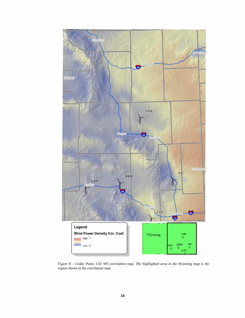
Figure 8 – Cedar Point, CO/ WY correlation map. The highlighted area in the Wyoming map is the region shown in the correlation map.

15

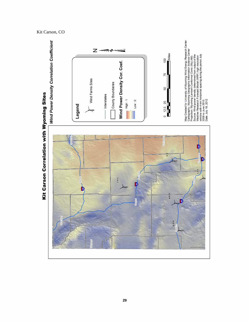
In contrast, Figure 8 indicates that Cedar Point, CO is more highly correlated with the eastern part of the portion of Wyoming shown, with cross correlation coefficients at the 0.8 level. The region of high correlation in the figure is on the plains well east of the mountains and exhibits wind characteristics of the plains much like those found in Colorado. At locations further west, the cross correlation rapidly drops as the wind characteristics change. Maps such as those in Figure 7 and Figure 8 clearly show where wind farms should be paired to maximize diversity. Additional correlation maps for all the sites considered in this study are provided in Appendix 1 – Wind Correlation Maps.

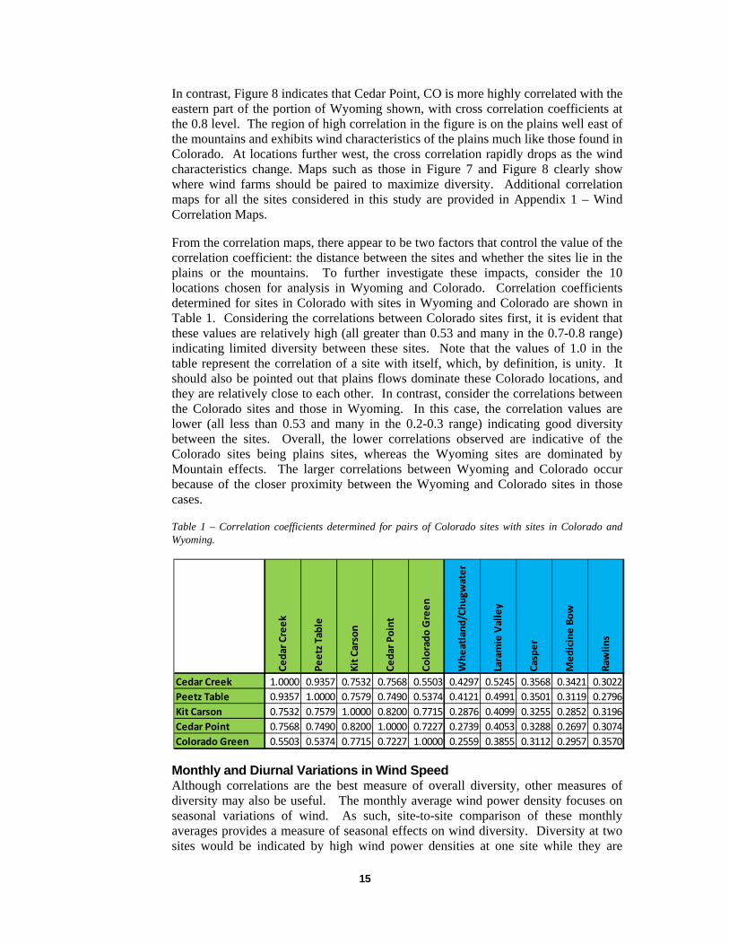
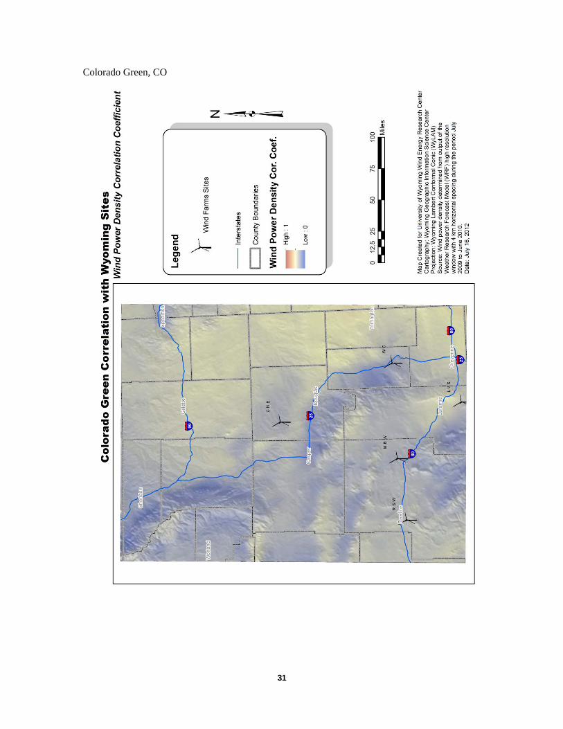
From the correlation maps, there appear to be two factors that control the value of the correlation coefficient: the distance between the sites and whether the sites lie in the plains or the mountains. To further investigate these impacts, consider the 10 locations chosen for analysis in Wyoming and Colorado. Correlation coefficients determined for sites in Colorado with sites in Wyoming and Colorado are shown in Table 1. Considering the correlations between Colorado sites first, it is evident that these values are relatively high (all greater than 0.53 and many in the 0.7-0.8 range) indicating limited diversity between these sites. Note that the values of 1.0 in the table represent the correlation of a site with itself, which, by definition, is unity. It should also be pointed out that plains flows dominate these Colorado locations, and they are relatively close to each other. In contrast, consider the correlations between the Colorado sites and those in Wyoming. In this case, the correlation values are lower (all less than 0.53 and many in the 0.2-0.3 range) indicating good diversity between the sites. Overall, the lower correlations observed are indicative of the Colorado sites being plains sites, whereas the Wyoming sites are dominated by Mountain effects. The larger correlations between Wyoming and Colorado occur because of the closer proximity between the Wyoming and Colorado sites in those cases.

Table 1 – Correlation coefficients determined for pairs of Colorado sites with sites in Colorado and Wyoming.

Monthly and Diurnal Variations in Wind Speed Although correlations are the best measure of overall diversity, other measures of diversity may also be useful. The monthly average wind power density focuses on seasonal variations of wind. As such, site-to-site comparison of these monthly averages provides a measure of seasonal effects on wind diversity. Diversity at two sites would be indicated by high wind power densities at one site while they are

Cedar Creek

Peetz Table

Kit Carson

Cedar Point

Colorado Green

Wheatland/Chugw

ater

Laramie Valley

Casper

Medicine Bow

Raw

lins

Cedar Creek 1.0000 0.9357 0.7532 0.7568 0.5503 0.4297 0.5245 0.3568 0.3421 0.3022

Peetz Table 0.9357 1.0000 0.7579 0.7490 0.5374 0.4121 0.4991 0.3501 0.3119 0.2796

Kit Carson 0.7532 0.7579 1.0000 0.8200 0.7715 0.2876 0.4099 0.3255 0.2852 0.3196

Cedar Point 0.7568 0.7490 0.8200 1.0000 0.7227 0.2739 0.4053 0.3288 0.2697 0.3074

Colorado Green 0.5503 0.5374 0.7715 0.7227 1.0000 0.2559 0.3855 0.3112 0.2957 0.3570

16

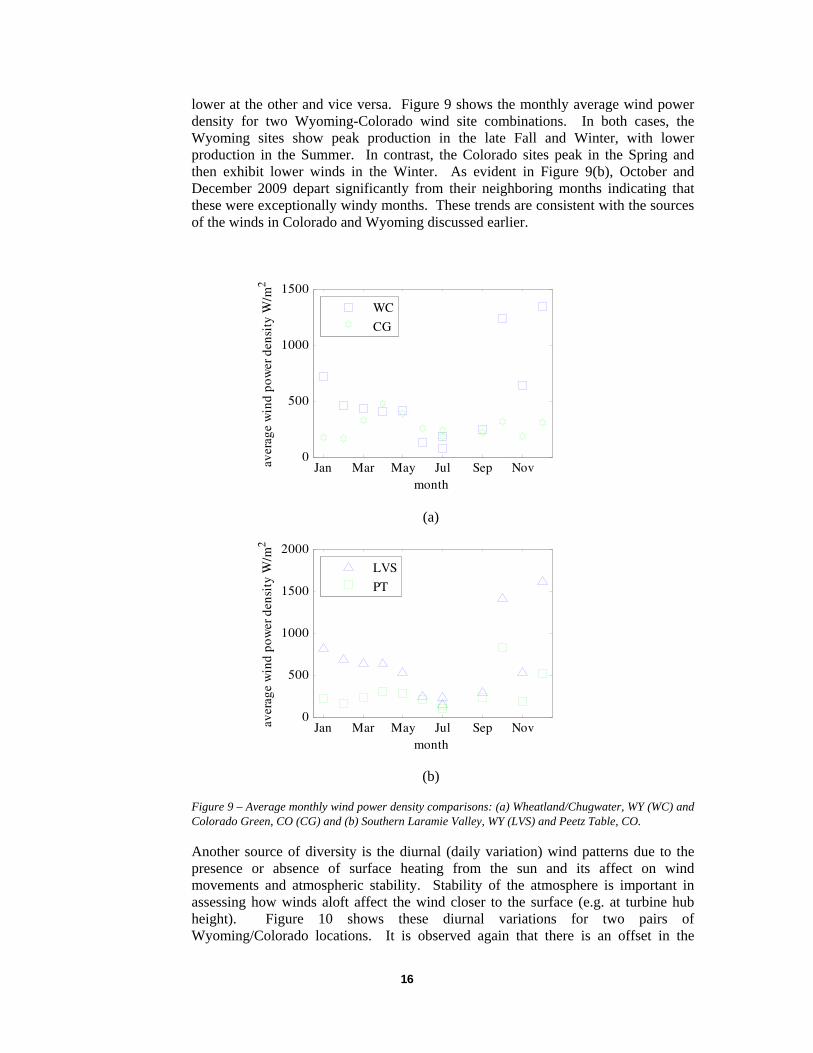
lower at the other and vice versa. Figure 9 shows the monthly average wind power density for two Wyoming-Colorado wind site combinations. In both cases, the Wyoming sites show peak production in the late Fall and Winter, with lower production in the Summer. In contrast, the Colorado sites peak in the Spring and then exhibit lower winds in the Winter. As evident in Figure 9(b), October and December 2009 depart significantly from their neighboring months indicating that these were exceptionally windy months. These trends are consistent with the sources of the winds in Colorado and Wyoming discussed earlier.

(a)

(b)

Figure 9 – Average monthly wind power density comparisons: (a) Wheatland/Chugwater, WY (WC) and Colorado Green, CO (CG) and (b) Southern Laramie Valley, WY (LVS) and Peetz Table, CO.

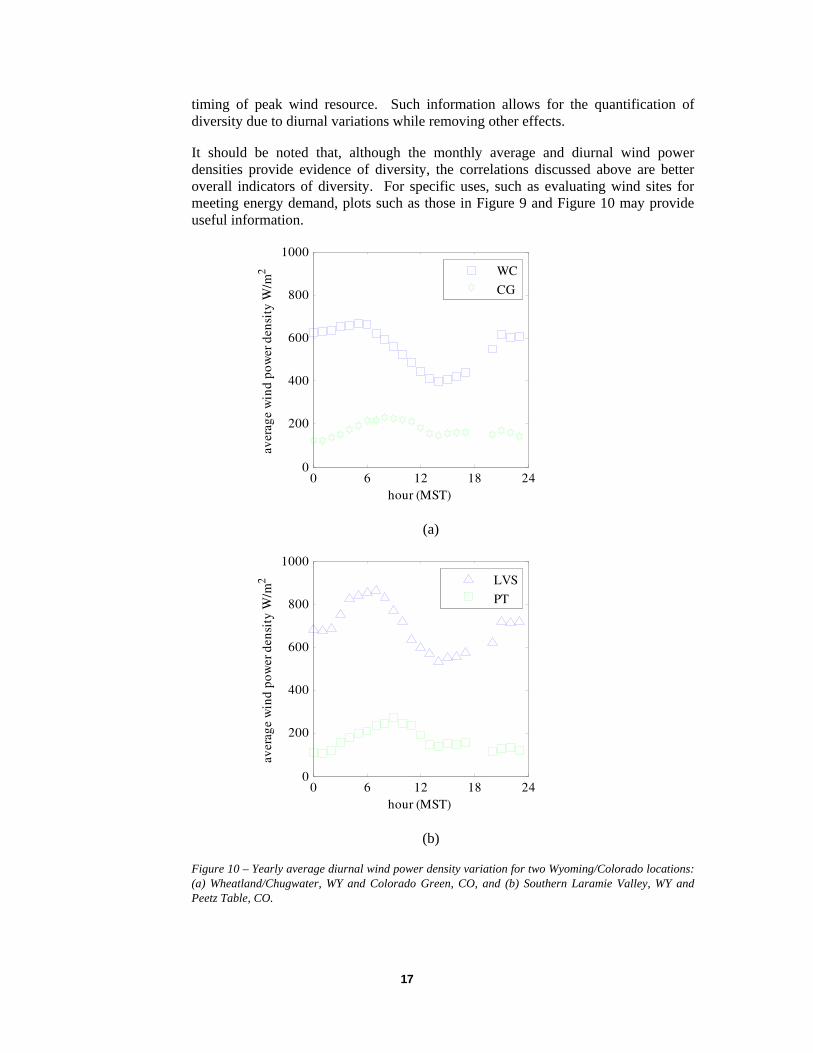
Another source of diversity is the diurnal (daily variation) wind patterns due to the presence or absence of surface heating from the sun and its affect on wind movements and atmospheric stability. Stability of the atmosphere is important in assessing how winds aloft affect the wind closer to the surface (e.g. at turbine hub height). Figure 10 shows these diurnal variations for two pairs of Wyoming/Colorado locations. It is observed again that there is an offset in the

Jan Mar May Jul Sep Nov0

500

1000

1500

month

aver

age

win

d po

wer

den

sity

W/m

2

WC

CG

Jan Mar May Jul Sep Nov0

500

1000

1500

2000

month

aver

age

win

d po

wer

den

sity

W/m

2

LVS

PT

17

timing of peak wind resource. Such information allows for the quantification of diversity due to diurnal variations while removing other effects.

It should be noted that, although the monthly average and diurnal wind power densities provide evidence of diversity, the correlations discussed above are better overall indicators of diversity. For specific uses, such as evaluating wind sites for meeting energy demand, plots such as those in Figure 9 and Figure 10 may provide useful information.

(a)

(b)

Figure 10 – Yearly average diurnal wind power density variation for two Wyoming/Colorado locations: (a) Wheatland/Chugwater, WY and Colorado Green, CO, and (b) Southern Laramie Valley, WY and Peetz Table, CO.

0 6 12 18 240

200

400

600

800

1000av

erag

e w

ind

pow

er d

ensi

ty W

/m2

hour (MST)

WC

CG

0 6 12 18 240

200

400

600

800

1000

aver

age

win

d po

wer

den

sity

W/m

2

hour (MST)

LVS

PT

18

Estimated Wind Power Production for Various Scenarios Once candidate sites are selected from an analysis such as that above, the benefits of diversification can be investigated by considering the power output from different combinations of sites. In order to focus on diversity first, the individual sites were sized such that, in aggregate, they would equally contribute to a certain average power (1000 MW) based on their ideal capacity factor (the capacity factor determined from the modeled wind and turbine model – no accounting for down time, etc.). This also addresses any questions about the modeled data as the variability is the focus rather than the exact wind speeds.

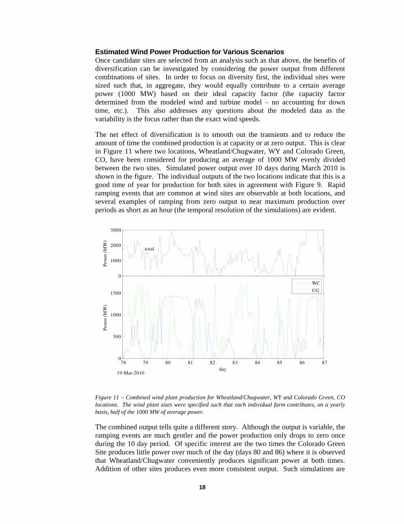
The net effect of diversification is to smooth out the transients and to reduce the amount of time the combined production is at capacity or at zero output. This is clear in Figure 11 where two locations, Wheatland/Chugwater, WY and Colorado Green, CO, have been considered for producing an average of 1000 MW evenly divided between the two sites. Simulated power output over 10 days during March 2010 is shown in the figure. The individual outputs of the two locations indicate that this is a good time of year for production for both sites in agreement with Figure 9. Rapid ramping events that are common at wind sites are observable at both locations, and several examples of ramping from zero output to near maximum production over periods as short as an hour (the temporal resolution of the simulations) are evident.

Figure 11 – Combined wind plant production for Wheatland/Chugwater, WY and Colorado Green, CO locations. The wind plant sizes were specified such that each individual farm contributes, on a yearly basis, half of the 1000 MW of average power.

The combined output tells quite a different story. Although the output is variable, the ramping events are much gentler and the power production only drops to zero once during the 10 day period. Of specific interest are the two times the Colorado Green Site produces little power over much of the day (days 80 and 86) where it is observed that Wheatland/Chugwater conveniently produces significant power at both times. Addition of other sites produces even more consistent output. Such simulations are

78 79 80 81 82 83 84 85 86 870

500

1000

1500

day

Pow

er (M

W)

19-Mar-2010

WC

CG

0

1000

2000

3000

Pow

er (M

W)

total

19

valuable for demonstrating the effects of diversity, but seasonal or yearly measures of the effectiveness of diversity are needed to allow for evaluation of a certain group of wind assets identified for diversity.

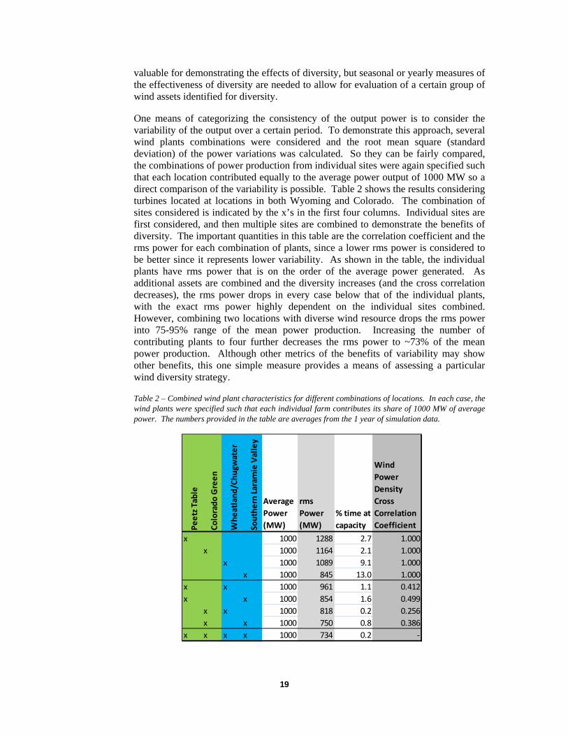
One means of categorizing the consistency of the output power is to consider the variability of the output over a certain period. To demonstrate this approach, several wind plants combinations were considered and the root mean square (standard deviation) of the power variations was calculated. So they can be fairly compared, the combinations of power production from individual sites were again specified such that each location contributed equally to the average power output of 1000 MW so a direct comparison of the variability is possible. Table 2 shows the results considering turbines located at locations in both Wyoming and Colorado. The combination of sites considered is indicated by the x’s in the first four columns. Individual sites are first considered, and then multiple sites are combined to demonstrate the benefits of diversity. The important quantities in this table are the correlation coefficient and the rms power for each combination of plants, since a lower rms power is considered to be better since it represents lower variability. As shown in the table, the individual plants have rms power that is on the order of the average power generated. As additional assets are combined and the diversity increases (and the cross correlation decreases), the rms power drops in every case below that of the individual plants, with the exact rms power highly dependent on the individual sites combined. However, combining two locations with diverse wind resource drops the rms power into 75-95% range of the mean power production. Increasing the number of contributing plants to four further decreases the rms power to ~73% of the mean power production. Although other metrics of the benefits of variability may show other benefits, this one simple measure provides a means of assessing a particular wind diversity strategy.

Table 2 – Combined wind plant characteristics for different combinations of locations. In each case, the wind plants were specified such that each individual farm contributes its share of 1000 MW of average power. The numbers provided in the table are averages from the 1 year of simulation data.

Peetz Table

Colorado Green

Wheatland/Chugw

ater

Southern Laram

ie Valley

Average 

Power 

(MW)

rms 

Power 

(MW)

% time at 

capacity

Wind 

Power 

Density 

Cross 

Correlation 

Coefficient

x 1000 1288 2.7 1.000

x 1000 1164 2.1 1.000

x 1000 1089 9.1 1.000

x 1000 845 13.0 1.000

x x 1000 961 1.1 0.412

x x 1000 854 1.6 0.499

x x 1000 818 0.2 0.256

x x 1000 750 0.8 0.386

x x x x 1000 734 0.2 ‐

20

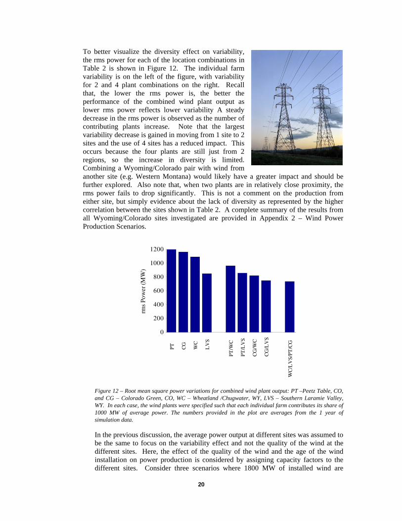
To better visualize the diversity effect on variability, the rms power for each of the location combinations in Table 2 is shown in Figure 12. The individual farm variability is on the left of the figure, with variability for 2 and 4 plant combinations on the right. Recall that, the lower the rms power is, the better the performance of the combined wind plant output as lower rms power reflects lower variability A steady decrease in the rms power is observed as the number of contributing plants increase. Note that the largest variability decrease is gained in moving from 1 site to 2 sites and the use of 4 sites has a reduced impact. This occurs because the four plants are still just from 2 regions, so the increase in diversity is limited. Combining a Wyoming/Colorado pair with wind from another site (e.g. Western Montana) would likely have a greater impact and should be further explored. Also note that, when two plants are in relatively close proximity, the rms power fails to drop significantly. This is not a comment on the production from either site, but simply evidence about the lack of diversity as represented by the higher correlation between the sites shown in Table 2. A complete summary of the results from all Wyoming/Colorado sites investigated are provided in Appendix 2 – Wind Power Production Scenarios.

Figure 12 – Root mean square power variations for combined wind plant output: PT –Peetz Table, CO, and CG – Colorado Green, CO, WC – Wheatland /Chugwater, WY, LVS – Southern Laramie Valley, WY. In each case, the wind plants were specified such that each individual farm contributes its share of 1000 MW of average power. The numbers provided in the plot are averages from the 1 year of simulation data.

In the previous discussion, the average power output at different sites was assumed to be the same to focus on the variability effect and not the quality of the wind at the different sites. Here, the effect of the quality of the wind and the age of the wind installation on power production is considered by assigning capacity factors to the different sites. Consider three scenarios where 1800 MW of installed wind are

0

200

400

600

800

1000

1200

rms

Pow

er (M

W)

PT CG

WC

LV

S

PT/W

C

PT/L

VS

CG

/WC

CG

/LV

S

WC

/LV

S/PT

/CG

21

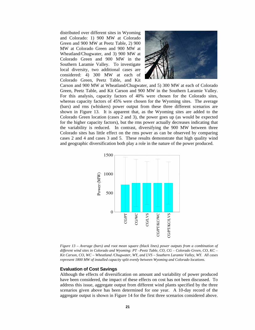
distributed over different sites in Wyoming and Colorado: 1) 900 MW at Colorado Green and 900 MW at Peetz Table, 2) 900 MW at Colorado Green and 900 MW at Wheatland/Chugwater, and 3) 900 MW at Colorado Green and 900 MW in the Southern Laramie Valley. To investigate local diversity, two additional cases are considered: 4) 300 MW at each of Colorado Green, Peetz Table, and Kit Carson and 900 MW at Wheatland/Chugwater, and 5) 300 MW at each of Colorado Green, Peetz Table, and Kit Carson and 900 MW in the Southern Laramie Valley. For this analysis, capacity factors of 40% were chosen for the Colorado sites, whereas capacity factors of 45% were chosen for the Wyoming sites. The average (bars) and rms (whiskers) power output from these three different scenarios are shown in Figure 13. It is apparent that, as the Wyoming sites are added to the Colorado Green location (cases 2 and 3), the power goes up (as would be expected for the higher capacity factors), but the rms power actually decreases indicating that the variability is reduced. In contrast, diversifying the 900 MW between three Colorado sites has little effect on the rms power as can be observed by comparing cases 2 and 4 and cases 3 and 5. These results demonstrate that high quality wind and geographic diversification both play a role in the nature of the power produced.

Figure 13 – Average (bars) and root mean square (black lines) power outputs from a combination of different wind sites in Colorado and Wyoming: PT –Peetz Table, CO, CG – Colorado Green, CO, KC – Kit Carson, CO, WC – Wheatland /Chugwater, WY, and LVS – Southern Laramie Valley, WY. All cases represent 1800 MW of installed capacity split evenly between Wyoming and Colorado locations.

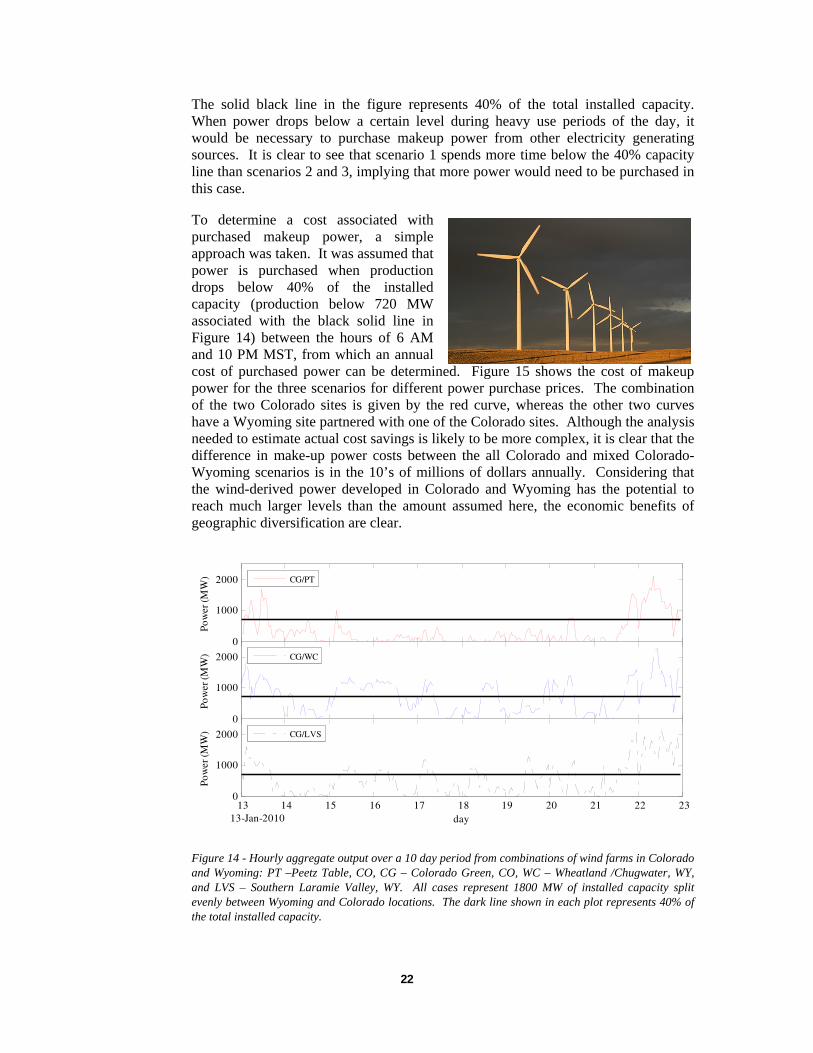
Evaluation of Cost Savings Although the effects of diversification on amount and variability of power produced have been considered, the impact of these effects on cost has not been discussed. To address this issue, aggregate output from different wind plants specified by the three scenarios given above has been determined for one year. A 10-day record of the aggregate output is shown in Figure 14 for the first three scenarios considered above.

0

500

1000

1500

Pow

er (M

W)

CG

/PT

CG

/WC

CG

/LV

S

CG

/PT

/KC

/WC

CG

/PT

/KC

/LV

S

22

The solid black line in the figure represents 40% of the total installed capacity. When power drops below a certain level during heavy use periods of the day, it would be necessary to purchase makeup power from other electricity generating sources. It is clear to see that scenario 1 spends more time below the 40% capacity line than scenarios 2 and 3, implying that more power would need to be purchased in this case.

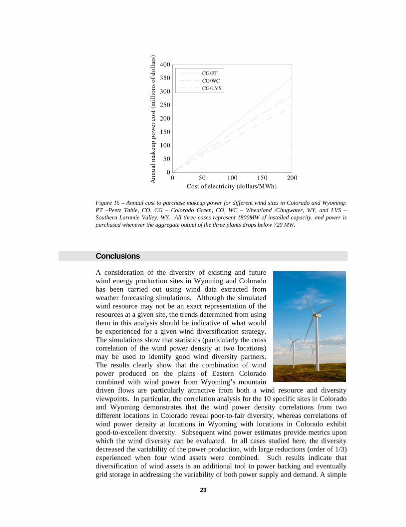
To determine a cost associated with purchased makeup power, a simple approach was taken. It was assumed that power is purchased when production drops below 40% of the installed capacity (production below 720 MW associated with the black solid line in Figure 14) between the hours of 6 AM and 10 PM MST, from which an annual cost of purchased power can be determined. Figure 15 shows the cost of makeup power for the three scenarios for different power purchase prices. The combination of the two Colorado sites is given by the red curve, whereas the other two curves have a Wyoming site partnered with one of the Colorado sites. Although the analysis needed to estimate actual cost savings is likely to be more complex, it is clear that the difference in make-up power costs between the all Colorado and mixed Colorado-Wyoming scenarios is in the 10’s of millions of dollars annually. Considering that the wind-derived power developed in Colorado and Wyoming has the potential to reach much larger levels than the amount assumed here, the economic benefits of geographic diversification are clear.

Figure 14 - Hourly aggregate output over a 10 day period from combinations of wind farms in Colorado and Wyoming: PT –Peetz Table, CO, CG – Colorado Green, CO, WC – Wheatland /Chugwater, WY, and LVS – Southern Laramie Valley, WY. All cases represent 1800 MW of installed capacity split evenly between Wyoming and Colorado locations. The dark line shown in each plot represents 40% of the total installed capacity.

0

1000

2000

Pow

er (M

W)

CG/PT

0

1000

2000

Pow

er (M

W)

CG/WC

13 14 15 16 17 18 19 20 21 22 230

1000

2000

day

Pow

er (M

W)

13-Jan-2010

CG/LVS

23

Figure 15 – Annual cost to purchase makeup power for different wind sites in Colorado and Wyoming: PT –Peetz Table, CO, CG – Colorado Green, CO, WC – Wheatland /Chugwater, WY, and LVS – Southern Laramie Valley, WY. All three cases represent 1800MW of installed capacity, and power is purchased whenever the aggregate output of the three plants drops below 720 MW.

Conclusions

A consideration of the diversity of existing and future wind energy production sites in Wyoming and Colorado has been carried out using wind data extracted from weather forecasting simulations. Although the simulated wind resource may not be an exact representation of the resources at a given site, the trends determined from using them in this analysis should be indicative of what would be experienced for a given wind diversification strategy. The simulations show that statistics (particularly the cross correlation of the wind power density at two locations) may be used to identify good wind diversity partners. The results clearly show that the combination of wind power produced on the plains of Eastern Colorado combined with wind power from Wyoming’s mountain driven flows are particularly attractive from both a wind resource and diversity viewpoints. In particular, the correlation analysis for the 10 specific sites in Colorado and Wyoming demonstrates that the wind power density correlations from two different locations in Colorado reveal poor-to-fair diversity, whereas correlations of wind power density at locations in Wyoming with locations in Colorado exhibit good-to-excellent diversity. Subsequent wind power estimates provide metrics upon which the wind diversity can be evaluated. In all cases studied here, the diversity decreased the variability of the power production, with large reductions (order of 1/3) experienced when four wind assets were combined. Such results indicate that diversification of wind assets is an additional tool to power backing and eventually grid storage in addressing the variability of both power supply and demand. A simple

0 50 100 150 2000

50

100

150

200

250

300

350

400

Cost of electricity (dollars/MWh)

Ann

ual m

akeu

p po

wer

cos

t (m

illi

ons

of d

olla

rs)

CG/PTCG/WCCG/LVS

24

analysis considering the cost of buying power when 1800 MW of installed wind energy capacity fail to produce a sufficient amount of power indicated savings in the 10s of millions of dollars are possible through geographic diversification.

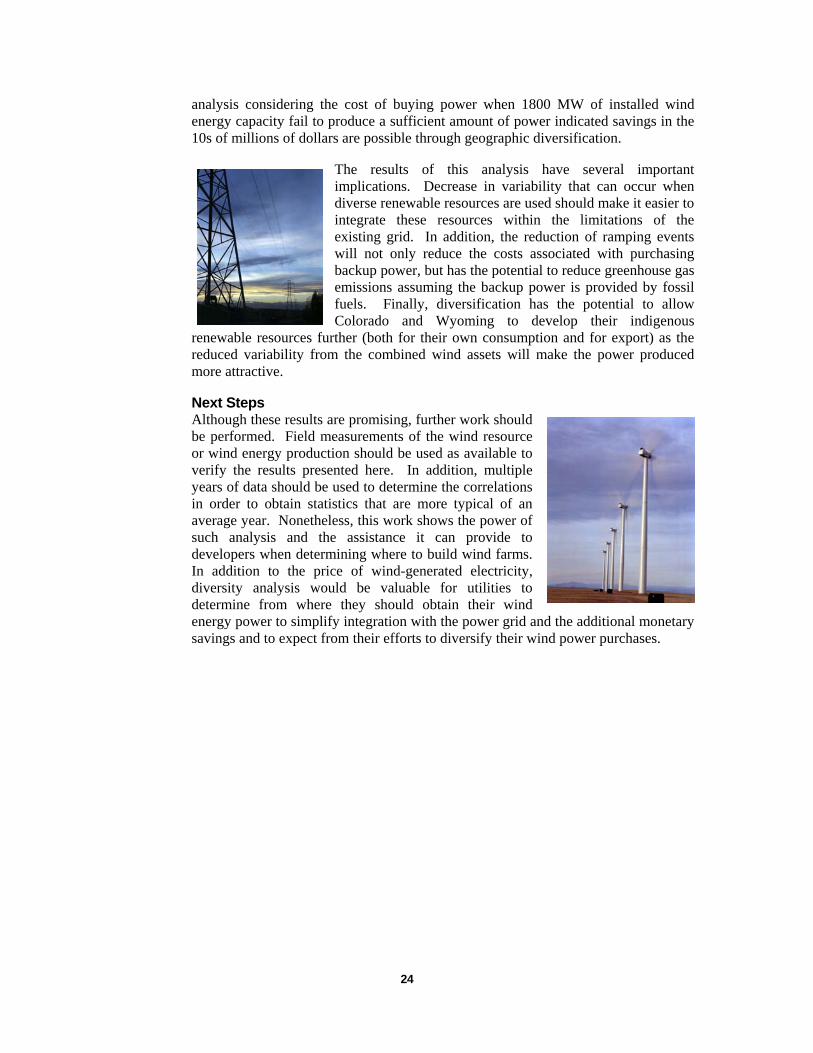
The results of this analysis have several important implications. Decrease in variability that can occur when diverse renewable resources are used should make it easier to integrate these resources within the limitations of the existing grid. In addition, the reduction of ramping events will not only reduce the costs associated with purchasing backup power, but has the potential to reduce greenhouse gas emissions assuming the backup power is provided by fossil fuels. Finally, diversification has the potential to allow Colorado and Wyoming to develop their indigenous

renewable resources further (both for their own consumption and for export) as the reduced variability from the combined wind assets will make the power produced more attractive.

Next Steps Although these results are promising, further work should be performed. Field measurements of the wind resource or wind energy production should be used as available to verify the results presented here. In addition, multiple years of data should be used to determine the correlations in order to obtain statistics that are more typical of an average year. Nonetheless, this work shows the power of such analysis and the assistance it can provide to developers when determining where to build wind farms. In addition to the price of wind-generated electricity, diversity analysis would be valuable for utilities to determine from where they should obtain their wind energy power to simplify integration with the power grid and the additional monetary savings and to expect from their efforts to diversify their wind power purchases.

25

References

1 Wind Powering America, Colorado Wind Map and Wind Resource Potential, http://www.windpoweringamerica.gov/wind_resource_maps.asp?stateab=co .

2 Wind Powering America, Wyoming Wind Map and Wind Resource Potential, http://www.windpoweringamerica.gov/wind_resource_maps.asp?stateab=wy .

3 Database of State Incentives for Renewables and Efficiency (DSIRE), http://www.dsireusa.org/.

4 J. Naughton, J. Baker, and T. Parish, “Wind Diversity in Wyoming,” Wind Energy Research Center Report, WERC-2012-1, July 2012.

5N.J. Doesken, R.A. Pielke Sr., and O.A.P. Bliss, “Climate of Colorado”, Climatography of the United States, No. 60, January 2003.

6 J.S. Bendat and A.G. Piersol, Random Data Analysis, 2nd Edition, John Wiley and Sons, New York, pp.109-113.

26

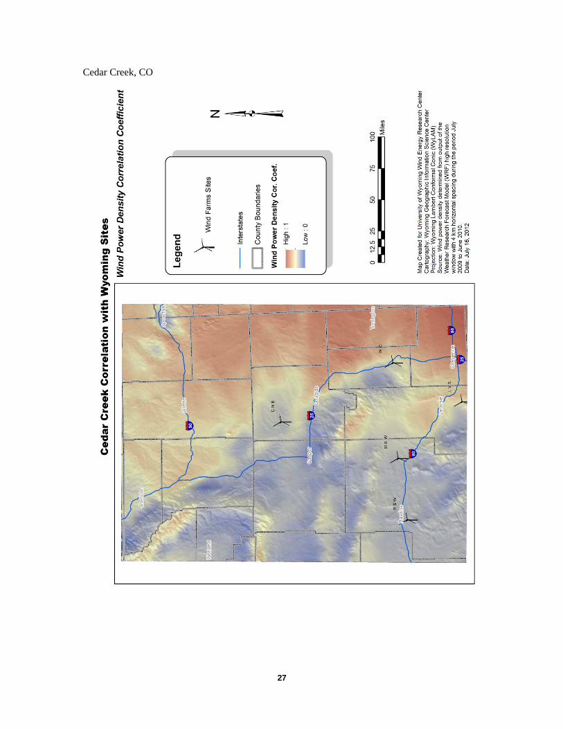
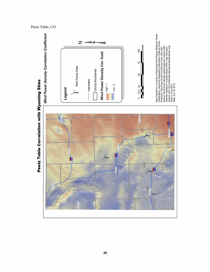
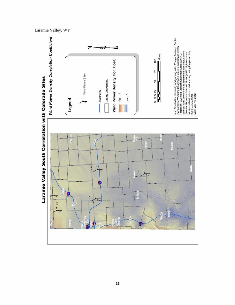
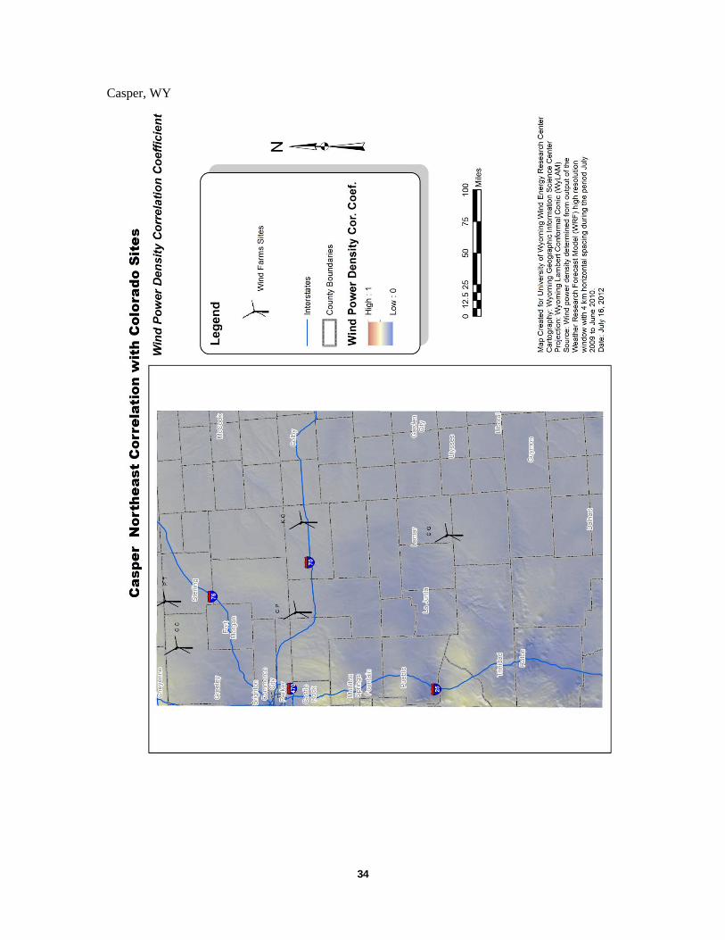
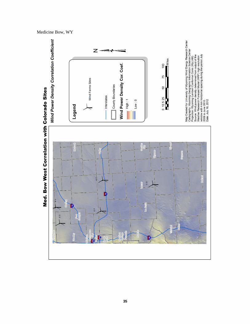
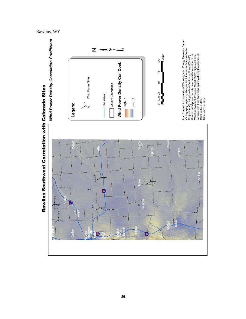
Appendix 1 – Wind Correlation Maps

A limited number of wind correlations maps were provided in the main text. Below, a complete set of correlation maps corresponding to each of the Wyoming and Colorado wind sites chosen is provided. To facilitate their use, each is provided as a standalone graphic.

27

Cedar Creek, CO

28

Peetz Table, CO

29

Kit Carson, CO

30

Cedar Point, CO

31

Colorado Green, CO

32

Wheatland/Chugwater, WY

33

Laramie Valley, WY

34

Casper, WY

35

Medicine Bow, WY

36

Rawlins, WY

37

Appendix 2 – Wind Power Production Scenarios

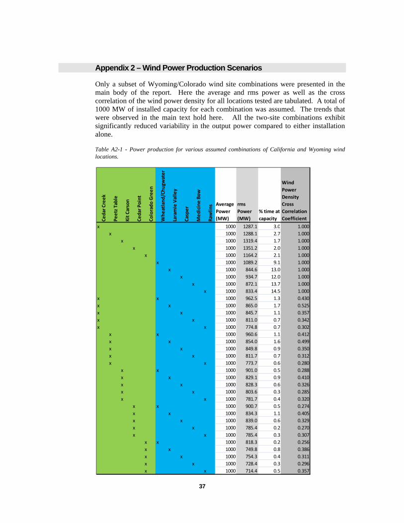
Only a subset of Wyoming/Colorado wind site combinations were presented in the main body of the report. Here the average and rms power as well as the cross correlation of the wind power density for all locations tested are tabulated. A total of 1000 MW of installed capacity for each combination was assumed. The trends that were observed in the main text hold here. All the two-site combinations exhibit significantly reduced variability in the output power compared to either installation alone.

Table A2-1 - Power production for various assumed combinations of California and Wyoming wind locations.

Cedar Creek

Peetz Table

Kit Carson

Cedar Point

Colorado Green

Wheatland/Chugw

ater

Laramie Valley

Casper

Medicine Bow

Raw

lins Average 

Power 

(MW)

rms 

Power 

(MW)

% time at 

capacity

Wind 

Power 

Density 

Cross 

Correlation 

Coefficient

x 1000 1287.1 3.0 1.000

x 1000 1288.1 2.7 1.000

x 1000 1319.4 1.7 1.000

x 1000 1351.2 2.0 1.000

x 1000 1164.2 2.1 1.000

x 1000 1089.2 9.1 1.000

x 1000 844.6 13.0 1.000

x 1000 934.7 12.0 1.000

x 1000 872.1 13.7 1.000

x 1000 833.4 14.5 1.000

x x 1000 962.5 1.3 0.430

x x 1000 865.0 1.7 0.525

x   x 1000 845.7 1.1 0.357

x x 1000 811.0 0.7 0.342

x x 1000 774.8 0.7 0.302

x x 1000 960.6 1.1 0.412

x x 1000 854.0 1.6 0.499

x   x 1000 849.8 0.9 0.350

x x 1000 811.7 0.7 0.312

x x 1000 773.7 0.6 0.280

x x 1000 901.0 0.5 0.288

x x 1000 829.1 0.9 0.410

x   x 1000 828.3 0.6 0.326

x x 1000 803.6 0.3 0.285

x x 1000 781.7 0.4 0.320

x x 1000 900.7 0.5 0.274

x x 1000 834.3 1.1 0.405

x   x 1000 839.0 0.6 0.329

x x 1000 785.4 0.2 0.270

x x 1000 785.4 0.3 0.307

x x 1000 818.3 0.2 0.256

x x 1000 749.8 0.8 0.386

x   x 1000 754.3 0.4 0.311

x x 1000 728.4 0.3 0.296

x x 1000 714.4 0.5 0.357