Wind turbine wake properties : Comparison between anon-rotating simplified wind turbine model and a

rotating model

S. Aubrun1, S. Loyer1, P. E. Hancock2 and P. Hayden2

1 Laboratoire PRISME, Universite d’Orleans8 rue Leonard de Vinci F-45072 Orleans Cedex 2, France

2 EnFlo Laboratory, University of Surrey, Surrey, UK

Abstract

Experimental results on the wake properties of a non-rotating simplified windturbine model, based on the actuator disc concept, and a rotating model, athree-blade wind turbine, are presented. Tests were performed in two differ-ent facilities, one providing a nominally Decaying Isotropic Turbulent inflow(turbulence intensity of 4% at rotor disc location) and one providing a neutralatmospheric boundary layer above a moderately rough terrain at a geometricscale of 1 : 300 (determined from the combination of several indicators), with13% of turbulence intensity at hub height). The objective is to determine thelimits of the simplified wind turbine model to reproduce a realistic wind turbinewake. Pressure and high-order velocity statistics are therefore compared in thewake of both rotor discs for two different inflow conditions in order to quan-tify the influence of the ambient turbulence. It has been shown that wakes ofrotating model and porous disc developing in the modelled atmospheric bound-ary layer are indistinguishable after 3 diameters downstream of the rotor discs,whereas few discrepancies are still visible at the same distance with the DecayingIsotropic Turbulent inflow.

Key words: Porous disc, Wind turbine, Wake, Homogeneous and IsotropicTurbulent flow, Atmospheric Boundary Layer flow, wind tunnel

1. Introduction

In order to study the wind turbine wake and its eventual interactions withneighbouring wind turbines, several numerical and physical modelling approachesare used. Some model the wind turbine with the simplest model, which is theactuator disc concept, adding a drag source (i.e. pressure loss) within the sur-face swept by the blades (exemples for numerical [1] and physical applications[5, 2, 3, 11, 10]). Some use the Blade Element Momentum Theory, which takesinto account the blade rotation effect on the wake and the aerodynamic featuresof the blades [13, 6]. Some use Reynolds-Averaged-Navier-Stokes simulation

Preprint submitted to Journal of Wind Engineering and Industrial AerodynamicsMarch 27, 2013

or Large-Eddy-Simulation to compute the steady and unsteady flows throughmodelled or real rotors [16, 15, 19]. In a wind resource assessment context, thelatter one is not practical enough to be used since the computation times areextremely long, even if it delivers the better results with respect to the insta-tionary process. Consequentely, RANS simulation is still the most attractiveto model the far wake, according to its simplicity of implementation and shortcomputation time. On the other hand, the issue is that it is difficult to assessthe errors induced by the absence of blades and associated rotation momentumon the wake development. Furthermore, the level of turbulence intensity en-countered in the atmospheric incoming flow plays a role on this issue : First,the higher the turbulence intensity is, the faster the spectral signature of theblades disappears in the wake and the faster the tangential velocity inducedby the rotational momentum is overwhelmed in ambiant velocity fluctuations.These observations need to be quantified. In this context, the present studycompares the wake properties of a model of a three-blade rotating wind turbine[14] and of a porous disc made of metallic mesh, generating the same velocitydeficit as the wind turbine. Both models are tested in a modelled atmosphericboundary layer flow and in a Decaying Isotropic Turbulent flow in order tosee the influence of the approach flow conditions. The velocity statistics arecompared between both models in order to determine whether the far wakestate is reached at x = 3D. Here, the far wake is defined by the self-similarityof the velocity deficit and turbulence intensity profiles downstream of models(Gaussian-type distributions). The spectral content of the flow is also studiedin order to determine whether the blade signature in the wake is still visible atthis location.

2. Experimental set-up

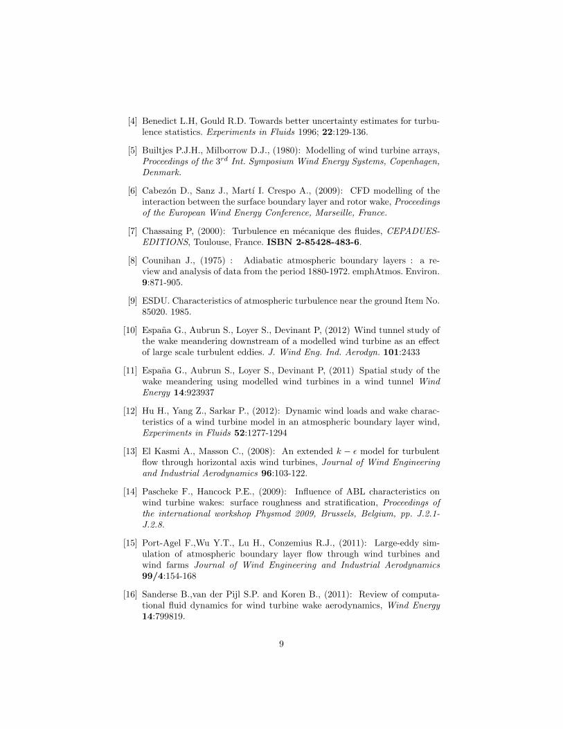
In this study, all measurements are performed in the closed circuit windtunnel of the PRISME laboratory (Fig. 1). This facility is equipped with twotest sections. The main one is 2m high, 2m wide and 5m long and is used inthe present study to generate Decaying ’Isotropic’ Turbulent flow. The secondone is 5m high, 5m wide and 20m long and is located in the return circuit ofthe wind tunnel. It is used in the present study to reproduce the properties ofa neutral ABL at a reduced scale. To generate the Decaying ’Isotropic’ Turbu-lence, denoted DIT, a turbulence grid is placed at the entrance of themain testsection. The turbulence grid is made of metallic square section 25mm× 25mmbars with a mesh size of 100mm. The reference velocity and turbulence inten-sity (indicated with index 0) are measured at the rotor disc location, but inabsence of it. They are U0 = 2.5m/s and Iu0 = 4%, respectively. Iu is definedas the ratio between the standard deviation of streamwise velocity u′ and itstime average U . The ratio of standard deviations v′/u′ and w′/u′ are 1.06 and1.03, respectively. This indicates the isotropy of the approach flow.

The flow in the return circuit is tuned by pre-defined installations in theflow processing unit upstream the test section resulting in a modelled moder-

2

ately rough ABL (Roughness length z0 = 0.03mm in wind tunnel scale, powerlaw coefficient α = 0.14). The geometric scale of 1 : 300 is deduced from thebest fit between wind tunnel data and literature about neutral ABL regardingthe expected roughness length range, turbulence intensity profiles and integrallength scale profiles [8, 9, 17, 20]. At z = 300mm (hub height), the upstreammean velocity is U0 = 2.5m/s and the turbulence intensity is Iu0 = 13% (Figure2). According to experimental limitations, the velocity profile is measured upto 900mm above ground. Results show that the boundary layer limit is no yetreached at this altitude.The 3-blade rotating wind turbine (Fig. 3) has a diameter D = 416mm, itsrotation is controlled and its tip-speed-ratio is fixed to TSR = 5.8. the work ofSunada et al. [18] has shown that at such low chord Reynolds numbers, standardaerofoil profiles do not behave as they do at high Reynolds numbers. They alsoshowed that thin plate aerofoils behave more like aerofoils at high Reynoldsnumber, except that they stall at a lower lift coefficient. Consequently, theblades were designed according to this statement [14].The thrust coefficient CT had been experimentally assessed at CT = 0.5 in auniform inflow, using the global momentum theory. Knowing the velocity deficitdistribution downstream of the rotor U0 − U(r), the axial force acting on therotor is obtained by integrating the momentum flux crossing a reference surface :

Fax = 2π

∫ ∞

0

ρU(r)(U0 − U(r)

)rdr (1)

The thrust coefficient is then defined as:

CT =Fax

12ρU

20SD

(2)

Pascheke and Hancock [14] presented the velocity deficit and turbulence in-tensity distributions downstream of this rotating wind turbine located in mod-elled onshore and offshore boundary layers. The values of maximum velocitydeficit (40 to 50% of the mean hub velocity) are representative of full scale windturbine wakes and are in agreement with literature [21, 24, 22]. Since the wakediffusion is dependent of the boundary layer conditions, it is difficult de preciselycompare the wake evolution obtained in the latter references. Nevertheless, thetrend is in agreement, showing some self-similar profiles for the velocity deficitand the turbulence intensity in the far wake (from x/D = 3 to 5, depending onthe terrain roughness and/or thermal stability).

A porous disc made of metallic mesh (Fig. 4) is designed in order to repro-duce the same velocity deficit at x = 0.5D downstream of the disc as downstreamof the 3-blade rotating wind turbine. Even if the velocity deficit was the onlydesing criterion, it was nevertheless expected that, if both velocity deficits fit-ted, the turbulence intensity profiles were similar in areas where the turbulenceproduction is due to velocity gradients (external wake boundaries and hub). On

3

the other hand, areas where the turbulence production is due to the grid for theporous disc or to the blade transit for the rotating wind turbine, it is expectedto have discrepancies at this short distance downstream of the rotor discs. Oneof the main reasons of choosing meshes to reproduce the actuator disc at re-duced scale in a wind tunnel is that the porous disc can be considered as a gridturbulence generator. This set-up is known to be Reynolds number independent[7]. The porous disc has the same diameter as the wind turbine, the mesh hasa solidity of 45% and a circle of different solidity (35%) of diameter 0.2D fixedat the center of the main disc. The choice of solidities was driven by a previousparametrical study [2]. The disc is fixed on a mast to be located at the sameheight as the wind turbine rotor.x, y and z coordinate origins are located at the rotor center. x is the streamwisedirection, y is the transverse one and z, the vertical one.The difference of the static pressure in the flow, ∆Ps, is measured as the dif-ference of the static pressure in the wake flow of the rotor disc, Ps, and thestatic pressure of the free undisturbed flow, Pext, at least 1m above the rotordisc (∆Ps = Ps − Pext). Each static pressure is measured through the staticbranch of a Pitot tube and the static pressure difference ∆Ps is measured witha DRUCK 0-25 Pa differential pressure transducer with an acquisition time of180s. The 3D flow properties are measured from x = 0.5D to 3D downstreamof the wind turbine with a triple-sensor gold-plated wire probe (Dantec 55P91).It is controlled with a Dantec Streamline CTA system, the sampling frequencyis fixed to 6kHz and the acquisition time to 180s. The used triple-sensor wireprobe is able to measure a velocity vector with an acceptance cone of 70.4.According to our measurements, the maximal angle between the streamwisedirection and the velocity vector is obtained in DIT conditions at x/D = 0.5,where the rotational momentum is the highest (W/U0 = 0.18 and U/U0 = 0.55)and is assessed to a measurement cone of 36 on average, and 62 instantaneously(assuming a maximal instantaneous velocity of (W +Wrms)/U0 = 0.33). Theroot-mean-square errors of the measured velocity statistics were assessed for theABL configuration at the worst location (i.e. the worst case: highest turbulenceintensity 27% and largest integral scales 0.5m). For a 95% confidence interval,3.3% error is obtained for the mean velocity, 8.7% for the root-mean-squarevelocity, 30% for the skewness and 121% for the Kurtosis [4]. These statisticalerrors are reduced to 0.7%, 3.3%, 11.3% and 45.3%, respectively, for the DITconfiguration at the worst location.

3. Results and discussion

3.1. Static pressure evolution

The static pressure coefficient (Cp = (Ps −Pext)/(0.5ρU20 )) evolution down-

stream of both rotor discs can be deduced from the static pressure measurementsmentioned in the previous part. Figure 5 shows this information at two differ-ent transverse locations : at the center (y/D = z/D = 0) and at half radius

4

(y/D = 0.25, z/D = 0) of the rotor discs for DIT flow conditions. According tothe uniform approach flow, axisymmetry is assumed. The trends and the levelsof all curves are similar. The pressure coefficients are negative close to the rotordiscs, due to the global energy extraction, tends to zero up to x/D = 1.5, andstays around zero further downstream. This proofs that the pressure recoveryis reached at this distance. For the porous disc, the static pressure coefficientevolution along the x axis is similar for both transverse locations except veryclose to the disc, where the pressure loss is slightly lower at the center than athalf radius. It illustrates that the energy extraction is lower at the center sincethe local mesh solidity is lower. On the other hand, this discrepancy disappearsvery quickly. Making an extrapolation of the Cp to x/D = 0, giving Cp of about-0.26, actuator disc theory implies a CT of 0.59. A CT of 0.5 would require Cp

to be -0.23. Nevertheless, according to the measurement uncertainty due to theuse of a static pressure probe in an unsteady and turbulent flow, this result canbe considered as acceptable.

For the wind turbine, the pressure loss is higher at the center than at halfradius. It is possibly due to the hub wake effect. At the center, the pressurerecovery needs consequentely slightly longer distance to be reached . To con-clude on this part, the pressure recovery downstream the porous disc and thewind turbine is very similar and is reached at x/D = 1.5. It is a first steptowards the proof of similarity between the wind turbine and the porous discwake. Additionally, it confirms that the assumption of pressure recovery that isimplicitely used in the computation of the thrust coefficient through the use ofglobal momentum theory is valid.

3.2. Velocity statistic comparison

Velocity statistics (time-mean , RMS, skewness and Kurtosis) are compared.Figures 6 and 7 show the dimensionless streamwise mean velocity deficit ((U0−U(y))/U0) profiles versus the spanwise direction y/D, at x/D = 0.5 and 3downstream of the porous disc and of the wind turbine. As seen on Figures,the porous disc has been correctly designed since since a sufficient similaritybetween both wakes is established at x/D = 0.5 x/D = 0.5. Indeed, the velocitydeficit distribution within the wakes is slightly different since the disc porosityis uniform, but the discrepancies do not distort too much the velocity gradientsat the wake edges. Farther downstream at x/D = 3, the wakes, which freelydevelop, become completely similar for both inflow conditions. Figures 8 and 9show the streamwise turbulence intensity profiles versus the spanwise directiony/D, at x/D = 0.5 and 3 downstream of the porous disc and of the windturbine. Regarding the turbulence intensity profiles, it is clear that they showsome differences at x/D = 0.5 due to discrepancies in turbulence production. Inthe wake of the porous disc, the turbulence production is confined to the edgesof the wake, in the annular shear layer due to the existence of a velocity deficit.The mesh itself does not generate significant added turbulence.

A production of turbulence is also visible at the location where the disc poros-ity changes, due to the associated velocity gradient. In the wake of the wind

5

turbine, these latter sources are visible but the turbulence from the wakes ofthe blades is also noticeable in the middle part of the wake. On the other hand,these discrepancies in turbulence intensity distribution between both wakes havevanished at x/D = 3 due to the turbulence diffusion. They are even totally sup-pressed in the ABL inflow conditions.

The measurement locations were rather close from the rotor discs (maximum3D downstream) and did not enable us to characterize whether the wake recoveryis faster in higher turbulent configurations (as shown in [22]).Nevertheless, thevelocity deficit and turbulence intensity profiles present the typical Gaussian-type distribution representative of the far-wake definition only for the higherturbulent configuration (ABL).

Higher-order statistics, as Skewness and Kurtosis of streamwise velocity fluc-tuations, are also compared on Figures 10, 11, 12 and 13. In DIT conditions,the probability density function of streamwise velocity fluctuations is expectedto be of Gaussian type (skewness equal to zero and Kurtosis equal to 3). Fig-ures 10 and 12 validate these expectations out of the wake disturbance area. InABL flow conditions, the vertical gradient of the streamwise velocity modifiesthe turbulence properties, which are not described anymore by a Gaussian-typePDF function and lead to different skewness and kurtosis values than 0 and3, respectively, even in undisturbed areas (see Figs 11 and 13. In both inflowconfigurations, in the near-wake, the skewness and Kustosis values vary veryrapidly in strong velocity gradient areas and trends are relatively differents forporous disc and the wind turbine. On the other hand, at x/D = 3, the trendsare very similar in all configurations, and discrepancies disappear almost en-tirely in ABL flow conditions.

The last check concerns the streamwise integral length scales Lux(Figures14 and 15). They were calculated by integrating the autocorrelation function ofthe streamwise velocity time series according to the time delay, up to the firstzero crossing. It is important to notice that the order of magnitude of integrallength scales is completely different according to the inflow conditions (ratio of10 between the length scales measured at the rotor disc location but in absenceof it, in ABL and in DIT conditions). In DIT conditions at x/D = 0.5, theintegral length scale is on average 0.05m outside of the wake and is forced to0.02m by the porous disc mesh within the disc wake.

For the rotating wind turbine, the integral length scale is more scatteredbut stays at a comparable level. In ABL conditions at x/D = 0.5, the integrallength scales are also scattered but are also comparable for both wind turbinemodels. It shows that the integral length scale is dominantely driven by theupstream turbulent flow properties rather than by the wind turbine model dis-turbance. Further downstream, in both inflow conditions, the integral lengthscales are quite similar, even if values are sligthly smaller within the wake of therotating wind turbine. Knowing the relative difficulty to interpret the absolutevalue of the integral length scales in non-isotropic flows, one can conclude thatthese are not significant discrepancies with respect to the simulation of the wake

6

flow behind a wind turbine.

To conclude on this part, it is shown that, in relatively high turbulent inflowconditions (ABL conditions here), no significant difference is visible in the wakedescription of a porous disc or of a rotating wind turbine, regarding the fourfirst moments of distribution functions of velocity fluctuations (mean, standarddeviation, Skewness, Kurtosis) and the integral length scales, at a downstreamdistance of x/D = 3. On the other hand, discrepancies still exist at x/D = 3 inlow turbulent inflow conditions (DIT conditions) but are relatively minor so onecan assume sufficient similarity between the porous disc and the wind turbinewake.

3.3. Rotational momentum persistence

In order to check whether the rotational momentum induced by the rota-tion of the wind turbine is still visible in the far-wake of the wind turbine,Fig. 16 presents the horizontal profile of the mean dimensionless vertical veloc-ity (W (y)/U0), downstream of the counter-clockwise rotating wind turbine, forboth inflow configurations. It shows that the velocity signature of the rotationof the global wake is visible in the near-wake of the wind turbine but becomesinsignificant at x/D = 3 at hub height for ABL inflow conditions. It shows that,if the ambient turbulence level is high enough, the turbulent diffusion, respon-sible of the turbulence mixing, destroys the coherence of the rotational flow.These results are consistent with Zhang et al, 2012 [23], who obtained similarconclusions in a neutral incoming boundary layer with a turbulence intensity of8% at hub height.

Again, one can conclude that, in relatively high turbulent inflow conditions(ABL conditions here), the rotational momentum generated by the blade rota-tion is smoothed out in the far wake through turbulent diffusion, eliminatingthe difference between the wake of a porous disc and of a rotating wind turbine.

3.4. Tip-vortex signature persistence

One other remaining question is related to the persistence of the tip-vortexsignature in the wake of a wind turbine. The streamwise velocity Power Spec-tral Density downstream of the wind turbine has been determined across thewake. An example of three different spectra is presented on Fig. 17 for DITinflow conditions and on Fig. 18 for ABL inflow conditions. Velocity time seriesare acquired at hub height but at the wake borders y/D = −0.5, z/D = 0 attwo downstream locations. At x/D = 0.5, two frequency peaks are noticeableat the rotation frequency f = f0 (with f0 = 10Hz) of the wind turbine, andat f = 3 × f0, signature of the transit of each blade. The signature is logicallymore obvious in low turbulent inflow conditions. Peaks due to electronic noiseare visible at f = 500Hz (f/f0 = 50), they must not be considered in this dis-cussion. The flow range where these peaks are visible is located at wake borders(between y/D = −0.45 and y/D = −0.65), where the tip vortex is actually

7

generated and advected [12]. On the other hand, no signature of the tip vortexremains visible at x/D = 3, even for the low turbulent inflow conditions. Theseresults are consistent with Zhang et al [23, 24] works. They showed that the tipvortex signatures are not distinguishable anymore from x/D = 3 in a neutral orconvective incoming boundary layer with a turbulence intensity of 8% at hubheight.

One can conclude that the tip-vortex signature in the downstream flow hasdisappeared at x/D = 3 and consequently, that its influence on the fartherdownstream wake evolution is negligible.

4. Conclusion

The properties of the wake behind a three-blade rotating wind turbine andbehind a porous disc generating a similar velocity deficit were compared throughwind tunnel experiments. The goal was to determine whether the use of asimple model as a porous disc (based on the actuator disc concept) to reproducethe wind turbine far wake is satisfactory. Results have shown that the meanvelocity deficit, the streamwise turbulence intensity, the streamwise skewnessand Kurtosis, the streamwise integral length scale at the beginning of the far-wake (x/D > 3) downstream of a wind turbine and of a porous disc are closelysimilar in high intensity turbulent inflow conditions.Furthermore, the rotationalmomentum generated by the rotor, as well as the tip vortex signature, were notdetectable at the latter distance as far as the ambient turbulence intensity ishigh enough to contribute to accelerate the turbulent diffusion process. Thiskind of inflow configuration is representative of real full scale situations. Thestudy tends to prove that modelling the wind turbine through a porous disc isenough as far as the far-wake study in ABL inflow conditions is concerned. Onthe other hand, the comparison obtained in low turbulence inflow configurationis also acceptable, against all expectation. The simplified actuator disc modelseems to be usable to reproduce the far wake also for relatively low turbulenceconditions.

References

[1] Jimenez A., Crespo A., Migoya E., Garcia J., (2007) : Advances of large-eddy simulation of a wind turbine wake, The science of making torque fromwind, DOI:10.1088/1742-6596/75/1/012041.

[2] Aubrun S., Devinant P., Espana G., (2007): Physical modelling of thefar wake from wind turbines. Application to wind turbine interactions,Proceedings of the European Wind Energy Conference, Milan, Italy.

[3] Aubrun S., Loyer S., Espana G., Hayden P., Hancock P. (2010) : Is theactuator disk concept sufficient to model the far-wake of a wind turbine?Proceedings of the ITI2010 Conference on Turbulence, Sept. 19-23 2010,Bertinoro, Italy.

8

[4] Benedict L.H, Gould R.D. Towards better uncertainty estimates for turbu-lence statistics. Experiments in Fluids 1996; 22:129-136.

[5] Builtjes P.J.H., Milborrow D.J., (1980): Modelling of wind turbine arrays,Proceedings of the 3rd Int. Symposium Wind Energy Systems, Copenhagen,Denmark.

[6] Cabezon D., Sanz J., Martı I. Crespo A., (2009): CFD modelling of theinteraction between the surface boundary layer and rotor wake, Proceedingsof the European Wind Energy Conference, Marseille, France.

[7] Chassaing P, (2000): Turbulence en mecanique des fluides, CEPADUES-EDITIONS, Toulouse, France. ISBN 2-85428-483-6.

[8] Counihan J., (1975) : Adiabatic atmospheric boundary layers : a re-view and analysis of data from the period 1880-1972. emphAtmos. Environ.9:871-905.

[9] ESDU. Characteristics of atmospheric turbulence near the ground Item No.85020. 1985.

[10] Espana G., Aubrun S., Loyer S., Devinant P, (2012) Wind tunnel study ofthe wake meandering downstream of a modelled wind turbine as an effectof large scale turbulent eddies. J. Wind Eng. Ind. Aerodyn. 101:2433

[11] Espana G., Aubrun S., Loyer S., Devinant P, (2011) Spatial study of thewake meandering using modelled wind turbines in a wind tunnel WindEnergy 14:923937

[12] Hu H., Yang Z., Sarkar P., (2012): Dynamic wind loads and wake charac-teristics of a wind turbine model in an atmospheric boundary layer wind,Experiments in Fluids 52:1277-1294

[13] El Kasmi A., Masson C., (2008): An extended k − ε model for turbulentflow through horizontal axis wind turbines, Journal of Wind Engineeringand Industrial Aerodynamics 96:103-122.

[14] Pascheke F., Hancock P.E., (2009): Influence of ABL characteristics onwind turbine wakes: surface roughness and stratification, Proceedings ofthe international workshop Physmod 2009, Brussels, Belgium, pp. J.2.1-J.2.8.

[15] Port-Agel F.,Wu Y.T., Lu H., Conzemius R.J., (2011): Large-eddy sim-ulation of atmospheric boundary layer flow through wind turbines andwind farms Journal of Wind Engineering and Industrial Aerodynamics99/4:154-168

[16] Sanderse B.,van der Pijl S.P. and Koren B., (2011): Review of computa-tional fluid dynamics for wind turbine wake aerodynamics, Wind Energy14:799819.

9

[17] Snyder W.H. Guideline for fluid modelling of atmospheric diffusion. USEnvironment Protection Agency 1981; EPA-600/8-81-009, p.185.

[18] Sunada S., Sakaguchi A. and Kawachi K., (1997): Airfoil section character-istics at a low Reynolds number, Journal of Fluid Engineering 119:129-135

[19] Troldborg N., Sorensen J.N., Mikkelsen R., (2010): Numerical simulationsof wake characteristics of a wind turbine in uniform inflow, Wind Energy13(1):8699.

[20] VDI-guideline 3793/12. Physical modelling of flow and dispersion processesin the atmospheric boundary layer, application of wind tunnels. Beuth Ver-lag 2000, Berlin.

[21] Vermeer LJ, Sorensen JN, Crespo A., (2003): Wind turbine wake aerody-namics Progress in Aerospace Sciences 39: 467-510

[22] Wu YT and Port-Agel F., (2012): Atmospheric Turbulence Effects onWind-Turbine Wakes: An LES Study, Energies, 5:5340-5362

[23] Zhang W, Markfort CD, Port-Agel F., (2012): Near-wake flow structuredownwind of a wind turbine in a turbulent boundary layer, Experiments inFluids, 52: 1219-1235

[24] Zhang W, Markfort CD, Port-Agel F, (2013): Wind turbine wakes in a con-vective boundary layer : Wind tunnel study. Boundary Layer Meteorology146: 161:179

10

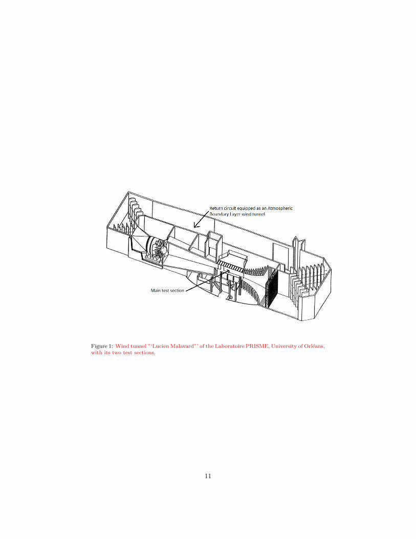
Figure 1: Wind tunnel ”‘Lucien Malavard”’ of the Laboratoire PRISME, University of Orleans,with its two test sections.

11

Figure 2: Modelled Atmospheric Boundary Layer properties. Vertical profiles of mean stream-wise velocity non-dimensioned with the mean streamwise velocity at hub height (left) andstreamwise, crosswise and vertical turbulence intensities (right).

12

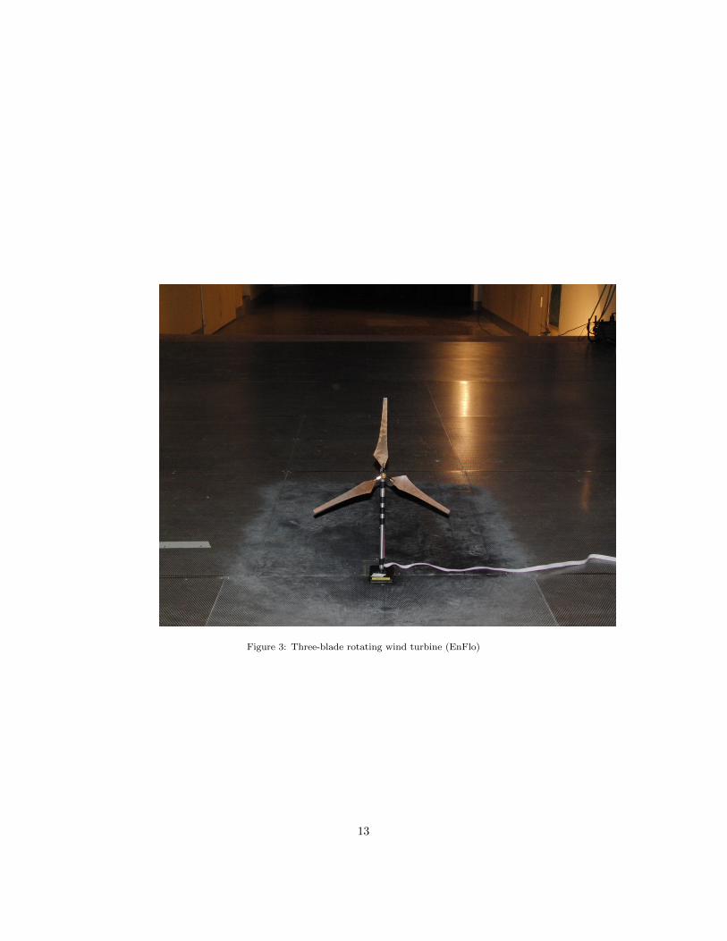
Figure 3: Three-blade rotating wind turbine (EnFlo)

13

Figure 4: Porous disc generating similar velocity deficit as the rotating wind turbine(PRISME)

14

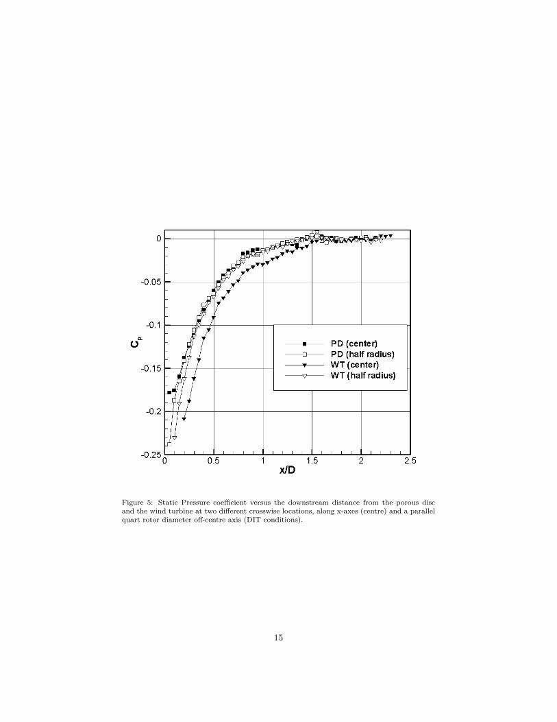
Figure 5: Static Pressure coefficient versus the downstream distance from the porous discand the wind turbine at two different crosswise locations, along x-axes (centre) and a parallelquart rotor diameter off-centre axis (DIT conditions).

15

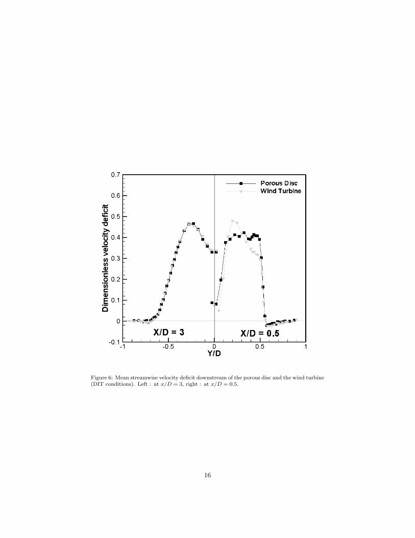
Figure 6: Mean streamwise velocity deficit downstream of the porous disc and the wind turbine(DIT conditions). Left : at x/D = 3, right : at x/D = 0.5.

16

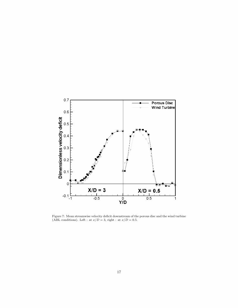
Figure 7: Mean streamwise velocity deficit downstream of the porous disc and the wind turbine(ABL conditions). Left : at x/D = 3, right : at x/D = 0.5.

17

Figure 8: Streamwise turbulence intensity downstream of the porous disc and the wind turbine(DIT conditions). Left : at x/D = 3, right : at x/D = 0.5.

18

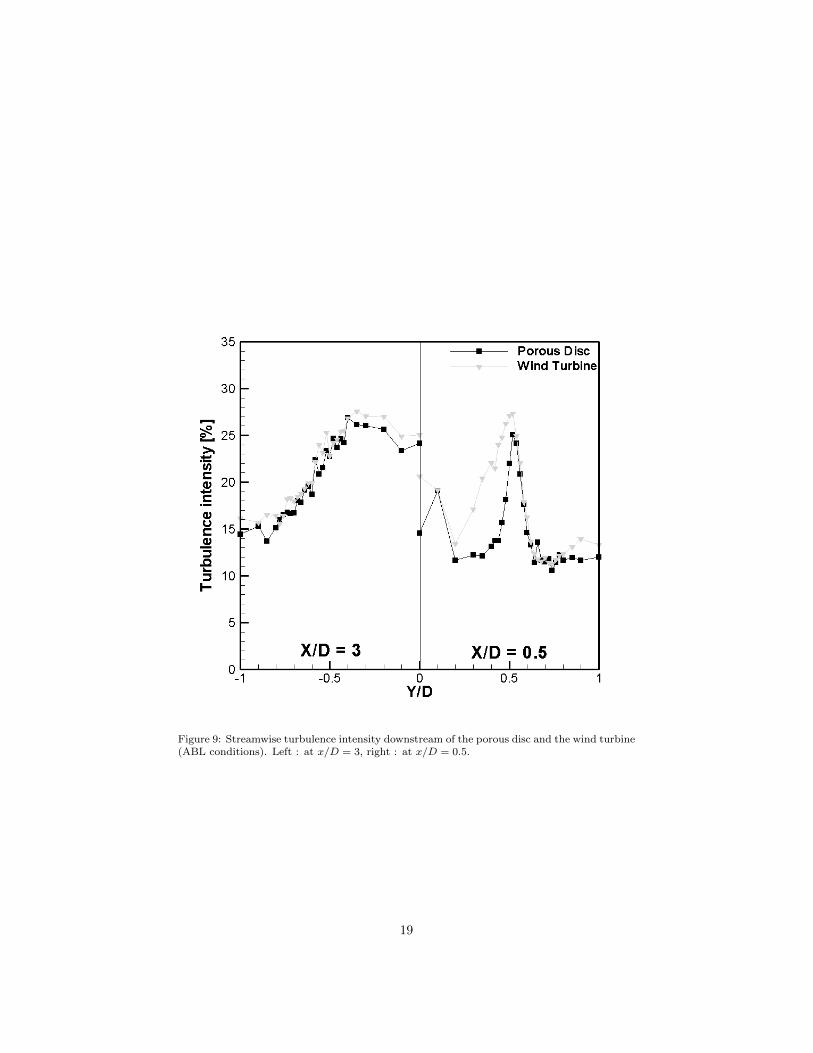
Figure 9: Streamwise turbulence intensity downstream of the porous disc and the wind turbine(ABL conditions). Left : at x/D = 3, right : at x/D = 0.5.

19

Figure 10: Streamwise skewness downstream of the porous disc and the wind turbine (DITconditions). Left : at x/D = 3, right : at x/D = 0.5.

20

Figure 11: Streamwise skewness downstream of the porous disc and the wind turbine (ABLconditions). Left : at x/D = 3, right : at x/D = 0.5.

21

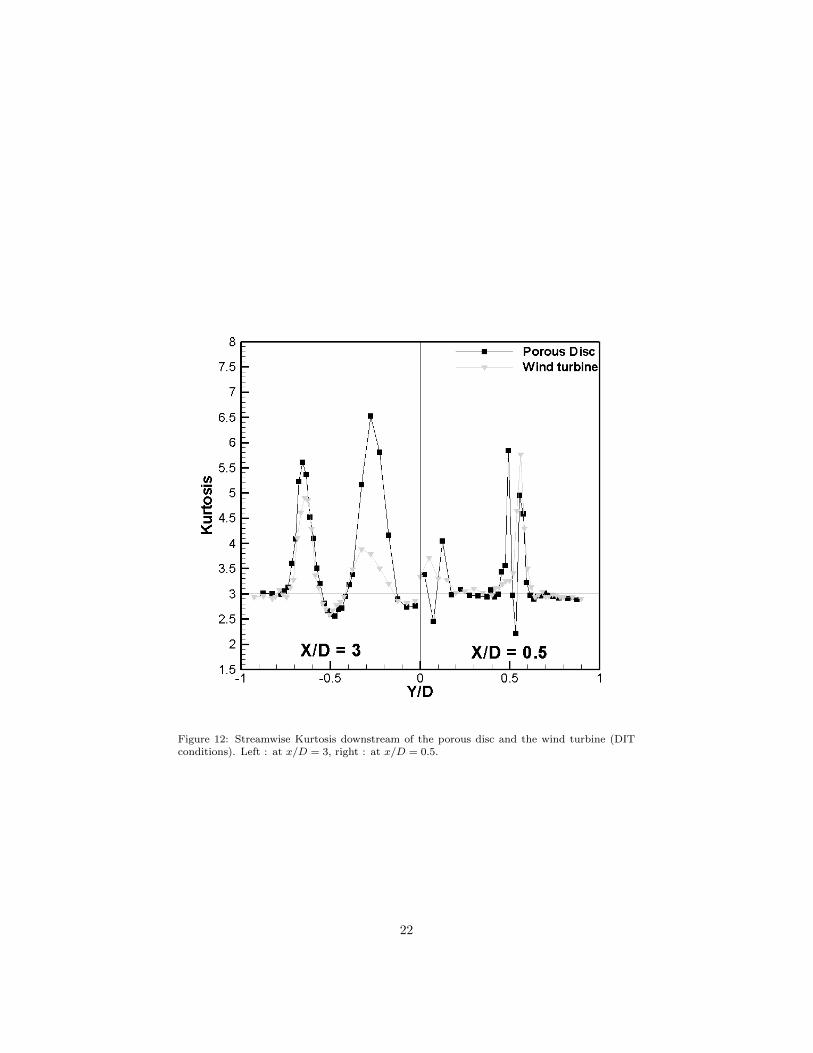
Figure 12: Streamwise Kurtosis downstream of the porous disc and the wind turbine (DITconditions). Left : at x/D = 3, right : at x/D = 0.5.

22

Figure 13: Streamwise Kurtosis downstream of the porous disc and the wind turbine (ABLconditions). Left : at x/D = 3, right : at x/D = 0.5.

23

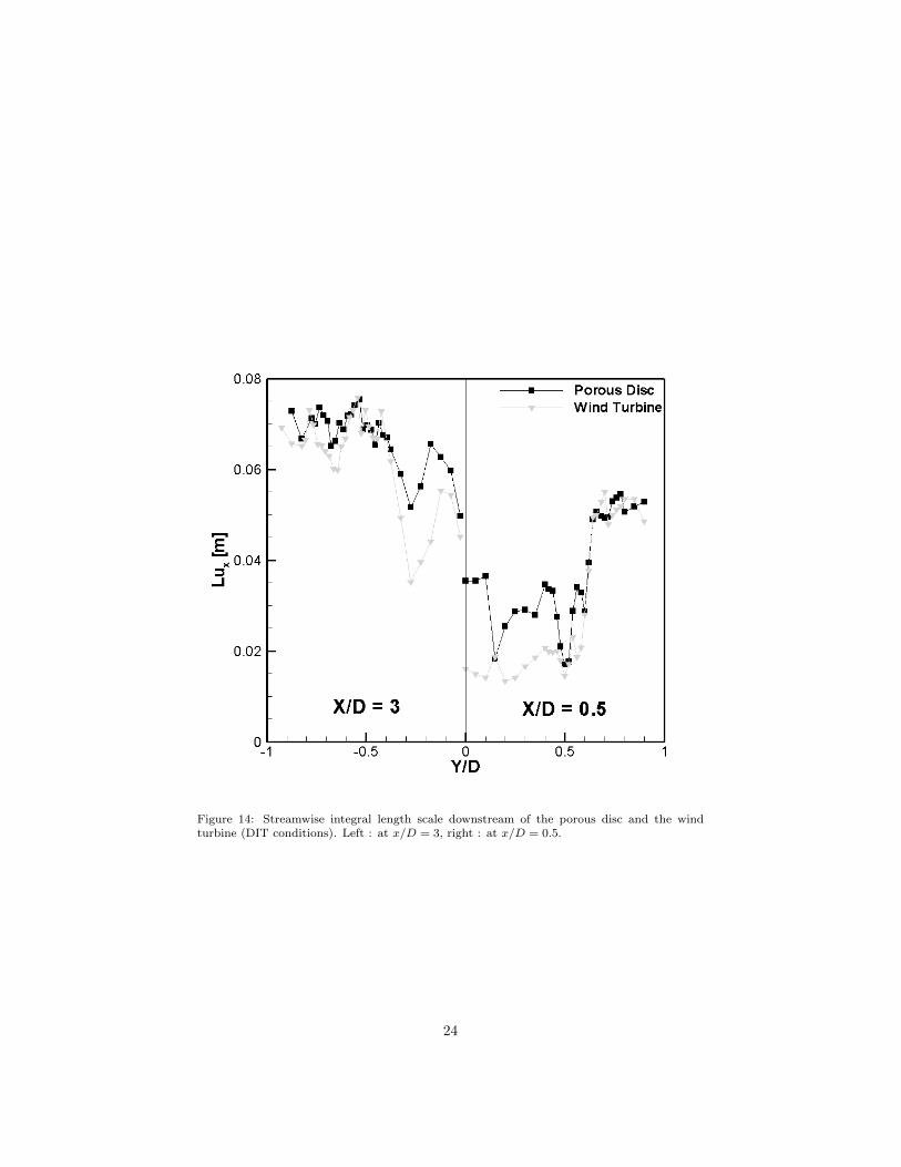
Figure 14: Streamwise integral length scale downstream of the porous disc and the windturbine (DIT conditions). Left : at x/D = 3, right : at x/D = 0.5.

24

Figure 15: Streamwise integral length scale downstream of the porous disc and the windturbine (ABL conditions). Left : at x/D = 3, right : at x/D = 0.5.

25

Figure 16: Spanwise profile of the mean vertical velocity downstream of the wind turbinemeasured at hub height. Left: in ABL inflow conditions (13% turbulence intensity at hubheight) , right: in DIT inflow conditions (4% turbulence intensity).

26

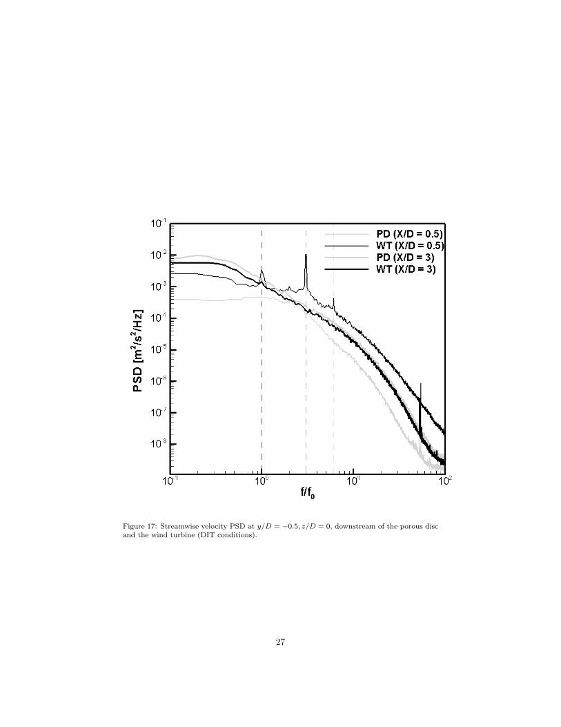
Figure 17: Streamwise velocity PSD at y/D = −0.5, z/D = 0, downstream of the porous discand the wind turbine (DIT conditions).

27

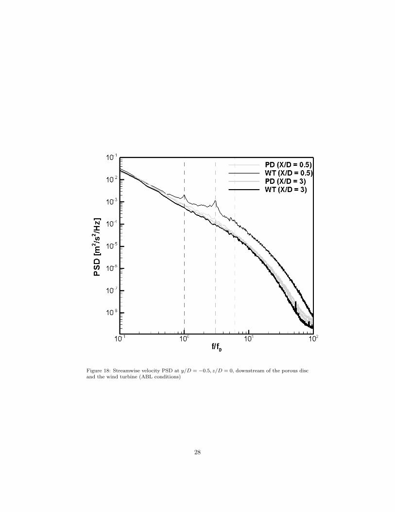
Figure 18: Streamwise velocity PSD at y/D = −0.5, z/D = 0, downstream of the porous discand the wind turbine (ABL conditions)

28