Featuring:• Using the Optimizer to Set Oscillator Frequency• The Fit to Standard Values Command• Fourier Analysis Guidelines

Applications for Micro-Cap™ Users

Winter 2016

The Optimizer

�

News In Preview

This newsletter's Q and A section describes several items: using the .IC command, model statement scope, old Micro-Cap executable versions, and MC8 workability on Windows 7 and 8. The Easily Overlooked Feature section describes the Build Command, a feature that makes building complex text commands easy.

The first article describes using Micro-Cap's optimizer to set a Wein Bridge oscillator's frequency and discusses some of the potential pitfalls.

The second article describes the Fit To Standard Values command, a convenient way of realizing un-usual resistor, inductor, or capacitor values from standard values.

The third article describes some suggestions for successful use of Fourier analysis.

Contents

News In Preview .................................................................................................................................................2Book Recommendations ....................................................................................................................................3Micro-Cap Questions and Answers .................................................................................................................4Easily Overlooked Features ...............................................................................................................................5Using the Optimizer to Set Oscillator Frequency ..........................................................................................6Fit to Standard Values Command ..................................................................................................................10Fourier Analysis Guidelines .............................................................................................................................15Product Sheet .....................................................................................................................................................21

�

Book Recommendations

General SPICE• Computer-Aided Circuit Analysis Using SPICE, Walter Banzhaf, Prentice Hall 1989. ISBN# 0-13-162579-9

• Macromodeling with SPICE, Connelly and Choi, Prentice Hall 1992. ISBN# 0-13-544941-3

• Inside SPICE-Overcoming the Obstacles of Circuit Simulation, Ron Kielkowski, McGraw-Hill, 1993. ISBN# 0-07-911525-X

• The SPICE Book, Andrei Vladimirescu, John Wiley & Sons, Inc., 1994. ISBN# 0-471-60926-9

MOSFET Modeling• MOSFET Models for SPICE Simulation, William Liu, Including BSIM3v3 and BSIM4, Wiley-Interscience, ISBN# 0-471-39697-4

Signal Integrity• Signal Integrity and Radiated Emission of High-Speed Digital Signals, Spartaco Caniggia, Francescaromana Maradei, A John Wiley and Sons, Ltd, First Edition, 2008 ISBN# 978-0-470-51166-4

Micro-Cap - Czech• Resime Elektronicke Obvody, Dalibor Biolek, BEN, First Edition, 2004. ISBN# 80-7300-125-X

Micro-Cap - German• Simulation elektronischer Schaltungen mit MICRO-CAP, Joachim Vester, Verlag Vieweg+Teubner, First Edition, 2010. ISBN# 978-3-8348-0402-0

Micro-Cap - Finnish• Elektroniikkasimulaattori, Timo Haiko, Werner Soderstrom Osakeyhtio, 2002. ISBN# 951-0-25672-2

Design• High Performance Audio Power Amplifiers, Ben Duncan, Newnes, 1996. ISBN# 0-7506-2629-1

• Microelectronic Circuits, Adel Sedra, Kenneth Smith, Fourth Edition, Oxford, 1998

High Power Electronics• Power Electronics, Mohan, Undeland, Robbins, Second Edition, 1995. ISBN# 0-471-58408-8

• Modern Power Electronics, Trzynadlowski, 1998. ISBN# 0-471-15303-6 Switched-Mode Power Supply Simulation • SMPS Simulation with SPICE 3, Steven M. Sandler, McGraw Hill, 1997. ISBN# 0-07-913227-8

• Switch-Mode Power Supplies Spice Simulations and Practical Designs, Christophe Basso, McGraw-Hill 2008. This book describes many of the SMPS models supplied with Micro-Cap.

�

Micro-Cap Questions and Answers

Question: Is there a way to use the state variable file *.TOP output from the transient analysis as the starting point for a DC temp sweep?

Answer: No. One other method is to run transient, do a DC OP only, then use the State Variables editor (F12) .IC command to create an .IC statement which then might later benefit DC analysis. Of course DC sweep involves stepping things which usually change the operating point rendering the initial conditions in the .IC statement obsolete. Still, the method may prove useful as a good initial guess for each step.

Question: If I have two subcircuits (or macros) that both contain a model statement of the same name, will that cause a conflict? If not which one will be used?

Answer: Each subcircuit uses the model statement within its .SUBCKT command or macro circuit. Each subcircuit is unaware of the other statement so there is no conflict. Another way of saying this is that the scope of each model statement is limited to the subcircuit (or macro).

Question: While tidying up I noticed that the MC11 directory has a lot of exe files etc. which seem to have accumulated with all the updates. Does MC11 need them all? I suspect some are there only for historical reasons.

Answer: When downloading a new executable from the Help / Check for Updates, the program makes a backup of earlier versions so that you can revert to them if desired. Most people never use these backups, so feel free to remove them if you wish. One caveat though, Spectrum does not provide backups of these earlier versions so if you ever want to use them you won't be able to once they are removed.

Question: I have a problem with my microcap 8. I try to install microcap 8 on my lap top, the secu-rity key don’t work, I connect it to the lap top but the program said key not found!

Answer: MC8 will not work in Windows 7 or 8 or 10 with a standalone key. It will only work on these operating systems if the key is a network key. If you have a network key, you should be able to install and run MC8 on Windows 7 or 8 or 10.

�

Build Command

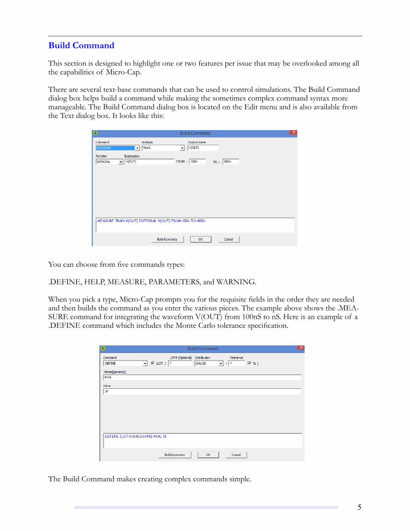
This section is designed to highlight one or two features per issue that may be overlooked among all the capabilities of Micro-Cap.

There are several text-base commands that can be used to control simulations. The Build Command dialog box helps build a command while making the sometimes complex command syntax more manageable. The Build Command dialog box is located on the Edit menu and is also available from the Text dialog box. It looks like this:

You can choose from five commands types:

.DEFINE, HELP, MEASURE, PARAMETERS, and WARNING.

When you pick a type, Micro-Cap prompts you for the requisite fields in the order they are needed and then builds the command as you enter the various pieces. The example above shows the .MEA-SURE command for integrating the waveform V(OUT) from 100nS to nS. Here is an example of a .DEFINE command which includes the Monte Carlo tolerance specification.

The Build Command makes creating complex commands simple.

�

Using the Optimizer to Set Oscillator Frequency

The optimizer can be used for many tasks, from optimizing a design to curve-fitting. One task that frequently comes up is oscillator frequency setting. This article will describe how to do that for a Wein-Bridge oscillator. Consider the circuit below.

Fig. 1 - Wein-Bridge oscillator

Fig. 2 - Transient analysis with oscillation at about 15KHz.

The circuit is set up to produce a sine wave of about 15KHz. Its transient run looks like this:

�

The plot has two objects that measure oscillation frequency. First there is a piece of formula text:

Measured oscillation frequency = Frequency(V(OUT),1,20) = [Frequency(V(OUT),1,20)]

This text uses a performance function to measure the frequency of oscillation. If you double click on the text (while in Select mode) you see its text dialog box.

Note that the Formula box is checked and that square brackets are used to delimit the formula. The actual function is:

Frequency(V(OUT),1,20)

This performance function measures the frequency of the waveform V(OUT), conditioned with a Boolean value of 1 (always true), with the measurement taken at the 20'th cycle to allow for some settling time.

Note that the delimiters tell the program where the formula is so that it can be distinguished from the remaining text.

There is another object in the plot, a Performance Tag. The tag's text looks like this:

Frequency(V(OUT),1,20)

The tag measures the same frequency that the text measures but places a set of arrows to indicate where it is making the measurement.

Fig. 3 - Formula text for measuring the frequency

�

To see the optimizer select it from the Transient menu, or press CTRL+F11. The dialog box looks like this:

Fig. 4 - The Optimizer dialog box

The optimizer is set up to find the value of the parameter C (which is C1's value) to equate the fre-quency to 10 KHz. It uses the same performance function used in the plot:

Frequency(V(OUT),1,20)

Press F2 to start the optimizer. After a few seconds the screen looks like this:

Fig. 5 - The Optimizer result

�

The optimizer has calculated 1.58196nF for the C1 value needed to produce a frequency of 10KHz.As it stands, the value of C1 is unchanged. If you want to use the optimized value in the circuit you can do so by pressing the Apply button. Do that now and then press the Close button.

Now press F2 to run the analysis using the optimized value. The plot should look like this:

Fig. 6 - Transient analysis with oscillation at 10KHz.

As you can see the measured frequency is 10K as specified. Notice that the theoretical frequency for the optimized value of C1 is 1/(2*PI*R* 1.581961n) = 10.061K but the actual measured frequency is 10.0K. The theoretical frequency formula assumes an ideal gain element.

Several things to keep in mind:

Test the circuit with your performance function before optimizing: Use a range of C1 and Maximum Time Range values to be sure that the optimizer can actually find a useful frequency. For instance, if you had used a TMAX of 1ms the optimizer would fail because it would not have found a 20'th cycle to measure.

Use an adequate Maximum Time Step: If the time step is too large the optimizer may find an inaccurate value. How can you tell? One way is to run with formula text (or if you have MC11, the Measurements window) measuring frequency, trying different timesteps. Keep increasing the Maxi-mum Time Step until you see a significant change in the measured frequency. Use the largest value you can to minimize optimization run time. If the timestep is too large you get inaccurate measure-ments. If it's too small the runs take too long.

10

Using the Fit to Standard Values Command

Did you ever create a circuit with non-standard resistor or capacitor values and wonder how you'd build it? Use the Fit to Standard Values Command. It builds the component value by constructing it from a combination of standard parts or, if desired, it will use the single nearest standard value. To illustrate we'll use the same Wein-Bridge oscillator circuit used in the last article.

Fig. 7 - Wein-Bridge oscillator

This circuit has mostly standard values except for two. R3 and R4 are not standard values. We'll use the command to construct them. The command can be found on the ever useful Change dialog box, at Edit menu / Change / Fit to Standard Values. It looks like this:

This command either fits all selected components to single standard values or constructs them from series and parallel combinations. Click on the Preferences Combinations... to view the options. It looks like this:

Fig. 8 - Fit to Standard Values dialog box

11

This dialog lets you select the maximum error, the maximum part count, the maximum number of series elements to use, and the name of the file containing standard parts, when building the value from combinations.

Go back to the schematic and press CTRL+A to select all parts. Then select the Fit to Standard Values command. Click OK and you'll see the schematic but with a new Page Tab called Standard Values. Click on it and you'll see a report detailing how each value was achieved.

*********************************************** Fit To Standard Values Command Results ** Method = Combinations ** Matched parts = 8 ** Total parts required = 11 ** Largest matching error = 0% ***********************************************Parts=RB1,RF1,R2,R1File = C:\MC11W\library\standard.resOriginal Value = 10KCombinations Value = 10KPercent Error = 0Number of parts needed = 110K = 10K

Part=R3File = C:\MC11W\library\standard.resOriginal Value = 12KCombinations Value = 12KPercent Error = 0

Fig. 9 - The Fit Options

1�

Number of parts needed = 212K = (21K | 28K)

Part=R4File = C:\MC11W\library\standard.resOriginal Value = 24KCombinations Value = 24KPercent Error = 0Number of parts needed = 324K = 23.7K+(2.55K | 340)

Parts=C1,C2File = C:\MC11W\library\standard.capOriginal Value = 1nCombinations Value = 1nPercent Error = 0Number of parts needed = 11n = 1n

Resistor part count:10K 421K 128K 123.7K 12.55K 1340 1Total 9

Capacitor part count:1n

All parts except the R3 and R4 were obtained from standard values. The R3 resistor was constructed as follows:

12K = (21K | 28K)

This syntax means the 12K was constructed from a 21K in parallel with a 28K, both standard values.

The R4 resistor was built as follows:

24K = 23.7K+(2.55K | 340)

This syntax means the 24K was constructed from a 23.7K in series with a parallel combination of a 2.55K and a 340, both standard values.

The largest matching error was zero.

The Fit to Standard Values command is a very handy way to realize unusual values of resistors, ca-pacitors, and inductors.

1�

Here is another circuit to illustrate.

From the schematic, press CTRL+A to select all parts. Then select the Fit to Standard Values com-mand. Click OK and you'll see the schematic modified to look like this:

Fig. 10 - Another sample circuit

Fig. 11 Sample circuit modified by Fit to Standard Values Command

Click on the Standard Values tab of the schematic to see how these values were arrived at.

1�

*********************************************** Fit To Standard Values Command Results ** Method = Combinations ** Matched parts = 2 ** Total parts required = 4 ** Largest matching error = -0.18% ***********************************************Part=R1File = C:\MC11W\library\standard.resOriginal Value = 18652Combinations Value = 18.664KPercent Error = 0.064Number of parts needed = 218.664K = 18.2K+464

Part=R2File = C:\MC11W\library\standard.resOriginal Value = 4432Combinations Value = 4.424KPercent Error = -0.18Number of parts needed = 24.424K = (28.7K | 5.23K)

Resistor part count:18.2K 1464 128.7K 15.23K 1Total 4 R1's desired resistance of 18652 was approximated by 18664. It was implemented with a series com-bination of an 18.2K and a 464, for an error of 0.064%

R2's desired resistance of 4432 was approximated by 4424. It was implemented with a parallel com-bination of an 28.7K and a 5.23K, for an error of -0.18%.

These are typical numbers for the command.

The command can be accessed globally as we've described here and also when the parts are entered from the Attribute dialog box.

1�

Fourier Analysis Guidelines

Fourier analysis is an important adjunct to transient analysis. Used properly, it can provide invaluable information about the frequency content of transient waveforms. But how do you use it properly? Here are some guidelines:

1) Make sure that the FFT fundamental frequency matches the lowest frequency of all sources in the circuit. If you have more than one source, examine each and determine its frequen-cy. Then take the lowest frequency and make sure it matches the computed Frequency Step at:

Properties Menu (F10) / Fourier / Frequency Step

The Frequency Step is computed as follows:

1 / (Upper Time Limit - Lower Time Limit)

The Upper Time Limit should nearly always be TMAX from the transient analysis Time Range.

The Lower Time Limit defaults to TSTART which is usually zero. It is the point at which data col-lection begins (all other plot data prior to that is discarded).

2) Simulate long enough to get past the initial transients. Transients make the waveform aperi-odic tainting the FFT results. There are two useful options here:

a) Use Periodic Steady State (PSS) b) Use a long run and exclude the transient-tainted front part.

Always use PSS if it is available. PSS is only available from MC10 on. Also, PSS does not work with circuits containing transmission lines, digital parts, Laplace sources, Z-transform sources, or N-ports, and PSS sometimes fails to converge. In that case you use option b.

Set the Time Range long enough to minimize transients and still leave enough time at the end to cover the FFT fundamental period. By making the Lower Time Limit greater than zero, you can remove transient portions of the waveform, making it more periodic.

3) Use a small enough timestep to get an accurate waveform. For ordinary work, make the Maximum Time Step, DTMAX = TMAX / 100. For higher precision use DTMAX = TMAX / 1000. Using a smaller DTMAX will produce an improvement in the accuracy of the smaller har-monics.

4) To increase the frequency resolution make the time range longer. Since the Frequency Step is:

1 / (Upper Time Limit - Lower Time Limit)

increasing the value of Upper Time Limit makes the frequency step providing more resolution. If you do this, don’t forget to increase the number of harmonics to auto scale to compensate in the FFT plot.

1�

So let's see how this works in an actual example. Consider this circuit:

This circuit has two sine wave sources, V1 at 2MHz and V2 at 1MHz. So immediately we know the FFT will have important frequency content at these frequencies and we know that the FFT Frequency Step value must be no larger than 1MHz. Select transient analysis, then select Transient menu / Fourier Windows / Add Fourier Window. It has already selected the dB(Harm(V(OUT))) for the plot. Select the Fourier tab. It looks like this:

This is the Fourier panel for the Fourier Properties dialog box. There is a similar dialog box and pan-el for the Properties for Transient Analysis. To access the Properties dialog box, use F10 from either the Fourier window or the transient analysis plot. The important fields of this window are these:

Upper Time Limit: This sets the upper time limit for FFT functions. Generally this is set to a mul-tiple of the fundamental period, typically 3-5 periods.

Lower Time Limit: This sets the lower time limit for FFT functions. This is set to a multiple of the fundamental period to avoid startup transients in the target waveform and is typically 2 - 4 periods.

Fig. 12 Sample circuit for Fourier analysis

Fig. 13 Fourier panel for the Fourier window

1�

If PSS is used, and it usually should be, you can employ one period.

Frequency Step: This is the fundamental frequency computed from the difference in the upper and lower time limits. If you enter a value, then MC11 computes a compatible value for the lower time limit. The formula used is:

Frequency Step = 1 / (Upper Time Limit - Lower Time Limit)

You can also use these variables in the time limit fields:

TMAX Maximum run time of the transient analysisTSTART Time when data collection starts typically 0

For example, you might use TMAX as the entry in the Upper Time Limit field and TSTART or (to exclude startup transients) perhaps 0.5*TMAX as the entry for the Lower Time Limit field.

Number of Points: This sets the number of interpolated data points to use for FFT functions. Typi-cally 1024, 2048, or 4096 are nearly always suitable choices.

Auto Scaling: This group controls auto scaling options and includes these options:

Include DC Harmonic: This option includes the DC harmonic when auto scaling is done. Typically it is disabled.

Auto Scale First .... Harmonics: This number specifies the number of harmonics to include when auto scaling.

Press F2 to start the run and the screen should look like this:

Fig. 14 Fourier window and transient plots for plot first 10 harmonics

1�

The first thing you notice is that we barely get the 1MHz in the plot. That's because the Number of Harmonics to include in auto scaling is 10 and the frequency is computed as,

Frequency Step = 1 / (10uS - 0) = 100KHz

Click on the Fourier window, then press F10. Select the Fourier tab and change the Auto Scale First value from 10 to 50. Press F2 to start the run and you should see this:

Now we can clearly see the 1MHz and 2MHz values. There is a significant amount of aliasing due to the initial transients which causes the waveform to be non-periodic. Let's fix that with PSS. Press F9 and enable Periodic Steady State. Press F2 to start the run. You should see this:

Fig. 15 Fourier window and transient plots for plot first 50 harmonics

Fig. 16 Fourier window and transient plot using PSS

1�

Notice now that the noise floor is about 170 dB versus 50dB before. Suppose we couldn't use PSS. What then? Well we can use a tighter lower window limit to eliminate much of the transient. Press F9 and disable Periodic Steady State. Click on the Fourier window, then press F10. Select the Fourier tab and change the Lower Time Limit to TMAX/2. Notice that this changes the Frequency Step to 200KHz. Press F2 to start the run and you should see this:

The noise floor now is about 100 dB. Better than the original 50dB, but not as good as PSS. How about increasing the frequency resolution? Here's how to do that. Press F9, change the Time Range to 50u. Click on the Fourier window, then press F10. Select the Fourier tab and change the Baseline to -400 and change Auto Scale First to 200 harmonics. Press OK then F2 to start the run. It should look like this:

Fig. 17 Fourier window and transient plot using the lower time limit to minimize transients

Fig. 18 Fourier window and transient plot using the lower time limit to minimize transients

�0

Things to Watch Out For

There are two Properties dialog boxes: one for transient plots and one for Fourier Windows.

When a transient analysis is complete, the focus is sent to the analysis plot, so pressing F10 to see the Properties dialog will invoke the Properties for Transient Analysis. Any changes made here in the Fourier tab will affect only the transient analysis plot.

To display the Properties for Fourier, first click in the Fourier window and then press F10. Any changes made here in the Fourier tab will affect only Fourier Windows.

�1

Product Sheet

Latest Version numbersMicro-Cap 10 .......................................................................Version 11.0.1.6Micro-Cap 10 .......................................................................Version 10.1.0.5Micro-Cap 9 .........................................................................Version 9.0.9.1Micro-Cap 8 .........................................................................Version 8.1.4.0Micro-Cap 7 .........................................................................Version 7.2.4

Spectrum’s numbersSales .......................................................................................(408) 738-4387Technical Support ...............................................................(408) 738-4389FAX ......................................................................................(408) 738-4702Email sales ............................................................................sales@spectrum-soft.comEmail support ......................................................................support@spectrum-soft.comWeb Site ................................................................................http://www.spectrum-soft.com