wireless service pricing under multiple competitive providers and

0

Wireless Service Pricing under MultipleCompetitive Providers and Congestion-sensitive

Users

Andre Nel and Hailing ZhuUniversity of Johannesburg

South Africa

1. Introduction

With the deregulation of telecommunication industry and the fast development of broadbandwireless technologies, i.e., Wireless Mesh Network (WMN), WiFi (802.11g) and WiMAX(802.16), it can be imagined that in the future users can access Internet or other wirelessservices, e.g., telephony, through diverse wireless service providers (WSPs) and technologies.In this complex networking landscape, moving decision-making from access points to usersis a path to achieving system scalability (Zemlianov & de Veciana, 2005). Thus, for users,it is increasingly the case that they have more freedom to choose among several WSPs whoprovide wireless services instead of being contractually tied to a single WSP. For example,a user wishing to access the Internet via a WiFi hotspot or access point (AP) may find himin a zone covered by several wireless access providers, or he may choose among differenttransmission platforms: WiFi, WiMAX, 3G, and so on. In such a market, in which multipleWSPs compete for users who are price- and congestion-sensitive, it is important to investigatethe economic issues that arise due to the presence of multiple competing service providers.In such a competitive environment, all players are self-interested in a sense that their actionsor reactions in response to others’ actions only focus on maximizing their own payoffs. Froma WSP’s point of view, it has to compete for users with other WSPs while maximizing itsprofit. From a user’s point of view, he aims to maximize his compensated utility by choosinga WSP offering the best trade-off between quality of service (QoS) and price. Our primarygoal is to understand how each WSP sets its price in the presence of price-sensitive andcongestion-sensitive users and other competing WSPs to maximize its own profit. Note thatwe focus on the price setting problem among multiple WSPs instead of price discriminationamong users. Thus we simply assume that the users are homogeneous in utility functions andwillingness to pay.According to the current design of WMN architectures, a user’s requests will be routed to oneAP or base station (BS) (in the IEEE802.16 standards APs of the IEEE 802.11 are called basestations) automatically so that the data flows generated by the user’s requests can take themost appropriate route in terms minimum hop count or other QoS metrics (i.e., bandwidth,end-to-end delay, and so on). However, from the user’s point of view, besides QoS, the priceis also an important consideration when the user selects an AP or BS for wireless servicedelivery. It is generally accepted that the current wireless data network models are flawed inthe sense that they fail to capture (Das et al., 2004):

12

www.intechopen.com

2 Wireless Mesh Networks

– The utility of the services and network from the user’s perspective;

– The impact of user demands on revenue utility from the service providers perspective.

Even though the current design of architectures, algorithms and protocols for WMNs doestake users’ QoS requirement into account, price competition among WSPs is not taken intoconsideration. We believe that in the presence of competition among multiple WSPs withdifferent prices resource distributions within the network would be affected significantly. Thiswould in turn affect the engineering design of WMNs and other wireless delivery models. Inour pricing model, we assume that users can choose a WSP’s AP or BS based on the WSPs’quoted prices and the perceived QoS instead of just being directed automatically to a certainAP or BS by routing protocols.In order to obtain a return on investment, each service provider needs a pricing strategy tocharge its users for the service it offers. Pricing communication network services has beenseen as a soft tool to cope with congestion, to control demand, and to induce users to usethe network in a desirable way while maximizing service providers’ profits. A well-designeddynamic pricing policy allows a service provider to capture the changes of users behaviorand network status, and to adjust its prices based on these dynamic changes. In the caseof high network utilization, the service provider increases its price, which in turn makesprice-sensitive users reduce their demand as a response. Similarly, in the case of low networkutilization, the service provider decreases its price to attract more users. With a proper pricingscheme, a service provider and its users are allowed to act individually to express the valuesthat they are willing to charge or pay, and to reach an equilibrium where their individualutilities are maximized simultaneously. Furthermore, in the presence of other competingservice providers, each WSP’s price is dependent on other service providers’ prices andnetwork status, which affect users behavior because utility maximizing users always choosethe service provider offering the best combination of price and QoS.Game theory attempts to model the strategic interactions among self-interested playerswho must make choices that potentially affect other players’ interests. In particular,non-cooperative game theory is primarily used as a typical modeling tool to analyze situationsin which players’ payoffs depend on the actions of other players. In principle, in anon-cooperative game each player makes his decision independently and attempts to get themost out of the game on the basis that the other player is not cooperating in any way. In thischapter, we discuss an oligopoly, in which multiple WSPs with asymmetric costs providingwireless services with possibly different qualities compete for a group of users through theirprices, using a game-theoretical approach. Our objective is to develop a framework to analyzethe interaction among multiple competing WSPs and price- and congestion-sensitive usersand identify the Nash equilibrium prices.

2. Game theory for oligopoly and its applications to communication network

pricing

Game theory aims at modeling situations in which players have to make specific moves1 thathave mutual, possibly conflicting, consequences. In particular, it studies interactions amongself-interested players in a way that interaction strategies can be designed to maximize thepayoff of a player in a multi-player game. It also enable the development of mechanisms thathave certain desirable properties. As its name suggests, the basic concepts of game theory

1In the game theory terminology, a move constitutes taking a decision that will have pre-determinedconsequences.


www.intechopen.com

Wireless Service Pricing under MultipleCompetitive Providers and Congestion-sensitive Users 3

arose from the study of games such as chess and checkers (Parsons et al., 2002). However,it rapidly became clear that the techniques and results of game theory can be applied to allinteractions that occur between self-interested players. The classic game theoretic questionasked is: what is the best or the most rational thing a player can do? In most multi-playergames, the overall outcome depends critically on the choices made by all players involved.This implies that in order for a player to make a choice that optimizes his payoff, he mustreason strategically. That is, the player must take into account the decisions that otherplayers may make, and must assume that they will act rationally so as to optimize their ownpayoffs. Game theory provides a mathematical framework for formalizing and analyzingthese situations and finding the possible results of the games.Emerging as a tool for modeling and solving economic problems, game theory has alsofound its way into other domains where conflicting multiple parties have conflicting goals.Naturally, it has been used extensively for studying pricing problems for the Internet, ormore generally telecommunication networks, e.g. (Altman & Basar, 1998) (La & Anantharam,1999) (Altman et al., 2006) (Musacchio & Walrand, 2006). In Internet pricing, the fundamentalaspects of multi-party (Internet service providers (ISPs) and users) optimization problems canbe captured by game theory. The outcomes of a game are the utilities of every players. TheISPs and the users respectively choose their best strategies (the price for the ISPs and thedemand for the users for instance) to get their desired outcomes.Normally, pricing with a game theoretic approach is related to network resource managementproblem. Cooperative game theory, which requires signalization or agreements among player,has been used to obtain a Nash bargaining framework to address network issues like resourceallocation, network efficiency, fairness and at the same time service provider’s revenuemaximization and pricing (Yaıche et al., 2000). In (Dziong & Mason, 1996), it is shown thatthe cooperation between two ISPs benefits both the ISPs and the users. In (La & Anantharam,2002), La et al. propose an algorithm in which the network providers adjust their pricesand the users adjust their rates so that an optimal equilibrium is reached, while maintainingproportional fairness.However, in a wireless service competition market with multiple competing WSPs and aset of users, all players have conflicting interests. On one hand, the WSPs’ ultimate goalis to maximize their own revenues. Their attempt to maximize user’s satisfaction, systemutilization, etc., is merely an approach to achieve this ultimate goal. Hence, in this WSPsand users game, the revenue is modeled as the WSP’s payoff. On the other hand, users wantto maximize their own satisfaction with minimum expense, given that they have freedom tochoose their WSPs and switch from one WSP to another. Then the user’s overall satisfaction ismodeled as user payoff. Since these two goals are different and even conflict with each other,there is no apparent motivation for WSPs and users to cooperate with each other to achieve asingle optimal goal as suggested by cooperative game theory2.In contrast to cooperative game theory, non-cooperative game theory is concerned withsituations in which players’ payoffs (utilities) depend on the actions of other players and inwhich the players cannot, in principle, sign binding agreements enforceable by third parties.The following sections give a brief introduction to the theory of non-cooperative games andits applications in Internet price competition games.

2Given that cooperation by the WSPs is incompatible with most regulatory frameworks, the interactionamong the WSPs can also not be modeled by cooperative game theory.

283Wireless Service Pricing under Multiple Competitive Providers and Congestion-sensitive Users

www.intechopen.com


2.1 Non-cooperative games in strategic form and nash equilibrium

Non-cooperative game theory is a powerful tool for solving problems with conflicting goals.In a non-cooperative game, there are a number of players who have potentially conflictinginterests, where each player has a set of strategies with associated payoff values, and makeshis decision independently and attempts to obtain the best payoff without cooperating anyplayer in any way. The outcome of the game is a set of strategies, each coming from thestrategy set of an individual player, that optimizes the payoffs of all players. In the context ofwireless data networks, the player are the WSPs and users. In compliance with the practice ofgame theory, we assume that both WSPs and users, are rational, meaning that their objectivesare to maximize their payoffs (or utilities) individually.Basically, there are two types of representations generally used to represent a game. Strategicform (or normal form) is the basic type used in studying non-cooperative games. Normally,strategic form games deal with the situation where the strategy decision of each player is madeat the same time without observing the decision of the other player. On the other hand, theextensive form (also called a game tree) is a description of how a game is played over time. It isgenerally assumed that a single player can move based on observation of the prior choices ofother players when the game is at a given stage. Generally speaking, games in extensive formdeal with the situation where at least one player has partial information about other players’decision. There are two different scenarios for an extensive form game: a game of completeinformation is the strategic interaction when players are aware of each other’s strategies orpayoffs, i.e., all factors are common knowledge. In the game of incomplete information, atleast one player is unaware of the payoffs or strategies of the other player.In today’s competitive communication market, it is impossible for service providers todivulge their payoffs or strategies to their rivals. In this chapter, all WSPs simultaneouslyand independently compute their quoted prices without the knowledge of their opponents’payoffs or strategies. Each WSP sets its own prices based on the users’ response, but has noknowledge about other WSPs’ prices and the users’ response to other WSPs’ prices in realtime. Clearly, in this pricing game among multiple competing WSPs, the users’ reaction tothe WSPs’ quoting prices and QoS is the determining factor. Therefore, this price competitiongame can be divided into two games:

– a game between the WSPs and users which can be expressed as a leader-follower game instrategic form with the users as the follower responding to the WSPs’ prices and QoS; and

– a game among the WSPs which can be expressed as a simultaneous move game in strategicform.

A game in strategic form can be defined as G = (i ∈ N,Si,Ui), where N is the set of players,each of whom attempts to maximize his own particular utility. Si represents the strategyspace of player i, which is the set of all possible strategies of player i. A joint set of the strategyspaces of all players constitutes a strategy profile s = {s1, s2, . . . , sN}. ui(s) is payoff or utilitythat quantifies the outcome of game for player i given the strategy profile s. Fig. 1 illustrates asimplest example of two-player strategic form game with each player having two strategies.In our case the players are a set of WSPs whose strategy and payoff are price and profit,respectively, and a group of homogeneous users who need to decide to choose which WSP tosubmit their requests based on the combination of the WSPs’ offered prices and correspondingQoS, which are factors of user’s utility function. Note that we have assumed that the users arehomogeneous in utility function in the introduction to this chapter. We further assume thatthe profit function are the same for all WSPs.


www.intechopen.com


Player1

Player2s22

s12

Strategy

Strategy

u1({s11, s21}), u2({s11, s21})s11

s21

u1({s12, s21}), u2({s12, s21}) u1({s12, s22}), u2({s12, s22})

u1({s11, s22}), u2({s11, s22})Strategy

Fig. 1. A two-player game in strategic form.

To solve the game, the concept of best response needs to be introduced first. The best response

of player i to the profile of strategies of other players is a strategies s′i such that

ui(s′i, s−i) > ui(si, s−i) ∀s−i ∈ S−i, (1)

where subscript −i represents all the players except player i himself. If all players’strategies are mutual best responses to each other, then no player would have a reason todeviate from the given strategy profile. The situation in which no players has incentive tounilaterally changing his current strategy is called a Nash equilibrium. Mathematically, aNash equilibrium is a strategy profile s∗ = {s∗1 , s∗2 . . . , s∗N} such that for each player i

ui(s∗i , s−i∗ ) ≥ ui(si, s

∗−i) ∀si ∈ Si. (2)

In a Nash equilibrium, none of the players can gain by unilateral deviation, which implies thatno single player can leave this point without the cooperation of others in order to improve hisown utility. In other words, a Nash equilibrium is a strategy profile comprised of mutual bestresponses of all the players3.

2.2 Price and QoS competition in telecommunication networks

Pricing has been seen as a soft tool to control demand, to cope with congestion and to dealwith heterogeneous applications with different QoS requirements. Therefore, there has beenan increased research interest in telecommunication network pricing, which leads to manyproposals for new pricing schemes motivated by different objectives, e.g. to allocate scarcenetwork resources efficiently in order to maximize social welfare, i.e. (Kelly et al., 1998)(Low & Lapsley, 1999) (Yaıche et al., 2000) (Tassiulas et al., 2001) (La & Anantharam, 2002)(Shu & Varaiya, 2003) (Qiu & Marbach, 2003), to maximize service provider’s revenue, i.e.(Basar & Srikant, 2002) (M. Bouhtou & Wynter, 2003), to guarantee fairness among users,i.e. (Kelly et al., 1998) (Kelly, 2000), to satisfy QoS requirements for differentiated networkservices (La & Anantharam, 1999) (Wang & Schulzrinne, 1999) (Mandjes, 2003). With therapid growth of wireless data networks, e.g. wireless ad hoc networks and wireless meshnetworks, recently many price-based resource allocation schemes also have been propose forwireless data networks, i.e. (Xue et al., 2003) (Das et al., 2004) (Xue et al., 2006) (Luthi et al.,2006) (Kao & Huan, 2008). Pricing has also been used as an incentive mechanism to stimulateparticipation and collaboration of self-interested wireless node in wireless mesh networks, i.e.(Lam et al., 2006) (Lam et al., 2007).A very large proportion of these proposed pricing schemes focus on the monopolistic case,where there is only one service provider dealing with a multitude of users and the the

3It should be noted that even though the Nash equilibrium indicates an equilibrium solution it maynot be a solution that maximize the social welfare.


www.intechopen.com


service provider is big enough to affect the entire market. However, as telecommunicationnetworks have progressively switched from a monopolistic network to a oligopolistic onewith competitive service providers, more attention has been given to price competition amongservice providers, see for example, (Gibbens et al., 2000) (Cao et al., 2002) (Sakurai et al., 2003)(Armony & Haviv, 2003) (Ros & Tuffin, 2004) (Khan, 2005) (Zhang et al., 2008).In practice, markets are often partly regulated and partly competitive. In the rest of thischapter, we only discuss pricing game under perfect competition in a market withoutregulation, in which all service providers have certain market force and there is no providerso dominant that one of them can control the price. Therefore, no one is the leader and noone is the follower in such a price competition game. As a consequence, all service providers’prices are determined by the market in which users have the ability to switch from one serviceprovider to another. The basic assumptions of the price competition game are that both serviceproviders play the role of rational decision makers and each service provider knows that theopponents are also rational. A rational service provider always attempts to select the bestresponse strategy.In the rest of this section we will introduce some proposed pricing schemes reported inliterature, which are related the pricing model presented in the next sections.In (Gibbens et al., 2000), Gibbens et al. develop a framework to analyze competition betweentwo ISPs, either or both of which may choose to offer multiple service classes. In theiranalytic framework, there are two ISPs: ISP1 and ISP2 charging prices p1 and p2 per unittime respectively. On joining ISPi, a user receives utility Ui(θ) per unit time. Utility Ui(θ)has three components: a positive benefit V which is independent of which ISP he/she joins; adis-benefit which is a function of the degree of congestion on the network of the ISPi Ki andthe user’s preference for congestion θ; and a dis-benefit from having to pay a price pi per unittime to ISPi for its service. To describe the range of preferences in the population of users inthe simplest manner, assume that there is a continuum of users whose θ parameters form apopulation distribution which is uniformly distributed on the interval [0,1]. Thus the utilityof a user with preference θ from joining ISPi is defined as

Ui(θ) = V − θKi − pi (3)

For analytical simplicity, congestion on a network is defined as the number of users, Qi,

divided by the capacity of the network, Ci: Ki =QiCi

. Based on these assumptions, Gibbens

et al. analyze the duopoly price competition for packet-based networks and show that theunique equilibrium outcome for both networks is to offer a single service class and charge thesame price.Sakurai et al. (Sakurai et al., 2003) propose an extended model based on Gibbens et al.’s gametheoretic model for the case in which an opt-out strategy is introduced for users. In theirmodel, the users have three strategy options: joining one of the ISPs and opting out of bothof them. In (Sakurai et al., 2003) it is assumed that ISP1’s price is higher than ISP2’s price,p1 > p2, and both ISPs have the same fixed capacities C1 = C2 = C. A strategy for a user is achoice of ISP to join or opting out of both ISPs, given the prices quoted by the ISPs. If the user isindifferent between the two ISPs, his choice can be made randomly. Sakurai et al. suggest onlythe users who don’t like congestion nor higher price opt out of ISP1, or mathematically onlythe users whose utility U1(θ)< 0 (0 ≤ θ ≤ 1) choose opting-out. Therefore, there are two typesof marginal users as shown in Fig. 2: one is the users with congestion preference θ21, whoare indifferent between joining ISP2’s lower priced network and joining ISP1’s higher pricednetwork; and the other one is the users with congestion preference θ10, who are indifferent


www.intechopen.com


0 θ21 θ10 1

ISP2 ISP1 opt-out

θ

Fig. 2. Critical values of θ21 and θ10 for user preference (Sakurai et al., 2003)

between joining ISP1’s higher priced network and opting out of ISP1. If there are N usersin the market, the numbers of users who join ISP1 and ISP2 are given by Q1 = N(θ10 − θ21)and Q2 = Nθ21 respectively, provided that 0 < θ21 < θ10. Sakurai et al. conclude that Nashequilibrium for this non-cooperative game model greatly depends on three factors: the user’sbenefit from using the Internet, V, ISP’s network capacity, C, and the number of users inmarket, N.Notice that the fundamental of both models presented by Gibbens et al. and Sakurai et al. isto find the critical values of θ∗ determined by the indifference relation U1(θ

∗) = U2(θ∗). The

philosophy behind this is that when the user’s utilities for joining either ISP are equal twoISPs can reach a Nash equilibrium, in which each ISP’s pricing strategy is optimal in the sensethat one ISP has no incentive to change its price strategy in response to the other ISP’s strategyand vice versa. Because the users are indifferent between joining ISP1 or joining ISP2 whenthe utilities for joining either ISP are the same, no user of one ISP has an incentive to switchto the other ISP and all the users will stay where they are. This means that both ISP have noincentive to deviate from their current strategies. Indeed, if the users’s compensated utilitywith ISP1 is lower than the one with ISP2 and both are positive, the users would switch toISP2 until the compensated utility with ISP2 reaches the one with ISP1.In fact, this philosophy is related to pricing in the presence of delay cost, which has receivedincreasing interest in study of price competition among providers in communication networkresearch literature. In (Ros & Tuffin, 2004), Ros et al. propose a mathematical model involvingdelay cost for a Paris Metro Pricing (PMP) network, where there are I classes and for theclass i per packet price is pi. In their analytical framework, a total cost function pi + γdi isassociated to a class i, where di is the mean delay for a packet in the network and γ is aconstant converting delay into money. A packet associated with a utility measure U, which isassumed to follow the same distribution for every packet, enters network i if

i = minj∈I

pj + γdj and U ≥ pi + γdi. (4)

That means that the packet chooses the least expensive subnetwork in terms of total cost. IfU <minj∈I pj +γdj, the packet does not enter at all, meaning that the network is too expensivefor it. In equilibrium, the distribution of packets among classes has to be stable, meaning thatthe total cost pj + γdj is the same for all classes j. If for a given class j the value pj + γdj weresmaller than the total cost of the other classes, then new packets entering the network wouldchoose class j until its total cost reaches that of other classes. This corresponds to a Wardropequilibrium (Altman & Wynter, 2002) which can be described as: demand is distributed insuch a way that all users choose one of the cheapest providers. Even though the aim ofRos et al.’s model is to analyze the so-called PMP scheme which separates the network intodifferent and independent subnetworks, the analytical framework can be extended to analyzemulti-providers competition, because each subnetwork in their model behaves equivalentlyand the customers (data packets) choose their subnetwork taking into account the prices andthe QoS offered by different subnetwork, which are in common with the multi-providerscompetition.


www.intechopen.com


Duopoly competition in the presence of a delay cost has also been studied by Armony etal. (Armony & Haviv, 2003). They analyze the price competition between two firms offeringidentical services under the assumption that all customers, belonging to one of two classes anddiffering by their waiting cost parameters, value the received service identically. Note thateach type of customers, H-customers and L-customers, has its own waiting cost parameter,defined as the cost a customer incurs per unit of waiting time. Besides the choice betweenthe two firms, the customers also have an option of balking, which is not included in Roset al.’s work (Ros & Tuffin, 2004). The expected utility of a customer with a cost parameterC (C = L, H) who joins firm i is R − pi − CWi, where R is customers’ value for receivingservice, pi is the price charged by firm i and Wi is the expected waiting time (reponse time)determined using a M/M/1 queue. The corresponding utility associated with balking isassumed to be zero4. In their analysis, customers use mixed equilibrium strategies that specifythe probability with which the customers choose each one of the firms given any pair of priceswhile firms use pure strategies in choosing what prices to charge per customer.In (Zhang et al., 2008), a pricing competition model for packet-switching networks with a QoSguarantee in terms of an expected per-packet delay is studied. Zhang et al. propose a generalframework in which service providers offering multi-class priority-based services competeto maximize their profits, while satisfying the expected delay guarantee in each class. Thecustomer is assumed to have to choose a class of service from a service provider based ontheir preference for the guaranteed delay announced by the service providers. Zhang et al.’swork is also related to pricing in the presence of delay cost, which is assumed to be a linearfunction of the delay sensitivity h, γh, where γ is a constant and h is uniformly distributedbetween [0,1]. Then the expected net benefit to a user with (v, h) for sending a message in classi from provider j is v− pi,j −γhdi, where, v is user’s value assigned to the transmission of eachpacket in a message, and di is the expected per-packet delay guarantee, which is determinedusing Mx/G/1/Pr queuing theory results. The benefit to the user for not choosing any serviceis zero. Two cases are studied in (Zhang et al., 2008): the case of fixed delay guarantee and thecase that providers compete in both delay guarantee and price. For both cases, it is found thatequilibrium outcome is symmetric (p1 = p2).

3. A duopoly pricing model for wireless data networks under congestion-sensitive

users

In this section, we present the basic model, which has been presented in (Zhu et al., 2009), forthe pricing game under two WSPs competition based on the works of (Gibbens et al., 2000)and (Sakurai et al., 2003), which addresses the question of duopoly with demand-dependentquality. In this pricing game, the players are:

1. two WSPs: WSP1 and WSP2, who compete to maximize their individual profits in a market;

2. a group of homogeneous users who are price-as well as congestion-sensitive.

For analytical convenience, we assume that both WSPs’ capacities are fixed and equal so thatthe only strategy for the WSPs is related to setting its price. We focus on the pricing strategiesof the WSPs and analyze a Nash equilibrium for this two WSPs competition with regard totheir pricing strategies. Given the prices and QoS offered by the WSPs, a strategy for a user isa choice of which WSP to join or opting out of both WSPs.

4This excludes the very real situation where the utility of balking is actually negative.


www.intechopen.com


Evalution of

QoS and Benefits

Private Pricing

Strategy Selection

Evalution of Profit

User’s Choice of

a WSP

WSP1

WSP2

Evalution Congestion and

Resource Management

UserUserUser

User

Fig. 3. Pricing model for two WSPs

3.1 Basic model

We model this oligopoly as a two-stage non-cooperative game: first, in stage 1, both WSPsset their prices to maximize their profits respectively. Then, in stage 2, given prices quotedby both WSPs and their QoS, the users decide whether purchase the service, and if so, fromwhich WSP. Note that the two stages are solved sequentially. Given prices quoted by the WSPsand perceived QoS, the users decide in Stage 2 to choose which WSP. Based on the decisionsof the users, in Stage 1 the WSPs adjust their optimal prices. This sequential decision-makingprocess is illustrated in Fig. 3.Suppose there are two WSPs: WSP1 and WSP2 in a market competing to maximize theirindividual profits. Assume WSP1 and WSP2 set prices p1 and p2 respectively per packettransmission, and the costs for providing per packet transmission are c1 and c2 respectively.Let the profit of WSP1 and WSP2 be denoted as Π1 and Π2 respectively. Obviously, Πi is afunction of the price charged per packet, pi, and the WSPi’s cost, ci.In this duopoly, both WSPs are able to change their prices based on their congestion statuswhile the price- and congestion-sensitive users who are connecting to one WSP are able toswitch to WSP anytime they want. In other words, the users’ association with the WSPs wouldbe on a per-service or per-session basis. However, each WSP only knows its own quotingprices, it own cost and the users response to its quoting price, and has no knowledge aboutits rival’s price, cost and the users response to its rival’s price in real time. It is a realisticassumption because it is not allowed for a WSP to divulge its private information to its rivals.Therefore, the users’ reaction to the multiple WSPs’ prices and QoS is the determining factorin this two WSPs’ price competition game.Assume the behavior of all users are identical and economically rational, so we can view allthe requests as being from the same user and simply use the singular word “user”. On joiningWSPi (i = 1,2), a user receives gross utility Ui. Consider each WSP as a system that can onlyserve a finite population of potential users, meaning that the gross utility that the user obtainswhen subscribing to one WSP depends partly on the level of congestion or QoS of the WSP.Obviously, generally speaking, the larger the number of users subscribe to a WSP, the lowerthe gross utility the users can obtain because the level of congestion increases as users join.However, QoS may take many different forms, such as response time, bit-error rate, packetdelay, and so forth. For the purpose of facilitating analysis, mean packet delay (or responsetime), ED, is used to determine the utility experienced by a user in this chapter. Clearly, the


www.intechopen.com


mean packet delay is affected by the number of users who subscribe to the same WSP.A strategy for the user has three options: subscribing to WSP1; subscribing to WSP2; optingout of both of them. To define the strategy of the user mathematically, we have to introducethe concept of compensated utility, which is gross utility minus price. As defined in (Mandjes,2003) without loss of generality, the compensated utility curves can be defined as:

U(ED) = U(ED)− p with U(ED) = ED−θ , (5)

where U(·) is gross utility and θ > 0. To simplify the calculation, we choose θ = 1. Thus, theuser’s gross utility U(ED) = 1/ED and the compensated utility U(ED) = 1/ED − p. Notethat U(ED) monotonically decreases with its argument ED.The user wants to use the service as long as his compensated utility is positive. If thecompensated utilities that the user receives from both WSPs are negative, the user will chooseto submit neither of them. Then, if the compensated utilities that a user receives from oneWSP or both of them are positive, the user will choose the WSP from which he receives thehigher compensated utility. In other words, the user’s strategy strongly depends on the pricedifference and the QoS performance difference between these two WSPs.Suppose that mean packet delays for WSP1 and WSP2 are ED1 and ED2 respectively. DenoteU1(ED1) and U2(ED2) as the user’s gross utility for WSP1 and WSP2 respectively. Thus,

– if U1(ED1)− p1 < 0 and U2(ED2)− p2 < 0, the user will opt out of both WSPs;

– if U1(ED1)− p1 > U2(ED2)− p2 > 0, the user will subscribe to WSP1;

– if U2(ED2)− p2 > U1(ED1)− p1 > 0, the user will subscribe to WSP2;

– only if U1(ED1)− p1 = U2(ED2)− p2 > 0, the user is indifferent between WSP1 and WSP2.

In the situation in which the indifference relation

U1(ED1)− p∗1 = U2(ED2)− p∗2 (6)

holds, a newly arriving user randomly selects WSPi with probability 50%, and there is noincentive for a user who has already joined one WSP to unilaterally change his currentstrategy because user derives no benefit from switching to another WSP. Therefore, the pairof prices (p∗1 , p∗2), which also maximize Π1 and Π2 simultaneously, is a Nash equilibrium. Inequilibrium, the distribution of users between the two APs is stable beacuse the compensatedutility Ui(EDi) with both WSPs are the same. Indeed, if for a newly arriving user thecompensated utility with the WSP1, U1(ED1), is greater than the compensated utility withthe WSP2, U2(ED2), the newly arriving user would choose WSP1 and the existing userswith WSP2 would switch to WSP1 until the compensated utility with WSP1 reaches that withWSP2. Addtionally, in equilibrium, both WSPs also have no unilateral incentive to changetheir current optimal prices, because changing price could lead to an increase or decrease inthe user’ compensated utility and create an incentive for the user to change his strategy.

3.2 Duopoly queuing model

We first assume that there are N independent users in this duopoly. All the users generateinformation packets that they feed into the system after they submit to a WSP. The users whosubmit to the same WSP share a First-In-First-Serve (FIFS) based queuing and schedulingsystem. To simplify the analysis, we assume the information packets arrival process and theservice time distributions, respectively, are Poisson and Exponential, which is called M/M/1model (Hock, 1996). In this M/M/1/FCFS system, packets generated by the N users arrive


www.intechopen.com


according to a Poisson process with mean rate λN (this rate includes those who select toopt out of both WSPs) and the service times of individual packet for both WSPs are i.i.d.exponentially distributed with mean μ−1 given the assumption that both APs have the samebandwidth. Thus, the mean packet delay for WSPi is:

ED =1

μ − λNEi(pi), (7)

where E(pi) is the expectation of the acceptance for the price pi. Note that Equation 7only holds provided that μ > λNE(pi). We will show later that even though these systemparameters are important for our analysis the equilibrium prices in our pricing model areindependent of any system parameter. Since the user’s compensated utility is a function ofthe response time, ED, the only information that a user needs to know is the response timesof the packets generated by him when making his choice. We believe that it is practicallypossible for a WSP to inform each user of the response time of the packets generated by him.In (Jagannatha et al., 2002) Jagannathan et al. suggest a parameterized customer behaviormodel for customer’s willingness-to-pay to a given price using a Pareto distribution ofcustomer capacity to pay. Every customer has the capacity to pay based on a Paretodistribution with scale b and shape α, where all customers have capacities at least as largeas b and α determines how the capacities are distributed. The greater the value of α, the fewerthe users who can pay more than b. When α → ∞, all users have the same capacity b. However,for a normal service, the shape α would be expected to be a very large but finite number. It isreasonable to assume that users’ willingness-to-pay is associated with their capacities to pay.Therefore, the expectation of acceptance for a given price pi is:

Ei(pi) =

{

1 − αiαi+δi

(pi

bi)δi 0 ≤ pi ≤ bi;

δiαi+δi

( bipi)αi pi > bi,

(8)

where shape αi, scale bi and user-willingness elasticity δi are determined by WSPi based on itsown observation. Different WSPs should have different values of these parameters. Since aWSP provider can observe the users’ acceptance to the quoted price online, these parameterscan be learned using an adaptive algorithm suggested by Jagannathan et al. in (Jagannathaet al., 2002) from the observed acceptance rate for a given price. In fact, the process of learningthese parameters is a dynamic process with an aim to adjust the quoted price in line withthe change of the user’s compensated utility. The objective of dynamically learning theseparameters is to capture the time-varying feature of customer behavior.Then the expression for the user’s compensated utility Ui with WSPi can be written as:

Ui = Ui(EDi)− pi = 1/EDi − pi = μ − λNEi(pi)− pi. (9)

According to the analysis of Nash equilibrium in previous section, a pair of prices (p∗1 , p∗2) isin Nash equilibrium if and only if the following condition is satisfied:

E2(p∗2)− E1(p∗1) =p∗1 − p∗2

λN,

subject to μ − λNE1(p∗1)− p∗1 > 0 or μ − λNE2(p∗2)− p∗2 > 0.

(10)

In the next section we will study the problem of identifying the Nash equilibrium prices(p∗1 , p∗2) between the two WSPs.


www.intechopen.com


3.3 The price selection problem

The profit of WSPi is defined as the expected number of packets transmitted by the users whosubscribe to WSPi per unit time, multiplied by the difference between the price per packet, pi,and the cost per packet, ci. Thus the profit function for APi per unit time, Πi, for a given pricepi is given by:

Πi = λNEi(pi)(pi − ci) (11)

Since an AP provider’s prime concern is cost recovery, it is reasonable to assume that an WSPwill set its price greater than or at least equal to its cost ci,The objective of each WSP is to select a price that will maximize its profit. Therefore, a strategicequilibrium (p∗1 , p∗2) for the two WSPs has to satisfies the following relations first:

∀p1 : Π1(p∗1) ≥ Π1(p1)

∀p2 : Π1(p∗2) ≥ Π2(p2)(12)

Mathematically, the profit of APi is maximized for the first order condition ∂Πi∂pi

= 0. There are

two cases need to be discussed:

– CASE 1: When pi > bi, Ei(pi) =δi

αi+δi( bi

pi)αi , with which

Πi(pi) = λNδi

αi + δi(

bi

pi)αi (pi − ci); (13)

– CASE 2: When 0 ≤ pi ≤ bi, Ei(pi) = 1 − αiαi+δi

(pi

bi)δi , with which

Πi(pi) = λN[1 − αi

αi + δi(

pi

bi)δi ](pi − ci). (14)

It can be proved that there is at least one maximization point in the range of ci ≤ pi ≤ bi andpi > bi respectively. Thus, solving the following maximization problem gives the optimal priceat which the WSPi maximizes its profit:

maxΠi(pi) =

{

λN[1 − αiαi+δi

(pi

bi)δi ](pi − ci) ci ≤ pi ≤ bi;

λN δiαi+δi

( bipi)αi (pi − ci) pi > bi.

(15)

Since a user has three options: subscribing to WSP1, subscribing to WSP2 or opting out of bothof them, ∑

2i=1 Ei(pi) must be smaller than or equal to 1. Note that here Ei(pi) is the acceptance

rate at which WSPi’s expected profit is maximized. In other words, only if WSPi ensures theacceptance rate Ei(pi), can the best payoff be achieved by choosing the optimal price piopt

.

Combining the constraint condition ∑2i=1 Ei(pi) ≤ 1 with Equation 10 and Equation 15, the

optimal price pioptthat maximizes WSPi’s excepted profits must satisfy:

maxi∈{1,2}

Πi(pi) =

{


(pi

bi)δi ](pi − ci) ci ≤ pi ≤ bi

λN δiαi+δi

( bipi)αi (pi − ci) pi > bi,

subject to U1 = U2 > 0 and E1(p1) + E2(p2) ≤ 1.

(16)

However, Equation 16 is difficult to solve mathematically. To investigate the Nash equilibriumfor this model, we provide numerical examples in the following section.


www.intechopen.com


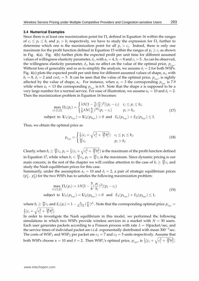
3.4 Numerical Examples

Since there is at least one maximization point for Πi defined in Equation 16 within the rangesof ci ≤ pi ≤ bi and pi > bi respectively, we have to study the expression for Πi further todetermine which one is the maximization point for all pi > ci. Indeed, there is only onemaximum for the profit function defined in Equation 15 within the ranges of pi ≥ ci as shownin Fig. 4(a). Fig. 4(b) further plots the expected profit per unit time for different assumedvalues of willingness elasticity parameter, δi, with αi = 4, bi = 8 and ci = 5. As can be observed,the willingness elasticity parameter, δi, has no affect on the value of the optimal price, piopt

.Without loss of generality and so as to simplify the analysis, we assume δi = 2 for both WSPs.Fig. 4(c) plots the expected profit per unit time for different assumed values of shape, αi, withbi = 8, δi = 2 and costi = 5. It can be seen that the value of the optimal price, piopt

, is sightlyaffected by the value of shape, αi. For instance, when αi = 3 the corresponding piopt

is 7.9while when αi = 13 the corresponding piopt

is 6.9. Note that the shape α is supposed to be avery large number for a normal service. For ease of illustration, we assume αi = 10 and δi = 2.Then the maximization problem in Equation 16 becomes:

maxi∈{1,2}

Πi(pi) =

{

λN[1 − 56 (

pi

bi)2](pi − ci) ci ≤ pi ≤ bi;

16 λN( bi

pi)10(pi − ci) pi > bi,

subject to U1(p1opt) = U2(p2opt

) > 0 and E1(p1opt) + E2(p2opt

) ≤ 1.

(17)

Thus, we obtain the optimal price as

piopt=

{

13 (ci +

√

c2i +

185 b2

i ) ci ≤ pi ≤ bi;109 ci pi > bi.

(18)

Clearly, when bi ≥ 109 ci, pi =

13 (ci +

√

c2i +

185 b2

i ) is the maximum of the profit function defined

in Equation 17, while when bi <109 ci, pi =

109 ci is the maximum. Since dynamic pricing is our

main concern, in the rest of the chapter we will confine attention to the case of bi ≥ 109 ci and

study the Nash equilibrium prices for this case.Summarily, under the assumption αi = 10 and δi = 2, a pair of strategic equilibrium prices(p∗1 , p∗2) for the two WSPs has to satisfies the following maximization problem:

maxi∈{1,2}

Πi(pi) = λN[1 − 5

6(

pi

bi)2](pi − ci)


) > 0 and E1(p1opt) + E2(p2opt

) ≤ 1,

(19)

where bi ≥ 109 ci and Ei(pi) = 1− αi

αi+δi(

pi

bi)δi . Note that the corresponding optimal price piopt

=

13 [ci +

√

c2i +

185 b2

i ].

In order to investigate the Nash equilibrium in this model, we performed the followingsimulations in which two WSPs provide wireless services in a market with N = 30 users.Each user generates packets according to a Poisson process with rate λ = 10packet/sec, andthe service times of individual packet are i.i.d. exponentially distributed with mean 300−1sec.The costs of WSP1 and WSP2 per packet are c1 = 7 and c2 = 5 units respectively. Assume that

both WSPs choose α = 10 and δ = 2. Then WSPi’s optimal price, piopt, is 1

3 [ci +√

c2i +

185 b2

i ].


www.intechopen.com


(a) Expected profit per unit time versus quotedprice (varying scale parameter b)

(b) Expected profit per unit time versus quotedprice (varying willingness elasticity parameter δ)

(c) Expected profit per unit time versus quotedprice (varying willingness elasticity parameter α)

Fig. 4. Expected profit per unit time versus quoted price under different parameters


www.intechopen.com


For the sake of ease of simulation, WSPi’s prices fall into the range of [ci,2ci], which implies

that 109 ci ≤ bi ≤

√

203 ci and 0.167 ≤ Ei(piopt

) ≤ 0.5.

Since a Nash equilibrium would exist when Equation 10 holds, the following expression canbe derived:

p∗1opt− p∗2opt

=5

54λN[(ξ1 +

√

ξ21 +

18

5)

2

− (ξ2 +

√

ξ22 +

18

5)

2

], (20)

where ξ1 = c1b1

and ξ2 = c2b2

. Combining the constraint condition ∑2i=1 Ei(pi) ≤ 1, Nash

equilibrium prices (p∗1opt, p∗2opt

) can be obtained. Evidently, Nash equilibrium prices (p∗1opt, p∗2opt

)

are dependent on the ratio of the cost, ci, and the parameter, bi, of the probabilistic model foruser’s willingness-to-pay.In the simulation, a two-dimensioned numerical search procedure is employed to obtainthe equilibrium prices. The search procedure is described as follows. Firstly, WSPi (i =1,2) determines bi according to algorithm 1 and calculates corresponding piopt

, respectively.Note that here variable bi is used to represent the users’ different responses to the WSPs’quoted prices. For convenience, in the rest of section, piopt

and pi are interchangeable.

Let {p11, p2

1, · · · , pn1} and {p1

2, p22, · · · , pn

2} be optimal price strategy forms of WSP1 and WSP2

respectively. We start by finding the expected user’s compensated utilities with WSP1 andWSP2 respectively, given that WSP0 and WSP1 set their prices according to their optimalprice strategy forms respectively. We first keep WSP1’s price fixed at p1

1, while WSP2’s price

continuously changes according to its price strategy form {p12, p2

2, · · · , pn2}. The continuous

price change allows us to identify the equilibrium compensated utilities, namely U0 = U1.Thus, the equilibrium prices, (p1∗

1 , p1∗2 ), that correspond to the equilibrium compensated

utilities are identified. We then proceed to the next price in {p11, p2

1, · · · , pn1}.

Algorithm 1begin

b11 ← 10

9 c1

for b1 =109 c1 to

√

203 c1 do

bi1 = bi−1

1 + 0.005

b12 ← 10

9 c2

for b2 =109 c2 to

√

203 c2 do

bi2 = bi−1

2 + 0.005end

endend

Fig. 5 illustrates the value difference between U2(p2) and U1(p1), U2(p2)− U1(p1), underdifferent pairs of prices (p1, p2). The pairs of prices that make U2(p2) = U1(p1) are Nashequilibrium prices we are looking for. Note that using the bi obtained according to the abovealgorithm one could only find out pairs of prices (p1, p2) which make U2(p2)− U1(p2) ≈ 0.Here, we actually refer to the pairs of prices (p1, p2) which make U2(p2)−U1(p1)≈ 0 as Nashequilibrium prices, which is represented as (p∗1 , p∗2)Table 1 lists some pairs Nash equilibrium prices and the corresponding acceptance rates. Asis observed, both WSPs have to set their price within a certain range so that the constraint


www.intechopen.com


Fig. 5. U2(p2)− U1(p1)

p1 9.8033 10.77 11.71 12.78 13.28 13.688

E1(p1) 0.3638 0.4118 0.4458 0.4749 0.4861 0.4942

p2 7.114 7.8227 8.6116 9.4802 9.9847 10.236

E2 p2) 0.3727 0.4192 0.4562 0.4859 0.4973 0.5057

Table 1. Nash equilibrium price versus Nash equilibrium acceptance rate

E1(p∗1) + E2(p∗2) ≤ 1 can be satisfied. For instance, as shown in Table 1, when the WSP2 withlower price increases its price higher than twice its cost, E2(p∗2) > 0.5, as a response, WSP1

with higher price also increases its price, which in turn lead to E1(p∗1) + E2(p∗2)> 1. It impliesthat these two WSPs cannot increase their price as high as they want without cooperation.Table 2 lists the user’s compensated utilities with the two WSPs under different prices. Ascan be observed, for example, if WSP1 initially sets its price at 12.906 while WSP2 initiallysets its price as 5.635, U1(p1) < U2(p2) and the users will choose to subscribe or switch toWSP2. Then WSP1 will have to decrease its price to attract more users, while WSP2 wouldincrease its price considering its congestion situation or just leave its price unchanged. Thisprice adjusting process will be repeated until p1 and p2 converge to the point at which thecompensated utility experienced by the users with WSP1, U1, is equal to the compensatedutility experienced by the users with WSP2, U2. For instance, WSP1 decreases its price to11.084 while WSP2 increases its price to 8.112. At this point, U1(p∗1) = U2(p∗2), no WSP hasany incentive to deviate from its price without the cooperation of the other, which may nothappen, until existing users voluntarily disconnect or new users join in.When the number of users in this market N changes, U1(p1) and U2(p2) change accordingly,which in turn leads to the Nash equilibrium moving. This results in another round of priceadjustment among the two WSPs and the users. As shown in Table 3, if we suppose in thefirst round the number of users N = 30 and the two WSPs end up with a Nash equilibriumwith prices p1 = 11.818 and p2 = 8.6976 respectively. When the number of users N increasesor decreases, even if WSP1 keeps its price p1 = 11.818, WSP2 has to change its price suchthat both WSPs and the users can reach a new equilibrium. Additionally, when some userswith one WSP disconnect or some new users join in one WSP, the WSP could adjust its priceconsidering its resource utility or congestion situation. This also could lead to a new round ofadjustment.


www.intechopen.com


p1 8.246 8.995 9.791 10.237 11.084 11.818 12.478 12.906 13.685

U1 222.13 198.83 181.27 173.54 161.64 153.44 147.26 143.73 138.06

p2 5.635 6.602 7.552 7.774 8.112 8.474 9.187 9.452 10

U2 239.16 195.38 171.46 167.29 161.64 156.37 147.75 145.02 140

Table 2. Users’ compensated utilities

Fig. 6. Equilibrium prices for different number of users N

Fig. 6 plots the equilibrium points (at which U1(p∗1)−U2(p∗2)≈ 0) over p1 and p2 for variousN. As can observed, for a given optimal price p1 of WSP1, there is a unique optimal pricep2 of WSP2 so that WSP1 and WSP2 reach Nash equilibrium, and there is a quasi-linearrelationship between p∗1 and p∗2 . It is worth noting that this property is useful for a dynamicpricing competition. Since each optimal price piopt

corresponds to a certain value of bi, whichis determined by the traffic load of WSPi, if we simply assume, for WSPi, bi is varied with thenumber of users arriving at WSPi, sequentially, the optimal price piopt

also varies in responseto the change of the number of the arriving users. Suppose WSP1 and WSP2 set their optimalprices p1 and p2 based on the numbers of their arriving users respectively, but p1 and p2 arenot in equilibrium. The users who receive a lower compensated utility will switch to anotherWSP, which in turn results in an increase of users at one WSP and a decrease of users at thealternative. Accordingly, p1 and p2 vary gradually until they converge to a Nash equilibriumpoint (p∗1 , p∗2).

4. An extended pricing model for wireless oligopolies

In this section, we extend the two-stage noncooperative game model described in Section 3 toa multi-provider setting as shown in Fig. 7.

4.1 Model description

Assume that there is a set I = {0,1,2, . . . , I − 1} of WSPs in a certain area to providewireless services to N potential users. Denote pi and ci as WSPi’s price and cost per packettransmission respectively. Each user generates packets according to a Poisson process withmean rate λ. Then the potentially total mean arrival rate of packets in the whole network isgiven by λN. Note that λN can be seen as an arrival rate when all potential users send out


www.intechopen.com


p1 8.246 8.9975 9.7912 10.237 11.084 11.818 12.112 − −U1 280.15 275.64 272.05 270.39 267.7 265.73 265 − −

N = 5 Π1 14.46 30.64 50.68 62.71 86.63 108.19 117 − −p2 6.1613 6.8438 7.6099 8.0513 8.9159 9.6874 10 − −U2 280.15 275.65 272.05 270.39 267.7 265.72 265 − −Π2 15.90 32.28 53.09 65.78 91.56 115.26 125 − −p1 8.246 8.9945 9.7912 10.237 11.084 11.818 12.478 12.7 −U1 268.55 260.28 253.9 251.02 246.49 243.27 240.77 240 −

N = 10 Π1 28.92 61.28 101.36 125.41 173.27 216.37 256.11 269.61 −p2 6.0265 6.6407 7.3191 7.7071 8.4705 9.1531 9.7964 10 −U2 268.56 260.29 253.89 251.03 246.49 243.27 240.77 240 −Π2 26.09 54.26 89.96 111.7 156.3 197.58 236.68 250 −p1 8.246 8.9945 9.7912 10.237 11.084 11.821 12.481 12.906 13.187

U1 245.34 229.56 217.59 212.28 204.06 198.33 194 191.52 189.99

N = 20 Π1 57.83 122.56 202.71 250.82 346.54 433.11 512.59 584.49 599.03

p2 5.9594 6.5336 7.1592 7.5159 8.2071 8.8205 9.3845 9.7544 10

U2 245.33 229.57 217.59 212.28 204.05 198.34 194.01 191.5 190

Π2 47.74 97.99 162.48 201.78 281.39 354.68 423.58 469.5 500

p1 8.246 8.9945 9.7912 10.237 11.084 11.818∗ 12.478 12.906 13.685

U1 222.13 198.83 181.24 173.54 161.64 153.44 147.26 143.73 138.06

N = 30 Π1 86.75 183.84 304.07 376.23 519.8 649.12 768.32 846.73 991.04

p2 5.9361 6.498 7.105 7.4492 8.1124 8.6976∗ 9.2333 9.5853 10.236

U2 222.13 198.83 181.27 173.54 161.64 153.44 147.26 143.73 138.06

Π2 67.34 141.81 234.96 291.49 405.39 509.75 607.48 672.59 794.28

p1 8.246 8.9975 9.7912 10.237 11.084 11.821 12.478 12.906 13.474

U1 210.53 183.38 163.12 154.17 140.42 130.95 123.89 119.84 115

N = 35 Π1 101.21 214.97 354.74 438.94 606.44 757.95 896.38 987.85 1110.5

p2 5.9303 6.4891 7.09 7.431 8.8049 8.6638 9.1901 9.5358 10

U2 210.48 183.41 161.1 154.14 140.43 130.96 123.88 119.83 115

Π2 77.76 163.91 271.3 336.53 467.33 587.59 699.46 773.97 875

p1 8.246 8.9975 9.7912 10.237 11.084 11.818∗ 12.478 12.909 13.53

U1 198.92 168.11 144.96 134.8 119.21 108.53 100.51 95.91 90

N = 40 Π1 115.67 245.12 405.42 501.64 693.07 865.5 1024.4 1129.7 1282.9

p2 5.9245 6.4801 7.0779 7.4159 8.0635 8.6362∗ 9.1562 9.4988 10

U2 198.93 168.09 144.95 134.78 119.23 108.51 100.51 95.92 90

Π2 87.96 185.66 307.48 381.24 529.1 664.89 791.08 875.37 1000

p1 8.246 8.9945 9.7912 10.237 11.084 11.818∗ 12.481 12.906 13.614

U1 175.72 137.39 108.65 96.06 76.78 63.62 53.72 48.16 39.99

N = 50 Π1 144.58 306.4 506.78 627.06 806.34 1081.9 1281.5 1411.2 1629.6

p2 5.9187 6.4683 7.0599 7.3947 8.0361 8.5962∗ 9.1099 9.4432 10

U2 175.64 137.41 108.69 96.06 76.77 63.63 53.73 48.15 40

Π2 209.95 288.67 517.49 629.44 707.32 842.3 935.83 1087.6 1181.6

Table 3. Users’ compensated utilities for different number of users N


www.intechopen.com


Evalution of

QoS and Benefits

Private Pricing

Strategy Selection

Evalution of Profit

User’s Choice of

a WSP

WSP0

WSP2

Evalution Congestion and

Resource Management

WSP1

WSPI−1

UserUserUser

User

Fig. 7. Pricing model for multiple WSPs

all their requests without considering price or QoS. In addition, we stick to the mathematicaldefinition of user’s utility and compensated utility in Section 3. Then the user’s compensatedutility Ui with WSPi can be expressed as:

Ui = Ui(EDi)− pi = 1/EDi − pi = μ − λNEi(pi)− pi, (21)

where i = 0,1,2, . . . , I − 1.Similar to the duopoly case, from a user’s perspective,

– if Ui < 0 for all i ∈ I, the user will opt out of all the WSPs;

– if Ui > 0 and Ui > U−i, where the subscript −i represents all the WSPs belonging to I

except i itself, the user will subscribe to WSPi;

– only if U0 = · · · = Ui = · · · = UI−1 > 0, the user is indifferent among these WSPs.

In the situation in which the indifference relation

U0(ED0)− p∗0 = · · · = U0(ED0)− p∗i = · · · = UI−1(EDI−1)− p∗I−1 > 0 (22)

holds, all the WSPs and users reach a Nash equilibrium and the set of prices{p∗0 , p∗1 , p∗2 , · · · , p∗I−1} is the Nash equilibrium prices.Similarly, the profit function for WSPi per unit time, Πi, is given by Πi = λNEi(pi)(pi − ci).Thus, solving the following maximization problem gives WSPi’s optimal price at which WSPi

maximizes its profit:

maxΠi(pi) =

{


(pi

bi)δi ](pi − ci) ci ≤ pi ≤ bi;

λN δiαi+δi

( bipi)αi (pi − ci) pi > bi,

(23)

where i = 0,1, . . . , I − 1.According to the previous analysis in Section 3, the maximization problem Equation 23 can bereduced to the following maximization problem:

maxi∈0,1,...,I−1

Πi(pi) = λN[1 − 5

6(

pi

bi)2](pi − ci)ci ≤ pi ≤ bi


) = . . . = UI−1(pI−1opt) > 0

andI−1

∑i=0

Ei(piopt) ≤ 1,

(24)


www.intechopen.com


where bi ≥ 109 ci and Ei(pi) = 1− αi

αi+δi(

pi

bi)δi . Note that the corresponding optimal price piopt

=

13 [ci +

√

c2i +

185 b2

i ].

In the next section, we will show the existence and uniqueness of Nash equilibrium in thisoligopoly model.

4.2 Equilibrium: existence and uniqueness

In equilibrium, the distribution of users among the WSPs has to be stable from a macroperspective, meaning that a new arrival user will randomly subscribe to a particular WSPi

(i = 0,1,2, · · · , I − 1) and the users who already subscribed to a WSP have no incentive toswitch to a different WSP. This indicates that the compensated utilities Ui (i = 0,1,2, · · · , I − 1)should be non-negative and equal to each other for all WSPi (i = 0,1,2, · · · , I − 1). Without lossof generality, we assume that c0 < c1 < c2 < · · · < cI−1. We then take WSP0’s optimal pricep0opt

and cost c0 as references such that the equilibrium price of WSPi (i = 1,2, · · · , I − 1) canbe expressed as a function of p0opt

and c0. The condition that all the compensated utilities Ui

(i = 0,1,2, · · · , I − 1) are equal in equilibrium can be expressed as:

μ − λNE(p0opt)− p0opt

= μ − λNE(piopt)− piopt

, (25-1)

where Ei(pi) = 1 − 5

6(

pi

bi)2; (25-2)

and piopt=

1

3(ci +

√

c2i +

18

5b2

i ), (25-3)

(25)

for all i = 0,1,2, · · · , I − 1.From Equation 25-3, we obtain:

6b2i = 15p2

iopt− 10piopt

ci. (26)

Substituting bi into Equation 25-2, we get:

Ei(piopt) = 1 −

piopt

3piopt− 2ci

. (27)

Substituting Ei(piopt) into Equation 25-1 results in:

piopt− p0opt

= λN(piopt

3piopt− 2ci

−p0opt

3p0opt− 2c0

). (28)

Dividing p0opton both sides of Equation 28 and denoting

piopt

p0optby ξi, we have

ξi − 1 = λN(ξi

3piopt− 2ci

− 1

3p0opt− 2c0

). (29)

Substituting6b2

i5piopt

for 3piopt− 2ci, Equation 29 can be rewritten as:

ξi(5piopt

λN

6b2i

− 1) =5p0opt

λN

6b20

− 1. (30)


www.intechopen.com


Dividing p0opton both sides of Equation 30 again, we can obtian

ξi(5ξiλN

6b2i

− 1

p0opt

) =5λN

6b20

− 1

p0opt

. (31)

Here Equation 31 is a quadratic equation in ξi, which can be rewritten as:

a1ξ2i + a2ξi + a3 = 0. (32)

where

a1 =5λN

6b2i

, a2 = − 1

p0opt

, a3 =1

p0opt

− 5λN

6b20

.

The solutions to Equation 32 are−a2±

√a2

2−4a1a3

2a1, in which

a22 − 4a1a3 =

1

p20opt

+25λ2N2

9b20b2

i

− 10λN

3p0optb2

i

.

It is straightforward to prove that 25λ2 N2

9b20b2

i

>10λN

3p0optb2

i

given that 5p0optλN > 6b2

0, which can be

rewritten as λN > 3p0opt− 2c0. Later we will show that p0opt

≤ 2c0. Thus λN > 3p0opt− 2c0 ≥

4c0. Note that λN represents the mean rate that all N users generate packets per secondwhile c0 is WSP0’s per packet transmission. Therefore c0 cannot be directly compared to λN.However, it is reasonable to assume that the cost per packet can be converted into a smallenough unit such that c0 << λN, which means 5p0opt

λN >> 6b20 always holds.

Since 25λ2 N2

9b20b2

i

>10λN

3p0optb2

i

, it can be proved that a22 − 4a1a3 >

1p2

0opt

> 0 and√

a22 − 4a1a3 > −a2,

meaning that the solutions to Equation 32 are real numbers and only one of them is positive.Note that piopt

for all i = 0,1,2, · · · , I − 1 are positive. Therefore Equation 32 has a unique

solution, which is a positive real number (−a2+

√a2

2−4a1a3

2a1). Now it can be concluded that for

all i = 1,2, · · · , I − 1, pioptis linear with p0opt

with a coefficient ξi =−a2+

√a2

2−4a1a3

2a1. In other

words, under the constraint ∑I−1i=0 Ei(piopt

) ≤ 1, for an arbitrary p0opt, there exists a unique piopt

(i = 1,2, · · · , I − 1) in equilibrium with it.Furthermore, by investigating the unique solution to Equation 32, we find that ξi ≈

1p0opt

+√

25λ2 N2

9b20 b2

i5λN

3b2i

>bib0

. Let bib0

be ki. Thus ξi = γiki, where γi∼=

1p0opt5λN

3b2i

+ 1. It can be proved that γi

approximates to 1 but is strictly greater than 1. According to Equation 26,

k2i =

b2i

b20

=3p2

iopt− 2piopt

ci

3p20opt

− 2p0optci

=3γ2

i k2i p2

0opt− 2γiki p0opt

ci

3p20opt

− 2p0optci

. (33)

Solving Equation 33, ki is given by

ki =2γici

3γ2i p0opt

− 3p0opt+ 2c0

. (34)

Since γi∼= 1, ki

∼= γicic0

.


www.intechopen.com


In summary,piopt

p0opt

∼= γibib0

∼= γ2i

cic0

, where γi∼= 1, and under the constraint ∑

I−1i=0 Ei(piopt

)≤ 1, for

an arbitrary p0opt, the higher the cost ci the greater γi, meaning for WSPi the higher the cost ci

the higher the corresponding equilibrium price, piopt.

The constraint ∑I−1i=0 Ei(piopt

) ≤ 1 can be expressed as:

I − 5

6(

p20opt

b20

+p2

1opt

b21

+ · · ·+p2

I−1opt

b2I−1

)

=I − 5

6

p20opt

b20

(1 + γ21 + · · ·+ · · ·+ γ2

I−1)

≈I − I5

6

p20opt

b20

=IE0(p0opt) ≤ 1.

(35)

Here Equation 35 indicates that the maximum value of E0(p0opt), which is denoted by E0max

,

approximates to 1I . The corresponding optimal price is denoted as the maximum optimal

price p0max. Then, it is straightforward to prove that the greater the number of providers I the

lower the maximum optimal price p0maxthat WSP0 could reach. This in turn means that, in

equilibrium, all other WSPs’ maximum optimal prices, pimaxfor all i = 1,2, · · · , I − 1, are lower

accordingly. Thus, when more WSPs enter into the market, in equilibrium, the maximumprices they can charge decreases.

4.3 Numerical examples

In order to verify the analytical results obtained in the previous section, we performed thefollowing simulations where several WSPs provide wireless services in a market with N = 40users. Each user generates packets according to a Poisson process with rate λ = 10packet/sec,and the service time of individual packet are i.i.d. exponentially distributed with mean300−1sec.To study the impact of an entry of a new WSP on the existing WSPs, we first conducted asimulation where there are two WSPs: WSP0 and WSP1 competing in the market. The costsof WSP0 and WSP1 per packet are c0 = 5 and c1 = 7 units respectively. For convenience, inthe rest of section, piopt

and pi are interchangeable. Let {p10, p2

0, · · · , pn0} and {p1

1, p21, · · · , pn

1}be optimal price strategy forms of WSP0 and WSP1 respectively. Using the same approachthat we used to identify the equilibrium in Section 3, we find the set of the equilibrium prices{(p1∗

0 , p1∗1 ), (p2∗

0 , p2∗1 ), . . . , (pn∗

0 , pn∗1 )}, which is represented as (p∗0 , p∗1) in the rest of the section.

Fig. 8(a) plots (p∗0 , p∗1). As can be seen, in equilibrium, for an arbitrary p∗0 , there is a uniquep∗1 corresponding to it. In particular, p∗0 is quasi-linear with p∗1 . Under the same assumptions,p∗0max

and p∗1maxare 9.997 and 13.526 respectively.

We then simulated another scenario where the third WSP, WSP2, joins WSP0 and WSP1.WSP2’s cost per packet c2 = 9 units and its optimal price strategy form is {p1

2, p22, · · · , pn

2}.

Using the same approach, we obtained the equilibrium prices (p′∗0 , p

′∗1 , p

′∗2 ), which are plotted

in Fig. 8(b) to compare with those obtained from the two-WSP scenario. As can be observed, in

equilibrium, for an arbitrary p′∗0 , there are unique p

′∗1 and p

′∗2 corresponding to it respectively.

Again, p′∗0 is linear with p

′∗1 and p

′∗2 respectively. In addition, the range of values for the

equilibrium prices (p∗0 , p∗1) in two-WSP case shown in Fig. 8(a) is larger than that in three-WSP


www.intechopen.com


Fig. 8. Equilibrium prices: two-WSP scenario vs three-WSP scenario

case shown in Fig. 8(b). This is because of the equilibrium condition ∑I−1i=0 Ei(piopt

) ≤ 1∀i = 0,1,2, · · · , I − 1, which restricts the allowed values for p∗i as analyzed in Equation 35.When the number of WSPs increases to 3 from 2, under the same assumptions, the maximum

equilibrium prices p′∗0max

and p′∗1max

are 6.623 and 9.186 respectively. Evidently, p′∗0max

and p′∗1max

are significantly lower than those obtained in two-WSP scenario.Fig. 9 illustrates the expected profits of all WSPs associated with the equilibrium prices plottedin Fig. 8. Similarly, the range of the values for the expected profit in two-WSP case is largerthan that of three-WSP case. As we can see, in three-WSP scenario, the expected profits ofWSP0 and WSP1 are lower than those of two-WSP scenario, because WSP2 takes some marketshare.When the number of potential users, N, in this market changes, the expected compensatedutility Ui changes, which in turn changes the current Nash equilibrium. This leads to anotherround of price adjustment among the WSPs and the users. Table 3 lists some equilibriumprices, the corresponding expected compensated utilities and the corresponding expectedacceptance rate with various number of potential users, N. As shown in Table 3, if we supposein the first round N = 30 and the three WSPs end up with a Nash equilibrium with p0 = 6.2970,p1 = 8.7274 and p2 = 11.114. When the number N changes, even if WSP0 keeps its pricep0 = 6.2970 unchanged, WSP1 and WSP2 have to change their price such that the three WSPsand the users can reach a new equilibrium.It has been shown that, with the proposed pricing scheme, when a new WSP enters into amarket with two or more WSPs already existing, the maximum equilibrium prices that theexisting WSPs can reach will decrease. For a WSP, besides its traffic load status, cost is anotherfactor determining its optimal prices, which in turn affects the WSPs’ equilibrium prices.Thus, a follow-up question would be how the cost of the new WSP affects the equilibriumprices of the existing WSPs. Then another three-WSP scenario simulation, in which costs


www.intechopen.com


p0 5.7624 5.7769 5.9918 6.1528 6.2970∗ 6.3827 6.4864 6.5726 6.9011

U0 273.31 273.03 269.09 266.59 264.53 263.39 262.09 261.06 257.58

E0 0.2092 0.2120 0.2487 0.2726 0.2918 0.3023 0.3143 0.3236 0.3552

p1 7.9153 7.9325 8.2041 8.4020 8.5776∗ 8.6833 8.807 8.9133 9.3052

N = 10 U1 273.30 273.03 269.10 266.58 266.53 263.38 262.10 261.05 257.56

E1 0.1878 0.1904 0.2262 0.2502 0.2689 0.2794 0.2912 0.3004 0.3313

p2 10.003 10.023 10.336 10.565 10.766∗ 10.885 11.026 11.146 11.583

U2 273.29 273.03 269.09 266.58 264.54 263.39 262.10 261.06 259.57

E2 0.1670 0.1695 0.2051 0.2285 0.2470 0.2573 0.2690 0.2780 0.3084

p0 5.6587 5.7769 5.9918 6.1528 6.2970∗ 6.3827 6.4864 6.5726 6.7395

U0 256.57 251.83 244.26 239.33 235.35 233.16 230.66 228.70 225.17

E0 0.1888 0.2120 0.2487 0.2607 0.2918 0.3023 0.3143 0.3240 0.3405

p1 7.8493 8.0045 8.2883 8.4984 8.6862∗ 8.7982 8.9340 9.0436 9.2575

N = 20 U1 256.57 251.87 244.28 239.36 235.38 233.17 230.64 228.70 225.18

E1 0.1779 0.2010 0.2372 0.2726 0.2797 0.2902 0.3021 0.3113 0.3278

p2 10.003 10.195 10.539 10.792 11.017∗ 11.152 11.314 11.444 11.699

U2 256.59 251.83 244.26 239.38 235.15 233.15 230.63 228.70 225.16

E2 0.1670 0.1899 0.2260 0.2493 0.2680 0.2785 0.2903 0.2993 0.3157

p0 5.6243 5.7769 5.9918 6.1528 6.2970∗ 6.3827 6.4864 6.5726 6.6828

U0 239.88 230.64 219.39 212.07 206.17 202.93 199.23 196.33 192.84

E1 0.1817 0.2120 0.2487 0.2726 0.2918 0.3023 0.3143 0.3236 0.3349

p1 7.8264 8.0305 8.3203 8.5365 8.7274∗ 8.8424 8.9784 9.0940 9.2397

N = 30 U1 239.87 230.70 219.40 212.05 206.19 202.91 199.25 196.31 192.81

E1 0.1744 0.2042 0.2409 0.2647 0.2836 0.2941 0.3059 0.3153 0.3265

p2 10.003 10.258 10.614 10.879 11.114∗ 11.255 11.420 11.562 11.737

U2 239.89 230.65 219.42 212.09 206.21 202.92 199.27 196.31 192.84

E2 0.1670 0.1970 0.2332 0.2568 0.2756 0.2861 0.2977 0.3071 0.3181

p0 5.6071 5.7769 5.9918 6.1528 6.2970∗ 6.3827 6.4864 6.5726 6.6559

U0 223.20 209.44 194.52 184.81 177 172.70 167.80 163.97 160.44

E0 0.1780 0.2120 0.2487 0.2726 0.2918 0.3023 0.3143 0.3233 0.3323

p1 7.8149 8.0449 8.3378 8.5541 8.7481∗ 8.8660 9.0021 9.1208 9.2307

N = 40 U1 223.18 209.48 194.49 184.84 177.04 172.64 167.85 164.01 160.43

E1 0.1726 0.2062 0.2429 0.2665 0.2855 0.2962 0.3079 0.3172 0.3258

p2 10.003 10.29 10.655 10.926 11.167∗ 11.311 11.479 11.622 11.761

U2 223.19 209.53 194.54 184.81 177 172.65 167.85 164.02 160.44

E2 0.1670 0.2005 0.2370 0.2607 0.2796 0.2901 0.3017 0.3109 0.3195

p0 5.5956 5.7769 5.9918 6.1528 6.2970∗ 6.3827 6.4864 6.5726 6.6381

U0 206.65 188.25 169.65 157.56 147.82 142.47 136.37 131.60 128.14

E0 0.1775 0.2141 0.2510 0.2750 0.2944 0.3048 0.3166 0.3262 0.3304

p1 7.8064 8.0507 8.3466 8.56 8.7657∗ 8.8779 9.0199 9.1356 9.2218

N = 50 U1 206.58 188.46 169.68 157.57 147.79 142.48 136.31 131.59 128.19

E1 0.1712 0.2082 0.2453 0.2689 0.2880 0.2986 0.3103 0.3197 0.3252

p2 10 10.31 10.681 10.955 11.199∗ 11.343 11.518 11.663 11.773

U2 206.67 188.37 169.62 157.51 147.81 142.47 136.38 131.57 128.12

E2 0.1667 0.2026 0.2394 0.2633 0.2820 0.2924 0.3042 0.3135 0.3202

Table 4. Equilibrium prices, expected compensated utilities and expected acceptance rates fordifferent number of users N


www.intechopen.com


p′∗0max

p′∗1max

c2 = 1 6.5428 9.0792c2 = 3 6.6559 9.2307

c0 = 5 c2 = 9 6.6232 9.1861c1 = 7 c2 = 13 6.5964 9.1534

c2 = 20 6.5815 9.1297

Table 5. Maximum equilibrium prices of WSP0 and WSP1 (p′∗0 , p

′∗1 ) for three-WSP scenario

with various cost of WSP2.

of WSP0 and WSP1 are kept unchanged while WSP2’s cost varies, was conducted. Fig.

10 presents the equilibrium prices (p′∗0 , p

′∗1 ) with WSP2 taking different costs. For ease of

illustration, the maximum equilibrium prices corresponding to Fig. 10 (a), (b) and (c) are listedin Table 5. It can be observed that when WSP2’s cost is lower than costs of WSP0 and WSP1,in equilibrium, the maximum prices that WSP0 and WSP1 could reach are lower compared tothe case where WSP2’cost is higher than the costs of WSP0 and WSP1. For the latter case, theentry of a new WSP with a higher cost results in slight lower maximum equilibrium prices forboth WSP0 and WSP1.

5. Advanced thoughts

The presented material can be usefully extended in a number of ways. In this section only theextensions will be identified and potential game theory modeling modes indicated.Firstly an assumption in the section on the basic wireless duopoly was that all users show thesame basic behavior. Relaxing this, a competition between the WSPs and a set of N types ofusers can be described. The N types of users could describe economic, social or regulatorygroupings that have differing QoS and price utility definitions. This would allow for thedevelopment of a scaled preference analysis that could be used to gauge more accurately

Fig. 9. Expected profits associated with equilibrium prices in Fig. 8


www.intechopen.com


Fig. 10. Equilibrium prices of WSP0 and WSP1 (p′∗0 , p

′∗1 ) for three-WSP scenario with various

cost of WSP2.

the social benefits of regulated access to the wireless bandwidth. Secondly the analysis ofoligopoly based pricing depends on the assumption of a mature market where entrances andexits by WSPs are not relevant. In actual fact this is quite unrealistic and can profitably beexpanded to take into account changes in the number of WSPs during a period and the impacton both relative profit and market share. Finally by changing the analysis basis queue toa more dynamic queue with memory effect models of user churn and brand loyalty can bedeveloped that could show the benefit of branding compaigns.

6. References

Altman, E., Barman, D. & Azouzi, R. E. (2006). Pricing Differentiated Services: AGame-Theoretic Approach, Computer Networks 50: 982–1002.

Altman, E. & Basar, T. (1998). Multiuser Rate-Based Flow Control, IEEE Transactions onCommunication 46: 940–949.

Altman, E. & Wynter, L. (2002). Equilibrium, Games and Pricing in Transportation andTelecommunication Networks, Technical Report 4632, IRISA .

Armony, M. & Haviv, M. (2003). Price and Delay competition Between Two Service Providers,European Journal of Operational Research 147: 32–50.

Basar, T. & Srikant, R. (2002). Revenue-maximizing Pricing and Capacity Expansion in aMany-user Regime, Proceedings of the 21st Annual Joint Conference of the IEEE Computerand Communications Societies (IEEE INFOCOM 2002), New York, USA.


www.intechopen.com


Cao, X., Shen, H., Milito, R. & Wirth, P. (2002). Internet Pricing with a Game TheoreticalApproach: Concepts and Examples, IEEE/ACM Transactions on Networking10: 208–216.

Das, S. K., Chatterjee, M. & Lin, H. (2004). An Econometric Model for Resource Managementin Competitive Wireless Data Networks, IEEE Network Magazine 18(6): 20–26.

Dziong, Z. & Mason, L. (1996). Fair-efficient Call Admission Control Policies for BroadbandNetwork - A Game Theoretical Approach, IEEE/ACM Transactions on Networking4: 123–136.

Gibbens, R., Mason, R. & Steinberg, R. (2000). Internet Service Classes under Competition,IEEE Journal on Selected Areas in Communications 18(7): 2490–2498.

Hock, N. C. (1996). Queuing Modeling Fundamentals, John Wiley and Sons Ltd.Jagannatha, S., Nayak, J., Almeroth, K. & Hofmann, M. (2002). A Model for Discovering

Customer Value for E-content, Proceedings of the Eighth ACM SIGKDD InternationalConference on Knowledge Discovery and Data Mining, Edmonton, Alberta, Canada,pp. 23–26.

Kao, Y. & Huan, J. (2008). Price-based Resource Allocation for Wireless Ad Hoc Networkswith Multi-rate Capability and Energy Constraints , Computer Communications31: 3613–3624.

Kelly, F. P. (2000). Models for A Self-Managed Internet, Philosophical Transactions of the RoyalSociety A358: 2335–2348.

Kelly, F. P., Mauloo, A. K. & Tan, D. K. H. (1998). Rate Control in Communication Networks:Shadow Prices, Proportional Fairness and Stability, Journal of the Operational ResearchSociety 49: 237–252.

Khan, S. Q. (2005). Optimizing Providers’ Profit in Per Networks Applying Automatic Pricingand Game Theory, PhD thesis, The University of Kansas .

La, R. J. & Anantharam, V. (1999). Network Pricing using Game Theoretic Approach,Proceedings of 38th IEEE Conference on Decision and Control, Vol. 4, Phoenix, AZPiscataway, NJ, pp. 4008–4013.

La, R. J. & Anantharam, V. (2002). Utility-based Rate Control in the Internet for Elastic Traffic,IEEE/ACM Transactions on Networking 10(2): 272–286.

Lam, R. K., Chiu, D. & Lui, J. C. S. (2007). On the Access Pricing and Network Scaling Issuesof Wireless Mesh Networks, IEEE transactions on Computers 56: 1456–1469.

Lam, R. K., Lui, J. C. S. & Chiu, D. (2006). On the Access Pricing Issues of WirelessMesh Networks, Proceedings of the 26th IEEE International Conference on DistributedComputing Systems (ICDCS 2006), Lisboa, Portugal.

Low, S. H. & Lapsley, D. E. (1999). Optimization Flow Control: Basic Algorithm andConvergence, IEEE/ACM Transactions on Networking 7(6): 861–874.

Luthi, M., Nadjm-Tehrani, S. & Curescu, C. (2006). Comparative Study of Price-basedResource Allocation Algorithms for Ad Hoc Networks, Proceedings of the 20thInternational Parallel and Distributed Processing Symposium (IPDPS 2006), RhodesIsland, Greece.

M. Bouhtou, M. D. & Wynter, L. (2003). Capacitated Network Revenue Management throughShadow Pricing, Networked Group Communication 2816: 342–351.

Mandjes, M. (2003). Pricing Strategies under Heterogeneous Service Requirements, ComputerNetworks 42(2): 231–249.

Musacchio, J. & Walrand, J. (2006). WiFi Access Point Pricing as a Dynamic Game, IEEE/ACMTransactions on Networking 14: 289–301.


www.intechopen.com


Parsons, S., Gmytrasiewicz, P. J. & Wooldridge, M. J. (2002). Game Theory and Decision Theoryin Agent-Based Systems, Kluwer Academic Publishers.

Qiu, Y. & Marbach, P. (2003). Bandwith Allocation in Ad-Hoc Networks: A Price-BasedApproach, Proceedings of the 22nd Annual Joint Conference of the IEEE Computer andCommunications Societies (IEEE INFOCOM 2003), Vol. 2, San Francisco, California,USA, pp. 797–807.

Ros, D. & Tuffin, B. (2004). A Mathematical Model of the Paris Metro Pricing Scheme forCharging Packet Network, Computer Networks 46: 73–85.

Sakurai, H., Kasahara, S. & Adachi, N. (2003). Internet Pricing and User Opt-out Strategyunder two ISPs Competition, IEICE Technical Report (Institute of Electronics, Informationand Communication Engineers) 102(694(IN2002 233-305)): 153–156.

Shu, J. & Varaiya, P. (2003). Pricing Network Services, Proceedings of the 22nd Annual JointConference of the IEEE Computer and Communications Societies (IEEE INFOCOM 2003),San Franciso, CA, USA.

Tassiulas, L., Kar, K. & Sarkar, S. (2001). A Simple Rate Control Algorithm for MaximizingTotal User Utility, Proceedings of the 20th Annual Joint Conference of the IEEE Computerand Communications Societies (IEEE INFOCOM 2001), Vol. 1, Anchorage, Alaska, USA,pp. 133–141.

Wang, X. & Schulzrinne, H. (1999). RNAP: A Resource Negotiation and Pricing Protocol,Proceedings of International Workshop on Network and Operating System Support forDigital Audio and Video (NOSSDAV’99), Basking Ridge, New Jersey, pp. 77–93.

Xue, Y., Li, B. & Nahrstedt, K. (2003). Price-based Resource Allocation in Wireless Ad HocNetworks, Proceedings of the 11th International Conference on Quality of Service (IWQoS2003), Berkeley, CA, USA.

Xue, Y., Li, B. & Nahrstedt, K. (2006). Optimal Resource Allocation in Wireless Ad HocNetworks: A Price-Based Approach, IEEE transactions on mobile computing 5: 347–364.

Yaıche, H., Mazumdar, R. R. & Rosenberg, C. (2000). A Game Theoretic Framework forBandwidth Allocation and Pricing in Broadband Networks, IEEE/ACM Transactionson Networking 8: 667–678.

Zemlianov, A. & de Veciana, G. (2005). Cooperation and Decision-Making in a WirelessMulti-Provider Setting, Proceedings of 24th Annual Joint Conference of the IEEE Computerand Communications Societies (IEEE INFOCOM 2005), Miami, FL, USA.

Zhang, Z., Dey, D. & Tan, Y. (2008). Price and QoS Competition in Data CommunicationServices, European Journal of Operational Research 187: 871–886.

Zhu, H., Nel, A. & Clarke, W. (2009). A Duopoly Pricing Model for Wireless Mesh Networksunder Congestion-sensitive Users, South African Institute of Electrical Engineers AfricaResearch Journal 100: 48–58.


www.intechopen.com

Wireless Mesh NetworksEdited by Nobuo Funabiki

ISBN 978-953-307-519-8Hard cover, 308 pagesPublisher InTechPublished online 14, January, 2011Published in print edition January, 2011

InTech EuropeUniversity Campus STeP Ri Slavka Krautzeka 83/A 51000 Rijeka, Croatia Phone: +385 (51) 770 447 Fax: +385 (51) 686 166www.intechopen.com

InTech ChinaUnit 405, Office Block, Hotel Equatorial Shanghai No.65, Yan An Road (West), Shanghai, 200040, China

Phone: +86-21-62489820 Fax: +86-21-62489821

The rapid advancements of low-cost small-size devices for wireless communications with their internationalstandards and broadband backbone networks using optical fibers accelerate the deployment of wirelessnetworks around the world.â€¨The wireless mesh network has emerged as the generalization of theconventional wireless network. However, wireless mesh network has several problems to be solved beforebeing deployed as the fundamental network infrastructure for daily use. The book is edited to specify someproblems that come from the disadvantages in wireless mesh network and give their solutions with challenges.The contents of this book consist of two parts: Part I covers the fundamental technical issues in wireless meshnetwork, and Part II the administrative technical issues in wireless mesh network,. This book can be useful asa reference for researchers, engineers, students and educators who have some backgrounds in computernetworks, and who have interest in wireless mesh network. It is a collective work of excellent contributions byexperts in wireless mesh network.

How to referenceIn order to correctly reference this scholarly work, feel free to copy and paste the following:

Andre Nel and Hailing Zhu (2011). Wireless Service Pricing under Multiple Competitive Providers andCongestion-Sensitive Users, Wireless Mesh Networks, Nobuo Funabiki (Ed.), ISBN: 978-953-307-519-8,InTech, Available from: http://www.intechopen.com/books/wireless-mesh-networks/wireless-service-pricing-under-multiple-competitive-providers-and-congestion-sensitive-users

© 2011 The Author(s). Licensee IntechOpen. This chapter is distributedunder the terms of the Creative Commons Attribution-NonCommercial-ShareAlike-3.0 License, which permits use, distribution and reproduction fornon-commercial purposes, provided the original is properly cited andderivative works building on this content are distributed under the samelicense.

https://creativecommons.org/licenses/by-nc-sa/3.0/

wireless service pricing under multiple competitive providers and

Documents