WORKING PAPER

Nr. 179 · May 2017 · Hans-Böckler-Stiftung

LONG-TERM EFFECTS OF FISCAL STIMULUS

AND AUSTERITY IN EUROPE

May, 2017

Sebastian Gechert, Gustav Horn, Christoph Paetz1

ABSTRACT

We analyze whether there are negative (positive) long-term effects of austerity measures

(stimulus measures) on potential output growth. Based on the approach of Blanchard and

Leigh (2013) and Fatás and Summers (2016) and using a novel dataset of narratively iden-

tified fiscal policy shocks, we estimate the impact of these shocks on potential output. We

robustly find strong and persistent long-run multiplier effects for most European Countries in

the early years after the financial crisis and subsequent Euro Area crisis. We conclude that

early stimulus was beneficial even in the long-run, while the subsequent turn to austerity

was badly timed and thus not only deepened the crisis but caused evitable hysteresis ef-

fects.

Keywords: Fiscal Consolidation; Fiscal Multipliers; Forecast Errors; Hysteresis

JEL classification: E62, H68

1 Macroeconomic Policy Institute (IMK). Corresponding author: Sebastian-Gechert@boeckler.de. We would like to thank Achim Truger, Antonio Fatas, Karel Havik, Katja Heinisch, Oana Furtuna, Rudolf Zwiener and Wouter van der Wielen for helpful discussions and data access. All remaining errors are our own.

—————————

Long-term effects of fiscal stimulus and austerity in Europe

Sebastian Gechert, Gustav Horn, Christoph Paetz1

May, 2017

We analyze whether there are negative (positive) long-term effects of

austerity measures (stimulus measures) on potential output growth. Based on

the approach of Blanchard and Leigh (2013) and Fatás and Summers (2016)

and using a novel dataset of narratively identified fiscal policy shocks, we

estimate the impact of these shocks on potential output. We robustly find

strong and persistent long-run multiplier effects for most European Countries

in the early years after the financial crisis and subsequent Euro Area crisis.

We conclude that early stimulus was beneficial even in the long-run, while

the subsequent turn to austerity was badly timed and thus not only deepened

the crisis but caused evitable hysteresis effects.

Keywords: Fiscal Consolidation; Fiscal Multipliers; Forecast Errors; Hysteresis

JEL classification: E62, H68

1. Introduction

Output in many European countries is still below pre-crisis potential. The recession takes

considerably longer compared to past downturns and recovery is long overdue. Forecasts by the

European Commission (EC) or the International Monetary Fund (IMF) in the aftermath of the crisis

assumed a quick recovery to previous trends, but had to be revised downwards several times. These

revisions most strikingly concerned not only GDP but also potential GDP forecasts. Figures 1 and 2

show repeated over-optimism of GDP and potential output forecasts for the EU as a whole and Greece

as an extreme example.2

1 Macroeconomic Policy Institute (IMK). Corresponding author: Sebastian-Gechert@boeckler.de. We would like to thank Achim Truger, Antonio Fatas, Karel Havik, Katja Heinisch, Oana Furtuna, Rudolf Zwiener and Wouter van der Wielen for helpful discussions and data access. All remaining errors are our own.

2 Apart from Germany in all other major European countries potential output growth rates decreased considerably and are now below pre-crisis figures. Potential output estimates were revised downwards both for forecasted and past values in most European countries, apart from Spain.

1

[Figure 1 about here]

[Figure 2 about here]

The persistent and systematic forecast errors call into question the structure and assumptions of the

forecasting models employed. Clearly, the financial crisis and the subsequent crisis of the Euro Area

were extreme events, whose dynamics and channels of impact might be quite different from more

tranquil times. A number of influential factors that unexpectedly drove the severity of the crisis have

been discussed, among them the fragility of the financial system, private sector deleveraging,

increased uncertainty of private agents, current account imbalances, monetary policy constraints,

sustainability of public finances or the impact of discretionary fiscal policy.

In the present paper, we focus on fiscal policy, while we take into account the others. We ask

whether the post-2009-shift towards fiscal consolidation had an unexpectedly substantial negative and

persistent impact on GDP and potential output, in particular in the EU and the Euro Area, which could

be a major explanatory factor for the second recessionary dip that followed in due course and the

persistent gap to pre-crisis GDP trend and unemployment levels. This is equivalent to asking whether

there was an underestimation of fiscal multipliers and, more importantly, their persistence.

Since the crisis, there has been an intense debate and a growing literature on short-run fiscal

multiplier effects (Gechert 2015, Hebous 2011, Mineshima et al. 2014). Expansionary confidence

effects of austerity have been discussed widely3 (Alesina and Ardagna 2010) but have been found to

be rather special cases (Perotti 2011). The general consensus among international institutions now

seems to read that austerity reduces growth in the short run, can be particularly harmful during

downturns and may even increase public debt-to-GDP ratios in the interim (Cottarelli and Jaramillo

2012, Furman 2016).

3 Indeed, official statements by leading policy makers at the time seemed to assume a strong confidence effect of fiscal consolidation that would imply expansionary effects, i.e. negative multipliers. “My understanding is that an overwhelming majority of industrial countries are now in those uncharted waters, where confidence is potentially at stake. Consolidation is a must in such circumstances.” (Trichet 2010) “All the eurozone governments need to demonstrate convincingly their own commitment to fiscal consolidation so as to restore the confidence of markets, not to speak of their own citizens.” (Schäuble 2010)

2

The long-term effects - although they are much more important in terms of welfare and

sustainability of public finances - have attracted far less attention in the empirical literature and remain

more controversial, except for the special case of public investment (Bom and Ligthart 2014).

Certainly, robust inference is much harder to achieve for longer horizons, which might explain the lack

of evidence. For the few exceptions, the dominant reading seems to be that while austerity brings

short-run pain, it provides long-term gain in terms of reduced tax distortions and debt risk (Born et al.

2015, Rogoff 2012). DeLong and Summers (2012) on the other hand make the case for hysteresis

effects where austerity in a deep slump would be self-defeating even in the long run.

The present paper builds on Blanchard and Leigh (2013) (BL hereafter) and Fatás and Summers

(2016) (FS hereafter). BL exploit GDP growth forecast errors for European countries during the 2010-

11 period to create a counterfactual of expected policy impact. They then regress these forecast errors

on planned consolidation for the same sample in order to test whether the impact of consolidation was

underestimated. They find a strong negative correlation between consolidation attempts and output

revisions meaning that countries with bigger consolidation plans faced more severe growth

disappointments – i.e. multipliers had been underestimated by forecasters. FS confirm the findings of

BL with more recent data and extend their method by a second stage, where they regress longer-term

potential output forecast errors on the GDP forecast errors that were arguably caused by the

underestimation of multiplier effects. The coefficient of this second stage can be interpreted as a

measure of persistence of these multiplier effects.

This paper provides two central innovations: (i) We argue that the measure of exogenous fiscal

shocks employed by BL and FS, the change in the structural balance, may face endogeneity issues, as

its calculation is based on potential output itself. We therefore opt for a narrative measure of the fiscal

stance, the Discretionary Fiscal Effort (DFE), as provided by the AMECO database (EC 2013). (ii) We

rigorously test the robustness of our findings and those of FS in terms of omitted variable biases,

outliers, alternative estimation techniques, data sources and sample periods.

We find a significant underestimation of fiscal multipliers of about 0.8 units on average, which is

strong, but still somewhat less pronounced than in BL and FS. These effects have a permanent impact

as measured by five-year-ahead forecasts, making a strong case for hysteresis effects of fiscal

3

consolidation. Our findings are robust to a large set of perturbations. Yet, as a plausible qualification,

we find a weakening of the effects in later crisis years, in line with the slowdown of consolidation,

learning effects or regime-dependent multiplier effects (Auerbach and Gorodnichenko 2012, Baum et

al. 2012). Moreover, some Eastern European countries are influential outliers that weaken the relation

to some extent. The effects seem to be stronger for spending than for revenue shocks. We conclude

that for most countries and during a deep downturn, consolidation is harmful even in the longer-term

and ineffective in achieving longer-term debt sustainability.

The remainder of the paper is organized as follows. Section 2 explains our approach and dataset.

Section 3 presents the baseline results. Section 4 checks the robustness of these findings. The final

section concludes.

2. Method and Data

First Stage: Underestimation of Fiscal Multipliers

In line with BL, we regress the forecast error (fe) of cumulated GDP growth for the years of 2010

(=t) and 2011 for country i on planned (f) fiscal consolidation for the very same period:

∆𝑌𝑌𝑖𝑖,𝑡𝑡:𝑡𝑡+1𝑓𝑓𝑓𝑓 = 𝛼𝛼 + 𝛽𝛽Δ𝐹𝐹𝑖𝑖,𝑡𝑡:𝑡𝑡+1|𝑡𝑡

𝑓𝑓 (+𝑋𝑋𝑖𝑖𝜃𝜃) + ε𝑖𝑖,𝑡𝑡:𝑡𝑡+1|𝑡𝑡 (1)

where

∆𝑌𝑌𝑖𝑖,𝑡𝑡:𝑡𝑡+1𝑓𝑓𝑓𝑓 ≡ ∆𝑌𝑌𝑖𝑖,𝑡𝑡:𝑡𝑡+1 − ∆𝑌𝑌𝑖𝑖,𝑡𝑡:𝑡𝑡+1|𝑡𝑡

𝑓𝑓 (2)

is the forecast error of GDP as given by the difference between current-vintage figures of the

cumulated growth rate of GDP over 2010 and 2011 and its forecast in the vintage of spring 2010. This

figure is negative for most countries during this period. Δ𝐹𝐹𝑖𝑖,𝑡𝑡:𝑡𝑡+1|𝑡𝑡𝑓𝑓

is a measure of planned fiscal

consolidation as a percentage of GDP over the same two-year period. 𝑋𝑋𝑖𝑖 marks a set of control

variables that are likely alternative explanations for the forecast errors, besides consolidation. ε𝑖𝑖,𝑡𝑡:𝑡𝑡+1|𝑡𝑡

is an iid error term. Two-year episodes are used to allow for lagged effects.

The rationale is the following: Using the forecast error of GDP exploits the deviation of the actual

data from a counterfactual scenario given by the expectations of forecasters, based on their

4

information set, assumptions and model of the economy at the time, where channels work as expected

by these experts. Regressing this forecast error on planned fiscal consolidation reveals, as to whether

the impact of these consolidation plans was over- or underestimated. If the multiplier effect assumed

in the forecasting model is correct, 𝛽𝛽 should not deviate significantly from zero. The multiplier effect

would be as expected.4 A negative and significant 𝛽𝛽, however, would imply that countries with a more

ambitious consolidation plan had bigger growth disappointments during that period, and vice versa.

The multiplier effect would have been underestimated.

Second Stage: Persistence of Multiplier Effects

With respect to welfare and sustainability of public finances, the long-term impact of the fiscal

measures is key. In line with FS, we measure these long-term effects by five-year-horizon forecast

errors of cumulated potential output growth. For inference, we build a Two-Stage Least Squares

(TSLS) framework, where the exercise of BL is considered as the first stage, measuring the growth

disappointments as caused by the stronger than expected impact of fiscal consolidation:

∆𝑌𝑌�𝑖𝑖,𝑡𝑡:𝑡𝑡+1𝑓𝑓𝑓𝑓 = 𝛼𝛼 + 𝛽𝛽Δ𝐹𝐹𝑖𝑖,𝑡𝑡:𝑡𝑡+1|𝑡𝑡

𝑓𝑓 (3)

The fitted values of the first stage - interpreted as the unexpected GDP change due to a stronger

than expected impact of fiscal consolidation – then enter the second stage, where the forecast error of

potential output is regressed on these fitted values:

∆Pot𝑌𝑌𝑖𝑖,𝑡𝑡:𝑡𝑡+5𝑓𝑓𝑓𝑓 = 𝛾𝛾 + 𝛿𝛿∆𝑌𝑌�𝑖𝑖,𝑡𝑡:𝑡𝑡+1

𝑓𝑓𝑓𝑓 (+𝑋𝑋𝑖𝑖𝜋𝜋) + ω𝑖𝑖,𝑡𝑡:𝑡𝑡+1|𝑡𝑡 (4)

The relevant coefficient 𝛿𝛿 can be interpreted as a measure of persistence of changes in output that

are caused by changes in the fiscal stance. If 𝛿𝛿 = 1, the multiplier effect would be fully persistent and

growth disappointments would carry on one-to-one to the long-run. For a fiscal consolidation shock in

a standard New Keynesian model 𝛿𝛿 should be smaller than one and approach zero in the medium run,

except for a cut in public investment that might drag down aggregate supply conditions. Of course,

potential output figures usually follow persistent changes in GDP quite closely and might thus not be a

4 BL point to some evidence according to which official forecasts by the IMF or the European Commission implicitly assume a multiplier effect of 0.5.

5

perfect metric to investigate structural changes in output (Gechert et al. 2015).5 However, a permanent

effect on GDP after 5 years still runs counter to conventional assessments of the persistence of demand

shocks and is much more in line with theories and evidence of hysteresis (DeLong and Summers 2012,

Fatás 2000, Logeay and Tober 2006, Sturn 2014).

Identification of Consolidation Shocks

When estimating the impact of fiscal policy, identification of exogenous fiscal shocks is crucial.

Since the budget is highly sensitive to business cycle fluctuations, estimation based on headline

budgetary figures would be prone to an endogeneity bias. BL and FS rely on changes in the structural

balance (SB) which is an established measure of the fiscal stance. It is derived from the actual budget

balance by subtracting a cyclical component, based on assumptions of automatic stabilizers and the

output gap, as well as one-off events.

We argue that the structural balance still faces a likely endogeneity bias when it comes to

measuring its impact on potential GDP forecast errors. This is because the structural balance depends

on the assessment of potential output itself. Consider the situation in 2010 where potential GDP was

forecasted too optimistic in a phase of severe slack. Forecasting models would estimate the output gap

to close with high speed under such circumstances. Any improvement of the headline budget balance

is then deemed as cyclical, with only a small share left that is considered as structural consolidation.

When potential growth turns out lower than expected and is revised downward, so would the structural

share of the consolidation effort need to be revised upward. If SB enters the regression without such

revision, it is generally biased towards zero and the coefficients 𝛽𝛽 and 𝛿𝛿 could therefore be unduly

inflated. Note that such revisions would be required due to pure technical dependence of the

calculation of the structural balance on potential output figures, and must not be confused with

revisions due to truly more ambitious consolidation efforts.

In light of these issues, we opt for an alternative measure of the fiscal stance, namely the

Discretionary Fiscal Effort (DFE) as published by the AMECO database. It is available for EU27

5 For a critical review see the conference contributions at http://ec.europa.eu/economy_finance/events/2015/20150928_workshop/index_en.htm

6

countries on an annual basis since 2010. The DFE is based on a narrative account of fiscal shocks

where the expected budgetary impact of factual law changes and other measures is recorded. Such a

measure should provide a less technical assessment of the true fiscal stance. Narratively identified

fiscal shocks have been argued to be more robust in estimating fiscal multipliers (Carnot and de Castro

2015). In the next section it will be shown that this is indeed the case for our exercise. In line with the

arguments above, we find that the cumulated 2010-11 DFE is more positive on average than the

change in SB (𝜇𝜇𝐷𝐷𝐷𝐷𝐷𝐷 = 2.46 𝑝𝑝𝑝𝑝, 𝜇𝜇𝑆𝑆𝑆𝑆 = .53 𝑝𝑝𝑝𝑝) and is moreover much more dispersed (𝜎𝜎𝐷𝐷𝐷𝐷𝐷𝐷 = 3.42,

𝜎𝜎𝑆𝑆𝑆𝑆 = 1.68), while the two are still highly correlated (𝑐𝑐𝑐𝑐𝑐𝑐𝐷𝐷𝐷𝐷𝐷𝐷,𝑆𝑆𝑆𝑆 = .74). This could speak of an

attenuation of the SB measure towards zero.

Further Data

In our baseline, we stick to IMF World Economic Outlook (WEO) forecasts for GDP and potential

output and use the vintage of spring 2016 vis-à-vis the spring 2010 forecast for the calculation of

forecast errors.6 Importantly, comparing data of different vintage years requires correction for change

of base year, accounting rules and re-assessments of past potential outputs.7 The second stage of our

model uses t+5 forecasts for potential output, as given by unpublished vintages of the IMF WEO.8 In

the baseline sample we focus on European countries, but due to missing data end up with 22 / 21

observations.9 Therefore, section 4 includes a battery of robustness checks for the baseline estimates.

First, we include various alternative explanatory factors to control for omitted variable biases. Data for

sovereign CDS spreads, pre-crisis household debt-to-GDP ratios and pre-crisis current-account-to-

GDP ratios are obtained from the BL dataset.10 Second, we also run our model using European

6 BL compare the IMF autumn 2012 forecast to the spring 2010 forecast. 7 See Appendix A for a more detailed description of the computation of forecast errors for GDP and potential

GDP. 8 We are grateful to Antonio Fatás for providing us with the WEO data and files for replication of the FS

results. 9 For SB, the sample comprises Austria, Belgium, Czech Republic, Denmark, Finland, France, Germany,

Greece, Iceland, Ireland, Italy, Malta, Netherlands, Norway, Poland, Portugal, Slovak Republic, Slovenia, Spain, Sweden, Switzerland and the United Kingdom. For DFE, we have Austria, Belgium, Czech Republic, Denmark, Estonia, Finland, France, Germany, Greece, Ireland, Italy, Luxembourg, Malta, Netherlands, Poland, Portugal, Slovak Republic, Slovenia, Spain, Sweden, United Kingdom.

10 Further control variables are taken from the respective spring 2010 forecast, in line with BL.

7

Commission forecasts. The forecast vintages are obtained from a dataset by the FIRSTRUN project11,

which collects vintages of the AMECO dataset; moreover, we use unpublished t+4 EC forecasts of

potential output.12 The EC data allows to extend the sample to the whole EU27 and thus some

additional Eastern European countries that are absent from the IMF dataset. The third class of

robustness checks extends the time horizon by applying a moving window and panel data analysis to

increase the number of observations, where we use different spring vintage sets from the IMF and the

EC data respectively and compare them to the vintage of spring 2016 to obtain our forecast errors.

3. Estimation Results

First Stage: Underestimation of Fiscal Multipliers

First, in Table 1(a), we replicate the BL results by using IMF WEO data and the change in the SB

as our fiscal measure. In Table 1(b) we use the DFE instead.

[Table 1(a) about here]

[Table 1(b) about here]

Column (1) of Table 1(a) shows the result of the replication. The original finding of BL, a

significant underestimation of fiscal multipliers by about 1.1, is even reinforced with 𝛽𝛽 ≈ −1.3. Is the

latter effect driven by the assessment of spending or taxation? Such data are not directly available for

structural balance components. In line with BL, in column (2) we split the structural balance into

spending (G) and revenues (T), where SB=T-G. In terms of cyclical adjustment, we assume that

government spending is insensitive and use its actual value G, while calculating cyclically adjusted

revenues as the residual T=SB+G. It turns out that the negative impact of government spending cuts

was more strongly underestimated than the one from tax hikes. This is consistent with evidence from

the meta regression of Gechert and Rannenberg (2017) who show that in particular spending

multipliers increase during downturns.

11 http://www.firstrun.eu/research/data/ 12 Courtesy of European Commission forecasting staff.

8

A natural objection to the validity of the effects in columns (1) and (2) is the small sample size and

the likely dependence on influential outliers. Using a quantile regression instead, does only minimally

alter the coefficient (column (6)). Likewise, in column (3) we exclude those countries in our sample

that were under a bailout program (Greece, Ireland and Portugal). The effect is somewhat muted but

still economically and statistically highly significant. Column (4) shows the results for a widened

sample of advanced countries. Interestingly, 𝛽𝛽 is not statistically significant any more. Arguably,

many European countries were in a deeper crisis and bound to common currency and monetary policy

at its zero lower bound during this phase. In line with this assessment, narrowing the sample to Euro

Area countries in column (5) even slightly increases the effects.

In Table 1(b), using the DFE, the qualitative results are confirmed. However, the effect is

somewhat smaller. This is in line with our reasoning above: the effects as measured by SB might be

somewhat upward biased due to its possible endogeneity with growth forecast errors. Separating

expenditures and revenues, which are directly available for the DFE, in column (2) gives consistent,

though insignificant results; but the wide standard errors may not be trusted due to multicollinearity:

The correlation of the series is extremely high (𝑐𝑐𝑐𝑐𝑐𝑐𝐷𝐷𝐷𝐷𝐷𝐷𝐷𝐷,𝐷𝐷𝐷𝐷𝐷𝐷𝐷𝐷 = .92). Moreover, as shown in columns

(3) and (4), including G and T one at a time, strongly inflates the coefficients. Of course, the

coefficients of (3) and (4) must not be trusted as they pick up the influence of the omitted counterpart

of the budget, but they still show that the coefficients of column (2) could be significant if

multicollinearity was absent.

In general, we can reconfirm the substantial underestimation of fiscal multipliers during the early

stages of the Euro Area crisis as found by BL. Using a superior measure of the fiscal stance, the effect

however, is more in a range of 0.8-0.9. Together with the well documented assumption that IMF

forecasters implicitly used a multiplier effect of around 0.5, actual multipliers for the crisis period

under investigation should lie in a range of 1.3 to 1.4. This is very much in line with findings of ZLB

effects in standard macroeconomic models (Woodford 2011).

9

Persistence of fiscal multipliers

Investigating the persistence of multipliers, in Table 2(a) column (1), we first replicate the result of

FS. The factor of persistence is close to one, which could be interpreted such that the GDP losses

caused by fiscal consolidation became permanent, at least given the currently available information set

on a five-year horizon.

[Table 2(a) about here]

[Table 2(b) about here]

Again, the results of the TSLS estimation are robust to the changes already discussed for the first

stage in Table 1. Splitting the structural balance in spending and revenue components only minimally

changes the estimated persistence (column (2)). So does a sample based on Euro Area countries

(columns (4)). Down-weighting outliers by excluding program countries or using quantile regressions

even reinforces the persistence (columns (3) and (5)). Interestingly, the results are not robust to using a

direct regression like

∆Pot𝑌𝑌𝑖𝑖,𝑡𝑡:𝑡𝑡+5𝑓𝑓𝑓𝑓 = 𝜁𝜁 + 𝜂𝜂 Δ𝐹𝐹𝑖𝑖,𝑡𝑡:𝑡𝑡+1|𝑡𝑡

𝑓𝑓 + 𝜗𝜗𝑖𝑖,𝑡𝑡:𝑡𝑡+1|𝑡𝑡 (5)

of the t+5 potential output forecast error on the fiscal stance in column (6). The coefficient, which

should be 𝜂𝜂 = 𝛽𝛽 ∙ 𝛿𝛿 has the expected sign and is large, yet is not statistically significant.

The results become more robust and persistence is even a little bit stronger when using the DFE

measure of fiscal stance in Table 2(b). Moreover, the instrument seems quite strong judging from the

first stage F statistics. In general, while the estimated multiplier effect is somewhat lower on impact

when using the DFE, it is super-persistent and increases over the 5-year horizon by a factor of 1.25, or

1.05 per year. This time, the direct regression in column (6) is highly significant.

4. Further Robustness Tests

Controlling for alternative explanations

As discussed in the introduction, there might be other factors at play that explain growth

disappointments and that would lead to an omitted variable bias in our simple regressions. As a

general note, it is vital to look at control variables that were already in the information set of 10

forecasters to see if their impact was underestimated. Any later realizations of these variables that

could have an influence on realized output growth would most likely be prone to reverse causality

issues. For example, an increase in sovereign CDS spreads could cause lower growth but could as well

be caused by growth disappointments (Cottarelli and Jaramillo 2012).

Most basically, our findings could be challenged by a general over-optimism bias in growth

forecasts that could explain the negative forecast errors after 2010. Some earlier literature points to

politically motivated over-optimism in growth forecasts by national authorities (Jonung and Larch

2006, Frankel 2011). If this is the case for our sample, such bias should be present in earlier periods as

well. However, for the IMF WEO April forecast vintages of 1997-2007 for the 27 EU countries with

available data, we even find slightly too pessimistic forecasts with an average GDP growth forecast

error of +0.21 for ∆𝑌𝑌𝑖𝑖,𝑡𝑡𝑓𝑓𝑓𝑓 and ∆𝑌𝑌𝑖𝑖,𝑡𝑡+1

𝑓𝑓𝑓𝑓 . The same holds for AMECO spring forecast vintages where we

have data from 2000 onwards. The average GDP growth forecast error is +0.17 for ∆𝑌𝑌𝑖𝑖,𝑡𝑡𝑓𝑓𝑓𝑓 and ∆𝑌𝑌𝑖𝑖,𝑡𝑡+1

𝑓𝑓𝑓𝑓

for the 2000-2007 vintages.

Table 3(a) and (b) and Table 4(a) and (b) present regression results including various control

variables using SB and DFE for the first stage and second stage regressions, respectively. Due to low

degrees of freedom, we include these controls one at a time. Column 𝛽𝛽 in Tables 3 and 𝛿𝛿 in Tables 4

show our parameters of interest, the effects of multiplier underestimation and persistence; column 𝜃𝜃

and 𝜋𝜋 give the coefficients of the control variables.

[Table 3(a) about here]

[Table 3(b) about here]

[Table 4(a) about here]

[Table 4(b) about here]

In row (1) we ask whether the under-prediction of the 2008-09 recession might in fact predict the

2010-11 forecast error. The rationale would be that the persistence of the crisis was underestimated

and that the double dip was inevitable though not forecasted. The effect of fiscal consolidation,

however, remains intact and the financial crisis forecast error is not significant. This holds true for

both SB and DFE for first and second stage. In a similar fashion, in row (2) we control for the size of 11

the forecasted GDP growth during the 2010-11 period itself. Maybe countries with strongly negative

forecast errors simply had a comparably large GDP growth forecast from the outset that was

unrealistic. However, including this variable does not affect the results qualitatively, even though the

persistence parameter increases somewhat. The GDP forecast itself is negative and significant in the

second stage. This is plausible, as higher expected GDP growth might have increased the potential

output forecast and thus even made the potential output forecast error more negative.

Could it have been an underestimation of the sheer size of consolidation instead of the multiplier

effect of consolidation that explains growth disappointments? In row (3) we add the forecast error of

the change in the structural balance as additional control. Again, the effects remain intact. Moreover,

there seems to be no relevant underestimation of the consolidation effort during the 2010-11 years.

The multiplier effect largely dominates the size effect in terms of forecast errors. What about the

consolidation effort of trading partners, which could spill over to domestic growth? Adding in row (4)

the trade-weighted consolidation effort of trading partners as measured by the change in their

structural balance and scaled by the share of exports in GDP does not affect our coefficients of

interest, even if the parameter itself becomes highly significant and large.

Another perturbing candidate could be ignoring the impact of the soundness of domestic public

finances. Maybe forecasts were too optimistic because public finances were in bad shape and their

influence on growth might have been underestimated. We test this possibility in rows (5) to (7) where

we use as a proxy either the initial sovereign debt-to-GDP level of 2009, the initial structural balance

of 2009 or the spread of sovereign credit default swaps as an average during the first quarter of 2010,

respectively. The parameters belonging to the DFE measure are qualitatively unaffected. When

controlling for the initial structural balance in 2009, the persistence of multipliers is even reinforced.

The coefficient of the initial structural balance itself becomes significantly negative in the second

stage of the DFE estimation, meaning that for countries with higher structural deficits on the outset

potential growth forecasts were comparably too pessimistic. The stabilizing role of expansionary fiscal

policy seems to have been underestimated. In the case of sovereign CDS spreads, first stage results do

not change much, but the significance levels of the persistence parameter become lower in the DFE

case and even insignificant when using the SB.

12

What about the private sector and its likely underestimated impact on growth through bank stress

or private debt overhang? Controlling for the indicator of Laeven and Valencia (2012), which signals

whether a country is in a banking crisis in a certain year, does not affect our parameters of interest.

Using pre-crisis household debt-to-GDP ratios of 2007 as a proxy for the pressure to deleverage does

not affect the first stage regressions, but lowers the significance level of the persistence parameter in

the SB case. The DFE case again is much more robust. Finally, when controlling for the pre-crisis

current-account-to-GDP ratio as a measure of external imbalances that might have stalled output

growth more than expected, we again find our DFE estimation largely unaffected. For the SB case, the

persistence coefficient turns smaller and insignificant.

Summing up, controlling for various alternative explanations does not affect our central findings at

least when we rely on the narrative DFE measure, where also the F statistics still signal strong

instruments. For the coefficients of the SB measure results remain robust in most instances but the

instruments become even weaker.

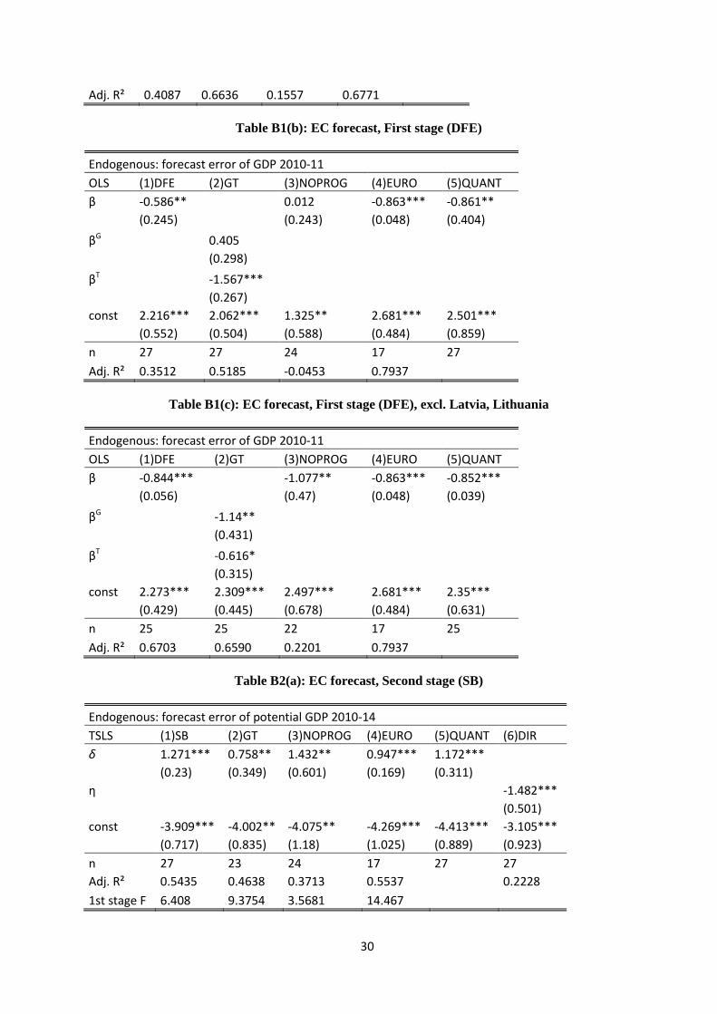
Using European Commission Data

Is the IMF forecast a special case? We test the European Commission’s forecast as well, using the

spring 2010 European Economic Forecast as well as t+4 forecasts of potential output. The EC data

include the whole EU27 and thus some additional Eastern European countries, that are absent from the

IMF dataset. Repeating the previous regressions with EC data, most of the results are confirmed.

Results are shown in Appendix B. Estimates using the structural balance are even more robust to the

perturbations we tested for the IMF data. Concerning the DFE there are two interesting and plausible

outliers: for the whole EU27, the coefficients of interest are somewhat weaker (𝛽𝛽 = [. 5; .7],𝛿𝛿 =

[.9; 1.1]). Most notably, the relation completely diminishes when excluding the program countries

(Table B1(b), Column(3)), and the separate effects of spending and revenue shocks is turned upside

down (Table B1(b), Column(2)). These findings are fully driven by the data of Latvia and Lithuania,

countries that are absent in the IMF dataset and that witnessed a tremendous crash in 2009 with a

cumulated GDP growth forecast error for the years 2008-09 as of the 2008 spring forecast of more

than −20 pp each. It is not implausible that (potential) growth forecasts where more on the pessimistic

13

side in the following years. Moreover, both countries are very small, very open economies that joined

the EU only in 2004, which gave them a strong push to export growth. In such circumstances fiscal

devaluation is considered less harmful (Perotti 2011). When we exclude these special cases, the

previous results of the IMF sample are reestablished in full (Series (c) of Tables B1-4, Appendix B).

Extending the Time Dimension

In our baseline we derive forecast errors from the vintage of spring 2016 vis-à-vis 2010 and are

therefore restricted to only 21 / 22 observations in the IMF case and 27 with EC data. Fiscal

consolidation in many European countries has, however, continued after 2011. Also, it might be

interesting to check the short and long run impact for late crisis years. Therefore, we test for forecasts

in subsequent years and extend the time dimension of the estimation in two ways. First, we assess

different forecast vintages individually in form of a moving window and second, jointly in a panel

structure. As we only have limited access to IMF vintages with t+5 forecasts we concentrate in the

main body of this paper on results with EC data for the moving window and panel model exercise.

Appendix B presents limited samples with IMF data. Generally, the results for the first and second

stage are robust to the exercise of extending the time dimension when using the DFE as fiscal shocks,

while using SB produces rather inconsistent results. The model for the moving window is equivalent

to section 2. The two-year fiscal shocks and growth forecast errors move along with the respective

vintage year. Table 5(a) and (b) and Table 6(a) and (b) show moving window regression results for

vintages between 2010 and 2014 using SB and DFE for the first and second stage, respectively.

[Table 5(a) about here]

[Table 5(b) about here]

[Table 6(a) about here]

[Table 6(b) about here]

In the first stage SB case, baseline results are not confirmed by other vintage years, β becomes

economically and statistically insignificant. However, using DFE provides robust results for the main

period of European consolidation, vintage years 2010 -12 with a multiplier underestimation between -

0.53 and -0.61. Afterwards the effect vanishes, which may be due to the slowdown of consolidation in

14

general, the fact that forecasters learned from their mistakes or be interpreted in line with findings of

regime-dependent multiplier effects (Auerbach and Gorodnichenko 2012, Baum et al. 2012). Turning

to the second stage provides a similar picture. The baseline persistence is qualitatively confirmed for

DFE while SB only yields mixed results. For the years 2010-12, persistence estimated using DFE is on

a somewhat higher level compared to baseline, δ increases from 0.965 for 2010 to 1.394 for 2012,

afterwards fiscal shocks show no significant persistence effect. Hence, we observe a weakening of the

effects in late crisis years. Contrary to baseline estimates, the results for later vintages do not

elementarily differ when excluding Latvia and Lithuania.

In a next step we increase the number of observations by applying a panel structure with different

sets of vintages, following BL in the case of short-term multipliers. The estimation procedure is

analogous to the TSLS estimation described in section two but features a time-fixed effect. The panel

model has the following properties for the first (6) and the second stage (7)13,

∆𝑌𝑌�𝑖𝑖,𝑡𝑡:𝑡𝑡+1𝑓𝑓𝑓𝑓 = 𝛼𝛼 + 𝜌𝜌𝑡𝑡 + 𝛽𝛽Δ𝐹𝐹𝑖𝑖,𝑡𝑡:𝑡𝑡+1|𝑡𝑡

𝑓𝑓 (6)

∆Pot𝑌𝑌𝑖𝑖,𝑡𝑡:𝑡𝑡+5𝑓𝑓𝑓𝑓 = 𝛾𝛾 + 𝜌𝜌𝑡𝑡 + 𝛿𝛿∆𝑌𝑌�𝑖𝑖,𝑡𝑡:𝑡𝑡+1

𝑓𝑓𝑓𝑓 (+𝑋𝑋𝑖𝑖𝜋𝜋) + ω𝑖𝑖,𝑡𝑡:𝑡𝑡+1|𝑡𝑡 (7)

with 𝜌𝜌𝑡𝑡 as a vector of time-fixed effects and t = 2010, … , 2013.

The panel results (Table 7-10) generally confirm the baseline estimates. Again, DFE proofs to be

quite robust for alternative time dimensions, while SB remains ambiguous. The coefficient β stays

within the range of 0.4 to 0.6, see Table 7b. Column 10/11 presents results for a panel estimation

including vintage years 2010 and 2011, column 10/12 the years 2010, 2011 and 2012, and so on.

Including late crisis years somewhat lowers β but the structural underestimation does not vanish.

Coefficient 𝛿𝛿 (Table 8b) on the contrary increases with time, from 1.0 (10/11) to 1.2 (10/14). Even

though 𝛿𝛿 shows a similar development for SB, results are not to be trusted given the insignificant first

stage results. Nonetheless, panel samples using SB shocks starting already in 2009 deliver more robust

estimates but on a somewhat lower level regarding the underestimation of short-run effects, see Table

9. Also note that further specifications with different panel dimensions14 after the crisis for both the

SB and DFE case do not alter the general picture drawn so far – quite robust estimates with general

13 For estimation we use the STATA command “ivreg2” by Baum et al. (2010) with robust standard errors. 14 The panel sample might start later or be shortened, e.g. 11/12-11/14, 12/13 etc.

15

weakening of the baseline effects in later crisis years, in line with the slowdown of consolidation,

potential learning effects or the end of the downturn regime.

[Table 7(a) about here]

[Table 7(b) about here]

[Table 8(a) about here]

[Table 8(b) about here]

[Table 9 about here]

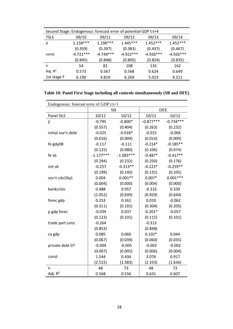
Lastly, we test how our panel results change when the control variables from above are included.

Table 10 presents the underestimation of multiplier effects including all controls simultaneously.

Estimates with DFE are very robust to this exercise. Findings for the second stage including control

variables show similar characteristics, Table 11 – 𝛿𝛿 remains robust to the controls for DFE, while it

does not for SB.

5. Concluding remarks

By exploiting forecast errors of output and long-term potential output growth in the style of

Blanchard and Leigh (2013) and Fatas and Summers (2016), but using a superior, narratively-

identified measure of the fiscal stance, we have investigated as to whether the size and persistence of

fiscal multipliers was underestimated for the austerity measures that were implemented in Europe after

2009. In line with these earlier papers, we find that multipliers were high, in a range of 1.2-1.5, and,

most interestingly, had a permanent effect in the 2010-11 period. These results hold up to a battery of

perturbations and particularly so when relying on our improved identification strategy. Interestingly, it

turns out that the effects weaken for measures in late crisis years and when including very small very

open economies.

In general, we find evidence for strong hysteresis effects as opposed to the short-run pain, long-

term gain consensus that emerged after the early crisis years. That is, the turn to belt tightening was

badly timed and therefore much more costly in terms of long-term output loss than a more gradual,

backloaded consolidation.

16

References

Alesina, A. / Ardagna, S. (2010), Large changes in fiscal policy: taxes versus spending. NBER/Tax Policy & the Economy, 24(1). S. 35–68.

Baum, C.F. / Schaffer, M.E. / Stillman, S. (2010), ivreg2: Stata module for extended instrumental variables/2SLS, GMM and AC/HAC, LIML and k-class regression. http://ideas.repec.org/c/boc/bocode/s425401.html

Blanchard, O. J. / Leigh, D. (2013), Growth forecast errors and fiscal multipliers. NBER Working Paper 18779.

Bom, P. R. / Ligthart, J. E. (2014), What Have We Learned From Three Decades Of Research On The Productivity Of Public Capital? Journal of Economic Surveys, 28(5). S. 889–916.

Born, B. / Müller, G. J. / Pfeiffer, J. (2015), Does austerity pay off? CEPR Discussion Papers, Nr. 10425

Carnot, N. / Castro, F. de (2015), The Discretionary Fiscal Effort: an Assessment of Fiscal Policy and its Output Effect. European Economy Economic Papers, Nr. 543.

Cottarelli, C. / Jaramillo, L. (2012), Walking Hand in Hand: Fiscal Policy and Growth in Advanced Economies. IMF Working Paper, Nr. WP/12/137.

DeLong, J. B. / Summers, L. H. (2012), Fiscal Policy in a Depressed Economy. Brookings Papers on Economic Activity, 2012(1). S. 233–274.

European Commission (2013), Report on Public finances in EMU. European Economy 4|2013.

Fatás, A. (2000), Do business cycles cast long shadows? Short-run persistence and economic growth. Journal of Economic Growth, 5. S. 147–162.

Fatàs, A. / Summers, L. H. (2016), The permanent effects of fiscal consolidations. NBER Working Paper 22374.

Firstrun Project (2016), A dataset of fiscal variables. A vintage of the Ameco database of the European Commission.

Furman, J. (2016), The new view of fiscal policy and its application. Delivery for Conference: Global Implications of Europe’s Redesign. October 5, 2016. New York.

Frankel, J. (2011), Over-optimism in forecasts by official budget agencies and its implications. Oxford Review of Economic Policy, 27(4). S. 536–562.

Gechert, S. (2015), What fiscal policy is most effective? A meta-regression analysis. Oxford Economic Papers, 67(3). S. 553–580.

Gechert, S. / Rannenberg, A. (2017), Which fiscal multipliers are regime-dependent? A meta-regression analysis. Journal of Economic Surveys(forthcoming). Gechert, S. / Rietzler, K. / Tober, S. (2015), The European Commission’s new NAIRU: Does it deliver? Applied Economics Letters, 23(1). S. 6–10.

Hebous, S. (2011), The Effects of Discretionary Fiscal Policy on Macroeconomic Aggregates: A Reappraisal. Journal of Economic Surveys, 25(4). S. 674–707.

IWH (2015), Ökonomische Wirksamkeit der Konjunktur stützenden finanzpolitischen Massnahmen der Jahre 2008 und 2009. IWH Online 4/2015. PROJEKT-NR.: FE 4/12.

17

Jonung, L. / Larch, M. (2006), Improving fiscal policy in the EU: the case for independent forecasts. Economic Policy, 21(47). S. 491–534.

Koo, R. C. (2013), Balance sheet recession as the ‘other half’ of macroeconomics. European Journal of Economics and Economic Policies: Intervention, 10(2). S. 136–157.

Laeven, L. / Valencia, F. (2012), Systemic Banking Crises Database: An Update, IMF Working Paper 12/163.

Logeay, C. / Tober, S. (2006), Hysteresis and the NAIRU in the Euro Area. Scottish Journal of Political Economy, 53(4). S. 409–429.

Mineshima, A. / Poplawski-Ribeiro, M. / Weber, A. (2014), Size of Fiscal Multipliers. C. Cottarelli / P. Gerson / A. Senhadji (Hrsg.), Post-crisis Fiscal Policy. Cambridge Mass.: MIT Press. S. 315–372.

Perotti, R. (2011), The ``Austerity Myth'': Gain Without Pain? NBER working paper, Nr. 17571.

Projektgruppe Gemeinschaftsdiagnose (2009), Im Sog der Weltrezession. In: ifo Schnelldienst 62 (08), 2009, 03-81.

Projektgruppe Gemeinschaftsdiagnose (2010), Erholung setzt sich fort - Risiken bleiben groß. In: ifo Schnelldienst Jahrgang 63, H. 8, 3-78.

Rogoff, K. S. (2012), Austerity and Debt Realism. Project Syndicate, June 1, 2012.

Schäuble, W. (2010), A plan to tackle Europe's debt mountain. Europe's World. October 1, 2010. http://europesworld.org/2010/10/01/a-plan-to-tackle-europes-debt-mountain/

Sturn, S. (2014), Macroeconomic policy in recessions and unemployment hysteresis. Applied Economics Letters, 21(13). S. 914–917.

Trichet, J.-C. (2010), Stimulate no more - it is now time for all to tighten. Financial Times. July 22, 2010. http://www.ft.com/cms/s/0/1b3ae97e-95c6-11df-b5ad-00144feab49a.html

Woodford, M. (2011), Simple Analytics of the Government Expenditure Multiplier. American Economic Journal: Macroeconomics, 3(1). S. 1–35.

18

Appendix A – Computing forecast errors

For the calculation of real GDP and potential GDP growth forecast errors we follow the approach

of FS. The main issue is to make the data for GDP or potential GDP comparable between the different

vintages. The problem is caused by “data revisions, changes in base year and also changes in national

accounting rules” (FS; p. 31). Real GDP growth forecast errors are defined as follows:

∆𝑌𝑌𝑖𝑖,𝑡𝑡:𝑡𝑡+1𝑓𝑓𝑓𝑓 ≡ ∆𝑌𝑌𝑖𝑖,𝑡𝑡:𝑡𝑡+1 − ∆𝑌𝑌𝑖𝑖,𝑡𝑡:𝑡𝑡+1|𝑡𝑡

𝑓𝑓 ,

with ∆𝑌𝑌𝑖𝑖,𝑡𝑡:𝑡𝑡+1𝑓𝑓𝑓𝑓 growth forecast error of real GDP for the years t to t+1 for country i, 𝑌𝑌 actual GDP at

the latest vintage and 𝑌𝑌𝑓𝑓 its respective forecasted value at vintage year t. Hence, the forecast error of

GDP growth is given by the difference between current-vintage figures of the cumulated change in

GDP over two years and its forecast in the spring vintage of year t. In all cases, current-vintage figures

are taken from the spring 2016 publication of either the IMF WEO or the European Commission

Economic Forecast. In order to account for base-year revisions or changes in national accounting rules

that would bias our estimate of the forecast error, we rebase both real GDP level series at t-1, where t

is the year of the earlier vintage. That is, we create two indices for real GDP Y, first for the 2010

vintage and second for the 2016 vintage, and use 2009 as base year (=100) for both series such that

any technical level revisions are ruled out and we can simply compare the subsequent growth. Note

that if we would analyze the 2011 vintage, our base year would be 2010 and so on. Afterwards, we

simply derive the forecast error in our example with

∆𝑌𝑌𝑖𝑖,2010:2011𝑓𝑓𝑓𝑓,2010 = 𝑌𝑌𝑖𝑖,2009:2011

2016 − 𝑌𝑌𝑖𝑖,2009:20112010

𝑌𝑌𝑖𝑖,2009:20112010 ∙ 100.

Turning to potential output (𝑃𝑃𝑐𝑐𝑃𝑃𝑌𝑌), given our interest in 5-year growth rate forecast errors for

potential output we define them as follows:

∆𝑃𝑃𝑐𝑐𝑃𝑃𝑌𝑌𝑖𝑖,𝑡𝑡:𝑡𝑡+5𝑓𝑓𝑓𝑓 ≡ ∆𝑃𝑃𝑐𝑐𝑃𝑃𝑌𝑌𝑖𝑖,𝑡𝑡:𝑡𝑡+5

− ∆𝑃𝑃𝑐𝑐𝑃𝑃𝑌𝑌𝑖𝑖,𝑡𝑡:𝑡𝑡+5|𝑡𝑡𝑓𝑓 .

When computing forecast errors for potential output the values of the different vintages have to be

adjusted in a slightly different way because as new (disappointing) GDP data come in, the assessment

of past potential output values is revised (downwards) as well. Simply comparing cumulated potential

growth rates of different vintages would therefore unduly downplay the forecast error. However, we

19

still want to get rid of technical revisions due to changes in definitions or base years. We compute the

t+5 potential output growth forecast error of the 2010 vintage as

∆𝑃𝑃𝑐𝑐𝑃𝑃𝑌𝑌𝑖𝑖,2010:2015𝑓𝑓𝑓𝑓,2010 = 𝑃𝑃𝑃𝑃𝑡𝑡𝑌𝑌𝑖𝑖,2015

2016 − 𝑃𝑃𝑃𝑃𝑡𝑡𝑌𝑌𝑖𝑖,20152010 ∙𝑘𝑘

𝑃𝑃𝑃𝑃𝑡𝑡𝑌𝑌𝑖𝑖,20152010 ∗𝑘𝑘

∙ 100,

with 𝑘𝑘 being an adjustment factor, given by

𝑘𝑘 = 𝑌𝑌𝑖𝑖,20092016

𝑌𝑌𝑖𝑖,20092010 .

That is, we adjust the potential output forecasts at vintage t by multiplying them with the ratio of

the actual level GDP of t-1 divided by the level of GDP of t-1 at vintage t, thus correcting for any

technical level revisions while acknowledging revisions of past potential output due to growth

disappointments. Note that in the case of potential output we have t+5 forecasts only for IMF data.

The EC forecasts only incorporate figures up to t+4. This caveat has to be considered when comparing

the results for the IMF and the EC case in section 4.

Appendix B

This appendix discloses further robustness tests for our regressions. First, we repeat the exercises of

Tables 1-4, this time for European Commission Economic Forecast data of spring 2010 against spring

2016. Again, we use both the SB (this time from the European Commission) and the DFE measure.

Tables B1-B4 display the findings.

[Table B1(a) about here]

[Table B1(b) about here]

[Table B1(c) about here]

[Table B2(a) about here]

[Table B2(b) about here]

[Table B2(c) about here]

[Table B3(a) about here]

[Table B3(b) about here]

[Table B3(c) about here]

[Table B4(a) about here]

20

[Table B4(b) about here]

[Table B4(c) about here]

In general, the results are confirmed. The effects based on SB (series (a)) are even more robust

when using the EC forecasts. However, when including all 27 EU countries the effects weaken

somewhat for the DFE measure (series (b)): they do not hold when excluding Greece, Portugal and

Ireland (Table B1(b), column (3)); moreover, the earlier finding that underestimation of multipliers

was stronger for spending side-measures is turned upside down. These changes very much depend on

the inclusion of Latvia and Lithuania. Series (c) of Tables B1-B4 gives the findings based on DFE for

a sample excluding these two observations: all previous results are reconfirmed.

Table B5 presents moving window estimations with IMF data, showing a very similar picture for

the two years of available vintages compared to the EC data case. DFE shocks indicate to have a

weakening effect on the coefficients in the first and second stage, while first stage SB estimations are

only significant in the 2010 baseline. The second stage for SB looks comparatively good, but cannot

be relied upon given the opaque first stage results.

Table B6a and b include panel specifications with available IMF data, confirming previous results.

[Table B5 about here]

[Table B6(a) about here]

[Table B6(b) about here]

21

Figures and Tables

Figure 1: Vintages of GDP growth rate forecasts for the EU-27 and Greece, in %, 2007-2016

EU-27 Greece

Source: Ameco, Firstrun database “A dataset of fiscal variables”, own illustration.

Figure 2: Vintages of potential GDP growth rate forecasts for the EU-27 and Greece, in %,

2007-2016

EU-27 Greece

Source: Ameco, Firstrun database “A dataset of fiscal variables”, own illustration.

-5

-4

-3

-2

-1

0

1

2

3

4

2007 2008 2009 2010 2011 2012 2013 2014 2015 2016

2008 Autumn 2009 Autumn2010 Autumn 2011 Autumn2012 Autumn 2013 Autumn2014 Autumn 2015 Autumn

-10

-8

-6

-4

-2

0

2

4

6

2007 2008 2009 2010 2011 2012 2013 2014 2015 2016

2008 Autumn 2009 Autumn2010 Autumn 2011 Autumn2012 Autumn 2013 Autumn2014 Autumn 2015 Autumn

0

1

1

2

2

3

2007 2008 2009 2010 2011 2012 2013 2014 2015 2016

2008 Autumn 2009 Autumn2010 Autumn 2011 Autumn2012 Autumn 2013 Autumn2014 Autumn 2015 Autumn

-5

-4

-3

-2

-1

0

1

2

3

4

5

2007 2008 2009 2010 2011 2012 2013 2014 2015 2016

2008 Autumn 2009 Autumn2010 Autumn 2011 Autumn2012 Autumn 2013 Autumn2014 Autumn 2015 Autumn

22

Table 1(a): First stage: Underestimation of multipliers with structural balance (SB)

Endogenous: forecast error of GDP 2010-11 OLS (1)SB (2)GT (3)NOPROG (4)ADVA (5)EURO (6)QUANT β -1.341** -0.942*** -0.632 -1.534** -1.272***

(0.53)

(0.243) (0.614) (0.578) (0.306)

βG

-1.699***

(0.477)

βT

-0.967**

(0.371)

const 1.15*** 1.223*** 1.101*** 0.919* 1.34*** 0.856

(0.402) (0.36) (0.374) (0.493) (0.393) (0.62)

n 22 22 19 31 14 22 Adj. R² 0.4755 0.6024 0.3307 0.0749 0.5763

Table 1(b): First stage: Underestimation of multipliers with discretionary fiscal effort (DFE)

Endogenous: forecast error of GDP 2010-11 OLS (1)DFE (2)GT (3)G (4)T (5)NOPROG (6)EURO (7)QUANT β -0.861*** -0.934* -0.875*** -0.874***

(0.055)

(0.498) (0.052) (0.055)

βG

-0.928 -1.906***

(0.761) (0.209)

βT

-0.812

-1.462***

(0.566)

(0.122)

const 2.75*** 2.761*** 2.84*** 2.552*** 2.7*** 2.835*** 2.573***

(0.489) (0.516) (0.553) (0.522) (0.713) (0.573) (0.669)

n 21 21 21 21 18 16 21 Adj. R² 0.6983 0.6816 0.6639 0.6721 0.1306 0.7508

Table 2(a): Second Stage: Persistence of multiplier effects (SB)

Endogenous: forecast error of potential GDP 2010-15 TSLS (1)SB (2)GT (3)NOPROG (4)EURO (5)QUANT (6)DIR δ 1.005** 1.046*** 1.296** 1.065*** 1.401**

(0.402) (0.289) (0.544) (0.387) (0.647) η

-1.348

(1.013)

const -3.521**

-3.537*** -4.016**

-3.548*** -3.834**

-2.365**

(0.869) (0.819) (0.861) (1.114) (1.356) (1)

n 22 22 19 14 22 22 Adj. R² 0.5813 0.5813 0.3346 0.6866

0.1218

1st stage F 6.3952 6.3621 15.036 7.0449

23

Table 2(b): Second Stage: Persistence of multiplier effects (DFE)

Endogenous: forecast error of potential GDP 2010-15 TSLS (1)DFE (2)GT (3)NOPROG (4)EURO (5)QUANT (6)DIR δ 1.236*** 1.234*** 1.319* 1.28*** 1.216***

(0.072) (0.073) (0.689) (0.086) (0.233) η

-1.065***

(0.1)

const -3.914*** -3.912*** -4.459* -3.303*** -4.304*** -0.515

(0.745) (0.747) (1.523) (0.872) (0.704) (1.257)

n 21 21 18 16 21 21 Adj. R² 0.6807 0.6807 0.6109 0.7303

0.3203

1st stage F 244.36 115.39 3.5254 279.43

Table 3(a): First stage with controls (SB)

additional control X β θ const n Adj. R² (1) fe gdp0709 -1.316(0.516)** 0.043(0.143) 1.451(0.915) 22 0.451 (2) forec gdp1011 -1.174(0.442)** 0.242(0.238) 0.409(0.842) 22 0.473 (3) fe sb1011 -1.161(0.427)** -0.51(0.365) 1.553(0.582)** 22 0.501 (4) trade part cons -1.402(0.488)*** 2.321(1.695) 0.964(0.419)** 22 0.509 (5) sov'n debt09 -1.29(0.507)** -0.008(0.018) 1.632(1.284) 22 0.451 (6) sb09 -1.095(0.621)* 0.141(0.248) 1.689(1.131) 22 0.454 (7) sov'n cds10q1 -1.199(0.587)* -0.003(0.006) 1.408(0.639)** 22 0.457 (8) bankcrisis -1.324(0.515)** -0.268(0.881) 1.262(0.481)** 22 0.450 (9) private debt 07 -1.312(0.557)** 0(0.008) 1.107(0.955) 21 0.433

(10) ca07 -1.301(0.685)* 0.013(0.087) 1.143(0.395)*** 22 0.448

Table 3(b): First stage with controls (DFE)

additional control X β θ const n Adj. R² (1) fe gdp0709 -0.861(0.06)*** -0.06(0.103) 2.186(1.038)** 21 0.693 (2) forec gdp1011 -0.864(0.139)*** -0.005(0.305) 2.77(1.195)** 21 0.682 (3) fe sb1011 -0.906(0.11)*** 0.263(0.326) 2.35(0.473)*** 19 0.733 (4) trade part cons -0.857(0.051)*** 2.12(0.686)*** 2.557(0.465)*** 21 0.725 (5) sov'n debt09 -0.806(0.084)*** -0.015(0.018) 3.507(1.183)*** 21 0.695 (6) sb09 -0.803(0.138)*** 0.043(0.198) 2.563(0.812)*** 19 0.725 (7) sov'n cds10q1 -0.966(0.336)** 0.007(0.018) 2.344(0.949)** 20 0.680 (8) bankcrisis -0.85(0.053)*** -0.72(0.85) 3.068(0.686)*** 21 0.694 (9) private debt 07 -0.876(0.061)*** -0.004(0.006) 3.17(1.004)*** 20 0.703

(10) ca07 -0.924(0.125)*** -0.05(0.094) 2.787(0.525)*** 21 0.690

24

Table 4(a): Second stage with controls (SB)

additional control X δ π const n Adj. R² 1st F (1) fe gdp0709 0.845(0.406)** 0.374(0.263) -0.715(1.792) 22 0.575 3.327 (2) forec gdp1011 1.382(0.403)*** -0.729(0.275)*** -1.72(1.102) 22 0.684 3.611 (3) fe sb1011 1.043(0.508)** 0.145(0.636) -3.679(1.209)*** 22 0.571 4.029 (4) trade part cons 1.135(0.276)*** 6.628(1.59)*** -4.203(0.598)*** 22 0.708 5.004 (5) sov'n debt09 1.124(0.472)** 0.025(0.036) -5.156(2.78)* 22 0.590 3.252 (6) sb09 1.567(0.699)** -0.432(0.54) -5.816(3.004)* 22 0.625 2.997 (7) sov'n cds10q1 0.962(0.605) -0.001(0.01) -3.364(1.713)** 22 0.550 3.328 (8) bankcrisis 1.083(0.37)*** 1.625(1.41) -4.291(1.199)*** 22 0.595 3.620 (9) private debt 07 0.763(0.456)* 0.027(0.015)* -7.345(1.682)*** 21 0.659 2.783

(10) ca07 0.744(0.76) 0.111(0.166) -3.286(0.986)*** 22 0.505 3.541

Table 4(b): Second stage with controls (DFE)

additional control X δ π const n Adj. R² 1st F (1) fe gdp0709 1.236(0.074)*** -0.023(0.121) -4.131(1.44)*** 21 0.663 103.67 (2) forec gdp1011 1.651(0.201)*** -0.859(0.369)** -1.731(1.251) 21 0.771 115.65 (3) fe sb1011 1.312(0.189)*** 0.381(0.537) -4.582(0.805)*** 19 0.635 88.94 (4) trade part cons 1.22(0.092)*** 6.582(1.605)*** -4.469(0.548)*** 21 0.780 143.76 (5) sov'n debt09 1.297(0.144)*** 0.014(0.029) -4.799(2.018)** 21 0.677 128.32 (6) sb09 1.808(0.263)*** -0.727(0.297)** -8.094(1.738)*** 19 0.755 91.09 (7) sov'n cds10q1 1.263(0.737)* 0.003(0.036) -4.404(3.956) 20 0.660 97.64 (8) bankcrisis 1.286(0.099)*** 2.709(1.481)* -5.249(1.1)*** 21 0.732 148.98 (9) private debt 07 1.12(0.083)*** 0.019(0.016) -6.542(1.552)*** 20 0.742 122.66

(10) ca07 1.331(0.13)*** -0.065(0.096) -4.128(0.707)*** 21 0.678 130.57

Table 5(a): Moving Window First Stage (SB)

Endogenous: forecast error of GDP t:t+1 OLS 2010 2011 2012 2013 2014 β -1.166** 0.065 -0.473 0.564 0.204

(0.461) (0.268) (0.312) (0.389) (0.578)

const 0.633 -2.916*** -0.876 0.584 0.649

(0.500) (0.847) (0.554) (0.571) (0.526) n 27 27 27 27 27 Adj. R² 0.431 0.001 0.094 0.065 0.009

25

Table 5(b): Moving Window First Stage (DFE)

Endogenous: forecast error of GDP t:t+1 OLS 2010 2011 2012 2013 2014 β -0.586** -0.609** -0.530*** 0.248 0.343

(0.245) (0.252) (0.116) (0.172) (0.286)

const 2.216*** -1.057 -0.029 0.474 0.417

(0.552) (0.851) (0.460) (0.570) (0.516) n 27 27 27 27 27 Adj. R² 0.376 0.308 0.440 0.056 0.030

Table 6(a): Moving Window Second Stage (SB)

Endogenous: forecast error of potential GDP t:t+4 TSLS 2010 2011 2012 2013 2014 δ 1.271*** -0.087 2.877*** 1.379 1.445

(0.222) (5.688) (1.095) (1.279) (2.223)

const -3.909*** -3.359 3.921** 0.601 0.401 (0.690) (15.840) (1.836) (0.978) (1.518) n 27 27 27 27 27 Adj. R² 0.543 -0.126 0.186 0.658 0.729 1st stage F 6.408 0.0594 2.290 2.101 0.124

Table 6(b): Moving Window Second Stage (DFE)

Endogenous: forecast error of potential GDP t:t+4 TSLS 2010 2011 2012 2013 2014 δ 0.965*** 0.983*** 1.394*** 0.893 -0.242

(0.257) (0.190) (0.298) (1.245) (1.152)

const -3.675*** -0.312 1.731* 1.031 1.449

(0.690) (0.913) (0.965) (1.159) (1.342) n 27 27 27 27 27 Adj. R² 0.514 0.522 0.486 0.504 -0.305 1st stage F 5.708 5.826 20.75 2.077 1.439

Table 7(a): Panel First Stage (SB)

Endogenous: forecast error of GDP t:t+1 Panel OLS 10/11 10/12 10/13 10/14 β -0.574 -0.547** -0.419* -0.341

(0.349) (0.269) (0.249) (0.233)

const 0.702 0.705 0.719 0.728

(0.544) (0.541) (0.560) (0.573) n 54 81 108 135 Adj. R² 0.283 0.249 0.248 0.223

26

Table 7(b): Panel First Stage (DFE)

Endogenous: forecast error of GDP t:t+1 Panel OLS 10/11 10/12 10/13 10/14 β -0.596*** -0.577*** -0.456*** -0.419***

(0.174) (0.132) (0.143) (0.145)

const 2.240*** 2.192*** 1.894*** 1.803***

(0.516) (0.481) (0.494) (0.495) n 54 81 108 135 Adj. R² 0.476 0.468 0.380 0.326

Table 8(a): Panel Second Stage (SB)

Endogenous: forecast error of potential GDP t:t+4 Panel TSLS 10/11 10/12 10/13 10/14 δ 1.345*** 1.695*** 1.744*** 1.766***

(0.363) (0.444) (0.565) (0.637)

const -3.966*** -4.235*** -4.273*** -4.290***

(0.735) (0.864) (0.934) (0.977) n 54 81 108 135 Adj. R² 0.540 0.503 0.582 0.608 1st stage F 2.705 4.125 2.841 2.142

Table 8(b): Panel Second Stage (DFE)

Endogenous: forecast error of potential GDP t:t+4 Panel TSLS 10/11 10/12 10/13 10/14 δ 0.973*** 1.086*** 1.101*** 1.152***

(0.162) (0.139) (0.175) (0.189)

const -3.681*** -3.768*** -3.779*** -3.818***

(0.689) (0.674) (0.676) (0.674) n 54 81 108 135 Adj. R² 0.519 0.531 0.586 0.618 1st stage F 11.72 19.19 10.13 8.396

Table 9: Further Panels First and Second Stage (SB)

First Stage: Endogenous: forecast error of GDP t:t+1 OLS 09/10 09/11 09/12 09/13 09/14 β -0.631** -0.470** -0.471** -0.401** -0.354**

(0.253) (0.214) (0.188) (0.179) (0.173)

const -0.228 0.007 0.007 0.109 0.178

(0.741) (0.719) (0.700) (0.697) (0.696)

n 54 81 108 135 162 Adj. R² 0.155 0.252 0.242 0.228 0.205

27

Second Stage: Endogenous: forecast error of potential GDP t:t+4 TSLS 09/10 09/11 09/12 09/13 09/14 δ 1.158*** 1.198*** 1.445*** 1.452*** 1.452***

(0.359) (0.397) (0.383) (0.437) (0.467)

const -4.721*** -4.749*** -4.922*** -4.926*** -4.926***

(0.845) (0.848) (0.805) (0.824) (0.835) n 54 81 108 135 162 Adj. R² 0.573 0.567 0.568 0.624 0.649 1st stage F 6.190 4.819 6.269 5.013 4.211

Table 10: Panel First Stage including all controls simultaneously (SB and DFE)

Endogenous: forecast error of GDP t:t+1 SB DFE Panel OLS 10/11 10/12 10/11 10/12 β -0.795 -0.800* -0.877*** -0.734***

(0.557) (0.404) (0.263) (0.232)

initial sov'n debt -0.025 -0.018* -0.015 -0.004

(0.016) (0.009) (0.014) (0.009)

fe gdp08 -0.117 -0.111 -0.214* -0.185**

(0.125) (0.080) (0.106) (0.074)

fe sb -1.177*** -1.083*** -0.487* -0.417**

(0.294) (0.232) (0.250) (0.176)

init sb -0.257 -0.313** -0.223* -0.259**

(0.199) (0.140) (0.131) (0.105)

sov'n cds10q1 0.004 0.001** 0.007* 0.001***

(0.004) (0.000) (0.004) (0.000)

bankcrisis 0.488 0.957 -0.316 0.339

(1.052) (0.699) (0.929) (0.644)

forec gdp 0.253 0.161 0.010 -0.062

(0.311) (0.191) (0.304) (0.205)

p gdp forec -0.039 0.037 -0.201* -0.057

(0.123) (0.101) (0.115) (0.101)

trade part cons -0.264

-0.313

(0.853)

(0.848)

ca gdp 0.085 0.060 0.102* 0.044

(0.067) (0.039) (0.060) (0.035)

private debt 07 -0.004 -0.005 -0.003 -0.002

(0.007) (0.005) (0.006) (0.004)

const 1.544 0.434 3.076 0.917

(2.515) (1.583) (2.333) (1.636)

n 48 73 48 73 Adj. R² 0.568 0.556 0.631 0.607

28

Table 11: Panel Second Stage including all controls simultaneously (SB and DFE)

Endogenous: forecast error of potential GDP t:t+4 SB DFE Panel TSLS 10/11 10/12 10/11 10/12 δ 0.152 0.908* 0.739** 1.134***

(0.728) (0.488) (0.345) (0.367)

initial sov'n debt 0.009 0.031* 0.019 0.034**

(0.022) (0.018) (0.019) (0.017)

fe gdp08 -0.354* -0.270*** -0.262*** -0.237**

(0.194) (0.102) (0.092) (0.092)

fe sb -1.066 0.196 -0.538 0.364

(0.733) (0.459) (0.393) (0.377)

init sb 0.016 -0.211 0.001 -0.203

(0.131) (0.145) (0.106) (0.144)

sov'n cds10q1 0.015*** -0.000 0.013*** -0.001*

(0.005) (0.000) (0.004) (0.000)

bankcrisis 1.767 0.436 1.421 0.164

(1.324) (1.139) (0.917) (1.067)

forec gdp 0.687** 0.148 0.464* 0.081

(0.348) (0.213) (0.241) (0.183)

p gdp forec 0.253 0.302** 0.269** 0.286**

(0.172) (0.142) (0.123) (0.141)

trade part cons 1.512

1.157

(1.136)

(1.158)

ca gdp 0.198* 0.098 0.137 0.082

(0.119) (0.067) (0.089) (0.068)

private debt 07 0.007 0.008 0.006 0.008

(0.008) (0.006) (0.007) (0.006)

const -13.049*** -14.128*** -13.306*** -13.992*** (2.623) (2.957) (2.111) (2.956) n 48 73 48 73 Adj. R² 0.457 0.591 0.685 0.615 1st stage F 2.035 3.927 11.16 10.05

Table B1(a): EC forecast, First stage (SB)

Endogenous: forecast error of GDP 2010-11 OLS (1)SB (2)GT (3)NOPROG (4)EURO (5)QUANT β -1.166** -0.618* -1.676*** -0.966***

(0.461)

(0.327) (0.441) (0.266)

βG

-1.719***

(0.397)

βT

-0.959***

(0.282)

const 0.633 0.895** 1.134** 0.584 0.614

(0.5) (0.392) (0.434) (0.513) (0.637)

n 27 23 24 17 27

29

Adj. R² 0.4087 0.6636 0.1557 0.6771

Table B1(b): EC forecast, First stage (DFE)

Endogenous: forecast error of GDP 2010-11 OLS (1)DFE (2)GT (3)NOPROG (4)EURO (5)QUANT β -0.586** 0.012 -0.863*** -0.861**

(0.245)

(0.243) (0.048) (0.404)

βG

0.405

(0.298)

βT

-1.567***

(0.267)

const 2.216*** 2.062*** 1.325** 2.681*** 2.501***

(0.552) (0.504) (0.588) (0.484) (0.859)

n 27 27 24 17 27 Adj. R² 0.3512 0.5185 -0.0453 0.7937

Table B1(c): EC forecast, First stage (DFE), excl. Latvia, Lithuania

Endogenous: forecast error of GDP 2010-11 OLS (1)DFE (2)GT (3)NOPROG (4)EURO (5)QUANT β -0.844*** -1.077** -0.863*** -0.852***

(0.056)

(0.47) (0.048) (0.039)

βG

-1.14**

(0.431)

βT

-0.616*

(0.315)

const 2.273*** 2.309*** 2.497*** 2.681*** 2.35***

(0.429) (0.445) (0.678) (0.484) (0.631)

n 25 25 22 17 25 Adj. R² 0.6703 0.6590 0.2201 0.7937

Table B2(a): EC forecast, Second stage (SB)

Endogenous: forecast error of potential GDP 2010-14 TSLS (1)SB (2)GT (3)NOPROG (4)EURO (5)QUANT (6)DIR δ 1.271*** 0.758** 1.432** 0.947*** 1.172***

(0.23) (0.349) (0.601) (0.169) (0.311) η

-1.482***

(0.501)

const -3.909*** -4.002** -4.075** -4.269*** -4.413*** -3.105***

(0.717) (0.835) (1.18) (1.025) (0.889) (0.923)

n 27 23 24 17 27 27 Adj. R² 0.5435 0.4638 0.3713 0.5537

0.2228

1st stage F 6.408 9.3754 3.5681 14.467

30

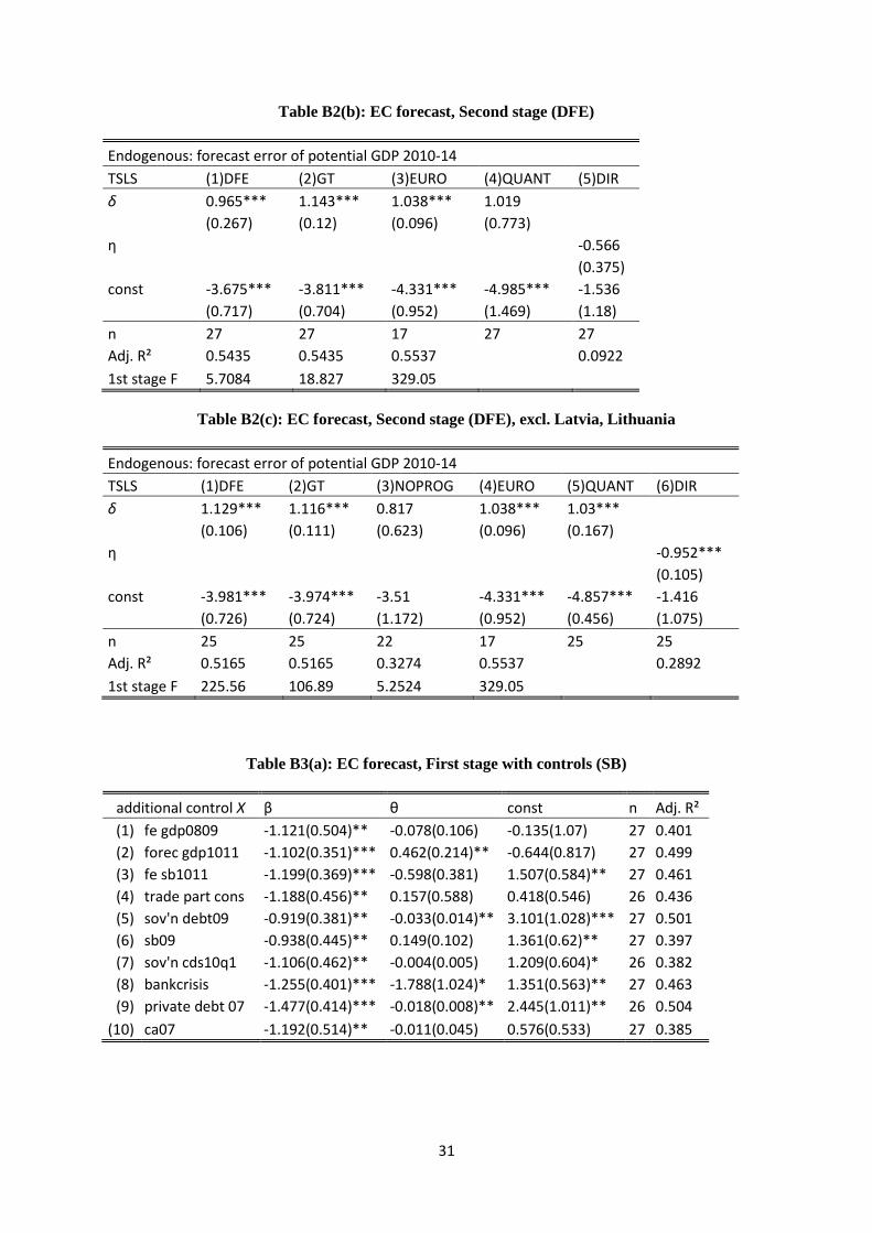
Table B2(b): EC forecast, Second stage (DFE)

Endogenous: forecast error of potential GDP 2010-14 TSLS (1)DFE (2)GT (3)EURO (4)QUANT (5)DIR δ 0.965*** 1.143*** 1.038*** 1.019

(0.267) (0.12) (0.096) (0.773) η

-0.566

(0.375)

const -3.675*** -3.811*** -4.331*** -4.985*** -1.536

(0.717) (0.704) (0.952) (1.469) (1.18)

n 27 27 17 27 27 Adj. R² 0.5435 0.5435 0.5537

0.0922

1st stage F 5.7084 18.827 329.05

Table B2(c): EC forecast, Second stage (DFE), excl. Latvia, Lithuania

Endogenous: forecast error of potential GDP 2010-14 TSLS (1)DFE (2)GT (3)NOPROG (4)EURO (5)QUANT (6)DIR δ 1.129*** 1.116*** 0.817 1.038*** 1.03***

(0.106) (0.111) (0.623) (0.096) (0.167) η

-0.952***

(0.105)

const -3.981*** -3.974*** -3.51 -4.331*** -4.857*** -1.416

(0.726) (0.724) (1.172) (0.952) (0.456) (1.075)

n 25 25 22 17 25 25 Adj. R² 0.5165 0.5165 0.3274 0.5537

0.2892

1st stage F 225.56 106.89 5.2524 329.05

Table B3(a): EC forecast, First stage with controls (SB)

additional control X β θ const n Adj. R² (1) fe gdp0809 -1.121(0.504)** -0.078(0.106) -0.135(1.07) 27 0.401 (2) forec gdp1011 -1.102(0.351)*** 0.462(0.214)** -0.644(0.817) 27 0.499 (3) fe sb1011 -1.199(0.369)*** -0.598(0.381) 1.507(0.584)** 27 0.461 (4) trade part cons -1.188(0.456)** 0.157(0.588) 0.418(0.546) 26 0.436 (5) sov'n debt09 -0.919(0.381)** -0.033(0.014)** 3.101(1.028)*** 27 0.501 (6) sb09 -0.938(0.445)** 0.149(0.102) 1.361(0.62)** 27 0.397 (7) sov'n cds10q1 -1.106(0.462)** -0.004(0.005) 1.209(0.604)* 26 0.382 (8) bankcrisis -1.255(0.401)*** -1.788(1.024)* 1.351(0.563)** 27 0.463 (9) private debt 07 -1.477(0.414)*** -0.018(0.008)** 2.445(1.011)** 26 0.504

(10) ca07 -1.192(0.514)** -0.011(0.045) 0.576(0.533) 27 0.385

31

Table B3(b): EC forecast, First stage with controls (DFE)

additional control X β θ const n Adj. R² (1) fe gdp0809 -0.704(0.158)*** -0.278(0.093)*** -0.265(1.027) 27 0.530 (2) forec gdp1011 -0.566(0.258)** 0.051(0.25) 2.023(1.000)* 27 0.325 (3) fe sb1011 -0.675(0.249)** 0.377(0.539) 1.882(0.621)*** 27 0.346 (4) trade part cons -0.664(0.217)*** -0.061(0.639) 2.165(0.516)*** 26 0.452 (5) sov'n debt09 -0.446(0.218)* -0.035(0.015)** 4.451(1.206)*** 27 0.455 (6) sb09 -0.402(0.307) 0.254(0.143)* 2.952(0.697)*** 27 0.374 (7) sov'n cds10q1 -0.772(0.287)** 0.008(0.01) 1.536(0.724)** 26 0.351 (8) bankcrisis -0.579(0.246)** -0.296(1.001) 2.319(0.74)*** 27 0.326 (9) private debt 07 -0.613(0.248)** -0.006(0.006) 2.902(1.095)** 26 0.337

(10) ca07 -0.604(0.267)** -0.012(0.077) 2.195(0.533)*** 27 0.325

Table B3(c): EC forecast, First stage with controls (DFE), excl. Latvia, Lithuania

additional control X β θ const n Adj. R² (1) fe gdp0809 -0.844(0.059)*** -0.095(0.114) 1.415(1.101) 25 0.673 (2) forec gdp1011 -0.781(0.122)*** 0.167(0.223) 1.644(0.875)* 25 0.666 (3) fe sb1011 -0.83(0.088)*** -0.081(0.397) 2.349(0.53)*** 25 0.656 (4) trade part cons -0.848(0.056)*** -0.248(0.575) 2.327(0.443)*** 25 0.657 (5) sov'n debt09 -0.758(0.077)*** -0.015(0.013) 3.249(1.059)*** 25 0.679 (6) sb09 -0.72(0.083)*** 0.154(0.122) 2.711(0.646)*** 25 0.674 (7) sov'n cds10q1 -0.633(0.091)*** -0.012(0.005)** 3.019(0.548)*** 24 0.702 (8) bankcrisis -0.839(0.064)*** -0.255(0.761) 2.365(0.547)*** 25 0.657 (9) private debt 07 -0.859(0.06)*** -0.004(0.006) 2.665(0.902)*** 24 0.670

(10) ca07 -0.79(0.085)*** 0.049(0.06) 2.359(0.401)*** 25 0.672

Table B4(a): EC forecast, Second stage with controls (SB)

additional control X δ π const n Adj. R² 1st F (1) fe gdp0809 1.234(0.227)*** -0.074(0.136) -4.619(1.878)** 27 0.530 4.52 (2) forec gdp1011 1.299(0.241)*** -0.234(0.282) -3.281(1.066)*** 27 0.534 6.17 (3) fe sb1011 1.262(0.213)*** 0.188(0.506) -4.179(1.298)*** 27 0.527 5.49 (4) trade part cons 1.283(0.222)*** -1.551(1.431) -3.633(0.837)*** 26 0.524 3.41 (5) sov'n debt09 1.43(0.331)*** 0.025(0.024) -5.861(1.795)*** 27 0.540 5.46 (6) sb09 1.19(0.575)** 0.061(0.36) -3.559(2.379) 27 0.525 3.51 (7) sov'n cds10q1 1.406(0.302)*** 0.007(0.008) -4.8(1.635)*** 26 0.532 2.88 (8) bankcrisis 1.258(0.218)*** 0.307(1.272) -4.024(1.128)*** 27 0.525 5.14 (9) private debt 07 1.308(0.223)*** 0.001(0.008) -4.525(1.015)*** 26 0.642 6.71

(10) ca07 1.424(0.304)*** -0.074(0.06) -4.404(0.812)*** 27 0.536 3.24

32

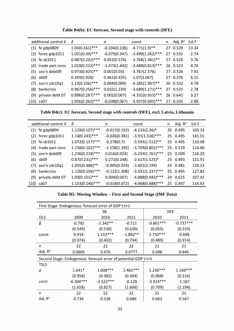
Table B4(b): EC forecast, Second stage with controls (DFE)

additional control X δ π const n Adj. R² 1st F (1) fe gdp0809 1.04(0.161)*** -0.104(0.136) -4.771(1.9)** 27 0.529 13.34 (2) forec gdp1011 1.021(0.39)*** -0.079(0.347) -3.499(1.262)*** 27 0.531 2.74 (3) fe sb1011 0.987(0.242)*** 0.052(0.574) -3.768(1.481)** 27 0.526 3.76 (4) trade part cons 1.019(0.223)*** -1.473(1.442) -3.488(0.813)*** 26 0.523 4.76 (5) sov'n debt09 0.973(0.425)** 0.001(0.03) -3.767(2.376) 27 0.526 7.93 (6) sb09 0.393(0.928) 0.461(0.435) -1.07(3.067) 27 0.376 6.15 (7) sov'n cds10q1 1.13(0.336)*** 0.004(0.009) -4.285(1.907)** 26 0.532 4.78 (8) bankcrisis 0.967(0.256)*** 0.032(1.239) -3.689(1.171)*** 27 0.525 2.78 (9) private debt 07 0.896(0.287)*** 0.002(0.007) -4.331(0.953)*** 26 0.642 3.27

(10) ca07 1.056(0.263)*** -0.038(0.067) -3.937(0.695)*** 27 0.535 2.88

Table B4(c): EC forecast, Second stage with controls (DFE), excl. Latvia, Lithuania

additional control X δ π const n Adj. R² 1st F (1) fe gdp0809 1.129(0.107)*** -0.017(0.192) -4.133(2.26)* 25 0.495 103.33 (2) forec gdp1011 1.14(0.243)*** -0.026(0.381) -3.91(1.516)*** 25 0.495 141.55 (3) fe sb1011 1.072(0.157)*** -0.278(0.7) -3.593(1.512)** 25 0.495 110.08 (4) trade part cons 1.158(0.102)*** -1.558(1.395) -3.709(0.802)*** 25 0.519 114.00 (5) sov'n debt09 1.236(0.218)*** 0.016(0.024) -5.259(1.761)*** 25 0.509 116.29 (6) sb09 0.87(0.231)*** 0.272(0.248) -2.617(1.525)* 25 0.493 121.91 (7) sov'n cds10q1 1.035(0.486)** -0.005(0.024) -3.401(3.199) 24 0.481 120.53 (8) bankcrisis 1.126(0.104)*** -0.122(1.308) -3.931(1.237)*** 25 0.495 127.82 (9) private debt 07 1.09(0.101)*** 0.004(0.007) -4.888(0.943)*** 24 0.625 107.41

(10) ca07 1.153(0.146)*** -0.018(0.072) -4.068(0.688)*** 25 0.497 114.63

Table B5: Moving Window – First and Second Stage (IMF Data)

First Stage: Endogenous: forecast error of GDP t:t+1 SB DFE OLS 2009 2010 2011 2010 2011 β -0.792 -1.342** -0.711 -0.861*** -0.737***

(0.549) (0.530) (0.630) (0.055) (0.219)

const 0.918 1.153*** -1.892** 2.750*** -0.696

(0.974) (0.402) (0.734) (0.489) (0.914)

n 22 22 22 21 21 Adj. R² 0.0605 0.476 0.0777 0.698 0.445 Second Stage: Endogenous: forecast error of potential GDP t:t+5 TSLS δ 1.641* 1.008*** 1.465*** 1.236*** 1.169***

(0.958) (0.382) (0.504) (0.068) (0.216)

const -6.304*** -3.522*** -0.129 -3.914*** -1.187

(1.658) (0.827) (1.606) (0.709) (1.194) n 22 22 22 21 21 Adj. R² 0.734 0.538 0.680 0.663 0.567

33

1st stage F 2.081 6.403 1.272 244.4 11.32

Table B6(a): Panels First Stage (IMF Data)

Endogenous: forecast error of GDP t:t+1 SB DFE Panel - OLS 09/11 10/11 09/11 All controls 10/11 10/11 All controls β -0.988*** -1.063** -1.351*** -0.800*** -0.813***

(0.356) (0.427) (0.459) (0.109) (0.255)

initial sov'n debt

-0.023 0.013

(0.014) (0.017)

fe gdp08

0.485*** 0.529***

(0.094) (0.157)

fe sb

-0.507** 0.032

(0.241) (0.259)

init sb

-0.674*** -0.418*

(0.194) (0.209)

sov'n cds10q1

0.000 0.001

(0.003) (0.004)

bankcrisis

0.234 -0.611

(0.590) (0.948)

forec gdp

-0.395** -0.360*

(0.177) (0.183)

p gdp forec

0.519*** 0.456

(0.141) (0.316)

trade part cons

0.635 1.127

(0.971) (0.685)

ca gdp

0.130** 0.154

(0.057) (0.115)

private debt 07

0.000 0.004

(0.005) (0.006)

const 0.761 0.997** 0.902 2.617*** 0.920

(0.806) (0.431) (1.776) (0.496) (3.323) n 66 44 63 42 36 Adj. R² 0.402 0.431 0.643 0.660 0.806

34

Table B6(b): Panels Second Stage (IMF Data)

Endogenous: forecast error of potential GDP t:t+5 SB DFE TSLS 09/11 10/11 09/11 All controls 10/11 10/11 All controls δ 1.253*** 1.143*** 1.447*** 1.205*** 1.875***

(0.309) (0.280) (0.224) (0.106) (0.234)

initial sov'n debt

-0.000 0.002

(0.016) (0.016)

fe gdp08

0.090 -0.372**

(0.132) (0.156)

fe sb

0.672*** 0.209

(0.205) (0.364)

init sb

-0.436*** -0.426**

(0.133) (0.175)

sov'n cds10q1

0.002 0.003

(0.003) (0.003)

bankcrisis

-0.124 0.697

(0.576) (0.810)

forec gdp

0.108 -0.072

(0.224) (0.186)

p gdp forec

-0.115 -0.286

(0.141) (0.197)

trade part cons

1.511* 0.875

(0.876) (1.112)

ca gdp

0.147** 0.046

(0.074) (0.133)

private debt 07

0.022*** 0.008

(0.005) (0.005)

const -5.702*** -3.576*** -7.731*** -3.886*** -9.549***

(0.981) (0.783) (1.538) (0.736) (1.886)

n 66 44 63 42 36 Adj. R² 0.644 0.611 0.839 0.626 0.800 1st stage F 7.705 6.198 8.656 53.94 10.20

35

Impressum

Publisher: Hans-Böckler-Stiftung, Hans-Böckler-Str. 39, 40476 Düsseldorf, Germany Phone: +49-211-7778-331, IMK@boeckler.de, http://www.imk-boeckler.de

IMK Working Paper is an online publication series available at: http://www.boeckler.de/imk_5016.htm

ISSN: 1861-2199 The views expressed in this paper do not necessarily reflect those of the IMK or the Hans-Böckler-Foundation. All rights reserved. Reproduction for educational and non-commercial purposes is permitted provided that the source is acknowledged.