workshop: opto-acoustics with comsol - cudoscudos.org.au/nusod_tutorial.pdf · workshop:...
TRANSCRIPT
Workshop: Opto-acoustics with COMSOL
Christian Wolff1,3 and Michael J. A. Smith1,2
1. Centre for Ultrahigh bandwidth Devices for Optical Systems (CUDOS),2. Institute of Photonics and Optical Science (IPOS), School of Physics, University of
Sydney,3. School of Mathematical and Physical Sciences, University of Technology Sydney
July 15, 2016
C. Wolff & M. J. A. Smith Workshop: Opto-acoustic with COMSOL July 15, 2016 1 / 21

Outline
Introduction
Acoustic waveguide problem
Calculation of an electrostrictive SBS gain
C. Wolff & M. J. A. Smith Workshop: Opto-acoustic with COMSOL July 15, 2016 2 / 21
Outline
Introduction
Acoustic waveguide problem
Calculation of an electrostrictive SBS gain
C. Wolff & M. J. A. Smith Workshop: Opto-acoustic with COMSOL July 15, 2016 2 / 21
Outline
Introduction
Acoustic waveguide problem
Calculation of an electrostrictive SBS gain
C. Wolff & M. J. A. Smith Workshop: Opto-acoustic with COMSOL July 15, 2016 2 / 21
Outline
Introduction
Acoustic waveguide problem
Calculation of an electrostrictive SBS gain
C. Wolff & M. J. A. Smith Workshop: Opto-acoustic with COMSOL July 15, 2016 2 / 21
Aims
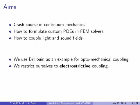
Crash course in continuum mechanics
How to formulate custom PDEs in FEM solvers
How to couple light and sound fields
We use Brillouin as an example for opto-mechanical coupling.
We restrict ourselves to electrostrictive coupling.
Non-Brillouin and non-electrostrictive problems (e. g. cavityopto-mechanics or MEMS) require fundamentally similarmethods.
C. Wolff & M. J. A. Smith Workshop: Opto-acoustic with COMSOL July 15, 2016 3 / 21
Aims
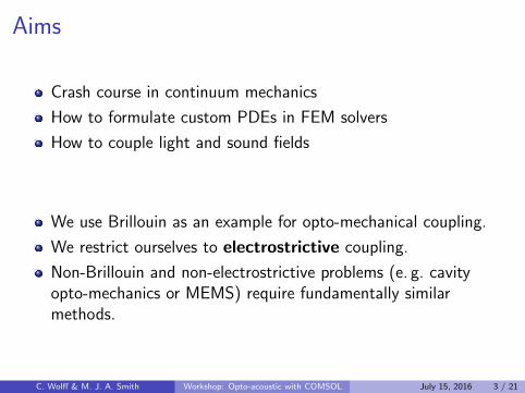
Crash course in continuum mechanics
How to formulate custom PDEs in FEM solvers
How to couple light and sound fields
We use Brillouin as an example for opto-mechanical coupling.
We restrict ourselves to electrostrictive coupling.
Non-Brillouin and non-electrostrictive problems (e. g. cavityopto-mechanics or MEMS) require fundamentally similarmethods.
C. Wolff & M. J. A. Smith Workshop: Opto-acoustic with COMSOL July 15, 2016 3 / 21
Aims
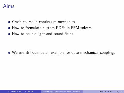
Crash course in continuum mechanics
How to formulate custom PDEs in FEM solvers
How to couple light and sound fields
We use Brillouin as an example for opto-mechanical coupling.
We restrict ourselves to electrostrictive coupling.
Non-Brillouin and non-electrostrictive problems (e. g. cavityopto-mechanics or MEMS) require fundamentally similarmethods.
C. Wolff & M. J. A. Smith Workshop: Opto-acoustic with COMSOL July 15, 2016 3 / 21

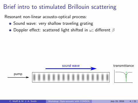
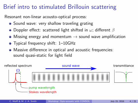
Brief intro to stimulated Brillouin scattering
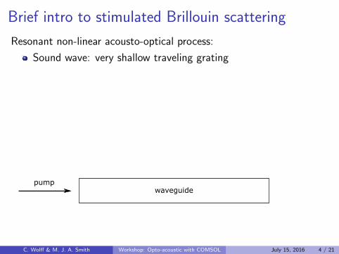
Resonant non-linear acousto-optical process:
Sound wave: very shallow traveling grating
Doppler effect: scattered light shifted in ω; different β
Missing energy and momentum → sound wave amplification
Typical frequency shift: 1–10GHz
Massive difference in optical and acoustic frequencies:sound quasi-static for light field
C. Wolff & M. J. A. Smith Workshop: Opto-acoustic with COMSOL July 15, 2016 4 / 21

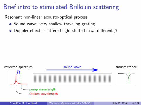
Brief intro to stimulated Brillouin scattering
Resonant non-linear acousto-optical process:
Sound wave: very shallow traveling grating
Doppler effect: scattered light shifted in ω; different β
Missing energy and momentum → sound wave amplification
Typical frequency shift: 1–10GHz
Massive difference in optical and acoustic frequencies:sound quasi-static for light field
pumpwaveguide
C. Wolff & M. J. A. Smith Workshop: Opto-acoustic with COMSOL July 15, 2016 4 / 21
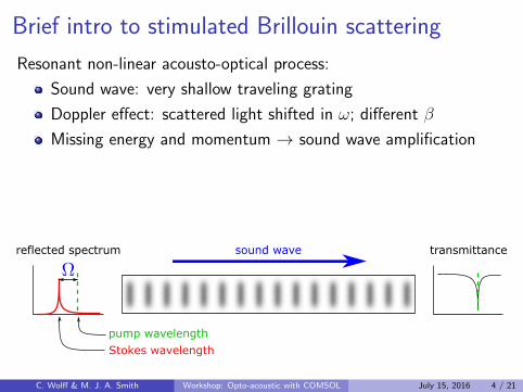
Brief intro to stimulated Brillouin scattering
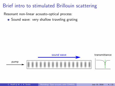
Resonant non-linear acousto-optical process:
Sound wave: very shallow traveling grating
Doppler effect: scattered light shifted in ω; different β
Missing energy and momentum → sound wave amplification
Typical frequency shift: 1–10GHz
Massive difference in optical and acoustic frequencies:sound quasi-static for light field
pumpwaveguide
C. Wolff & M. J. A. Smith Workshop: Opto-acoustic with COMSOL July 15, 2016 4 / 21
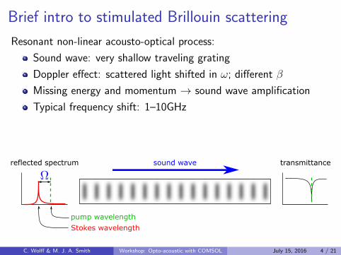
Brief intro to stimulated Brillouin scattering
Resonant non-linear acousto-optical process:
Sound wave: very shallow traveling grating
Doppler effect: scattered light shifted in ω; different β
Missing energy and momentum → sound wave amplification
Typical frequency shift: 1–10GHz
Massive difference in optical and acoustic frequencies:sound quasi-static for light field
sound wave transmittance
pump
C. Wolff & M. J. A. Smith Workshop: Opto-acoustic with COMSOL July 15, 2016 4 / 21
Brief intro to stimulated Brillouin scattering
Resonant non-linear acousto-optical process:
Sound wave: very shallow traveling grating
Doppler effect: scattered light shifted in ω; different β
Missing energy and momentum → sound wave amplification
Typical frequency shift: 1–10GHz
Massive difference in optical and acoustic frequencies:sound quasi-static for light field
sound wave
pump wavelength
Stokes wavelength
transmittancereflected spectrum
C. Wolff & M. J. A. Smith Workshop: Opto-acoustic with COMSOL July 15, 2016 4 / 21
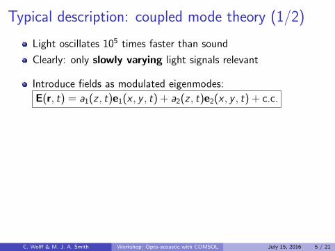
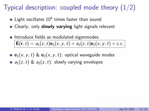
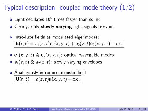
Typical description: coupled mode theory (1/2)
Light oscillates 105 times faster than sound
Clearly: only slowly varying light signals relevant
Introduce fields as modulated eigenmodes:
E(r, t) = a1(z , t)e1(x , y , t) + a2(z , t)e2(x , y , t) + c.c.
e1(x , y , t) & e2(x , y , t): optical waveguide modes
a1(z , t) & a2(z , t): slowly varying envelopes
Analogously introduce acoustic field
U(r, t) = b(z , t)u(x , y , t) + c.c.
u(x , y , t): mechanical displacement field (explained in part 2).
b(z , t): acoustic envelope.
C. Wolff & M. J. A. Smith Workshop: Opto-acoustic with COMSOL July 15, 2016 5 / 21
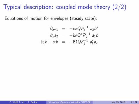
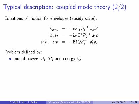
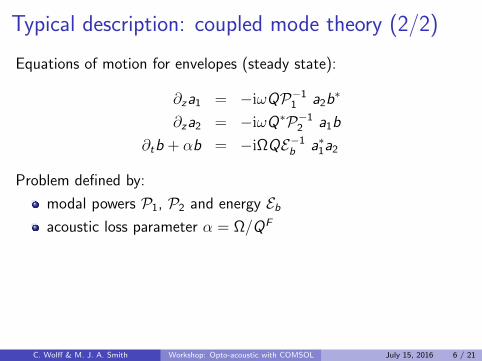
Typical description: coupled mode theory (2/2)
Equations of motion for envelopes (steady state):
∂za1 = −iωQP−11 a2b
∗
∂za2 = −iωQ∗P−12 a1b
∂tb + αb = −iΩQE−1b a∗1a2
Problem defined by:
modal powers P1, P2 and energy Ebacoustic loss parameter α = Ω/QF
opto-acoustic coupling coefficient Q
Experimentally most relevant:
SBS power gain Γ = 2ω|Q|2QF/(P1P2Eb)
C. Wolff & M. J. A. Smith Workshop: Opto-acoustic with COMSOL July 15, 2016 6 / 21
Typical description: coupled mode theory (2/2)
Equations of motion for envelopes (steady state):
∂za1 = −iωQP−11 a2b
∗
∂za2 = −iωQ∗P−12 a1b
∂tb + αb = −iΩQE−1b a∗1a2
Problem defined by:
modal powers P1, P2 and energy Eb
acoustic loss parameter α = Ω/QF
opto-acoustic coupling coefficient Q
Experimentally most relevant:
SBS power gain Γ = 2ω|Q|2QF/(P1P2Eb)
C. Wolff & M. J. A. Smith Workshop: Opto-acoustic with COMSOL July 15, 2016 6 / 21
Typical description: coupled mode theory (2/2)
Equations of motion for envelopes (steady state):
∂za1 = −iωQP−11 a2b
∗
∂za2 = −iωQ∗P−12 a1b
∂tb + αb = −iΩQE−1b a∗1a2
Problem defined by:
modal powers P1, P2 and energy Ebacoustic loss parameter α = Ω/QF
opto-acoustic coupling coefficient Q
Experimentally most relevant:
SBS power gain Γ = 2ω|Q|2QF/(P1P2Eb)
C. Wolff & M. J. A. Smith Workshop: Opto-acoustic with COMSOL July 15, 2016 6 / 21
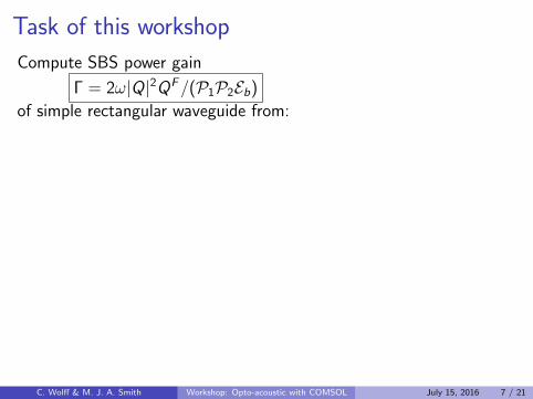
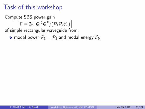
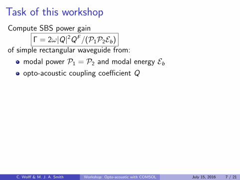
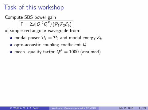
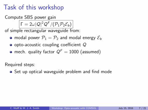
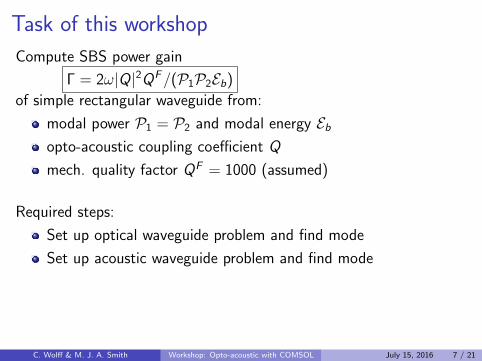
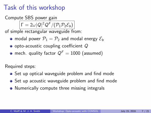
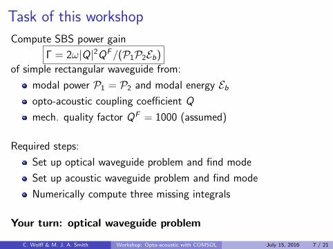
Task of this workshop
Compute SBS power gain
Γ = 2ω|Q|2QF/(P1P2Eb)
of simple rectangular waveguide from:
modal power P1 = P2 and modal energy Ebopto-acoustic coupling coefficient Q
mech. quality factor QF = 1000 (assumed)
Required steps:
Set up optical waveguide problem and find mode
Set up acoustic waveguide problem and find mode
Numerically compute three missing integrals
Your turn: optical waveguide problem
C. Wolff & M. J. A. Smith Workshop: Opto-acoustic with COMSOL July 15, 2016 7 / 21
Task of this workshop
Compute SBS power gain
Γ = 2ω|Q|2QF/(P1P2Eb)
of simple rectangular waveguide from:
modal power P1 = P2 and modal energy Eb
opto-acoustic coupling coefficient Q
mech. quality factor QF = 1000 (assumed)
Required steps:
Set up optical waveguide problem and find mode
Set up acoustic waveguide problem and find mode
Numerically compute three missing integrals
Your turn: optical waveguide problem
C. Wolff & M. J. A. Smith Workshop: Opto-acoustic with COMSOL July 15, 2016 7 / 21
Task of this workshop
Compute SBS power gain
Γ = 2ω|Q|2QF/(P1P2Eb)
of simple rectangular waveguide from:
modal power P1 = P2 and modal energy Ebopto-acoustic coupling coefficient Q
mech. quality factor QF = 1000 (assumed)
Required steps:
Set up optical waveguide problem and find mode
Set up acoustic waveguide problem and find mode
Numerically compute three missing integrals
Your turn: optical waveguide problem
C. Wolff & M. J. A. Smith Workshop: Opto-acoustic with COMSOL July 15, 2016 7 / 21
Task of this workshop
Compute SBS power gain
Γ = 2ω|Q|2QF/(P1P2Eb)
of simple rectangular waveguide from:
modal power P1 = P2 and modal energy Ebopto-acoustic coupling coefficient Q
mech. quality factor QF = 1000 (assumed)
Required steps:
Set up optical waveguide problem and find mode
Set up acoustic waveguide problem and find mode
Numerically compute three missing integrals
Your turn: optical waveguide problem
C. Wolff & M. J. A. Smith Workshop: Opto-acoustic with COMSOL July 15, 2016 7 / 21
Acoustic waveguide problem
C. Wolff & M. J. A. Smith Workshop: Opto-acoustic with COMSOL July 15, 2016 8 / 21

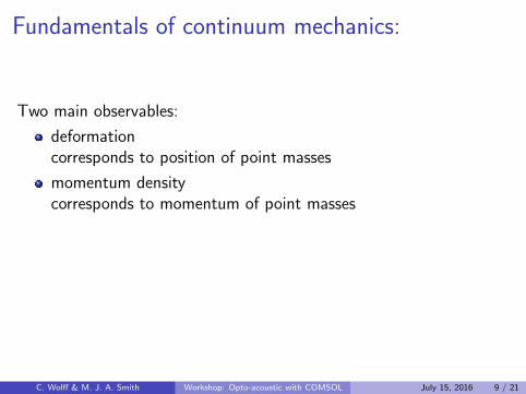
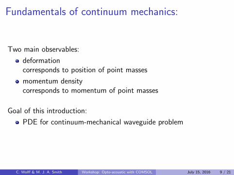
Fundamentals of continuum mechanics:
Two main observables:
deformationcorresponds to position of point masses
momentum densitycorresponds to momentum of point masses
Goal of this introduction:
PDE for continuum-mechanical waveguide problem
C. Wolff & M. J. A. Smith Workshop: Opto-acoustic with COMSOL July 15, 2016 9 / 21
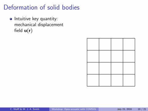
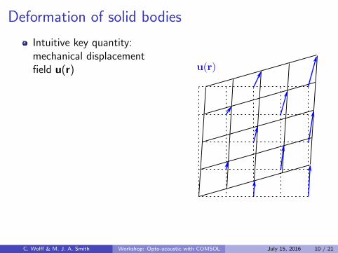
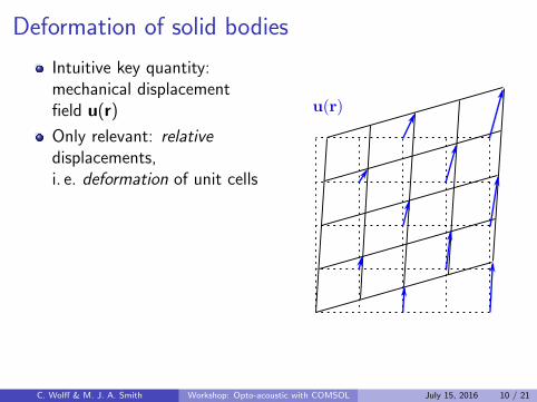
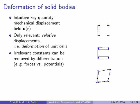
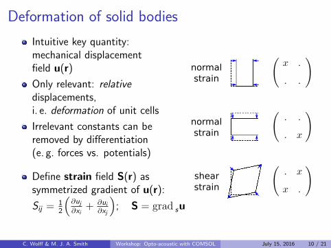
Deformation of solid bodies
Intuitive key quantity:mechanical displacementfield u(r)
Only relevant: relativedisplacements,i. e. deformation of unit cells
Irrelevant constants can beremoved by differentiation(e. g. forces vs. potentials)
Define strain field S(r) assymmetrized gradient of u(r):
Sij = 12
(∂uj∂xi
+ ∂ui∂xj
); S = grad su
C. Wolff & M. J. A. Smith Workshop: Opto-acoustic with COMSOL July 15, 2016 10 / 21
Deformation of solid bodies
Intuitive key quantity:mechanical displacementfield u(r)
Only relevant: relativedisplacements,i. e. deformation of unit cells
Irrelevant constants can beremoved by differentiation(e. g. forces vs. potentials)
Define strain field S(r) assymmetrized gradient of u(r):
Sij = 12
(∂uj∂xi
+ ∂ui∂xj
); S = grad su
normal strain
normal strain
shear strain
C. Wolff & M. J. A. Smith Workshop: Opto-acoustic with COMSOL July 15, 2016 10 / 21
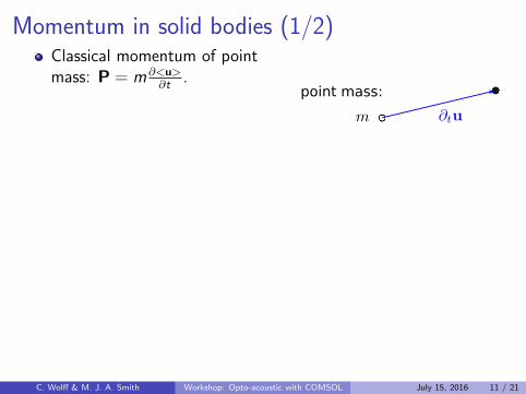
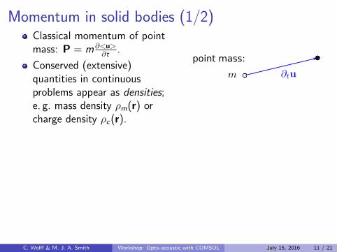
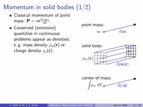
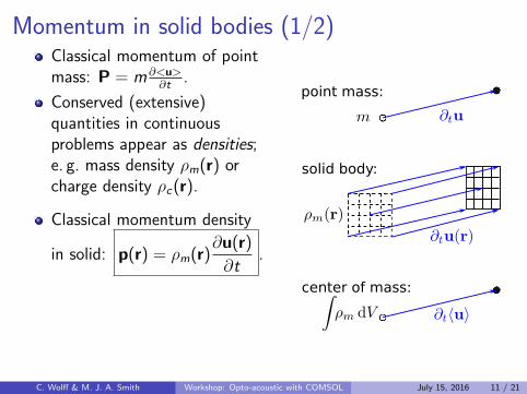
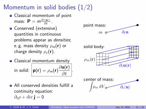
Momentum in solid bodies (1/2)Classical momentum of pointmass: P = m ∂<u>
∂t.
Conserved (extensive)quantities in continuousproblems appear as densities;e. g. mass density ρm(r) orcharge density ρc(r).
Classical momentum density
in solid: p(r) = ρm(r)∂u(r)
∂t.
All conserved densities fulfill acontinuity equation:∂tρ + div j = 0
point mass:
C. Wolff & M. J. A. Smith Workshop: Opto-acoustic with COMSOL July 15, 2016 11 / 21
Momentum in solid bodies (1/2)Classical momentum of pointmass: P = m ∂<u>
∂t.
Conserved (extensive)quantities in continuousproblems appear as densities;e. g. mass density ρm(r) orcharge density ρc(r).
Classical momentum density
in solid: p(r) = ρm(r)∂u(r)
∂t.
All conserved densities fulfill acontinuity equation:∂tρ + div j = 0
point mass:
center of mass:
solid body:
C. Wolff & M. J. A. Smith Workshop: Opto-acoustic with COMSOL July 15, 2016 11 / 21
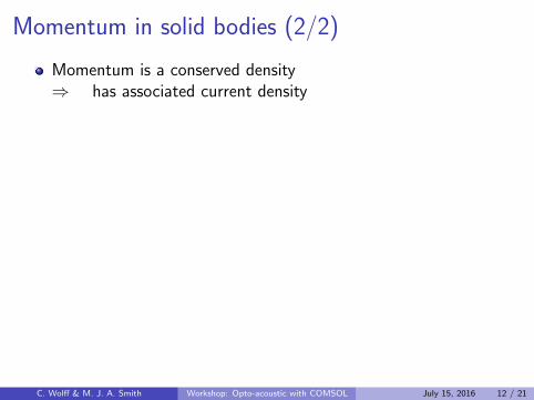
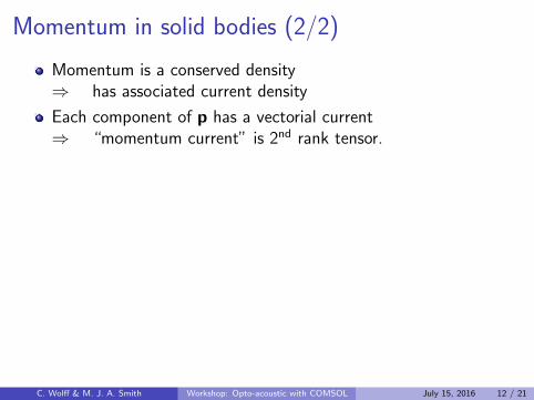
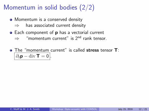
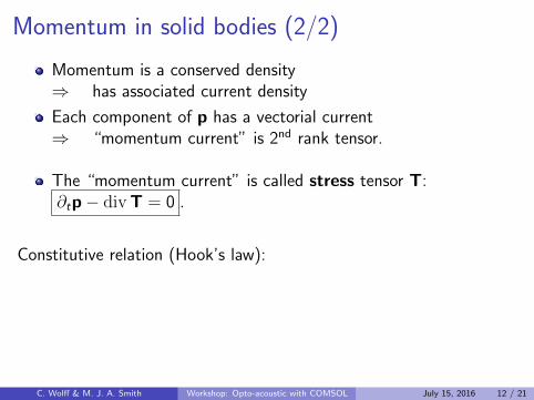
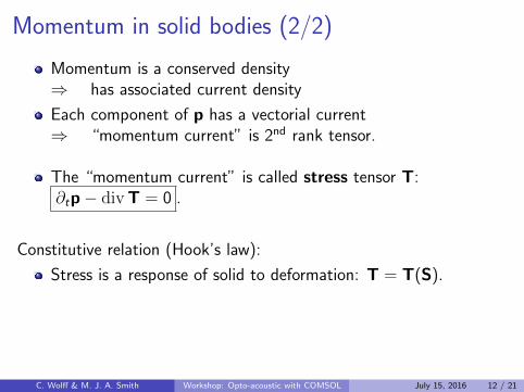
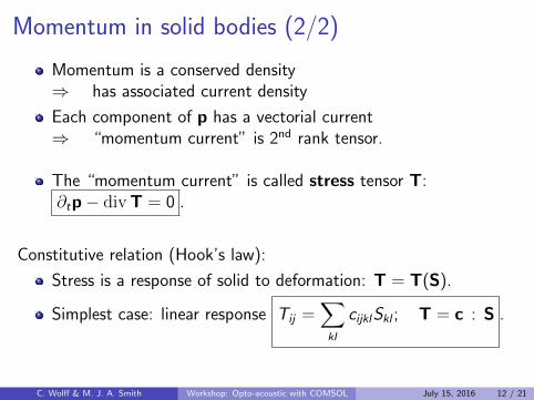
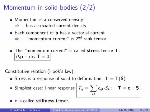
Momentum in solid bodies (2/2)
Momentum is a conserved density⇒ has associated current density
Each component of p has a vectorial current⇒ “momentum current” is 2nd rank tensor.
The “momentum current” is called stress tensor T:∂tp− divT = 0 .
Constitutive relation (Hook’s law):
Stress is a response of solid to deformation: T = T(S).
Simplest case: linear response Tij =∑kl
cijklSkl ; T = c : S .
c is called stiffness tensor.
C. Wolff & M. J. A. Smith Workshop: Opto-acoustic with COMSOL July 15, 2016 12 / 21

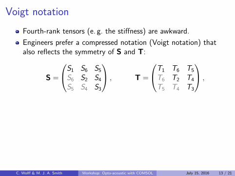
Voigt notation
Fourth-rank tensors (e. g. the stiffness) are awkward.
Engineers prefer a compressed notation (Voigt notation) thatalso reflects the symmetry of S and T:
S =
S1 S6 S5
S6 S2 S4
S5 S4 S3
, T =
T1 T6 T5
T6 T2 T4
T5 T4 T3
,
S and T can be organized as “vectors” with 6 entries
This allows to represent c as a 6× 6-matrix
For isotropic materials c has only two free parameters, e. g.Youngs modulus E andPoisson number νand c contains many zeros.
C. Wolff & M. J. A. Smith Workshop: Opto-acoustic with COMSOL July 15, 2016 13 / 21
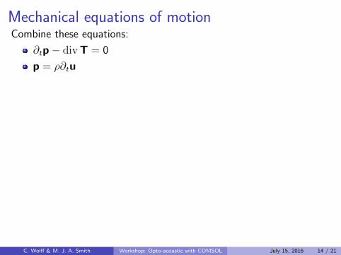
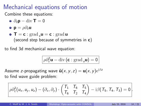
Mechanical equations of motionCombine these equations:
∂tp− divT = 0
p = ρ∂tu
T = c : grad su = c : gradu(second step because of symmetries in c)
to find 3d mechanical wave equation:
ρ∂2t u− div (c : grad su) = 0
Assume z-propagating wave u(x , y , z) = u(x , y)eiβz
to find wave guide problem:
ρ∂2t (ux , uy , uz)− (∂x , ∂y ) ·
(T1 T6 T5
T6 T2 T4
)− iβ(T5,T4,T3) = 0 .
C. Wolff & M. J. A. Smith Workshop: Opto-acoustic with COMSOL July 15, 2016 14 / 21
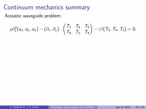
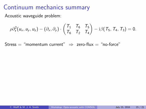
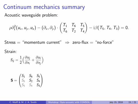
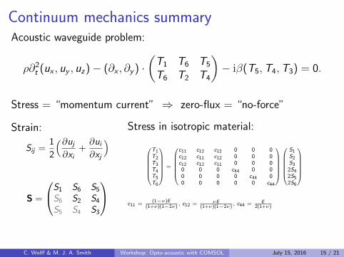
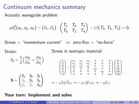
Continuum mechanics summaryAcoustic waveguide problem:
ρ∂2t (ux , uy , uz)− (∂x , ∂y ) ·
(T1 T6 T5
T6 T2 T4
)− iβ(T5,T4,T3) = 0.
Stress = “momentum current” ⇒ zero-flux = “no-force”
Strain: Stress in isotropic material:
Sij =1
2
(∂uj∂xi
+∂ui∂xj
)
S =
S1 S6 S5
S6 S2 S4
S5 S4 S3
T1T2T3T4T5T6
=
c11 c12 c12 0 0 0c12 c11 c12 0 0 0c12 c12 c11 0 0 00 0 0 c44 0 00 0 0 0 c44 00 0 0 0 0 c44
S1S2S3
2S42S52S6
c11 =(1−ν)E
(1+ν)(1−2ν), c12 = νE
(1+ν)(1−2ν), c44 = E
2(1+ν)
Your turn: Implement and solve
C. Wolff & M. J. A. Smith Workshop: Opto-acoustic with COMSOL July 15, 2016 15 / 21
Continuum mechanics summaryAcoustic waveguide problem:
ρ∂2t (ux , uy , uz)− (∂x , ∂y ) ·
(T1 T6 T5
T6 T2 T4
)− iβ(T5,T4,T3) = 0.
Stress = “momentum current” ⇒ zero-flux = “no-force”
Strain:
Stress in isotropic material:
Sij =1
2
(∂uj∂xi
+∂ui∂xj
)
S =
S1 S6 S5
S6 S2 S4
S5 S4 S3
T1T2T3T4T5T6
=
c11 c12 c12 0 0 0c12 c11 c12 0 0 0c12 c12 c11 0 0 00 0 0 c44 0 00 0 0 0 c44 00 0 0 0 0 c44
S1S2S3
2S42S52S6
c11 =(1−ν)E
(1+ν)(1−2ν), c12 = νE
(1+ν)(1−2ν), c44 = E
2(1+ν)
Your turn: Implement and solve
C. Wolff & M. J. A. Smith Workshop: Opto-acoustic with COMSOL July 15, 2016 15 / 21
Continuum mechanics summaryAcoustic waveguide problem:
ρ∂2t (ux , uy , uz)− (∂x , ∂y ) ·
(T1 T6 T5
T6 T2 T4
)− iβ(T5,T4,T3) = 0.
Stress = “momentum current” ⇒ zero-flux = “no-force”
Strain: Stress in isotropic material:
Sij =1
2
(∂uj∂xi
+∂ui∂xj
)
S =
S1 S6 S5
S6 S2 S4
S5 S4 S3
T1T2T3T4T5T6
=
c11 c12 c12 0 0 0c12 c11 c12 0 0 0c12 c12 c11 0 0 00 0 0 c44 0 00 0 0 0 c44 00 0 0 0 0 c44
S1S2S3
2S42S52S6
c11 =(1−ν)E
(1+ν)(1−2ν), c12 = νE
(1+ν)(1−2ν), c44 = E
2(1+ν)
Your turn: Implement and solve
C. Wolff & M. J. A. Smith Workshop: Opto-acoustic with COMSOL July 15, 2016 15 / 21
Continuum mechanics summaryAcoustic waveguide problem:
ρ∂2t (ux , uy , uz)− (∂x , ∂y ) ·
(T1 T6 T5
T6 T2 T4
)− iβ(T5,T4,T3) = 0.
Stress = “momentum current” ⇒ zero-flux = “no-force”
Strain: Stress in isotropic material:
Sij =1
2
(∂uj∂xi
+∂ui∂xj
)
S =
S1 S6 S5
S6 S2 S4
S5 S4 S3
T1T2T3T4T5T6
=
c11 c12 c12 0 0 0c12 c11 c12 0 0 0c12 c12 c11 0 0 00 0 0 c44 0 00 0 0 0 c44 00 0 0 0 0 c44
S1S2S3
2S42S52S6
c11 =(1−ν)E
(1+ν)(1−2ν), c12 = νE
(1+ν)(1−2ν), c44 = E
2(1+ν)
Your turn: Implement and solve
C. Wolff & M. J. A. Smith Workshop: Opto-acoustic with COMSOL July 15, 2016 15 / 21
Calculation of an electrostrictive SBS gain
C. Wolff & M. J. A. Smith Workshop: Opto-acoustic with COMSOL July 15, 2016 16 / 21
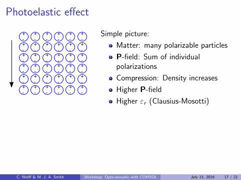
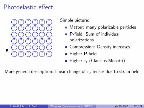
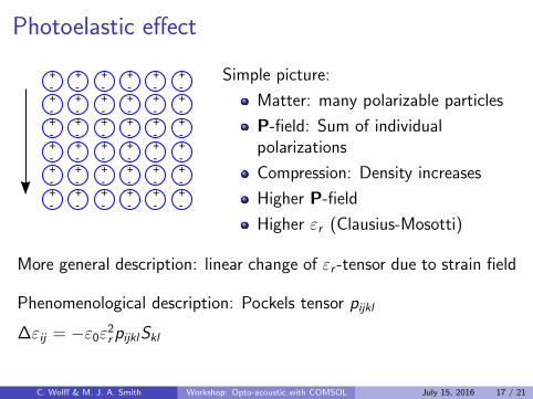
Photoelastic effect
+
-
+
-
+
-
+
-
+
-
+
-
+
-
+
-
+
-
+
-
+
-
+
-
+
-
+
-
+
-
+
-
+
-
+
-
+
-
+
-
+
-
+
-
+
-
+
-
+
-
+
-
+
-
+
-
+
-
+
-
+
-
+
-
+
-
+
-
+
-
+
-
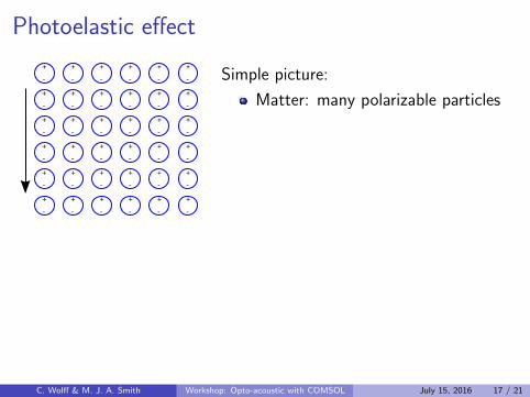
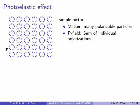
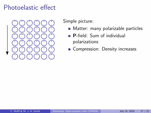
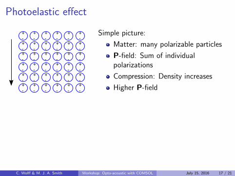
Simple picture:
Matter: many polarizable particles
P-field: Sum of individualpolarizations
Compression: Density increases
Higher P-field
Higher εr (Clausius-Mosotti)
More general description: linear change of εr -tensor due to strain field
Phenomenological description: Pockels tensor pijkl
∆εij = −ε0ε2r pijklSkl
C. Wolff & M. J. A. Smith Workshop: Opto-acoustic with COMSOL July 15, 2016 17 / 21
Photoelastic effect
+
-
+
-
+
-
+
-
+
-
+
-
+
-
+
-
+
-
+
-
+
-
+
-
+
-
+
-
+
-
+
-
+
-
+
-
+
-
+
-
+
-
+
-
+
-
+
-
+
-
+
-
+
-
+
-
+
-
+
-
+
-
+
-
+
-
+
-
+
-
+
-
Simple picture:
Matter: many polarizable particles
P-field: Sum of individualpolarizations
Compression: Density increases
Higher P-field
Higher εr (Clausius-Mosotti)
More general description: linear change of εr -tensor due to strain field
Phenomenological description: Pockels tensor pijkl
∆εij = −ε0ε2r pijklSkl
C. Wolff & M. J. A. Smith Workshop: Opto-acoustic with COMSOL July 15, 2016 17 / 21
Photoelastic effect
+-
+-
+-
+-
+-
+-
+-
+-
+-
+-
+-
+-
+-
+-
+-
+-
+-
+-
+-
+-
+-
+-
+-
+-
+-
+-
+-
+-
+-
+-
+-
+-
+-
+-
+-
+-
Simple picture:
Matter: many polarizable particles
P-field: Sum of individualpolarizations
Compression: Density increases
Higher P-field
Higher εr (Clausius-Mosotti)
More general description: linear change of εr -tensor due to strain field
Phenomenological description: Pockels tensor pijkl
∆εij = −ε0ε2r pijklSkl
C. Wolff & M. J. A. Smith Workshop: Opto-acoustic with COMSOL July 15, 2016 17 / 21
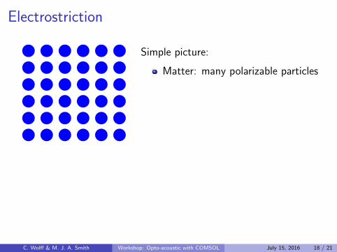
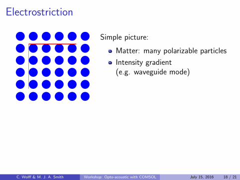
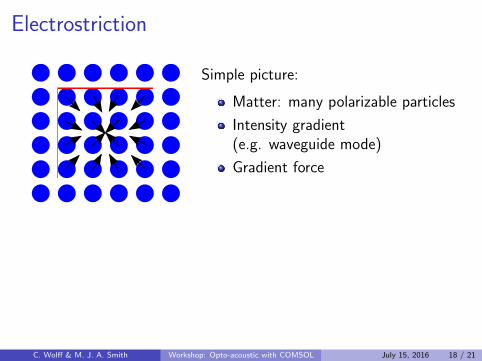
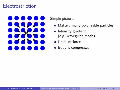
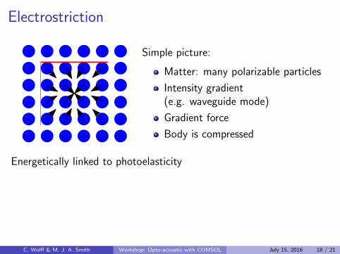
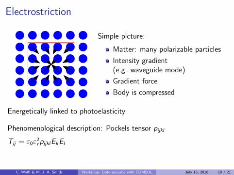
Electrostriction
Simple picture:
Matter: many polarizable particles
Intensity gradient(e.g. waveguide mode)
Gradient force
Body is compressed
Energetically linked to photoelasticity
Phenomenological description: Pockels tensor pijkl
Tij = ε0ε2r pijklEkEl
C. Wolff & M. J. A. Smith Workshop: Opto-acoustic with COMSOL July 15, 2016 18 / 21
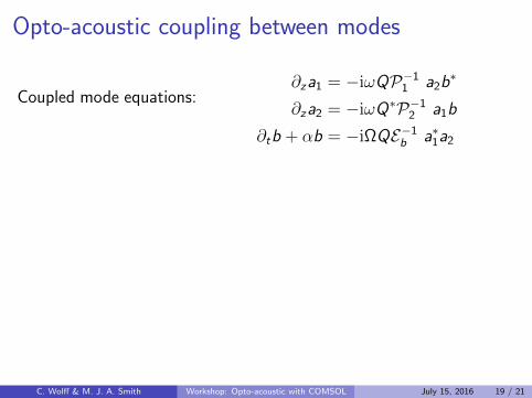
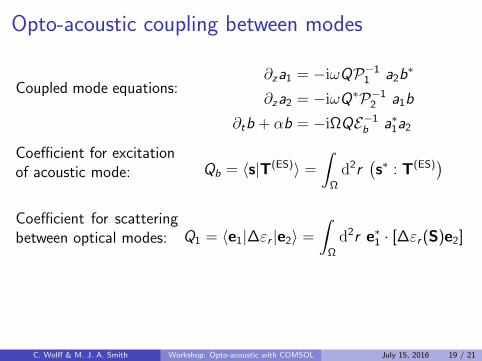
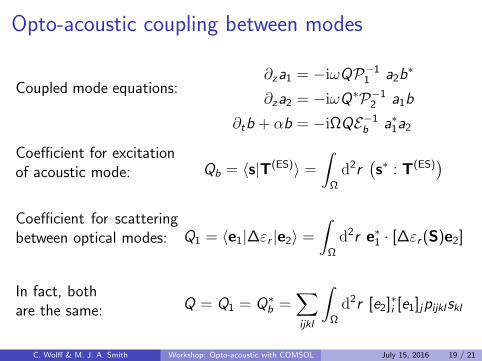
Opto-acoustic coupling between modes
Coupled mode equations:∂za1 = −iωQP−1
1 a2b∗
∂za2 = −iωQ∗P−12 a1b
∂tb + αb = −iΩQE−1b a∗1a2
Coefficient for excitationof acoustic mode: Qb = 〈s|T(ES)〉 =
∫Ω
d2r(s∗ : T(ES)
)Coefficient for scatteringbetween optical modes: Q1 = 〈e1|∆εr |e2〉 =
∫Ω
d2r e∗1 · [∆εr (S)e2]
In fact, bothare the same: Q = Q1 = Q∗
b =∑ijkl
∫Ω
d2r [e2]∗i [e1]jpijklskl
C. Wolff & M. J. A. Smith Workshop: Opto-acoustic with COMSOL July 15, 2016 19 / 21
Opto-acoustic coupling between modes
Coupled mode equations:∂za1 = −iωQP−1
1 a2b∗
∂za2 = −iωQ∗P−12 a1b
∂tb + αb = −iΩQE−1b a∗1a2
Coefficient for excitationof acoustic mode: Qb = 〈s|T(ES)〉 =
∫Ω
d2r(s∗ : T(ES)
)
Coefficient for scatteringbetween optical modes: Q1 = 〈e1|∆εr |e2〉 =
∫Ω
d2r e∗1 · [∆εr (S)e2]
In fact, bothare the same: Q = Q1 = Q∗
b =∑ijkl
∫Ω
d2r [e2]∗i [e1]jpijklskl
C. Wolff & M. J. A. Smith Workshop: Opto-acoustic with COMSOL July 15, 2016 19 / 21
Opto-acoustic coupling between modes
Coupled mode equations:∂za1 = −iωQP−1
1 a2b∗
∂za2 = −iωQ∗P−12 a1b
∂tb + αb = −iΩQE−1b a∗1a2
Coefficient for excitationof acoustic mode: Qb = 〈s|T(ES)〉 =
∫Ω
d2r(s∗ : T(ES)
)Coefficient for scatteringbetween optical modes: Q1 = 〈e1|∆εr |e2〉 =
∫Ω
d2r e∗1 · [∆εr (S)e2]
In fact, bothare the same: Q = Q1 = Q∗
b =∑ijkl
∫Ω
d2r [e2]∗i [e1]jpijklskl
C. Wolff & M. J. A. Smith Workshop: Opto-acoustic with COMSOL July 15, 2016 19 / 21
Opto-acoustic coupling between modes
Coupled mode equations:∂za1 = −iωQP−1
1 a2b∗
∂za2 = −iωQ∗P−12 a1b
∂tb + αb = −iΩQE−1b a∗1a2
Coefficient for excitationof acoustic mode: Qb = 〈s|T(ES)〉 =
∫Ω
d2r(s∗ : T(ES)
)Coefficient for scatteringbetween optical modes: Q1 = 〈e1|∆εr |e2〉 =
∫Ω
d2r e∗1 · [∆εr (S)e2]
In fact, bothare the same: Q = Q1 = Q∗
b =∑ijkl
∫Ω
d2r [e2]∗i [e1]jpijklskl
C. Wolff & M. J. A. Smith Workshop: Opto-acoustic with COMSOL July 15, 2016 19 / 21
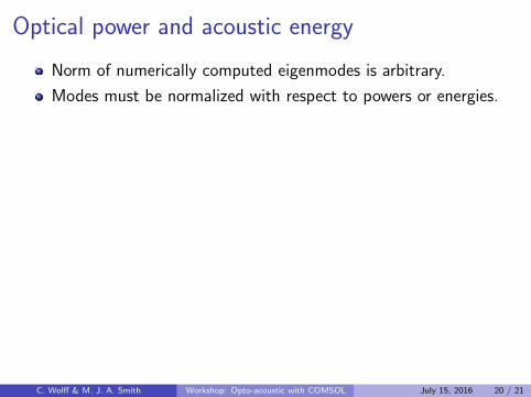
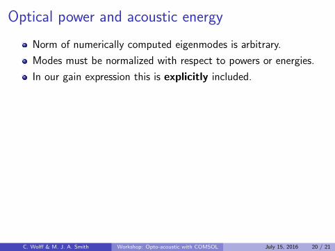
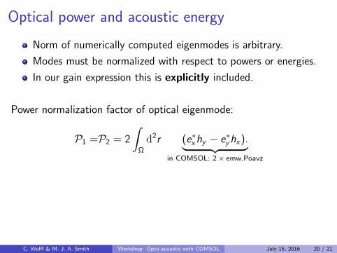
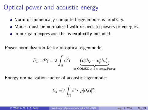
Optical power and acoustic energy
Norm of numerically computed eigenmodes is arbitrary.
Modes must be normalized with respect to powers or energies.
In our gain expression this is explicitly included.
Power normalization factor of optical eigenmode:
P1 =P2 = 2
∫Ω
d2r (e∗xhy − e∗yhx).︸ ︷︷ ︸in COMSOL: 2 × emw.Poavz
Energy normalization factor of acoustic eigenmode:
Eb =2
∫Ω
d2r ρ|∂tu|2.
C. Wolff & M. J. A. Smith Workshop: Opto-acoustic with COMSOL July 15, 2016 20 / 21

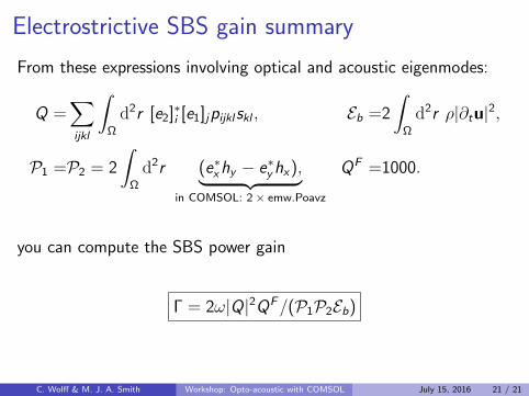
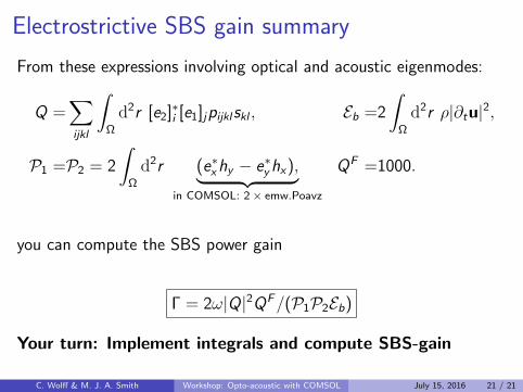
Electrostrictive SBS gain summary
From these expressions involving optical and acoustic eigenmodes:
Q =∑ijkl
∫Ω
d2r [e2]∗i [e1]jpijklskl , Eb =2
∫Ω
d2r ρ|∂tu|2,
P1 =P2 = 2
∫Ω
d2r (e∗xhy − e∗yhx),︸ ︷︷ ︸in COMSOL: 2 × emw.Poavz
QF =1000.
you can compute the SBS power gain
Γ = 2ω|Q|2QF/(P1P2Eb)
Your turn: Implement integrals and compute SBS-gain
C. Wolff & M. J. A. Smith Workshop: Opto-acoustic with COMSOL July 15, 2016 21 / 21