Working Paper Series

WP-18-02

Do School Spending Cuts Matter? Evidence from the Great Recession

C. Kirabo JacksonProfessor of Human Development and Social Policy

IPR FellowNorthwestern University

Cora WiggerGraduate Student

Northwestern University

Heyu XiongGraduate Student

Northwestern University

Version: January 9, 2018

DRAFT Please do not quote or distribute without permission.

2

ABSTRACT

Audits of public school budgets routinely find evidence of waste. Also, recent evidence finds that when school budgets are strained, public schools can employ cost-saving measures with no ill-effect on students. The researchers theorize that if budget cuts induce schools to eliminate wasteful spending, the effects of spending cuts may be small (and even zero). To explore this empirically, they examine how student performance responded to school spending cuts induced by the Great Recession. They link nationally representative test score and survey data to school spending data and isolate variation in recessionary spending cuts that were unrelated to changes in economic conditions. Consistent with the theory, districts that faced large revenue cuts disproportionately reduced spending on non-core operations. However, they still reduced core operational spending to some extent. A 10 percent school spending cut reduced test scores by about 7.8 percent of a standard deviation. Moreover, a 10 percent spending reduction during all four high-school years was associated with 2.6 percentage points lower graduation rates. While the researchers' estimates are smaller than some in the literature, spending cuts do matter.

Do School Spending Cuts Matter? Evidence from theGreat Recession∗

C. Kirabo JacksonNorthwestern University and NBER

Cora WiggerNorthwestern University

Heyu XiongNorthwestern University

January 9, 2018

Abstract

Audits of public school budgets routinely find evidence of waste. Also, recent evidencefinds that when school budgets are strained, public schools can employ cost-saving measureswith no ill-effect on students. We theorize that if budget cuts induce schools to eliminatewasteful spending, the effects of spending cuts may be small (and even zero). To explore thisempirically, we examine how student performance responded to school spending cuts inducedby the Great Recession. We link nationally representative test score and survey data to schoolspending data and isolate variation in recessionary spending cuts that were unrelated to changesin economic conditions. Consistent with the theory, districts that faced large revenue cutsdisproportionately reduced spending on non-core operations. However, they still reduced coreoperational spending to some extent. A 10 percent school spending cut reduced test scores byabout 7.8 percent of a standard deviation. Moreover, a 10 percent spending reduction during allfour high-school years was associated with 2.6 percentage points lower graduation rates. Whileour estimates are smaller than some in the literature, spending cuts do matter.

I IntroductionFor decades researchers have debated whether there is a causal relationship between increased

school spending and students outcomes (Coleman, 1990). Until recently, much of the evidence onthis had been correlational and suggested little association between school spending and student

∗Jackson: Northwestern University, 2120 Campus Drive, Evanston IL 60208 (email:kirabo-jackson@northwestern.edu). Wigger: Northwestern University, 2120 Campus Drive, Evanston IL 60208(email:CoraWigger2021@u.northwestern.edu). Xiong: Northwestern University, 2211 Campus Dr,(email:HeyuXiong2018@u.northwestern.edu). The statements made and views expressed are solely the respon-sibility of the authors. Wigger and Xiong are grateful for financial support from the US Department of Education,Institute of Education Sciences through its Multidisciplinary Program in Education Sciences (Grant Award #R305B140042).

outcomes (Hanushek 1997; Betts 1996). However, several well-identified studies now find thatlarge permanent increases in school spending due to the passage of school finance reforms improvedstudent longer run outcomes such as adult wages (Jackson et al., 2016) and crime (Johnson andJackson, 2017), medium-run outcomes such as high school completion (Candelaria and Shores,2017), and short run outcomes such as SAT scores (Card and Payne, 2002) and standardized testscores (Lafortune et al., 2018). This collection of studies is now being used both to to advocate forincreased school spending, and also oppose reductions in schools budgets (Barnum, 2016).

However, audits of public school budgets routinely find evidence of waste and bloat (Ross2015). This suggests that in the face of public school budget cuts, one could reduce school spend-ing with little to no deleterious effects on children. The basic logic is that while schools mayengage in wasteful spending when budgets are growing (e.g. Liebman and Mahoney 2017), hardfinancial times create incentives that induce firms and workers to curb wasteful spending and “make

do with less” (Lazear et al. 2016). There is empirical support for this idea; in the wake of recession-ary budget cuts, many districts induced expensive experienced teachers to retire early (Fitzpatrickand Lovenheim 2014), others deferred scheduled maintenance and eliminated non-essential travel(Ellerson 2010), and some districts operated schools for only four days per week (Anderson andWalker 2015).1 Remarkably, both Fitzpatrick and Lovenheim (2014) and Anderson and Walker(2015) find that these cost-saving measures improve student outcomes; evidence that public schoolsmay not always allocate their budgets in a manner that maximizes student achievement.

The increased use of cost-saving practices during recessions creates a puzzle. If such measuresreduce costs with no ill-effects for students, why don’t schools use them all the time? To rationalizethese patterns, we theorize that if (a) there is waste and bloat in the system, and (b) schools arepunished for poor outcomes more than they are rewarded for good outcomes, schools will be morelikely to cut back on wasteful spending practices during recessions. A direct implication of thismodel is that even if spending increases lead to improved outcomes, spending reductions may havelittle or no deleterious effects. To test this notion empirically, we examine the causal effect ofreductions in school spending due to budgetary cuts in response to the Great Recession.

Our main outcome of interest is student test scores from the restricted individual-level Na-tional Assessment of Educational Progress (NAEP) data. The NAEP, commonly referred to as “theNation’s Report Card,” tests state-representative samples of over one hundred thousand studentsin math and reading in 4th and 8th grade every two years. We focus on exams given between2002 and 2015. We link these test score data to district level-spending data from the CommonCore of Data (CCD) between 2000 and 2015. To examine longer-run outcomes we also employthe Integrated Public Use Microdata Series (IPUMS) which contains information on high schoolcompletion among a representative sample of individuals in a state.

1As of 2016, this has been tried in over 100 districts across several U.S. states (Hill and Heyward, 2017).

2

To isolate plausibly exogenous variation in school spending, our identification strategy exploitsthe fact that states that funded high shares of their pre-recession school budgets from state sourceswere those that saw the largest reductions in per pupil spending in the wake of the Great Recession.That is, because state tax collections fell dramatically during the recession, states that were histor-ically most reliant on state tax collections to fund public schools saw the deepest school spendingcuts (Evans et al. 2017; Shores and Steinberg 2017). Our instrument is, therefore, the interactionbetween the share of state K12 spending that came from state sources in 2008 and the numberof years post-recession. Our empirical strategy relies on the assumption that states with differentlevels of reliance on state revenue sources were not differentially affected by the recession for rea-sons other than through school spending. We present much evidence that our instrument is bothrelevant and likely exogenous. Specifically, we demonstrate that (a) both test scores and economicconditions in districts with high shares of state spending from state sources were on similar pre-recession trajectories as those with low shares, (b) high shares of state spending from state sourcesis a very strong predictor of reductions in school spending only after the recession, (c) changesin school spending as predicted by the instrument are unrelated to changes in unemployment orchild poverty, and (d) adding controls for economic conditions at both the state and local levels hasvirtually no effect on our estimated relationships between school spending and student outcomes.

Using our instrumental variables strategy, we find that districts responded to spending cuts bydisproportionately cutting more from construction expenditures and less from core K12 spending.While construction spending makes up only 5 percent of the average schools budget, it accountedfor 47 percent of the reduced spending. Conversely, while current K12 operating spending accountsfor 86 percent of all spending it accounted for only 55 percent of spending reductions. Thesepatterns stand in contrast to those documented for spending increases due to school finance reforms(Jackson et al., 2016) and suggest that the marginal propensity to spend on different inputs varieswhen there are spending increases than when there are spending reductions. This is consistent withour model in which districts become more efficient at spending when times are hard. The resultsalso suggest that the budget cuts were sufficiently large that, even if there were some bloat, districtswere forced to make cuts that likely hindered student outcomes.

Looking at test scores, on average, a 10 percent reduction in per-pupil spending led to about0.078 standard deviations lower test scores (p-value<0.01). Reassuringly, these effects are un-changed as one controls for the prevailing economic conditions; suggesting that our effects on testscores are driven by the changes in public school spending only. We test this further, by show-ing that while recessionary school spending cuts are strongly associated with reductions in public

school test scores, they are not systematically related to changes in private school test scores. Wealso examine effects by grade level and subject. As is common in other settings, effects are largerfor math than reading. A 10 percent reduction in per-pupil spending leads to roughly 3.55 percent

3

of a standard deviation lower scores in reading and 11.83 percent of a standard deviation lowerscores in math. These estimated effects are about half as large as Lafortune et al. (2018). 2 To putthese effects into perspective, these effect sizes are roughly equivalent to that of reducing teacherquality by one standard deviation (i.e. having all teachers in the district go from average quality tothe 15th percentile) (Jackson et al., 2014).

To examine effects on longer-run outcomes, we test for whether exposure to recessionary spend-ing cuts had deleterious effects on high school completion using Census data. Within a differencein differences framework (comparing the difference in outcomes between exposed and unexposedcohorts in states that had smaller or larger recessionary budgets cuts), exposure to the larger reces-sionary school spending cuts reduced high school completion for those who were exposed duringtheir elementary school years. More specifically, a 10 percent reduction in per pupil spendingacross all four of an individual’s high-school-age years reduced the likelihood of completing highschool by 2.7 percentage points. This is similar to estimates based on school finance reforms inrecent years (e.g. Jackson et al. (2016) and Candelaria and Shores (2017)).

Overall, our theoretical framework and our analysis of school budgets suggest that the effectof spending cuts may be smaller than those of spending increases. At the same time, our analysisof student outcomes are inconsistent with spending cuts having no deleterious effect on studentoutcomes at all. Our findings contribute to the long-standing debate around whether school spend-ing matters by showing that (a) spending cuts harm students, and (b) spending matters even whenusing variation other than that due to school finance reforms. A distinguishing feature of this workis that our results shed light on how school districts may react asymmetrically to increases versusdecreases in budgets. Accordingly, these results contribute to the field of behavioral public finance.Finally, our results deepen understanding of the long-run effects of growing up during a recession.While it is well-documented that growing up during a recession can lead to long lasting ill-effectsthrough channels such as parental job displacement (Oreopoulos et al. 2008; Ananat et al. 2011;Stevens and Schaller 2011) and increased food insecurity (Gundersen et al. 2011; Schanzenbachand Lauren 2017), we provide the first evidence that recessions have lasting ill-effects on youngindividuals through their effects on the governments’ abilities to provide public education services.

The remainder of the paper is as follows. Section II present a theoretical framework withinwhich the effects of spending reductions may differ from those of spending increases. Section IIIdescribes the data. Section IV describes the empirical strategy. Section V presents the main re-sults, Section V.1 explores mechanisms, and Section V.2.2 presents robustness checks. Section VIpresents some discussion of the findings and concludes.

2Lafortune et al. (2018) find that “The implied impact is between 0.12 and 0.24 standard deviations per $1,000 perpupil in annual spending.” We take the midpoint of these values 0.18 as there overall estimate. Average spending levelsin our period were $9540.35, so that a $1,000 is roughly a 10 percent increase.

4

II Theoretical FrameworkWe present a theoretical framework for thinking about why the marginal effect of spending in-

creases could be large and positive, while those for spending reductions could be much smaller andpossibly zero. Our framework highlights that for asymmetric spending effects to emerge requiresgreater incentives to reduce waste when budgets contract than when they are growing. Informed bythe idea that voters may be loss averse (Kahneman and Tversky, 1979) and may pay more attentionto bad outcomes than good (Lau, 1982), we present a framework with such asymmetric incentives.

In our simple model, a school administrator faces a reward system imposed by parents andchooses how to spend the district budget. The annual budget, B is exogenous. Districts spend τ onthings that are valued by school administrators, but are not productive for students. We refer to thisunproductive spending as “slack”. It may take the form of job perks (such as nice coffee lounges,or non-essential travel) or inefficient spending (e.g. educators hold back on efforts to locate thecheapest textbooks or supplies). With the remaining budget, (B− τ), school districts maximizestudent output. To maximize output, districts spend the first productive dollar on the input with thehighest marginal output per dollar spent, and then spend the next dollar on the the remaining inputwith the highest marginal output per dollar, and keep doing this until the productive budget is spent.Maximum student output (y∗) is therefore a concave increasing function of the productive budgetsuch that y∗ = f (B− τ), where f ′ > 0 and f ′′ ≤ 0.3

School administrators value slack directly g(τ), where g′ > 0, and receive some payoff basedon the student outcomes from parents. Parents may be loss averse (Kahneman and Tversky, 1979)such that they punish test score reductions more harshly than they reward increases. This notionthat public officials are differentially punished for bad outcomes has been documented by politicalscientists (e.g. Lau (1982) and others). For simplicity, we model this as a utility penalty (P) foroutcomes that are worse than in the previous year. Where we index time with the subscript t, theresulting administrator’s utility is as below.

Ut = g(τt)+ f (Bt− τt) i f yt ≥ yt−1

Ut = g(τt)+ f (Bt− τt)−P i f yt < yt−1(1)

The school administrator’s problem is to choose the level of slack τ to maximize their utility giventhe budget they receive and the reward structure imposed by parents.

Case 1: Symmetric rewards (i.e. P=0)

The problem simplifies to the case where the administrator chooses τ to equate the marginalbenefit of one dollar in ”slack” to the marginal payoff from the forgone outcome growth associated

3The assumption that f ′ > 0 is required for the the indirect outcome function to be invertible. This assumption isnot required for the key result that spending increases may have a differently sized effect as spending reductions.

5

with that dollar of slack. That is, dg/dτ =−d f/dτ . So long as τ is a normal good, the optimal slacklevel τ∗ is an increasing function of B. As such, the the utility maximizing level of the outcome y∗

is an increasing function of B. That is, y∗ = f (B− τ∗(B)) = h(B). Under the assumption that y isa normal good d[B− τ∗(B)]/dB > 0, so that h′ > 0, and h(B) is invertible. As such, the increasein equilibrium output y∗ when the budget goes from B to B+ 1 is the same size as the reductionin output when the budget goes from B+ 1 to B. That is, with symmetric rewards, the effect ofspending increases and decreases are opposite in sign and equal in magnitude.

Case 2: Asymmetric rewards due to loss aversion (i.e. P > 0)

From the assumption that both goods (τ and yt) are normal, any spending increase (from B toB+ 1 ) will go toward increasing both test score growth and slack. Accordingly, for any budgetincrease, outcome growth is positive and (as in Case 1) the administrator chooses τ such thatdg/dτ =−d f/dτ . However, with the penalty P, the utility maximizing level of τ may be to haveno reduction in test scores even in the face of a budget decrease. To see this, consider the following.As the budget falls from B+ 1 to B, the reduction in utility from cutting slack by the full 1 dollaris dg/dτ , while the reduction in utility from spending 1 dollar less on test scores is P+ d f/dτ .Generally, because limdτ→0(d f/dτ) = 0, for any budget cut δ , so long as the penalty (P) is largerthan the overall loss in utility from cutting δ from slack, the administrator will avoid the penalty andwill cut δ from slack. More formally, for any budget decrease from B+δ to B, with a sufficientlylarge penalty such that P≥

∫ B+δ

B [dg/dτ]dτ , the administrator will reduce slack by the full amountof the cut to avoid the penalty, and will therefore leave test scores unchanged.

Note that where this condition does not hold (i.e. where the penalty is small or the budget cutis large), the administrator cuts spending on the margin as they would in the symmetric case. Thisimplies that small budget cuts may have little effect on test scores, but that large cuts will havelarger marginal effects. Also, given that dg/dτ is decreasing in τ , places with high levels of slackmay have no test score response to spending reductions, while areas with low levels of slack mayexperience large test score responses. While these are important implications, our key insight isthat the marginal effects of spending cuts may be much smaller than those of spending increases.

In sum, in a world in which (a) there is some slack in the budgets of schools, and (b) schools arepunished for bad outcomes more than they are rewarded for good outcomes, the effect of spendingincreases need not be the same as that of spending reductions, and spending reductions may haveno effect on student outcomes at all. Specifically, school districts may cut back on non-productivespending during times of budgetary contraction such that test scores do not fall. However, becausemost well-identified studies of the effect of school spending are based on spending increases, theextent to which this holds empirically is an open question. We test this notion empirically inSection V and present some evidence on mechanisms in Section V.1.

6

III DataTo examine the effect of school spending reductions on student test scores, we link individual-

level achievement data matched to the Local Education Agency (LEA) and state finance data.4

Finance Data: School finance data come from the Annual Survey of School System Financesas reported by the U.S. Census Bureau. The surveys are conducted annually and aggregate finan-cial revenue and spending data for public elementary and secondary schools at the Local EducationAgency (LEA) and State Education Agency (SEA) level. LEA surveys include data from all pub-lic school districts (approximately 13,500), and state surveys include data from all 50 U.S. statesand Washington D.C. The financial survey provides education revenue information broken downby local, state, and federal sources, along with overall student enrollments. These financial dataare available between 1986-87 and 2014-15 and break down expenditures into broad categories,including instructional spending, capital expenditures, and payments to private and charter schools.

Student Achievement: Our measure of student achievement comes from the National Assess-ment of Educational Progress (NAEP) administered by the National Center for Education Statistics(NCES). The NAEP is referred to as the Nation’s Report Card as it tests students across the countryon the same assessments and has remained relatively stable over time. While state accountabilityassessments may vary across content and proficiency standards, the NAEP provides a measure ofstudent achievement that can be compared across states, districts, and years. The NAEP is ad-ministered every other year to a population-weighted sample of schools and students.5 We userestricted-use data files with individual-level NAEP scores. We link students’ scores with theirLEA and State, and are able to control for individual characteristics such as free/reduced lunchstatus and English learner status. We focus on public school students’ 4th and 8th grade Math andReading assessment scores, which are generally available every other year after 2000.6 To facilitatecomparisons over time, we report NAEP scores standardized to a base year of 2003. Because theNAEP sample has been increasing over time and only stabilized after 2000 (see Appendix Table1), we focus on the period between 2002 and 2015. Our analytic student level sample consists ofalmost 4.3 million individual observations of NAEP scores linked to over 13,000 school districts inall 50 states and Washington, D.C. from the years 2002-2015 (see Table VI).

High School Completion Rates: While test score are our main outcome of interest, we supple-ment the test score data with high-school completion data from the Integrated Public Use MicrodataSeries (IPUMS). We collect data from the 2000 decennial census and the American Community

4We provide more extensive detail on our data sources in the Data Appendix.5Schools are selected from 94 geographic areas, 22 of which are always the same major metropolitan areas. Students

are selected randomly within the selected schools to complete the assessments. Note that our main results are invariantto the use of sampling weights.

6While we limit the sample to public school students only to correspond to our public education financial data, wedo present a falsification using private school student test scores in Section V.2.2).

7

Surveys (ACS) from 2000 to the present. We compute the high-school completion rate for individ-uals at each age (between 18 and 30), in each state, in each survey year. The resulting dataset is atthe age-state-year level, and summarizes the average high school completion rate in each cell.

Other Data: We supplement financial and achievement data with area and school-district demo-graphic, employment, and economic characteristics. From the United States Census Bureau SmallArea Income and Poverty Estimates (SAIPE) we obtain estimates on the total population, childpopulation, and child population living in poverty for the geographic areas associated with schooldistricts.7 We also use area economic indicators of employment and wages from the Bureau of La-bor Statistics (BLS). BLS reports data at the state and county level. To form district-level economicindicators we use weighted county-level estimates by the overlapping population within the countyand corresponding school district. We also include public school district staffing information andstudent demographics from the Common Core of Data LEA Universe surveys from the NationalCenter for Education Statistics (NCES).8

IV Empirical StrategyOur goal is to estimate the causal effect of per pupil public school spending reductions on

student achievement.9 To this aim, we exploit plausibly exogenous variation in school financewithin states over time that are induced by the Great Recession. The Great Recession began inDecember of 2007, and was the most severe economic downturn in the United States since theGreat Depression. During the following 18 months, the unemployment rate increased by over 5percentage points (Evans et al., 2017) and housing prices fell by about 30 percent (Kaplan et al.2017; Hurd and Rohwedder 2010).10 The sudden reduction in state revenues due to lower sales andincome taxes led to cuts in state funding for education and other services (Business Cycle DatingCommittee 2010; Chakrabarti et al. 2015; Leachman and Mai 2014).11

7SAIPE estimates are used for determining Title I eligibility, and are determined from federal tax data and eitherthe American Community Survey (2005 and after) or the Current Population Survey (2004 and prior).

8When these data are missing, we impute with the mean. Reassuringly, imputing the mean for missing values doesnot affect the results in a meaningful way, but it does avoid arbitrarily dropping observations with missing data.

9The central challenge lies in the potential bias in the relationship between public school expenditures and studentoutcomes. Such biases may emerge for several reasons. In the cross section due to the local component of publicschool funding, (1) areas with higher wealth will tend to have higher levels of schools spending, and (2), conditional onlocal wealth, areas that value education and therefore have higher local taxes will spend more on education. To addressthis concern, most credible approaches rely on changes in school spending within geographical areas. However, suchapproaches may also be biased because changes in local demographics or changes in local economic conditions maymechanically lead to changes in school spending and also have a direct effect on outcomes. As such, the most credibleapproaches rely on variation in school spending within geography areas that occur for reasons largely external orexogenous to other changes within the geographic location itself. This is our approach.

10Over eight million private sector jobs were lost and employment did not return to pre-recession levels until 2014.11Shores and Steinberg (2017) document that areas that experienced the largest reductions in employment during

the recession also experienced greater test score reductions relative to areas that were less hit. Because the GreatRecession had wide ranging effects in several domains (including parental employment, other services), this finding,

8

To isolate the impact of school spending reductions from other recessionary effects, we focuson changes in school spending caused by the Great Recession but were unrelated to broader reces-sionary effects in other domains. We are able to do this because the impact of the Great Recessionon school district budgets differed from that on the broader economy in systematic ways. Evanset al. (2017) and Leachman et al. (2017) document that the structure of school finance systems priorto the recession moderated the severity of the recession on schools’ finances. Districts that wereheavily dependent on funds from state governments were particularly vulnerable to the recession.12

To see why this is true, Figure 1 plots the national aggregate school revenue by funding source overtime. While overall school spending declined during the recession (between 2007 and 2010), rev-enues from the major state taxes – the income tax and the sales tax – fell the most sharply duringthis period.13 Because districts in different states relied on different proportions of money fromlocal, federal, and state sources, states that were heavily reliant on state sources of revenue to fundpublic education tended to experience larger school spending reductions during the recession thanthose in states that relied more heavily on local funding or federal funding.

To see this pattern more clearly, the left panel of Figure 2 plots the state-level percent changein Per-Pupil spending between 2007 (pre-recession) and 2011 (post recession) against the share ofK12 spending in the state that came from state sources. Following Evans et al. (2017), we computethe share of state K12 revenues in state s that came from state sources in 2008 (pre-recession) acrossall districts in the state as follows:

Ωs =∑d∈s State Revenued

∑d∈s Total Revenued(2)

where State Revenued denotes the school revenue in district d which came from state sources in the2007-2008 school year; and Total Revenued is the total revenue collected in district d in the sameyear. This variable captures cross-state variation in the reliance on state revenue to fund public K12schools. Figure 2 shows a clear tendency for states that were more heavily reliant on state sources

while important, does not speak to the impact of school spending reductions per se. They do also find that areas thatexperienced the largest reductions in per-pupil spending during the recession tended to experience greater test scorereductions. There is evidence that many states increased tax collection efforts in the wake of the recession (Ellerson,2010) such that using the raw spending changes during the recession will be endogenous to decisions made by thedistrict in response to recessionary revenue cuts. Accordingly, their estimated relationships may not be causal. Ourapproach does not use this potentially endogenous variation.

12Over the past 40 years, there has been a marked shift away from locally funded public schools toward state-financedpublic schools. This growing role of the states in education is in part an attempt to equalize education resources acrossdistricts. It is a response to a long series of court cases that have challenged the constitutionality of an education financesystem that has led to wide disparities in education spending across school districts. For instance, Serrano I in 1971and subsequent cases led to a requirement of equal spending per student in California.

13During this time period, owing to the American Recovery and Reinvestment Act of 2009 (ARRA), which soughtto temporarily offset for the loss in state funding, education spending from federal sources increased in 2010 and 2011and then fell back to pre-recession levels thereafter.

9

to have larger reductions in K12 spending during the recession.

This pattern motivates our instrumental variables approach. We use Ωs as an exogenous shifterof K12 spending within states during the recession. For this approach to uncover a school spendingeffect, Ωs should not be correlated with other policies or changes in economic conditions withinstates. We argue that the extent to which a state relied on state revenue sources to fund educationprior to the recession is unrelated to the impact of the recession on other dimensions in that state.For the first test of this, Appendix Figure 1 shows that Ωs is evenly distributed across the geographicregions of the United States. To asses this assumption more directly, the right panel of Figure 2 plotschanges in the state unemployment rate between 2007 and 2011 by the share of K12 revenues in thestate that came from state sources (i.e. Ωs). In the average state, unemployment rates increased byabout 3 points between 2007 and 2011. However, consistent with our contention, Ωs is unrelatedto the impact of the recession on other dimensions in that state. We also present additional tests ofthe validity of our instrument in Sections IV.2 and V.2.2.

IV.1 Estimation EquationExploiting this plausibly exogenous variation, we implement a within-state two-stage least

squares (2SLS) regression model where we instrument for changes in per-pupil school expendi-ture during the post-recession years with the fraction of state education revenue from state sourcesduring the pre-recession years, Ωs. Intuitively, we compare the change in student achievement be-fore and after the recession across states with a high or low fraction of revenue from state sources.If the only reason for a change in the difference in outcomes across areas with high and low Ωs isthe differential effect of the recession on public K12 spending, our instrument is valid. Formally,we estimate systems of equations of the following form by 2SLS.

PPEdst = σ1 · (ln(Ωs)× Ipost×T )+σ2 · (ln(Ωs)× Ipost)

+σ3 · (ln(Ωs)×T )+πCidst + γd + γt + εdst(3)

Yidst = β · (PPEdst)+α · (ln(Ωs)×T )+ΦCidst +φd +φt + εidst (4)

The endogenous treatment, PPEdst , is the log per-pupil school spending in district d in state s

during year t. The outcome Yidst is the test scores for student i from district d of state s in year t.Using only variation across cohorts within districts we include district fixed effects γd and φd inthe first and second stage, respectively. To account for general differences across years, we includeyear fixed effects γt and φt in the first and second stage, respectively. T is a scalar in the calendaryear, and Ipost is a post-recession indicator denoting all years after 2008. The excluded instrumentsin the first-stage are the interactions between ln(Ωs) and the post recession timing variables Ipost

and T × Ipost . To account for any pre-recession time trend differences between high and low Ωs

10

states, we include ln(Ωs)×T as a control. Note that our results are very similar across models thatcontrol for pre-trending and those that do not. This suggests that the assumption of parallel trendsis likely satisfied on our data, and supports a causal interpretation of our results.

We also include vector Cidst , which is a set of district level socio-economic and demographiccharacteristics. These include the size of the residential population of the district, and the numberof school-age children residing in the district (this is not student enrollment). Also, to account forunderlying economic conditions, this includes differential time-fixed effects by the state’s unem-ployment rate in 2007 (prior to the recession) and differential time-fixed effects by the districts’percent of school age children living in poverty in 2007 (prior to the recession). To account forpossible direct effects of the recession itself, we follow Yagan (2017) and create a Bartik predic-tor.14 Finally, Cidst also includes a set of individual-level controls. These include Limited EnglishProficiency (LEP) status, and Free Lunch status (a rough proxy for parental income).

Our linear model is motivated by general patterns in the data. To show how school financesresponded to the Great Recession by pre-recession state revenue, we visually present a flexibleDiD event study. Where Xdst is the subset of the district and county level controls from Cidst , weestimate the model below by OLS on our district-level panel.

PPEdst =2015

∑t=2000

βt · (ln(Ωs)× IT=t)+ΠXdst + γd + γt + εdst (5)

In equation 5, IT=t is an indicator denoting if the observation is for calendar year t so that thecoefficients βt map out the differences in public school spending between states with high and lowΩs in each year. We plot these coefficients in Figure 3 where the reference year is 2007. The resultsindicate that in years prior to the recession, school spending was on a similar trajectory in areas withdifferent levels of Ωs, but that following the Great Recession, districts in states with heavy relianceon state revenue experienced a clear drop in per-pupil spending. This is a visual representation ofour first stage. We present the formal first-stage regression results for our NAEP sample below.

IV.2 First Stage RegressionsTesting Instrument Relevance: In Table 2, we examine the first-stage relationship in the NAEP

student sample. We estimate the model with per pupil spending in both logs and levels. Column1 of Table 2 shows the coefficient on the interactions between Ωs and the post-recession timingvariables in predicting the level of K12 per pupil spending. The first notable pattern is that theoverall Ωs time trend is not statistically significant. This indicates that prior to the recession, states

14We compute the proportion of all workers in each industry in the county prior to the recession in 2007. Then foreach industry, we multiply the industry proportions (defined at the county level based on 2007 values) with the nationalunemployment rate in that industry for each year. We then sum these products across all industries in each year toobtain our Bartik Predictor. See the Data Appendix for further detail.

11

with high and low levels of Ωs were on a very similar trajectory of per pupil spending. However,the statistically significant coefficients on the interactions between Ωs and the post-recession tim-ing variables reveal that after the recession states with high and low levels of Ωs were on verydifferent trajectories of per-pupil-spending (specifically, areas with high reliance on state revenuesexperienced larger reduction in per pupil spending). The first stage F-statistic for this model is34.55. Column 3 presents this same model in predicting the log of per-pupil-spending. The pointestimates reveal the same pattern, and the first stage F-statistic is 25.29. It is worth noting thatin the log specification, there is a small but significant pre-trend. While our main results are verysimilar with and without the inclusion of the linear trend, this suggests that (to be conservative) ourpreferred models should include a linear trend in the share of revenue from state sources in 2008.

Hawaii has only one district within the state (the Hawaii Department of Education) and it isan outlier state regarding the level of state spending (in fact, it is excluded from many studies ofschool spending). Given this outlier status, we estimate the first stage except that we interact theinstruments with a ”Not Hawaii” indicator - Columns 2 and 4. The interactions reveal that theinstruments predict spending changes in all states but much more so in Hawaii. In models thatinteract our instruments with ”Not Hawaii” indicators to capture this variation, our first stage F-statistics are well over 100. To assuage any concerns that our results are driven by the interactionswith the ”Not Hawaii” indicators, we verified that we obtain similar results in models that (a) doand do not interact our instrument with Hawaii indicators, (b) models that both include and excludeHawaii from the sample entirely. As such, our chosen specification uses all the available data andinteracts the instruments with ”Not Hawaii” indicators (i.e. we use the model that produces similarpoint estimates as the simple model, but produces a much stronger first stage).

Testing Instrument Exogeneity: Table 2 shows the relevance of our instruments for changesin school spending in the post-recession years. However, the interpretation of β as the causaleffect of school spending in the second stage also requires that the exclusion restriction holds. Thecredibility of our research design hinges on the assumption that states with different dependence onstate sources were not differentially affected by the recession for reasons other than through schoolspending. We do provide some evidence of this. Specifically, we test whether instrumented schoolspending predicts the state unemployment rate, county child poverty (logs and levels), and countyemployment (logs and levels) in Table 3. We find no patterns of changing economic conditionsin localities associated with our recession-induced changes in school spending. For all outcomes,the coefficients on log per-pupil spending (our preferred specification for predicting test scores) arenever significant at the 5 percent level, and there is little evidence of differential time trending. Thissuggests that the size of the predicted spending changes is unrelated to either differential pre-trendsor changes in the trajectory of economic outcomes. This lends credibility to our research design.We present additional tests in Section V.2.2.

12

V Results

V.1 MechanismsBefore examining test scores, we test some of the implications of the model regarding how

districts responded to budget cuts. To this aim, we use our 2SLS specification from equations 3 and4 to estimate the extent to which different spending and staffing categories were reduced in responseto recession-induced expenditure decreases. Table 4 and Table 5 report the results of separate 2SLSmodels estimated on all districts for which data is available, weighted by school enrollment.

Table 4 demonstrates how districts differentially allocate budget cuts across categories of spend-ing. To show this, we regress the level of spending in each sub category (in per-pupil units) on theoverall (instrumented) level of spending (in per-pupil units). The resulting coefficient is thereforethe marginal propensity to spend in each category for each dollar increase in the overall budget. Aconvenient feature of this specification is that it allows for the formal test of whether the marginalpropensity to spend in any category is equal to the average propensity to spend in that category.Insofar as the marginal and average propensities are different, it may suggest that districts (on themargin) respond differently to spending increases than they do to spending reductions.

Columns 1-3 show the categories that, combined, make up Total Expenditures per pupil. Forevery dollar in per-pupil spending cuts, districts decrease their capital expenditures by $0.449 andtheir elementary/secondary expenditures by $0.554. While these cuts suggest similarly dividingcuts across capital and elementary/secondary spending, they are highly disproportional to the aver-age shares of these categories for overall expenditures. While capital outlay expenditures accountfor approximately 7.4% of overall per-pupil expenditures, they make up 44.9% of the allocation ofreduced spending, suggesting that districts cut capital spending more than other forms of spendingon the margin. The difference between the average share of capital spending and the share of capi-tal spending that is cut when budgets are reduced is statistically significant with a p-value of 0.017.While this is suggestive of asymmetric spending effects, it is not dispositive because the marginaland average propensities to spend in each category may differ for reasons other than the asymmetriceffects predicted by the model. In the ideal, one would have both spending increases and spendingreductions and then one could compare the marginal propensities to spend for increases to that ofdecreases. To do this, we look at existing studies. By way of contrast, Jackson et al. (2016) findthat when a school district received increased revenue due to a school finance reform each dol-lar increase in total spending was associated with $0.1 increased spending on capital (a marginalpropensity very similar to the average). This provides compelling evidence that when faced witha spending cut (as opposed to a spending increase) school districts are much more likely to cutfrom capital on the margin. To examine this result further, we estimated effects on constructionand non-construction capital spending (columns 4 and 5). All of the reduction in capital spending

13

was from construction. The disproportionate cutting of construction projects is consistent with thedescriptive patterns documented in Leachman et al. (2016) and reports in the popular press thatbudget shortfalls forced school systems to defer maintenance and new construction.

This large reduction in construction spending is notable, because it suggests that school districtswere able to preserve more of their core operational services by delaying construction projects. Fora district that has a 10 percent budget cut (about $1000 per-pupil for the average district), by cutting$449 of that from construction, they are able to cut spending on core operations by only $554 (onlyabout 6.6 percent of core elementary/secondary spending). Consistent with this, elementary andsecondary current spending accounts for 86.4% of overall per-pupil expenditures, but only 55.4%of spending cuts. This difference between the average and the marginal propensities to spend isstatistically significant with a p-value of 0.035.

To gain a more detailed sense of what services were cut, columns 6 to 11 show the allocationof spending cuts across additional sub-categories of expenditures. For every dollar in exogenousspending cuts, districts reduced instructional spending by $0.439 on average. Looking within in-struction spending categories (columns 9 to 11) roughly half of this reduction can be accounted forby a reduction in instructional salaries. Notably, this marginal reduction in instructional salariesis real, but is less than the average share. Consistent with asymmetric spending effects, we canreject that the marginal decrease is the same as the average share with a p-value of 0.032. Therest of the reduction in instructional spending is accounted for by reductions in benefits and othertypes of instructional spending. In contrast to the reduction in instructional spending, while sup-port services account for about 30 percent of spending on average, spending in this category wasunchanged. The difference between the average share and the marginal share is statistically sig-nificant with a p-value of 0.038. These results stand in stark contrast to previous research on theallocation of exogenous spending increases resulting from school finance reforms. Jackson et al.(2016) demonstrate that funding shocks that increased spending resulted in slightly disproportion-ately higher increases to instructional spending and support services, whereas our results suggestthat funding shocks that decrease spending result in proportional cuts to instructional spending anddisproportionately lower, if any, cuts to support services.

While the reductions in instructional salaries suggests that student outcomes may suffer, thisneed not be the case. Given that reductions in instructional salaries and benefits could have been dueto the hiring of fewer staff (which would likely affect outcomes) or the hiring of cheaper staff (whichcould have little effect on outcomes), it is important to look at staffing directly. Table 5 shows the2SLS estimates of log per-pupil spending on staffing per pupil. When spending is reduced by 10percent, teachers per-pupil are reduced by approximately 0.04 (a decrease of about 5.8 percent),while other staff categories are unchanged. These findings are consistent with significant decreasesin instructional salaries (and no change in support service spending) documented in Table 4. Simple

14

calculations based on Table 4 reveal that a 10% reduction in per-pupil spending led to a 6 percentpercent reduction in instructional spending - indicating that the reductions in spending were dueto hiring fewer teachers (rather than hiring less expensive teachers). Our finding that the biggestdecreases in staffing occurred through reducing the number of teachers per-pupil is consistent withother evidence finding that the number of employed public school teachers decreased after therecession (Evans et al., 2017)

The patterns suggest that in the face of a budget cut, districts first reduced spending on con-struction projects, cut the remainder from instructional spending (largely by reducing instructionalsalaries and benefits through teacher staffing cuts), and left spending on support services relativelyuntouched. The lack of a reduction in spending on support staff is surprising. We speculate thatsupport staff may have been necessary to allow districts to cope with the cuts in other areas. Com-pared to research on how funding increases are distributed across categories of expenditures, theseresults suggest that districts may allocate their budget changes differentially depending on whetherthe change is in cuts or increases. Insofar as construction projects yield little educational benefit (atleast in the short run), this pattern is consistent with the predictions of the model such that schooldistricts cut back on non-essential spending first before having to cut core services that may havedeleterious effects on student outcomes.

V.2 Test ScoresBefore turning to the parametric 2SLS results, we first estimate flexible models to provide

visual evidence of basic patterns in our data. Figure 4 presents the event-study estimates of thereduced-form effects of our instrument. Specifically, we estimate the model below by OLS.

Yidst =2015

∑t=2002

βt · (ln(Ωs)× IT=t)+ΠCidst + γd + γt + εidst (6)

As with equation (5), the coefficients βt map out the differences in test scores between states withhigh and low Ωs in each NAEP testing year between 2002 and 2015. We plot these coefficients inFigure 4 where the reference year is 2007 (the testing year prior to the onset of the recession).

Overall, a clear pattern emerges. Student test scores in states with high dependence on staterevenues (revenue collected primarily from state income and sales taxes) to fund public K12 schoolsdeclined following the recession, relative to areas that were less reliant on state revenues to fundpublic K12 schools. While the semi-parametric individual year effect interactions are somewhatnoisy, the linear fit confirms the existence of a trend break. Reassuringly, during the pre-recessionyears, there is no discernible differential trending in test scores by instrument dosage. This indicatesthat student outcomes in states that relied on revenues raised from primarily state sources were ona very similar trajectory as other districts until the onset of the recession. However, in states with

15

greater reliance on state revenues for public school funding (and therefore saw greater declines inper-pupil school spending), student performance dropped following 2008, the start of the recession,and continued to decline thereafter.

Having established visually the decline in post-recession outcomes for districts in states withhigh reliance on state revenues, we now use this relationship to quantify the causal relationshipbetween student spending and student performance. The resulting 2SLS instrumental variablesmodels provide a direct estimate of the causal impact of school spending and allow for formal testsof statistical significance. Table 6 presents the 2SLS estimated effects of spending on NAEP testscores. The dependent variable across all specifications is individual student test scores, standard-ized to 2003 scores. We show the marginal effects of spending in both levels and logs.

Column 1 of Table 6 presents the effect of per-pupil spending in levels (thousands of dollars).This is the most parsimonious model with no linear trend in state dependence on state revenues,no controls for economic conditions, and no Bartik predictor. In this parsimonious model, thecoefficient of 0.06 indicates that for every $1,000 decrease in per student spending, test scoresdeclined by 6 percent of a standard deviation (p-value<0.01). Columns 2 through 4 progressivelyadd more controls to illustrate the robustness of our result. Columns 2 adds the predictors ofeconomic conditions and Bartik predictors, and column 3 adds a linear pre-trend for the instrument.The point estimate is largely unchanged with the addition of these controls. It is worth noting thatthe linear trend itself is not statistically significant. Given the lack of a visible pre-trend in Figures3 and 4, this is unsurprising. However, it does bolster our claim that our variation is exogenous. Toassuage any lingering concerns that our estimates are confounded by underlying recession intensity,column 4 present results that control for economic conditions directly. Note that we consider thismodel ”over controlling”, but present it only to establish the robustness of our result. This modelincludes the state unemployment rate, the county employment level, and the level of child povertyin the district. As one can see, the point estimate is virtually identical to our preferred specificationin column 3 with the inclusion of these variables. This is consistent with the patterns in Figure2 such that conditional on exposure to the recession (accounted for with year fixed effects), ourinstruments are unrelated to recession intensity itself.

Due to diminishing marginal returns to school spending, the log of spending is often a betterpredictor of outcomes than levels (Jackson et al., 2016). Column (5)-(8) show the effect of logspending on standardized student test scores. In the parsimonious model with few controls, thecoefficient of 0.91 indicates that for every 10 percent decrease in per student spending, test scoresdeclined by 9.1 percent of a standard deviation (p-value<0.01). Adding predictors for economicconditions has no appreciable effect on this estimate (column 6). Including the linear trend reducesthe coefficient to 0.78, but the effect is very similar (column 7). In this conservative but preferredmodel, the coefficient of 0.78 indicates that for every 10 percent decrease in per student spending,

16

test scores declined by 7.8 percent of a standard deviation (p-value<0.01). In the ”over-controlling”model that also includes the economic variables, the coefficient is statistically significant at the 1percent level and is virtually identical to our preferred model without the economic variables.

Per-pupil spending was about $10,000 on average during our sample period. As such, our logspending estimates suggest that decreasing school spending by $1000 (about a 10 percent change)would reduce test scores by roughly 7.8 percent of a standard deviation. This is very similar to theresults from the linear model. The facts that (a) we obtain the same basic result in linear models andin linear-log models, (b) we have no pre-trending in our outcomes for more and less treated states,(c) our instruments do not predict economic variables, and (d) our estimated effects are robust tothe inclusion of a rich set of economic controls, suggest that this is a robust finding and that ourestimated effects can be interpreted causally. We present one final test in Section V.2.2.

V.2.1 Effects by Grade and Subject

To explore heterogeneity, we estimate effects separately by grade and subject. We focus onour more conservative preferred model that includes linear pre-trends in our instrument and thepredictors of recession intensity (we do not include the economic variables directly as covariatessuch as these may be over-controlling). Table 7 presents the 2SLS/IV coefficients estimated sep-arately by subject, grade, and subject-grade. Each column corresponds to Column (7) of Table 6restricted to the sample specified. The effect of per-pupil spending is statistically significant foreach sub-sample of the data. However, the effect of spending is statistically significantly greater inMath as compared to Reading. The point estimates suggest that decreasing school spending by 10percent would reduce math test scores by 11.8 percent of a standard deviation but reading scores byonly 3.5 percent of a standard deviation. These results are consistent with previous studies whichhave shown that math scores are more elastic to spending and evidence from early childhood inter-ventions. To put these effects into perspective, these effect sizes are roughly equivalent to that ofreducing teacher quality by one standard deviation (i.e. having all teachers in the district go fromaverage quality to the 15th percentile) (Jackson et al., 2014).

We also examine effects by subject and grade. The largest effects are observed for 8th and 4thgrade math, where the effects coefficients are 1.455 and 1, respectively. This indicates that reducingpublic school spending by 10 percent reduces math test scores by 14 and 10 percent of a standarddeviation in 8th and 4th grade, respectively. The effect is larger for 8th Grade performance relativeto 4th Grade, although not statistically significantly so. The smallest effects are observed for 4thand 8th grade reading. The point estimate indicates that reducing public school spending by 10percent reduces reading test scores by 2.92 and 4.65 percent of a standard deviation in 4th and 8thgrade, respectively (both significant at the 1 percent level).

17

V.2.2 Robustness checks

Sorting bias: One worry in papers that analyze school spending at the district level with ag-gregate data is that the results could be biased by selective migration. For example Lafortune et al.(2018) state that they ”cannot rule out small effects of SFRs on student sorting” in their analysisand Candelaria and Shores (2017) note that the district level CCD data ”may not reveal sorting

within districts.” Our results are robust to any sorting across districts because our treatment occursat the state level and impact all districts in the state. Unlike these other studies, we are able to ruleout any selective migration across districts within states by aggregating the data to the state leveland seeing if the effects persist for the entire state.

An additional bias not addressed in existing studies is sorting across sectors (i.e students movingfrom the public to the private school sector or vice versa). We can address this second type ofsorting because the NAEP data also collect information from students at private schools. As such,we can aggregate both the public and private school data to the state year level and analyze bothtogether. In principle, if stronger students from the public school sector were more likely to exitpublic schools for private schools at the same time that public schools lost funding, it could generatethe patterns we document. However, if this were driving the results, then there would be no effecton aggregate test scores (both public and private) for the state as a whole. We present our 2SLSanalyses on the combined public and private state-level data in Table 8.

Column 1 of Table 8 shows the effect of both public and private schools combined excludingthe linear pre-trend in the instrument. The coefficient for the combined data is positive, statisticallysignificantly different from zero, and very similar to the effect on public school scores in Table6. Column 2 adds controls for economic conditions and the Bartik instrument, while column 3additionally controls for the linear trend, analogous to column 7 of Table 6. In all models thecoefficient for the combined data is positive, statistically significantly different from zero with a p-value of 0.1, and similar to the effect on public school scores in Table 6. The addition of economiccontrols in column 4 leaves these estimates largely unchanged. These results provide evidence thatour overall test-score results in Table 6 are not a result of sorting within states.

Falsification test: The private school data can also be useful in testing the basic mechanismsbehind our effect. Even though we show that our instrument is not correlated with changes ineconomic conditions and we show that our estimates are robust to including controls for economicconditions, one may still worry that there are other changes driving our estimates. To test for this,Column 2 breaks out the public school and private test scores separately. In principle, if our effectsoperate through reduction in public K12 spending, we should observe test score effects for publicschools and no effect for private schools. Columns (5)-(8) of Table 8 present the estimates forboth private and public schools and follow the same specifications of control variables as columns(1)-(4). Column 5 excludes the linear time trend for the instrument as well as economic conditions.

18

The coefficient for spending on public school scores is 0.796 (p-value<0.05) while that for privateschool scores is 0.187 and statistically insignificant. A test of equality of effect across the twosectors yield a p-value of 0.04. Column 7 presents the analogous result including the linear trendsfor the instrument and predictors of recession intensity. The pattern of results are similar. In thismodel, a formal test of equality of effect across the two sectors yield a p-value of 0.038. In sum,though the point estimate for private school scores is positive, one cannot reject that the effects iszero, and one can reject that the effect on public schools is the same as that for private schools atthe 4 percent level. This is compelling evidence that our effects are indeed driven by changes inpublic school spending and not other potentially confounding factors.

V.3 High School CompletionWhile test scores have often been the focus of school finance studies, decreased test scores

may not translate into longer-run effects.15 To assess this, we use Census data from IPUMS toexamine the extent to which education spending cuts caused by the Great Recession affect highschool graduation rates. Because high school completion likely reflects the cumulative effect ofseveral years of educational inputs, we move away from the contemporaneous model and analyzethe graduation rather of individuals who were exposed to the recession for different amounts oftime. We leverage the fact that, in a sample of the full population, at the same point in timeindividuals from different birth cohorts within the same state varied in the number of school-ageyears (i.e. years between the ages of 6 and 18) that were exposed to the recession. If our test scoreeffects are real, cohorts with more years of exposure should have lower graduation rates than thosewith fewer years of exposure, and the exposure effect should be largest in those states that were themost dependent on state revenues to fund public schools.

To present visual evidence, we implement an event study based on the difference-in-differencesvariation to estimate the effect of recessionary spending cuts on high school attainment. Moreformally we estimate the following model by Ordinary Least Squares (OLS):

Ysct =7

∑e=−5

βe IEc=e · ln(Ωs)+λs +λc +λt + εsct (7)

In (7), Ysct is the high school completion rate of individuals from state s from birth cohort c incalendar year t. Ec is our measure of exposure and is the year an individual from birth cohort cwould have turned 18 (i.e. the last expected year of high school) minus 2008 (the year of the onsetof the recession). As such, for individuals born in 1990 (with expected graduation in 2008), Ec

is 0, for those born in 1985 (with expected graduation in 2003), Ec is -5, and for those born in

15Indeed, Jackson (2018) finds that teacher impacts on test scores are much weaker predictors of their impacts onhigh school completion than teacher’s impacts on grades, attendance, or discipline.

19

1997 (with expected graduation in 2015), Ec is +7. Because we are interested in how exposure tothe recession varied among those exposed to larger or smaller recession induced spending cuts, weinteract this measure of exposure with our measure of a state’s reliance on state revenues to fundeducation (ln(Ωs)). Specifically, we include the interaction between (ln(Ωs)) and IEc=e, which isan indicator denoting each individual value of our exposure variable. To account for differencesacross states, any time effects that may affect the outcome, and the direct effect of exposure, weinclude state fixed effects (λs), year fixed effects (λt), and birth cohort year fixed effects (λc).

Because the birth cohort year fixed effects control for years of exposure directly, the coefficientson the interactions, the different values of βe map out the difference in outcomes among cohortswith the same temporal exposure to the recession but who faced different recession induced schoolspending cuts. If there are no differential trends in graduation rates in the high versus low Ωs statesfor the pre-exposure cohorts (i.e. cohorts that were 18 years old or older in 2008 with Ec < 0), theinteractions should be the same for all the cohorts with no exposure to the recession. Also, if thereduced spending associated with recessionary budget cuts had a deleterious effect on graduationrates, then the interactions should become increasingly negative for cohorts with greater exposureto the recession.16 To show such patterns visually, we plot the βe on graduation rates by years ofschool-age exposure for birth cohorts that were expected to graduate high school before during andafter the recession in Figure 5. Consistent with a causal effect, and consistent with the test scoresresults, the difference in graduation rates between high and low Ωs states is stable among cohortsthat would have graduated high school prior to the recession, while exposed cohorts in high Ωs

states experienced differentially lower high-school graduation rates.

Using this variation in a 2SLS framework, we quantify the marginal effect of a change in per-pupil spending on graduation rates. Because high school completion reflects spending across anindividual school-age years, we use two cumulative measures of per-pupil spending. The first isthe total per-pupil spending in an individuals school district during the ages 14 to 18 (i.e. spendingduring the high-school years), and the other is the total per-pupil spending in an individuals schooldistrict during the ages 6 to 18 (i.e. spending during all school-age years). Using both measures,we estimate the following system of equations by 2SLS.

ln(PPEsc) = σ1 · (ln(Ωs)× I(Ec>0)×Ec)+σ2 · (ln(Ωs)× I(Ec>0))

+σ3 · (ln(Ωs)×Ec)+πCsct + γs + γc + γt +υsct(8)

Ysct = β · (PPEsc)+α · (ln(Ωs)×Ec)+ΦCsct +φs +φc +φt + εsct (9)

16To show a first stage visually, we estimate this model on per-pupil spending between the ages 15 and 18 (the lastfour years of expected schooling). We plot the βe on the log of per pupil spending by years of school-age exposure inAppendix Figure 3. The difference in per-pupil spending between high and low Ωs is stable prior to the recession, butafter the recession, exposed cohorts in high Ωs states experience lower levels of per-pupil spending.

20

The endogenous treatment, ln(PPEsc), is the log average per-pupil school spending in state s forbirth cohort c. This is either average spending during the expected high school years or averagespending across all 12 expected school-age years. The outcome Ysct is the percentage of high schoolgraduates for birth cohort c from state s in year t. Using only variation across birth cohorts withinstates we include state fixed effects γs and φs in the first and second stage, respectively. To accountfor general differences across years, we include year fixed effects γt and φt in the first and secondstage, respectively. Csct is a vector of state level socio-economic and demographic characteristics.

Similar to our test score models, our excluded instruments are measures of exposure to therecession (Ec and I(Ec>0)) each interacted with our measure of treatment intensity Ωs. Ec is ourcontinuous exposure variable as defined above, and I(Ec>0) is an indicator denoting cohorts thathave any exposure to the recession prior to the age 18. To account for underlying trend differencesin outcomes between high and low treatment states we also include a linear time trend in percentstate (ln(Ωs)×Ec) as a control. Our model is therefore identified off a change in the linear trendafter the recession across states with high and low dependence on state funds in 2008. This issimply a linearizion of the patterns depicted in Figure 5.

The 2SLS results are presented in Table 9. We first use per pupil spending during the last fouryears of expected school as our treatment. In column 1, we exclude a linear trend for exposure(note that the event study figures indicate no pre-trend) and other recession-intensity predictors andobtain a coefficient of 0.242 (p-value<0.05). This suggests that reducing per-pupil spending byten percent across the last four years of schooling reduces high school graduation by about 2.4percentage points. In column 2 we add predictors of recession intensity and in column 3 we adda linear cohort trend in ln(Ωs). As expected, these controls have little effect on the coefficient. Incolumn 4 we also include controls for the unemployment rate, the annual average employment, andthe child poverty rate in the state; this has virtually no impact on the estimated relationships. In thismost conservative model, reducing spending by ten percent across the last four years of schoolingreduces the high school graduation rate by about 2.6 percentage points (p-value<0.01).

Based on Figure 5, the effects of the recession are most apparent among those who were inelementary school at the time of the recession. As such, we also implement models where thetreatment is the level of per pupil spending across all school age years (ages 6 through 18). Asexpected, in such models the estimates are larger. With no linear trend in exposure or other pre-dictors of recession intensity, cutting spending across all school-age years by 10 percent reducedgraduation rates by 4.7 percentage points (p-value<0.01). The addition of controls for predictingrecession intensity (employment and child poverty in 2007 and Bartik predictors) changes this es-timate only slightly. With the addition of a linear trend in the instrument, this estimate grows to0.716 (p-value<0.1) but is less precise. With the economic variables, the estimate is very similar.In sum, cohorts that were exposed to greater recession-induced spending cuts while they were in

21

school graduated high school at lower rates. This is consistent with the patterns for test scores.

VI Discussion and ConclusionsThe policy and scholarly debates regarding whether public school spending matters have been

going on for decades. However, using large permanent increases in public school spending causedby school finance reforms, recent papers have uncovered credible evidence of a causal link betweenincreases school spending and improved student outcomes (Jackson et al. 2016; Candelaria andShores 2017; Lafortune et al. 2018; Card and Payne 2002). Other recent studies exploit the fact thatschool budgets (through school finance formulas) are often driven by random variation in housingprices, inflation, or student enrollment to isolate plausibly exogenous variation in school spending(Hyman 2017; Miller 2017; Gigliotti and Gigliotti 2017). These studies also find that increasedschool spending improves student outcomes.

Despite this growing consensus, there has been no study on how school districts respond tolarge persistent cuts to spending and how these responses translate into student outcomes. Recentstudies document that in response to budget cuts, school districts employ cost saving strategies thathave no ill-effects on students. Motivated by this, we present a theoretical framework in whichlarge persistent spending cuts may have small effects on student outcomes, even if a similarlysized increase would improve outcomes. We then test this notion empirically. Using recession-induced public school spending cuts we find that (a) consistent with our model - school districts dorespond to budget cuts by cutting non-core operations spending first, (b) school districts were ableto minimize cuts to core operating expenditures, but did have to cut such spending, and (c) studentperformance was hurt by recessionary budget cuts.

Our results present further evidence that there is a causal link between changes in the levelof financial resources available to a school district and the academic outcomes of the students.Importantly, we find this result using variation that is not derived from school financial reforms, andour results (which use data through 2015) relate to contemporaneity spending levels. Our results(based on spending cuts) are important because show that school districts respond to budget cut bydisproportionately reducing non-core operational spending. However, our results do not support thenotion that there is sufficient waste and ”bloat” in the public education system that budget cuts haveno effect on outcomes. To the contrary, our results suggest that while school districts are able tooffset cuts to core operations by delaying and abandoning construction projects, the scope for thisis small in the face of large cuts. Unfortunately, we find students that experienced reduced publicschool spending had both lower test scores but also less high school completion. These patternssuggest that (a) school spending cuts do matter, and that (b) the ill-effects of the recession on theaffected youth (through reduced public school spending) will be felt for years.

22

ReferencesElizabeth Oltmans Ananat, Anna Gassman-Pines, Dania Francis, and Christina Gibson-Davis.

Children Left Behind: The Effects of Statewide Job Loss on Student Achievement. Technicalreport, National Bureau of Economic Research, Cambridge, MA, 6 2011.

D Mark Anderson and Mary Beth Walker. Does Shortening the School Week Impact StudentPerformance? Evidence from the Four-Day School Week. Education Finance and Policy, 10(3):314–349, 2015. doi: 10.1162/EDFP\ a\ 00165.

Matt Barnum. Christie Plan for Funding NJ Schools Widely Criticized; Cami Anderson Warns of‘Devastating Impact’ — The 74, 2016.

Julian R. Betts. Is There a Link between School Inputs and Earnings? Fresh Scrutiny of an OldLiterature. In Gary Burtless, editor, Does Money Matter? The Effect of School Resources on

Student Achievement and Adult Success, pages 141–91. Brookings Institution, Washington D.C.,1996.

Christopher A. Candelaria and Kenneth A. Shores. Court-Ordered Finance Reforms in The Ade-quacy Era: Heterogeneous Causal Effects and Sensitivity. Education Finance and Policy, pages1–91, 6 2017. ISSN 1557-3060. doi: 10.1162/EDFP\ a\ 00236.

David Card and A. Abigail Payne. School finance reform, the distribution of school spending, andthe distribution of student test scores. Journal of Public Economics, 83(1):49–82, 10 2002. ISSN00472727. doi: 10.1016/S0047-2727(00)00177-8.

Rajashri Chakrabarti, Max Livingston, Elizabeth Setren, Jason Bram, Erica Groshen, AndrewHaughwout, James Orr, Joydeep Roy, Amy Ellen Schwartz, and Giorgio Topa. The Impactof the Great Recession on School District Finances: Evidence from New York. 2015.

James S. Coleman. Equality of Educational Opportunity, Reexamined. Technical report, Depart-ment of Education, 1990.

Noelle M. Ellerson. A Cliff Hanger : How America’s Public Schools Continue to Feel the Impactof the Economic Downturn. Technical report, 4 2010.

William N. Evans, Robert M. Schwab, and Kathryn L. Wagner. The Great Recession and PublicEducation. Education Finance and Policy, pages 1–50, 9 2017. ISSN 1557-3060. doi: 10.1162/edfp\ a\ 00245.

Maria D. Fitzpatrick and Michael F. Lovenheim. Early Retirement Incentives and Student Achieve-ment. American Economic Journal: Economic Policy, 6(3):120–154, 8 2014. ISSN 1945-7731.doi: 10.1257/pol.6.3.120.

Philip Gigliotti and Philip Gigliotti. Education Expenditures and Student Performance: Evidencefrom the Save Harmless Provision in New York State. 11 2017.

23

Craig Gundersen, Brent Kreider, and John Pepper. The Economics of Food Insecurity in the UnitedStates. Applied Economic Perspectives and Policy, 33(3):281–303, 2011. doi: 10.1093/aepp/ppr022.

E. A. Hanushek. Assessing the Effects of School Resources on Student Performance: An Update.Educational Evaluation and Policy Analysis, 19(2):141–164, 1 1997. ISSN 0162-3737. doi:10.3102/01623737019002141.

Paul T. Hill and Georgia Heyward. A troubling contagion: The rural 4-day school week, 2017.

Michael Hurd and Susann Rohwedder. Effects of the Financial Crisis and Great Recession onAmerican Households. Technical report, National Bureau of Economic Research, Cambridge,MA, 9 2010.

Joshua Hyman. Does money matter in the long run? Effects of school spending on educationalattainment. American Economic Journal: Economic Policy, 9(4):256–280, 11 2017. ISSN1945774X. doi: 10.1257/pol.20150249.

C. Kirabo Jackson. What Do Test Scores Miss? The Importance of Teacher Effects on Non-TestScore Outcomes. Journal of Political Economy, 5 2018. doi: 10.3386/w22226.

C. Kirabo Jackson, Jonah E. Rockoff, and Douglas O. Staiger. Teacher Effects and Teacher-RelatedPolicies. Annual Review of Economics, 6(1):801–825, 8 2014. ISSN 1941-1383. doi: 10.1146/annurev-economics-080213-040845.

C. Kirabo Jackson, Rucker C. Johnson, and Claudia Persico. The Effects of School Spending onEducational and Economic Outcomes: Evidence from School Finance Reforms. The Quarterly

Journal of Economics, 131(1):157–218, 2 2016. ISSN 0033-5533. doi: 10.1093/qje/qjv036.

Rucker C Johnson and C. Kirabo Jackson. Reducing Inequality Through Dynamic Complementar-ity: Evidence from Head Start and Public School Spending. NBER Working Paper No. 23489,No. 23489:1–61, 6 2017. doi: 10.3386/w23489.

Daniel Kahneman and Amos Tversky. Prospect Theory: An Analysis of Decision under Risk.Econometrica, 47(2):263, 3 1979. ISSN 00129682. doi: 10.2307/1914185.

Greg Kaplan, Kurt Mitman, and Giovanni Violante. The Housing Boom and Bust: Model MeetsEvidence. Technical report, National Bureau of Economic Research, Cambridge, MA, 8 2017.

Julien Lafortune, Jesse Rothstein, and Diane Whitmore Schanzenbach. School Finance Reformand the Distribution of Student Achievement. American Economic Journal: Applied Economics,0(0), 2018. ISSN 1945-7782. doi: 10.1257/APP.20160567.

Richard R. Lau. Negativity in political perception. Political Behavior, 4(4):353–377, 1982. ISSN0190-9320. doi: 10.1007/BF00986969.

Edward P. Lazear, Kathryn L. Shaw, and Christopher Stanton. Making Do with Less: Working

24

Harder during Recessions. Journal of Labor Economics, 34(S1):S333–S360, 1 2016. ISSN0734-306X. doi: 10.1086/682406.

Michael Leachman and Chris Mai. Most States Still Funding Schools Less Than Before the Re-cession. 2014.

Michael Leachman, Nick Albares, Kathleen Masterson, and Marlana Wallace. Most States HaveCut School Funding, and Some Continue Cutting. 2016.

Michael Leachman, Kathleen Masterson, and Eric Figueroa. A Punishing Decade for School Fund-ing. 2017.

Jeffrey B. Liebman and Neale Mahoney. Do expiring budgets lead to wasteful year-end spending?Evidence from federal procurement, 11 2017. ISSN 00028282.

Corbin Miller. The Effect of Education Spending on Student Achievement: Evidence from PropertyWealth and School Finance Rules. 2017.

Philip Oreopoulos, Marianne Page, and Ann Huff Stevens. The Intergenerational Effects of WorkerDisplacement. Journal of Labor Economics, 26(3):455–000, 7 2008. ISSN 0734-306X. doi:10.1086/588493.

Diane Schanzenbach and Bauer Lauren. Food Insecurity among Children in Massachusetts, 2017.URL http://brook.gs/2s6Xzkz.

Kenneth Shores and Matthew Steinberg. The Impact of the Great Recession on Student Achieve-ment: Evidence from Population Data. 8 2017.

Ann Huff Stevens and Jessamyn Schaller. Short-run effects of parental job loss on children’sacademic achievement. Economics of Education Review, 30(2):289–299, 2011.

Danny Yagan. Employment Hysteresis from the Great Recession. 9 2017.

25

Tables and FiguresFigure 1. Source of Revenues for K12 Education after the recession.

State Revenue

Total Revenue

Federal Revenue

LocalRevenue

−2

0−

10

01

02

0R

ea

l 1

99

9 $

(B

illio

ns)

0 1 2 3 4 5 6Years Since Start of Recession (Year − 2007)

Notes: This figure plots the change in national aggregate revenue (summed over all available districts in the CCD data)for public schools relative to 2007 levels. The total revenue numbers are broken down by the source of funding (federal,state, and local); changes in each of which is also shown separately. Nominal dollars in all years are deflated by the CPIand adjusted to real 1999 dollars in billions. As a frame of reference, the values in 2007 are as follows: Total Revenue:457.95 billions, State Revenue: 217.37 billions, Local Revenue: 204.15 billions, Federal Revenue: 36.42 billions.

Figure 2. Fraction of K12 Revenue from State Sources: Spending Growth and Unemployment.

Notes: The left panel shows the percent change in state average (averaged across all districts in the state) K12 spendingbetween 2007 and 2011 by the percent of state K12 revenues that came from state sources. The right panel shows thepercent change in the state unemployment rate between 2007 and 2011 by the percent of state K12 revenues that camefrom state sources. These plots exclude D.C. because it is an outlier in the distribution of percent of state spending.Note that all regression results include all states.

Figure 3. Difference in Log Spending Between States with High and Low Reliance on State

Revenues Over Time−

.3−

.2−

.10

.1

2000 2002 2004 2006 2008 2010 2012 2014Year

Notes: The dashed connected line depicts the coefficients on the individual calendar year indicators interacted with thestate reliance on state revenue in 2008, lnΩs. More specifically, it plots the βt for each calendar year from Equation5) relative to the coefficient for 2007. The gray area depicts the 90 percent confidence interval for each individualcalendar year interaction. The solid lines represent the linear fit during the pre-recession period (negative values ofexposure) and post recession periods (non-negative values of exposure).

Figure 4. Difference in NAEP Scores Between States with High and Low Reliance on State

Revenues Over Time.

Notes: The dashed connected line depicts the coefficients on the individual calendar year indicators interacted with thestate reliance on state revenue in 2008, lnΩs. More specifically, it plots the βt for each calendar year from Equation6) relative to the coefficient for 2007. The gray area depicts the 90 percent confidence interval for each individualcalendar year interaction. The solid lines represent the linear fit during the pre-recession period (negative values ofexposure) and post recession periods (non-negative values of exposure).

Figure 5. Difference in High-school Completion Rates Between Exposed Cohorts from States with

High and Low Reliance on State Revenues: By Years of Recession Exposure.−

.04

−.0

3−

.02

−.0

10

.01

Hig

h S

ch

oo

l C

om

ple

tio

n R

ate

−5 −4 −3 −2 −1 0 1 2 3 4 5 6 7Year Turned 18 − Year of Recession Onset

Notes: The dashed connected line depicts the coefficients on the individual recession exposure year indicators inter-acted with the state reliance on state revenue in 2008, lnΩs. More specifically, it plots the βe for each exposure yearfrom Equation 7) relative to the coefficient for cohorts who graduates in 2007. The gray area depicts the 90 per-cent confidence interval for each individual exposure year interaction. The solid lines represent the linear fit for thepre-recession cohorts (negative values of exposure) and post recession cohorts (non-negative values of exposure).

Table 1. Summary Statistics

Notes: See Appendix VI for details on each data source.

Table 2. First Stage Regressions. Districts with NAEP Scores

Notes: Robust standard errors in brackets adjusted for two-way clustering by state and year.** p<0.01, * p<0.05, + p<0.1All models include year and district fixed effects.Sample is all districts with NAEP data. Data are at the individual student level.

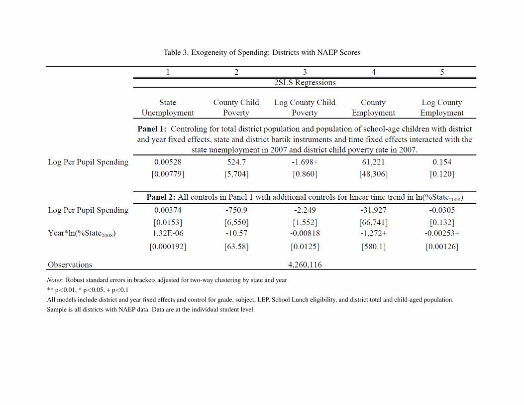
Table 3. Exogeneity of Spending: Districts with NAEP Scores

Notes: Robust standard errors in brackets adjusted for two-way clustering by state and year** p<0.01, * p<0.05, + p<0.1All models include district and year fixed effects and control for grade, subject, LEP, School Lunch eligibility, and district total and child-aged population.Sample is all districts with NAEP data. Data are at the individual student level.

Table 4. Two-Stage-Least-Squares Regressions: School Spending Categories

Notes: Robust standard errors in brackets adjusted for two-way clustering by state and year** p<0.01, * p<0.05, + p<0.1All models control for total district population and population of school-age children with district and year fixed effects, state and district Bartik instruments and timefixed effects interacted with the state unemployment in 2007 and district child poverty rate in 2007 and additional controls for linear time trend in ln(%State2008).Sample is all available districts. Regression models are weighted by Public School Enrollment.a. Other spending includes Non Elem/Sec and Payments.

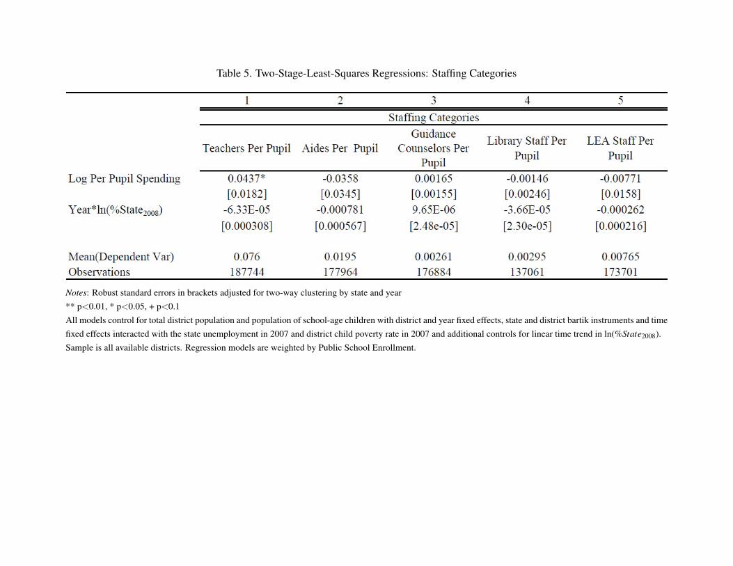
Table 5. Two-Stage-Least-Squares Regressions: Staffing Categories

Notes: Robust standard errors in brackets adjusted for two-way clustering by state and year** p<0.01, * p<0.05, + p<0.1All models control for total district population and population of school-age children with district and year fixed effects, state and district bartik instruments and timefixed effects interacted with the state unemployment in 2007 and district child poverty rate in 2007 and additional controls for linear time trend in ln(%State2008).Sample is all available districts. Regression models are weighted by Public School Enrollment.

Table 6. Two-Stage-Least-Squares Regressions. Districts with NAEP Scores

Notes: Robust standard errors in brackets adjusted for two-way clustering by state and year** p<0.01, * p<0.05, + p<0.1All model control for total district population and population of school-age children with district and year fixed effects (Basic controls), student grade, subject, LEPand Free/Reduced Lunch eligibility. Full controls also include state and district Bartik instruments and time fixed effects interacted with the state unemployment in2007 and district child poverty rate in 2007. Economic variables include the state unemployment rate, the district average annual employment and the number ofchildren living in poverty in the district.Sample is all available NAEP observations linked to districts.

Table 7. Two-Stage-Least-Squares Regressions: By Subject and Grade.

All models control for total district population and population of school-age children with district and year fixed effects student grade, subject, LEP and Free/ReducedLunch eligibility, state and district Bartik instruments and time fixed effects interacted with the state unemployment in 2007 and district child poverty rate in 2007and additional controls for linear time trend in ln(%State2008).Sample is all available NAEP observations linked to districts.

Table 8. 2SLS Regressions: Public and Private School State Averages

Notes: Robust standard errors in brackets adjusted for two-way clustering by state and year** p<0.01, * p<0.05, + p<0.1All model control for total district population and population of school-age children with district and year fixed effects (Basic controls) and average student grade,subject, LEP and Free/Reduced Lunch eligibility. Full controls also include the Bartik instrument and time fixed effects interacted with the state unemployment in2007 and district child poverty rate in 2007 and additional controls for linear time trend in ln(% State2008). Economic variables include the state unemployment rate,the district average annual employment and the number of children living in poverty in the district.

Table 9. Two-Stage-Least-Squares Regressions: High School Completion Rates (IPUMS)

Notes: Robust standard errors in brackets adjusted for two-way clustering by state and year** p<0.01, * p<0.05, + p<0.1All models control for total district population and population of school-age children with district and year fixed effects (Basic controls). Full controls also includestate and district Bartik instruments and time fixed effects interacted with the state unemployment in 2007 and district child poverty rate in 2007. Economic variablesinclude the state unemployment rate, the district average annual employment and the number of children living in poverty in the district.

Appendix

A Data on School Spending and ResourcesThe data on district level school finances is collected from the Census website.17 The underlying data comes from

the Common Core of Data (CCD) School District Finance Survey (F-33). It consists of data submitted annually to theNational Center for Education Statistics (NCES) by state education agencies (SEAs) in the 50 states and the Districtof Columbia. The purpose of the survey is to provide finance data for all local education agencies (LEAs) that providefree public elementary and secondary education in the United States. Both NCES and the Governments Division of theU.S. Census Bureau collect public school system finance data, and they collaborate in their efforts to gather these data.The F-33 data provides information on revenues, expenditures, and the number of students enrolled. Expendituresare reported in a number of categories including instructional spending, capital outlays, and administrative spending.Revenues are reported in several fine categories and aggregated to local, state, and federal sources.

The surveys are administered annually from 1992 onward. We link together multiple years of data to create abalanced panel school district data set for analysis. In constructing the data set, we found that the financial datacontained some extremely large and small values. These values could be valid, but it is more likely that some districtsincorrectly reported enrollments or expenditures. We therefore censored the data by deleting extreme values. First, wecalculated the (unweighted) 99th and 1st percentile district in total per-pupil current expenditures for each state andyear. We then capped values of districts with per-pupil expenditures at greater than 200 per-cent of the 99th percentileof per-pupil revenues or less than 50 percent of the 1st percentile.

For school spending categories (such as capital or instructional salaries), we replace values with missing where thecpi-adjusted per-student categorical spending value is more than twice the 99th percentile. We follow a similar strategyfor reported staffing categories, which come from the NCES Common Core of Data LEA Universe surveys (CCD),replacing staffing values with missing if the total staffing variable or the staffing per student (or students per staff) ismore than twice the 99th percentile.

B Recession Intensity & Employment DataImportant to our identification strategy is controlling for the direct effect of broader recessionary economic condi-

tions. For this purpose, we construct an index of recession severity and exposure. We exploit the fact that the impact ofrecession varied on basis of local industrial compositions and create a shift-share instrument, along the lines of Bartik(1991), which captures changes in economic conditions attributable to the onset of the recession.

To do so, we follow the steps broadly outlined in Yagan (2017). We retrieve average annual county-level employ-ment data from the Quarterly Census of Employment and Wages (QCEW).18 Each county’s time-varying shift-shareshock is computed as the projected unemployment in each year, based on the interaction between the 2007, pre-recession, employment composition by two-digit NAICS industry categories and the nationwide unemployment by thesame groupings in that year. Formally, in county c during year t the instrument equals:

17For instance, data for the school year 2015-2016 is available at https://www.census.gov/data/tables/2015/econ/school-finances/secondary-education-finance.html and data for the other years can be re-trieved by modifying the appropriate part of the url.

18The QCEW program publishes an annual count of employment and wages reported by employers covering 98 per-cent of U.S. jobs, available at the county, MSA, state and national levels by industry. Average annual data were down-loaded from the Bureau of Labor Statistics for each county and year from https://www.bls.gov/cew/datatoc.

htm

Bartik Predictorct = ∑j

(E jc2007

∑ j′ E j′c2007×National Unemployment jct

)(10)

where j denotes a two-digit industry, E jc2007 denotes total employment in industry j in county c in 2007, andNational Unemployment jt is the nationwide unemployment rate in industry j in county c in year t.

From the same dataset (QCEW) above, we also compile the annual total employment number in each county as anadditional measure of economic status.

To utilize these controls in the analysis, we merged the county level data on recession shock to schools to the database to district level data from the Common Core and F33 outlined above. It is not straight forward to match the recordssince the district to county mapping is not one to one. To overcome this complication, we use a spatial correspondencefile from http://mcdc.missouri.edu/websas/geocorr12.html. This file identifies the exact percentage of adistrict’s area contained in each county. Using this information, we link the district level observations to the weightedaverage of values in the counties that the district overlaps. The resulting value approximates the shift-share predictorin the district, assuming industrial compositions are distributed uniformly within each county.

C NAEP DataWe use restricted-use individual-level NAEP test score data from the National Center for Education Statistics. We

infix the raw files to Stata, including all plausible score values per student, and restricting the sample to the NAEPreporting sample and public school students, except in the case of our robustness test, which includes private schoolstudents as well. The restriction to the reporting sample and public school students corresponds directly to the sampleused to calculate state averages as reported publicly by NCES.

We link student scores to school districts using the reported NCES school identifier. Our dependent variable in allNAEP estimations is the mean of all reported plausible values for each student, year, grade, and subject, standardized tothe base year of 2003. We restrict our analyses to the years 2002 and later, as NAEP sampling increased dramaticallyafter 2001 and testing years became more consistent at this time. In data that are aggregated to the state level, weweight the state-averages by the reported original weight, ORIGWT.

Appendix Table 1: NAEP Availability

4th Grade 8th Grade 4th Grade 8th Grade TestedYear Math Math Reading Reading Students2015 X X X X 43043820142013 X X X X 57529820122011 X X X X 61978920102009 X X X X 57130820082007 X X X X 62022020062005 X X X X 58945820042003 X X X X 6422442002 X X 24022820012000 X X X 2224619991998 X X 1539119971996 X X 1080519951994 X 603019931992 X X X 16719

Notes: NAEP availability by subject-grade in sample.

Appendix Figure 1. Fraction of Education Revenue from State Sources

Notes: This map shows the extent of variation in (%)States across the country.

Appendix Figure 2. Marginal Effect of IV on Staffing Ratio.All Districts

Notes: The dashed connected line depicts the coefficients on the individual calendar year indicators interacted with thestate reliance on state revenue in 2008, lnΩs. More specifically, it plots the βt for each calendar year from Equation6) relative to the coefficient for 2007. The gray area depicts the 90 percent confidence interval for each individualcalendar year interaction. The solid lines represent the linear fit during the pre-recession period (negative values ofexposure) and post recession periods (non-negative values of exposure).

Appendix Figure 3. Marginal Effect of IV by Year on Per-Pupil Spending (Between ages 15 to 18)−

.1−

.05

0.0

5

−5 −4 −3 −2 −1 0 1 2 3 4 5 6 7School age Years of Exposure to the Recession

Notes: The connected dashed lines represents the individual exposure year interaction coefficients (relative to the effectfor 2007). The gray area depicts the 90 percent confidence interval for each individual exposure year interaction. Thesolid lines represent the linear fit during the pre-recession period (negative values of exposure) and post recessionperiods (non-negative values of exposure).