wp7 – demo-site implementation deliverable d.7.3
TRANSCRIPT

Funded by:
European CommissionFramework Programme 7
Cooperation
Thematic AreaEnvironment 6.4Earth Observation and assessment tools for sustainable development
WP7 – Demo-Site imPlementation
Deliverable D.7.3rePort on roSia montana CaSe StuDy inveStigationS – verSion 2
Compiled byCalin Baciu - UBB, Universitatea Babes Bolyai, RomaniaMarc Goossens - Geosense B.V., the NetherlandsIls Reusen - VITO, Flemish Institute for Technological Research, BelgiumCarolien Tote - VITO, Flemish Institute for Technological Research, BelgiumStephanie Delalieux - VITO, Flemish Institute for Technological Research, BelgiumDries Raymaekers - VITO, Flemish Institute for Technological Research, BelgiumCristina Dobrota - UBB, Universitatea Babes Bolyai, RomaniaCristian Pop - UBB, Universitatea Babes Bolyai, RomaniaIldiko Varga - UBB, Universitatea Babes Bolyai, RomaniaCarmen Roba - UBB, Universitatea Babes Bolyai, RomaniaDan Costin - UBB, Universitatea Babes Bolyai, RomaniaAmer Smailbegovic - Photon llc., Croatia
Submitted by: GEONARDO Environmental Technologies Ltd.(Project Coordinator)
Project Coordinator name: Mr. Peter Gyuris
Project Coordinator organization name: GEONARDO, Hungary
www.impactmin.eu
IMPACT MONITORING OF MINERAL RESOURCES ExPLOITATION
ContraCt nº
2 4 4 1 6 6

This report has been submitted to the European Commission for evaluation and for approval.
Currently the content of this report does not reflect the official opinion of the European Union.
Responsibility for the information and views expressed in the report therein lies entirely with the
author(s).

IMPACTMIN WP7.3 Contract №: 244166
2
Executive summary Rosia Montana is one of the most representatives gold deposits in Europe, with a long history of mining, spanning over the last two millennia. The currently known and inferred reserves are exceeding 300 tonnes of gold and 1500 tonnes of silver. The mining activity has ceased in 2006 due to economic reasons. Very few remediation actions have been implemented in the area since the mining was stopped. A very large scale new mining project is proposed by Rosia Montana Gold Corporation (RMGC). Choosing Rosia Montana as a demonstration site has been a very good decision, as the ImpactMin project has been implemented during the inactivity period between the moment 2006 and a potential restart of mining. The damage to the environment produced by the two millennia of mining is significant. About 140 km of galleries and two open pits, with the associated waste dumps and tailings depots are the main mining features in the area. The landscape has been considerably modified, especially by the open pit works. The main source of pollution that is currently active is the acid mine drainage (AMD), produced by the exposed rock surfaces in underground galleries and in open pits. Important sources of acidic waters are also the waste dumps and the tailings management facilities. Our study was mainly focused on environmental components that can be observed by remote sensing technology. In this regard, we took into account the characteristics of soils and the stress induced by pollution on vegetation. A combination of investigation means has been used, including ground hyperspectral measurements on soil and vegetation, high-resolution multispectral satellite imagery, UAV imagery, airborne hyperspectral imagery, together with chemical analyses of soils and stream sediments, and chemical analyses on tree leaves. The contents of Cd, Cr, Cu, Ni, Pb, and Zn have been measured in soils and vegetation. The soils in the area are predominantly acidic, and to a much lower extent neutral or alkaline. The level of contamination of soils with heavy metals is low, excepting the proximity of the mine, and it is mainly related to the geochemical background of the area. Pronounced contamination has been observed in the stream sediments samples along the AMD pathways. Two tree species, birch (Betula pendula) and hornbeam (Carpinus betulus) have been studied regarding the heavy metals content in leaves and the spectral response. The concentrations of heavy metals in leaves are generally low. The remarkable ability of birch to uptake zinc has been noticed. A series of Worldview-2 multispectral images from three consecutive years, during the same season, has been used for a multi-temporal analysis, with the scope to assess the normal variability of the surface characteristics. A low altitude hyperspectral (VNIR) survey has been performed, covering the mining area and its surroundings at 50 cm resolution. The two approaches have highlighted the inhomogeneity and complexity of Rosia Montana area from the point of view of remote sensing. Consequently, it was decided to use a Smartplanes UAV in order to acquire ultra-high-resolution aerial photographs, with the aim to facilitate the integrated interpretation of field data, hyperspectral and Worldview-2 imagery. Special attention has been paid to the grasslands, that are covering about 70% of the study area. We assume that the environmental degradation will have a negative effect on the herbaceous cover, mainly expressed as lower vegetation density. This will lead to enhanced erosion, and stronger deterioration of the grasslands. The airborne hyperspectral data has been mainly used for testing the vegetation stress as proxy for pollution. Four indices were found to be useful for discriminating the polluted from non-polluted areas: Photochemical Reflectance Index (PRI), Normalised Pigment Chlorophyll Ratio Index (NPCI), Simple Ratio Pigment Index (SRPI), and Stress-related Index (SR). Our investigations have shown that the local environment has reached a steady state, with relatively minor changes from one year to the other. Under these circumstances, our approach adds important elements to the baseline of possible future mining operations, and also documents innovative techniques for observing the subtle gradual changes that can be associated with the environmental degradation related to mining. These investigation methods are complementing the classical approach that is currently implemented in mining and industrial areas for the environmental assessment.

IMPACTMIN WP7.3 Contract №: 244166
3
TABLE OF CONTENTS
LIST OF FIGURES ........................................................................................................................ 5
LIST OF TABLES ........................................................................................................................ 10
1 INTRODUCTION ................................................................................................................. 11
1.1 Aims and objectives ............................................................................................................. 11
1.2 Approach and collaborative work ..................................................................................... 13 1.2.1 Tasks carried out by GEONARDO ................................................................................................. 13 1.2.2 Tasks carried out by UBB ............................................................................................................... 13 1.2.3 Tasks carried out by GEOSENSE ................................................................................................... 13 1.2.4 Tasks carried out by VITO .............................................................................................................. 14 1.2.5 Tasks carried out by Photon ............................................................................................................ 14 1.2.6 Contributions of stakeholders .......................................................................................................... 14
2 BACKGROUND DATA ......................................................................................................... 15
2.1 Environmental data ............................................................................................................. 15
2.2 Remote sensing data ............................................................................................................ 16
3 STATE OF THE ENVIRONMENT AND RELATION WITH THE MINING ACTIVITY ................. 19
3.1 Geological setting ................................................................................................................. 19
3.2 Soils and sediments .............................................................................................................. 23 3.2.1 The soil cover .................................................................................................................................. 23 3.2.2 Stream sediments ............................................................................................................................ 26
3.3 Water .................................................................................................................................... 28 3.3.1 Surface water ................................................................................................................................... 28 3.3.2 Groundwater .................................................................................................................................... 33
3.4 Mining in Rosia Montana area ........................................................................................... 34
3.5 Mining waste ........................................................................................................................ 40
4 CHEMICAL CHARACTERISTICS OF SOIL AND VEGETATION ............................................. 46
4.1 Sample collection, preservation, and handling ................................................................. 46 4.1.1 Soils sampling strategy.................................................................................................................... 46 4.1.2 Soil and sediment samples collection and processing ..................................................................... 48 4.1.3 Leaves ............................................................................................................................................. 49
4.2 Sample analysis .................................................................................................................... 50 4.2.1 Measurement of the soil pH ............................................................................................................ 50 4.2.2 Determination of the heavy metals contents in soils and sediments by Flame Atomic Absorption
Spectrometry (FAAS)................................................................................................................................... 51 4.2.3 Determination of heavy metals in vegetation by Inductively Coupled Plasma – Mass Spectrometry
(ICP-MS) ...................................................................................................................................................... 55 4.2.4 Determination of chlorophyll content and fluorescence in leaves ................................................... 58
4.3 Results of soils and sediments chemical analyses ............................................................. 64
4.4 Results of chemical analyses on leaves............................................................................... 68
4.5 Results of the chlorophyll content and fluorescence measurements ............................... 74
5 HYPERSPECTRAL MEASUREMENTS AND REMOTE SENSING ............................................. 76
5.1 Overview .............................................................................................................................. 76
5.2 Field work ............................................................................................................................ 79 5.2.1 Field campaign 2011 ....................................................................................................................... 79

IMPACTMIN WP7.3 Contract №: 244166
4
5.2.2 Field campaign 2012 ....................................................................................................................... 88
5.3 Preprocessing of WorldView 2 imagery ............................................................................ 89
5.4 Processing of Smartplanes imagery ................................................................................... 93
5.5 Airborne hyperspectral survey .......................................................................................... 93
5.6 Airborne data quality assessment ...................................................................................... 96 5.6.1 Quality of the geometric correction ................................................................................................. 96 5.6.2 Quality of the radiometric correction .............................................................................................. 96
6 INTERPRETATION OF RESULTS OF THE HYPERSPECTRAL MEASUREMENTS AND REMOTE
SENSING .................................................................................................................................. 102
6.1 Interpretation of sediments, soils and rocks characteristics .......................................... 102 6.1.1 Stream sediments spectra .............................................................................................................. 102 6.1.2 Soil and rock spectra ..................................................................................................................... 104 6.1.3 Soil chemistry................................................................................................................................ 107 6.1.4 Mapping soil and grassland variations using the Worldview2 imagery ........................................ 109 6.1.5 Image classification of soils .......................................................................................................... 118 6.1.6 Time series analysis and temporal monitoring .............................................................................. 125 6.1.7 Hyperspectral mapping of soils ..................................................................................................... 128 6.1.8 The pseudo-hyperspectral evaluation ............................................................................................ 133 6.1.9 Cost-benefit considerations ........................................................................................................... 138
6.2 Monitoring vegetation stress ............................................................................................ 139 6.2.1 Monitoring vegetation stress – leaf level....................................................................................... 139 6.2.2 Monitoring vegetation stress – airborne level ............................................................................... 144 6.2.3 Outlook .......................................................................................................................................... 151
7 CONCLUSIONS ................................................................................................................. 152
8 REFERENCES ................................................................................................................... 154

IMPACTMIN WP7.3 Contract №: 244166
5
List of figures
Figure 3-1. Position of the study area within the Golden Quadrilateral ................................................................ 20
Figure 3-2. Geologic map and cross section of Rosia Montana gold deposit (RMGC, 2006). ............................. 21
Figure 3-3. Dacite rocks with remains of the old mining works in (a) Carnic Massif, and (b, c, d) Jig-Vaidoaia
area. ................................................................................................................................................. 22
Figure 3-4. Black breccia (dark coloured) and dacite (light coloured) in Carnic Massif. ..................................... 22
Figure 3-5. Piatra despicata (left) and Piatra Corbului (right) nature monuments in Carnic area....................... 22
Figure 3-6. Tridimensional model of the gold deposit in Rosia Montana (RMGC, 2006).................................... 23
Figure 3-7. Soil profile in Rosia Montana area. .................................................................................................... 25
Figure 3-8. Stream sediments affected by AMD, Rosia Montana area. ................................................................ 26
Figure 3-9. Concentrations of heavy metals and As in river sediments in Abrud/Aries catchment, as a function of
distance from source of the River Abrud (fluvio, 2004). ................................................................. 27
Figure 3-10. The water sampling network in Rosia Montana area, operated by RMGC. ..................................... 29
Figure 3-11. Artificial lakes in Rosia Montana area: (a) Taul Mare; (b) Taul Brazi. ............................................ 31
Figure 3-12. (a) Acid mine drainage downstream of Saliste tailings dam; (b) Fe-hydroxides and gypsum in the
seepage area, Saliste tailings dam; (c) Weir on Saliste Valley, close to the confluence with Abrud
River. (d) Mixing between the AMD-polluted waters of Abrud River (left) and the relatively clean
waters of Aries River (downstream Campeni). ................................................................................ 32
Figure 3-13. Conceptual hydrogeologic model for Rosia Montana area (MWH, 2007) ....................................... 34
Figure 3-14. (a) Entrance to the Roman gallery in Orlea mine; (b) Reproduction of the text of tabula cerata
XVIII; (c) and (d) Roman gallery in Orlea mine. ............................................................................ 36
Figure 3-15. Archeological heritage in Rosia Montana. (a) Tombstone, (b) small monument dedicated to God
Iannus (Roman period). (c) Ore grinding and (d) gold panning technique (first half of 20th century;
photo collection Bazil Roman). ....................................................................................................... 37
Figure 3-16. The network of underground works in Rosia Montana. ................................................................... 37
Figure 3-17. Rosia Montana mining area (red polygon). ...................................................................................... 38
Figure 3-18. Cetate open pit; no current mining activity. ..................................................................................... 39
Figure 3-19. Cetate open pit. Carnic Masif with Carnic open pit in the background. ........................................... 39
Figure 3-20. Distribution of the ore grade (gold g/t) in the four mining fields in Rosia Montana area (RMGC,
2006). ............................................................................................................................................... 40
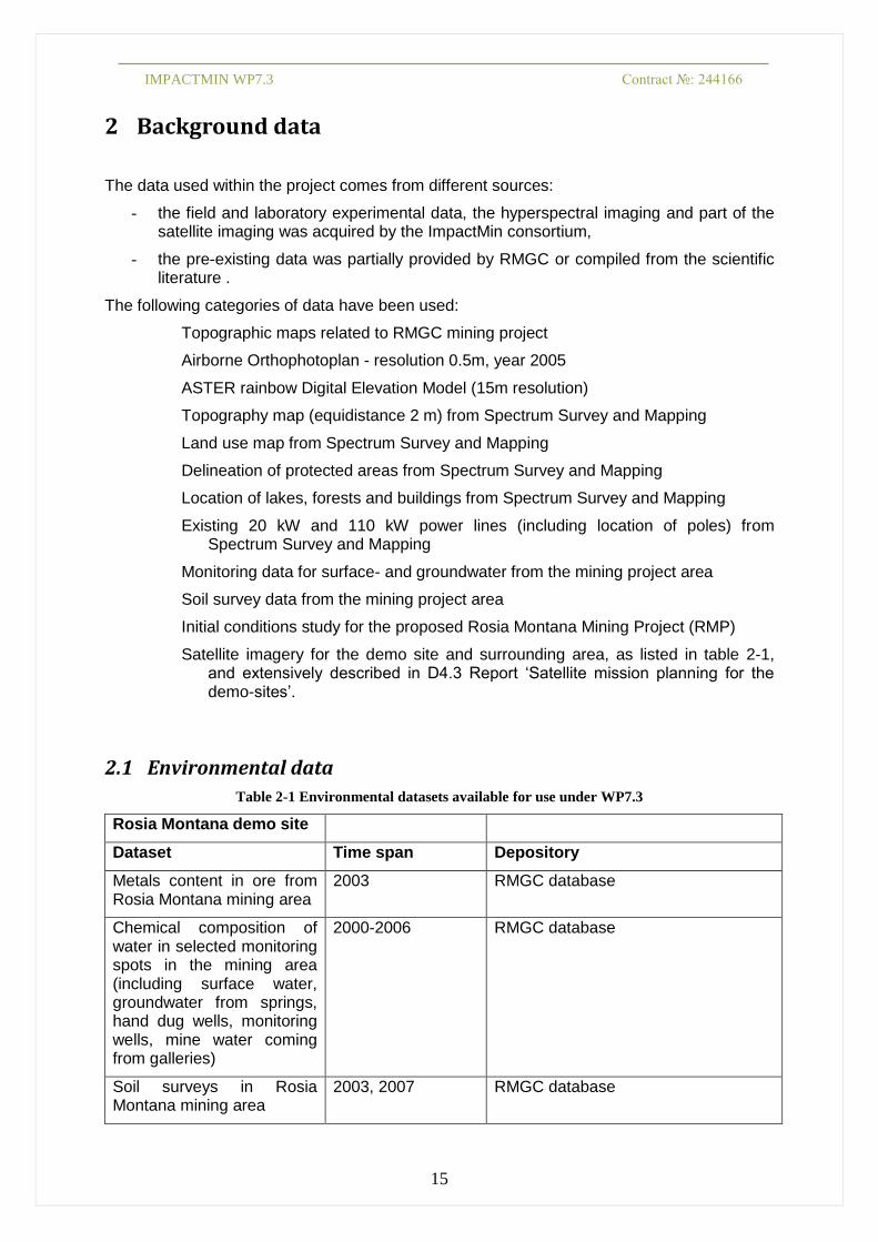
Figure 3-21. Waste dumps in Orlea area. .............................................................................................................. 41
Figure 3-22. Valea Verde waste dump. south of Cetate open pit. ......................................................................... 41
Figure 3-23. Gura Rosiei tailings pond (a) before reclamation and (b) during the reclamation works. ................ 43
Figure 3-24. The acid drainage test site. ............................................................................................................... 45
Figure 3-25. Plastic barrels with rock samples used for the kinetic test................................................................ 45
Figure 4-1. Different categories of soil exposures. Soils in the mineralized areas (a, b), in scarps, road cuts etc
(c), in uncut grasslands (d), in recently cut grassland (e), in grazing lands with molehills (f), in
grazing land with decreasing vegetation density (g-i). .................................................................... 47
Figure 4-2. Location of soil samples taken during the respective field campaigns for spectral analysis with
contact probe.................................................................................................................................... 48
Figure 4-3. Soils/sediments samples processed for digestion. .............................................................................. 49
Figure 4-4. The pH measurement in soil/sediment samples. ................................................................................. 50
Figure 4-5. Multiparameter device used for pH measurements. ........................................................................... 50
Figure 4-6. Soil/sediment sample digestion. ......................................................................................................... 51

IMPACTMIN WP7.3 Contract №: 244166
6
Figure 4-7. FAAS system. ..................................................................................................................................... 52
Figure 4-8. Calibration curves of the investigated metals. .................................................................................... 53
Figure 4-9. Vegetation samples processed for digestion. ...................................................................................... 55
Figure 4-10. Samples digestion (left: during digestion; right: after digestion). .................................................... 56
Figure 4-11. ICP-MS system................................................................................................................................. 57
Figure 4-12. Opti Sciences CCM 200 chlorophyll-meter. .................................................................................... 60
Figure 4-13. Leaf samples prepared for analysis .................................................................................................. 61
Figure 4-14. The process of heating and separation using FALC Heating Mantles. ............................................. 61
Figure 4-15. Metertek SP-850 spectrophotometer ................................................................................................ 62
Figure 4-16. OPTI SCIENCES – OS1–FL fluorometer ........................................................................................ 64
Figure 4-17. Soil sampling in Jig area. ................................................................................................................. 64
Figure 4-18. Spatial distribution of the soil pH values in the study area (left) and frequency (right). .................. 65
Figure 4-19. Concentrations of heavy metals in soils and stream sediments: (a) Cu concentrations; (b) Pb
concentrations; (c) Cd concentrations; (d) Zn concentrations; (e) Cr concentrations; (f) Ni
concentrations. ................................................................................................................................. 67
Figure 4-20. Frequency of the heavy metals contents in soils and stream sediments samples. ............................. 68
Figure 4-21. Heavy metals contents in leaves: (a) Cr in birch leaves; (b) Cr in hornbeam leaves; (c) Cu in birch
leaves; (d) Cu in hornbeam leaves; (e) Ni in birch leaves; (f) Ni in hornbeam leaves; (g) Pb in birch
leaves; (h) Pb in hornbeam leaves; (i) Cd in birch leaves; (j) Cd in hornbeam leaves; (k) Zn in birch
leaves; (l) Zn in hornbeam leaves. ................................................................................................... 71
Figure 4-22. Heavy metals contents in birch leaves compared to soil. ................................................................. 72
Figure 4-23. Heavy metals contents in hornbeam leaves compared to soil. .......................................................... 73
Figure 4-24. Chlorophyll content and fluorescence values in birch and hornbeam leaves. .................................. 75
Figure 5-1. Overview of the Rosia Montana deposit, showing the various open pits and waste dumps. .............. 76
Figure 5-2. 3-D overview of the Saliste tailings dam, generated from Smartplanes aerial photography. ............. 76
Figure 5-3. Acid drainage with Iron-rich chemical precipitate. ............................................................................ 77
Figure 5-4. Proposed mining infrastructure showing the future open pits in green. Past mining areas are located
within the boundaries of the future open pits. .................................................................................. 78
Figure 5-5. Locations of spectral samples from field campaigns 2011/2012. Red polygons indicate the
approximate outlines of the pits planned by RMGC, the yellow dashed line indicates the limit of the
Industrial Protection Area. A selection of the leaf and soil samples was used for chemical analysis.
......................................................................................................................................................... 78
Figure 5-6. Traditional small-scale farming that is typical for this region. Cutting the grass is still done manually
using a scythe................................................................................................................................... 79
Figure 5-7. Locations of spectral samples from field campaign 2011. Red polygons indicate the approximate
outlines of the pits planned by RMGC, the yellow dashed line indicates the limit of the Industrial
Protection Area. ............................................................................................................................... 80
Figure 5-8. Hyperspectral measurements of soil samples by the ASD spectrometer in the lab. ........................... 81
Figure 5-9. Hyperspectral measurements on leaves in the field ............................................................................ 81
Figure 5-10. A) Natural colour composite of the 2010 WV2 image, illustrating the differences in greenness of the
grasslands. Arrows indicate examples of typical areas with different vegetation density. The image
corresponds with the yellow outline on the lower two images. B) Land classification of the WV2-
2010 image. The colours of the classes correspond with the colours of the arrows. C) Land
classification of the WV-2011 image, using the same NDVI-thresholds as for the 2010 image. .... 82
Figure 5-11. Plot of Red-edge position for Birch leaves sampled in the 2011 field campaign. The spectral plot
shows some typical reflectance spectra for Birch leaves. ................................................................ 84

IMPACTMIN WP7.3 Contract №: 244166
7
Figure 5-12. Comparison of Worldview2 Multispectral (2m resolution), WV2-pansharpened multispectral (50
cm resolution), Hyperspectral VNIR (50 cm resolution) and Smartplanes image (4 cm resolution.
The red arrows point to the location of the soil exposure shown in the photograph. This type of soil
exposure is found frequently in grass lands used for grazing. ......................................................... 86
Figure 5-13. Location of Saliste tailings dam and Cetate pit. ............................................................................... 87
Figure 5-14. Sample locations in the main pit of Rosia Montana Mine: Cetate ................................................... 87
Figure 5-15. Sampling in Cetate Pit ...................................................................................................................... 87
Figure 5-16. Sampling at Saliste tailings dam ....................................................................................................... 88
Figure 5-17. Planned locations of sample profiles for the May-2012 field campaign (blue) and location of the
Smartplanes UAV survey blocks (red) ............................................................................................ 89
Figure 5-18. Scattergrams showing the relation (after atmospheric correction) of respectively bands 1,5 and 8 of
WV2-2012 (horizontal axes) with WV2-2011 (vertical axes, figs a, b, c) and with WV2-2010
(vertical axes, figs d, e and f). The red lines indicate r=1. ............................................................... 91
Figure 5-19. a. WordView-2 image, b. Habitat map, c. forest species highlighted on the habitat map, d. classified
WV2 map indicating different forest species, e. grasslands and meadows highlighted on the habitat
map, f. classified WV2 image of grasslands and meadows indicating different LAI values ........... 92
Figure 5-20. Hyperspectral strips projected on the WV-2 natural colour image, showing the coverage of the
hyperspectral survey (red) and of the Smartplanes survey blocks (blue outlines). .......................... 94
Figure 5-21. Location of spectral measurements of ground targets and leaves ..................................................... 96
Figure 5-22. Comparison of the ATCOR vs FODIS atmospheric correction over an asphalt target. ................... 97
Figure 5-23. Ground reference targets identified in the AISA EAGLE dataset .................................................... 97
Figure 5-24. Spectra of the ground reference targets measured with the ASD ..................................................... 98
Figure 5-25. Results of the intercomparison between the ground measurements (ASD and Spectral evolution)
and the AISA EAGLE data. ............................................................................................................. 99
Figure 5-26. Comparison of two adjacent flight lines ......................................................................................... 100
Figure 5-27. Spectral comparison of two adjacent flightlines on 6 targets. ........................................................ 101
Figure 6-1. Plots of the spectral Iron-oxide index, pH, Lead –content and Copper content of the stream sediments
around the deposit. ......................................................................................................................... 103
Figure 6-2. Plots of pH, Cd, Pb, Zn, Cu and Ni in stream sediments against the ratio of spectral reflectances at
759 and 937 nanometers. ............................................................................................................... 103
Figure 6-3. Typical example of rock outcrops around the deposit (a, b and c), and other outcrops, such as
individual boulders (d), scarps (e) and landslides (f). .................................................................... 104
Figure 6-4. Maps showing the presence of minerals in soil and rock samples that are possibly related to the
formation of the deposits. (a) illite, (b) kaolinite, (c) goethite and (d) jarosite. ............................. 105
Figure 6-5. Depth of the 900-nm feature (left) using the ratio of bands750 nm/900 nm, and of the 2200 nm
feature (right). For the 900 nm-feature we have resampled to the corresponding WV2-
bandpositions. Depth of the 2200 nm-feature has been computed on the basis of the relative depth
in the hulled-spectrum using The Spectral Geologist (TSG). At the top we have plotted lab-spectra
for the relevant minerals that show absorption features at these wavelengths. .............................. 106
Figure 6-6. Plots of the spatial distribution of (a) Copper, (b) Lead, (c) Zinc, (d) Cadmium, (e) Chrome and (f)
pH. ................................................................................................................................................. 107
Figure 6-7. Relationship between (a-f) the spectral Iron-oxide index (WV6/WV8) and some relevant chemical
parameters, and between (g-l) the depth of the 2200 nm absorption feature and the chemical
parameters. The blue symbols represent the (regional) samples collected in May 2012, and the red
symbols represent samples collected in 2011 on or near the deposits. .......................................... 108
Figure 6-8. Plots showing the relation between the spectra from contact probe samples and the Worldview2-
spectra for the corresponding image pixels. In order to correlate the contact probe spectra with the
WV2-spectra, the former have been resampled to the respective WV2 band positions. Rock

IMPACTMIN WP7.3 Contract №: 244166
8
samples 2011 are mostly taken from locations in or near the deposits. Soil samples 2011 are also
taken mostly at or near the deposits. Soil samples May 2012 are regional soil samples, collected on
profiles in grasslands. Soil samples July 2012 are taken in the transitional zone between the May
2012 and the 2011 soil samples, mostly from fairly well exposed soils. ....................................... 111
Figure 6-9. Comparison of band ratios for contact probe spectra and WV2-spectra. These are band ratios that are
often considered useful to map subtle variations in WV2-imagery. The symbols are the same as in
figure 29. For a better understanding of the meaning of the band-ratios, we have added a plot with
the WV2-spectra for representative surface materials. These spectra have been obtained by
resampling USGS-reference library spectra to WV2- band positions. .......................................... 112
Figure 6-10. Locations of solar reflectance measurements collected between June 22 and July 4, 2012, and the
locations where samples were taken for contact probe analysis. In this plot we made a distinction
between solar reflectance targets that consisted for more than 90% of exposed soil with minor
grass, and (grassland) targets with a ratio between 0% and 90% exposed soil. ............................. 113
Figure 6-11. Plots showing the relation between the solar reflectance spectra collected for soils and rocks in July
2012 and the Worldview2-spectra for the corresponding image pixels. In order to correlate the
spectroradiometer spectra with the WV2-spectra, the former have been resampled to the respective
WV2 band positions. ..................................................................................................................... 114
Figure 6-12. Comparison of band ratios for solar reflectance spectra and WV2-spectra. These are band ratios that
are often considered useful to map subtle variations in WV2-imagery. The symbols are the same as
in figure 32. For a better understanding of the meaning of the band-ratios, we have added a plot
with the WV2-spectra for representative surface materials. These spectra have been obtained by
resampling USGS-reference library spectra to WV2- band positions. .......................................... 116
Figure 6-13. Spectral mixtures for different types of grasslands: a) Long green grass with different proportions of
soil exposed; b) Recently cut green grassland with different proportion of soil exposed; c) Recently
cut grassland with different proportions of dry grass; d) Grazing land with short grass and different
proportions of soil exposed. ........................................................................................................... 117
Figure 6-14. Comparison of the July 2012 WV2 imagery and the Smartplanes imagery for various types of soil
exposures a-b: red arrows mark examples of recently cut, and dried grasslands. Hay stacks are
clearly visible on the Smartplanes image; Blue arrows indicate exposed soil in a crop field. c-d:
Red arrows mark examples areas that appear to be in the process of being cut. Blue arrows mark
examples of exposed soil. .............................................................................................................. 119
Figure 6-15 e-f: The red arrows mark a strange zoning in the grasslands for the WV2-image. This zoning is not
visible in the Smartplanes image. We suspect that in this area the cutting of the grass is still in
progress, and that in the brown areas grass has been cut in the four days lapse between the
acquisitions of the two datasets, whereas the greener part has probably been cut more recently. The
blue arrows mark exposure of rocks and soil. g-h: image of typical grazing land with very short
grass, and many small spots with exposed soil (see also figure 6-12. The blue arrow marks a small
pile of gravel. The other white spot on the Smartplanes image is our field-van. ........................... 120
Figure 6-16. Results of the WorldView2 land-cover classification using the NDVI. Arrows mark the locations
discussed in the previous section. For explanation of the colours, see text above. ........................ 121
Figure 6-17. WV2 band ratio (6/8) results for the 2012-image for soil class 1 (bare soils, top) and soil class 1 and
2 (bare soils and scarce vegetation respectively, bottom). ............................................................. 123
Figure 6-18. Field spectra were resampled to WV2-bands, and the plots show the ratio of the WV6/WV8 for the
solar spectra (top) and for the contact probe spectra (bottom) overlain on the same ratio for the
WV2-image. The same colour scheme has been used for the image data and the field spectra. ... 124
Figure 6-19. Distribution of soil classes for 2012 (a), 2011 (b) and 2010 (c).By combining a specific soil class
for each year into an RGB colour composite we can visualize the changes for a specific soil class
over time (figs. d-g). Fig. d: (Red) distribution of bare soil in 2012, (green) distribution of bare soil
in 2011, (blue) distribution of bare soil in 2010. Fig. e: same for the second class (soils with some
vegetation). Fig. f: same for the third class (soils with significant vegetation). Fig. g: same for the
fourth class (mostly vegetation with some soil)............................................................................. 126
Figure 6-20. Difference of the Ratio WV6/WV8 between 2010 and 2012 for bare soils (top) and soils with some
grass-cover (bottom). Higher values indicate an increase of Fe-oxide content in 2012 compared to
2010. .............................................................................................................................................. 127

IMPACTMIN WP7.3 Contract №: 244166
9
Figure 6-21. Left: comparison of WV2-pixel signatures with corresponding field spectra; Right: comparison of
AISA-Eagle pixel signatures with corresponding field spectra. .................................................... 128
Figure 6-22. Top: Results of Spectral Angle classification for Smartplanes imagery. Red pixels represent
exposed bare soils. Bottom: Results of bare coil classification using for WV2 (blue pixels) and
hyperspectral (red pixels), based on thresholding of the NDVI. The grid interval is 50m. ........... 129
Figure 6-23. Spectra of Jarosite and Goethite from the USGS- spectral library and AISA-EAGLE imagery. ... 130
Figure 6-24. Results of supervised classification of the AISA-EAGLE hyperspectral imagery. Red pixels indicate
the presence of Jarosite, and blue pixels the presence of Goethite. The red symbols show the field
samples with a prominent jarosite signature, the yellow symbols show samples with a weak jarosite
signature, and the blue symbols are the samples without jarosite. ................................................. 131
Figure 6-25. Comparison of Iron-oxide classification on the basis of WV2 and Hyperspectral imagery for an acid
drainage outlet of the tailings dam. A: (top left): Smartplanes image; B: (top right) Classification of
WV2-imagery; C: (bottom left) Hyperspectral classification and D: (bottom right) Smartplanes
classification. ................................................................................................................................. 132
Figure 6-26. Comparison of Iron-oxide classification on the basis of WV2 and Hyperspectral imagery for the
face of the tailings dam. A: (top left): Smartplanes image; B: (top right) Classification of WV2-
imagery; C: (bottom left) Hyperspectral classification and D: (bottom right) Smartplanes
classification. ................................................................................................................................. 133
Figure 6-27. Ternary image map of three main constituents of interest on Worldview 2 image data................. 134
Figure 6-28. Ternary map and relative concentrations of jarosite overlapped on Smartplanestm
UAV generated
image and DEM. ............................................................................................................................ 135
Figure 6-29. Relative abundance of clay, iron-oxide, and jarosite. ..................................................................... 136
Figure 6-30. Ternary map showing relative abundances of jarosite (green), FeO (red) and clay minerals (blue)
overlain on Google Earth image of Cetate pit, looking East.......................................................... 137
Figure 6-31. Cost of data acquisition, pre-processing and analysis for WorldView2, Hyperspectral imageryand
Smartplanes imagery per square km. a: (left) for a scenario of 100 Square km and b: (right) for a
scenario of 10 square km. .............................................................................................................. 138
Figure 6-32. Birch trees in the study area and GPS measurement ...................................................................... 139
Figure 6-33. Leaf spectral sampling with the plant-probe. ................................................................................. 139
Figure 6-34. REIP values for all sampled birch leaves in Rosia Montana area .................................................. 140
Figure 6-35. Derivative spectra of the polluted (purple) and non-polluted (green) birch leaves, with horizontal
grey lines indicating the most informative bands according to the outcome of the decision tree
classification. ................................................................................................................................. 141
Figure 6-36. (left) NDLI boxplot for healthy (2) vs polluted (1) tree leaves sampled in June 2012.(right) NDLI
boxplot for non-polluted (1) vs polluted (2) tree leaves sampled in August 2012. ........................ 142
Figure 6-37. NDLI boxplots for non-polluted tree leaves sampled from the top (1&4), center (2&5) and bottom
(3&6) of the trees and for polluted tree leaves sampled from the top (7&10), center (8&11) and
bottom (9&12). .............................................................................................................................. 143
Figure 6-38. NDLI boxplots for tree leaves sampled from small (1), medium (2) and large (3) birch trees and for
hornbeam (4) leaves sampled in August 2012. .............................................................................. 143
Figure 6-39. Overview of NDLI values at different locations in the mining area ............................................... 144
Figure 6-40. WV2 image displaying the ratio index values R550/R660 for all sampled birch leaves. ............... 145
Figure 6-41. R² values of relation between standardized indices and NDLI values, right: R² values of relation
between standardized derivative indices and NDLI values ........................................................... 146
Figure 6-42. Relation between NDLI left: and right: .............................................................................................................. 146
Figure 6-43. ROI of non-polluted (top) and polluted area (bottom) with birch trees .......................................... 147

IMPACTMIN WP7.3 Contract №: 244166
10
Figure 6-44. PRI, NPCI, SRPI and stress related carter index calculated on the ROI of non-polluted (top) and
polluted area (bottom) with birch trees .......................................................................................... 149
Figure 6-45. PRI, NPCI, SRPI and stress related carter index calculated on the whole airborne dataset. Notice
that one flight strip is missing for full coverage. ........................................................................... 150
Figure 6-46. Classified index map (left) based on 8 endmembers (right) selected from the scene. .................... 151
List of tables
Table 2-1 Environmental datasets available for use under WP7.3 ........................................................................ 15
Table 2-2 Remote sensing data available for Rosia Montana area. ....................................................................... 16
Table 3-1. Statistical parameters of heavy metals contents in soils in Rosia Montana area (RISSA, 2006). ........ 25
Table 3-2. Average concentrations of heavy metals in soils vs. Depth (RISSA, 2006) ........................................ 26
Table 3-3. Mine waste dumps in Rosia Montana mining area .............................................................................. 40
Table 3-4. Mineral abundances in talings material (RMGC, 2006) ...................................................................... 44
Table 4-1. The operating conditions for the FAAS. .............................................................................................. 52
Table 4-2. LOD and LOQ of the FAAS method. .................................................................................................. 54
Table 4-3. Intra-day and inter-day precision of the FAAS method. ...................................................................... 54
Table 4-4. Instrumentation and operating conditions for the ICPMS system [Baceva et al. 2012]. ..................... 57
Table 4-5. Measurement procedure for chlorophyll content in leaves. ................................................................. 59
Table 4-6. Technical Specifications CCM-200 Chlorophyll Content Meter (Opti-Sciences INC). ...................... 60
Table 4-7. Technical Specifications for Metertek SP-850 spectrophotometer (Metertech-inc, Taiwan) .............. 62
Table 4-8. Technical Specifications for OS1-FL modulated fluorometer (Opti-Sciences INC, OS1-FL Brochure)
......................................................................................................................................................... 63
Table 5-1. Details of the hyperspectral flights acquired on 20/08/2012 above the Rosia Montana study area ..... 95
Table 6-1. Absorption peaks of nitrogen and lignin ............................................................................................ 141

IMPACTMIN WP7.3 Contract №: 244166
11
1 Introduction
1.1 Aims and objectives
Rosia Montana is a mining site that has become famous for its long mining tradition, that spans over the last 2000 years, but also for the still available gold reserves, that probably make it the biggest gold deposit in Europe.
The long mining history has produced an important environmental footprint, and few attempts have been made until now for improving the state of the environment in the area. Rosia Montana faces environmental problems that are common for most of the mining areas in the world. Therefore, finding new ways to control environmental issues in one specific area may represent a contribution for addressing such issues in a much larger context. The acid mine drainage is a ubiquitous process in the mining areas, related to the oxidation of sulphides and further generation of sulphuric acid. The low pH makes the water chemically aggressive, and significant amounts of heavy metals are mobilised from the rock, and transported to the river network. This will impact the surface water in the area, including the aquatic biota, the sediments along the streams, and the groundwater.
During the mining operations, especially in the case of open pit works, important volumes of rocks are displaced. This will produce modifications of the landscape, that however, could be moderated by appropriate reclamation measures during the post-mining phase.
The soils can be contaminated with heavy metals to different extents, depending on the distance to the mining works, and to the main pathways of pollution. Mining has also a large impact on land use and biodiversity. Large areas are affected by the open pits, tailings management facilities, waste heaps and industrial facilities. In most of the cases, the vegetation is completely removed in the area.
In Rosia Montana, all mining operations have been stopped in 2006, due to economic reasons. A new mining project is proposed by Rosia Montana Gold Corporation (RMGC). The new mine assumes very large scale operations, with extraction in four open pits, on-site processing of the ore, and deposition of the waste rock in dumps and of the tailings in a tailings pond. Although the intention to implement the new project has been announced almost 15 years ago, not all the necessary permits for mining have been obtained and no definitive decision regarding the operation have been made. Among the reasons of the delay there are the environmental concerns raised by a part of the stakeholders. This example shows how important are the environmental issues for the modern mining industry. The development of a mineral deposit very much depends on the extent to which the environmental problems are addressed.
A series of individual studies on the different environmental components have already been conducted in Rosia Montana area, with the aim to synthesise a comprehensive Environmental Impact Assessment Report for the new mining project. The studies were based on classical validated methods, in accordance with the current legal requirements. They are generally based on discrete periodic sampling on selected monitoring sites and laboratory analyses, followed by the interpretation of results. Several questions arise regarding the effectiveness of this classical approach:
- To what extent a monitoring network, including a certain number of points, has the ability to reveal the state of the environment in an area? In other words, how relevant is the interpolation/extrapolation of data that have been obtained in a number of points, to a 2D, or even 3D model, that aims to reflect as precise as possible the real world?

IMPACTMIN WP7.3 Contract №: 244166
12
- A denser monitoring network and an increased sampling frequency will certainly increase the precision of the environmental assessment. What will be the cost/benefit ratio? To what extent the improvement of the environmental assessment can be financially supported?
- Are the parameters that currently can be measured with classical methods, the best environmental indicators? Are they able to describe the gradual changes, that sometimes can be very subtle, as in the case of ecosystems? If the tendencies will not be observed in time, there is a high chance of biodiversity loss and irreversible changes.
The main goal of the study that has been undertaken is a more precise understanding and description of the environmental evolution of the mining-impacted systems, by using advanced monitoring techniques. In relation with Rosia Montana demo-site, ImpactMin proposes a set of innovative tools, consisting of airborne hyperspectral imagery, satellite high resolution imagery, UAV imagery, combined with discrete sampling and measurements on the ground of the hyperspectral and chemical characteristics of soils, rocks, dumps and tailings, and vegetation.
Currently, there is a unique opportunity for the environmental research in the area, as the environmental components have reached a relatively stable state since the mining activities have ceased in 2006. Currently there are two alternatives for the area:
- the reopening of the mine at a much bigger scale than the previous operation, with the related effects on the environment, described in the Environmental Impact Assessment Report;
- the decision to prevent the restart of mining in the near future. In this case, the evolution of the environment will be influenced by the resilience natural systems, and by the remediation works that will be implemented.
For both cases, the results obtained within our project are valuable and may lead to conclusions that are difficult to obtain by classical means.
In general, a series of environmental components are affected by mining: water, soil, terrain morphology and landscape, air, ecosystems. Although largely impacted by the acid mine drainage generated on the exposed rock/ore/mining waste surfaces, the state of the water bodies cannot be monitored by remote sensing in the case of Rosia Montana, as most of the water courses are covered by the dense vegetation. We assume that periodical sampling and analyses in the water monitoring network remains the most reliable method for the water quality assessment in this particular case. The air pollution depends on the activity of the mine. As Rosia Montana mine is currently not active, the air pollution is limited. During the windy periods the fine mineral fraction can be mobilized from the open pit and dumps, but due to the configuration of the area, this only occasionally occurs.
Adapted to these circumstances, our research has been focused on the complex analysis of soils, stream sediments, mining waste, but also on the biotic component, represented by vegetation as trees and grass-fields. The landscape changes are perfectly traceable on the remote sensing imagery. A series of annual Worldview II images has been acquired and analysed, allowing us to identify small gradual changes from one year to the other.
The ImpactMin project has allowed us to test the capabilities and limitations of the remote sensing, and to propose a set of methods for the environmental monitoring in mining areas. Although designed for the specific conditions in Rosia Montana, the new methodology can be adapted to other sites, improving the precision and the objectivity of the environmental monitoring in any mining area.

IMPACTMIN WP7.3 Contract №: 244166
13
1.2 Approach and collaborative work
As in the case of any innovative research, our approach had to overcome a number of scientific and technical challenges. The most important has been the airborne hyperspectral survey. We had an excellent opportunity to use a CASA 212 RS-INTA aircraft equipped with the AHS (VNIR-SWIR-TIR) sensor and the Casi1500i, within the frame of EUFAR project. Two attempts to record the hyperspectral data have failed in June-July 2011 due to the bad weather conditions. A successful flight has been performed in August 2012, using a Cessna aircraft equipped with an AISA Eagle sensor. Although the data has been recorded in very good conditions, a short period of time, just a few months, has been left until the end of the project for processing the huge volume of data that has been acquired.
Another challenge has been the complexity of the study area relative to the remote sensing investigations. A number of specific features very much increase the difficulty of the data processing and interpretation, especially the steep terrain, and the heterogeneous land cover.
The difficulties have been overwhelmed through the concerted work of the involved partners. The results included in this report are the outcome of an intensive collaborative activity within the consortium.
1.2.1 Tasks carried out by GEONARDO Geonardo, as project coordinator has closely supervised the planning activities and the implementation of the field surveys. Mr. Peter Gyusis, as representative of project’s coordinator has visited several times the demo-site, and has actively participated on different occasions to the discussions and to the field work. Geonardo has checked the quality of the acquired data, and has been involved in the dissemination of the results.
1.2.2 Tasks carried out by UBB UBB has been the WP7 leader, and also responsible for the ground data acquisition and interpretation activities on Rosia Montana demo-site. Main tasks:
- Analysis of the background environmental data in Rosia Montana area
- Design and coordination of the field campaigns, in cooperation with Geosense.
- Acquisition of Worldview II imagery, in collaboration with Geosense.
- Collection of samples of rocks, soils, stream sediments and vegetation, in cooperation with Geosense.
- In situ and laboratory chemical analysis on the collected samples, by AAS (on soils and sediments) and by ICP-MS (on leaves).
- Preparation of the airborne missions in collaboration with Geosense, VITO, and Photon.
UBB has been the main author of the Demo Site Implementation Plan D7.0.3, and of the Rosia Montana Case Study Report.
1.2.3 Tasks carried out by GEOSENSE Geosense has been one of the main actors in the work performed on Rosia Montana demo-site. Main tasks:
- Design and coordination of the field campaigns, in cooperation with UBB.
- Acquisition of satellite imagery, in collaboration with UBB.
- Collection of field spectra of rocks, soil, and vegetation.
- Acquisition of UAV- high resolution aerial photos and Digital elevation models
- Preparation of the airborne missions.

IMPACTMIN WP7.3 Contract №: 244166
14
- Essential contributor to the Demo Site Implementation Plan D7.0.3, and to the Rosia Montana Case Study Report.
1.2.4 Tasks carried out by VITO VITO has been mainly involved in the preparation, data collection and interpretation of results in the airborne hyperspectral mission.
- Preparation of the airborne missions in 2011 and 2012.
- Field missions to Rosia Montana for leaf and reference spectral measurements for supporting the airborne hyperspectral survey.
- Contributions to the Rosia Montana Case Study Report, and to the Comparative Case Study Assessment.
1.2.5 Tasks carried out by Photon Photon has contributed to the Demo Site Implementation Plan D7.0.3 and to the Rosia Montana Case Study Report. Tasks:
- Involvement in the collection of samples for geochemical and spectral analysis.
- Analysis of pseudo-hyperspectral field data in Abrud waste pile and Cetate open pit
1.2.6 Contributions of stakeholders Based on the barter agreement concluded with the ImpactMin consortium, Rosia Montana Gold Corporation has actively contributed to the project, making available background data and logistic support to the researchers for the field work. Representatives of RMGC have participated to some of the consortium meetings (Budapest, 2010; Exeter, 2010; Cluj-Napoca 2012), providing relevant feedback on the ongoing research activities. They have also shown great interest in the scientific and applicative outcome of the project.
IMPACTMIN WP7.3 Contract №: 244166
15
2 Background data
The data used within the project comes from different sources:
- the field and laboratory experimental data, the hyperspectral imaging and part of the satellite imaging was acquired by the ImpactMin consortium,
- the pre-existing data was partially provided by RMGC or compiled from the scientific literature .
The following categories of data have been used:
Topographic maps related to RMGC mining project
Airborne Orthophotoplan - resolution 0.5m, year 2005
ASTER rainbow Digital Elevation Model (15m resolution)
Topography map (equidistance 2 m) from Spectrum Survey and Mapping
Land use map from Spectrum Survey and Mapping
Delineation of protected areas from Spectrum Survey and Mapping
Location of lakes, forests and buildings from Spectrum Survey and Mapping
Existing 20 kW and 110 kW power lines (including location of poles) from Spectrum Survey and Mapping
Monitoring data for surface- and groundwater from the mining project area
Soil survey data from the mining project area
Initial conditions study for the proposed Rosia Montana Mining Project (RMP)
Satellite imagery for the demo site and surrounding area, as listed in table 2-1, and extensively described in D4.3 Report ‘Satellite mission planning for the demo-sites’.
2.1 Environmental data
Table 2-1 Environmental datasets available for use under WP7.3
Rosia Montana demo site
Dataset Time span Depository
Metals content in ore from Rosia Montana mining area
2003 RMGC database
Chemical composition of water in selected monitoring spots in the mining area (including surface water, groundwater from springs, hand dug wells, monitoring wells, mine water coming from galleries)
2000-2006 RMGC database
Soil surveys in Rosia Montana mining area
2003, 2007 RMGC database

IMPACTMIN WP7.3 Contract №: 244166
16
Rainfall data 2001-2006 RMGC database
Baseline study soil 2006 RMGC website – public domain
Baseline study water 2006 RMGC website – public domain
Baseline study biodiversity 2006 RMGC website – public domain
Baseline study air quality 2006 RMGC website – public domain
Baseline study socio-economic conditions
2006 RMGC website – public domain
Baseline study historical patrimony
2006 RMGC website – public domain
Publications related to environmental (mainly water) issues
2000-2010 Public domain
DEM 2010 ImpactMin
2.2 Remote sensing data
Table 2-2 Remote sensing data available for Rosia Montana area.
Rosia Montana
46°18'47"N - 23°10'15"E
SENSOR Date (yyyy-
mm-dd) Format Level of pre-processing Remarks
Acquired by… source
WorldView II 2012/07/04 ENVI
Ortho-multispectral (2.0m)
Geosense/ UBB
Envi Ortho-Panchromatic (0.5m)
Geotiff truecolour-pansharpened
WorldView II 2011/07/11 ENVI
Ortho-multispectral (2.0m)
Geosense/ UBB
Envi Ortho-Panchromatic (0.5m)
Geotiff truecolour-pansharpened
WorldView II 2010/07/10 ENVI
Ortho-multispectral (2.0m)
Geosense/ UBB
Envi Ortho-Panchromatic (0.5m)
Geotiff truecolour-pansharpened tiled
SPOT-5 2004/08/19 TIF L1A RMGC SPOT-VGT 10/98-now ENVI
L3 (S10 NDVI/DMP/…) VITO
NOAA-AVHRR
07/1981 - 12/2006 ENVI L3 (S30 NDVI)
GIMMS dataset VITO
Landsat 2000/08/22 GeoTIFF Ortho ULRMC
Landsat 2007/07/09 GeoTIFF Ortho ULRMC
landsat 4 1983/09/09 geosense USGS-

IMPACTMIN WP7.3 Contract №: 244166
17
GLOVIS
landsat 5 1987/09/12 geosense USGS-GLOVIS
landsat 5 1990/07/02 geosense USGS-GLOVIS
landsat 5 1993/07/26 geosense USGS-GLOVIS
landsat 5 1994/06/27 geosense USGS-GLOVIS
landsat 7 1999/09/21 geosense USGS-GLOVIS
landsat 7 2000/08/22 geosense USGS-GLOVIS
landsat 5 2001/08/01 geosense USGS-GLOVIS
landsat 7 2002/08/28 geosense USGS-GLOVIS
landsat 5 2003/09/08 geosense USGS-GLOVIS
landsat 7 2004/08/26 geosense USGS-GLOVIS
landsat 7 2005/08/28 geosense USGS-GLOVIS
landsat 7 2006/06/28 geosense USGS-GLOVIS
landsat 7 2007/08/03 geosense USGS-GLOVIS
landsat 5 2007/07/17 geosense USGS-GLOVIS
landsat 7 2008/07/04 geosense USGS-GLOVIS
Landsat 5 2009/07/22 geosense USGS-GLOVIS
Aster 2008/08/12 HDF-L1A L1A Raw geosense Ersdac
Ortho-UTM34N-WGS84 VNIR
Ortho-UTM34N-WGS84 TIR
Aster 2002/03/14 HDF-L1A L1A Raw RMGC Ersdac
Ortho-UTM34N-WGS84 VNIR
Ortho-UTM34N-WGS84 SWIR
Ortho-UTM34N-WGS84 TIR
Aster 2002/03/14 HDF-L1A L1A Raw RMGC Ersdac
Ortho-UTM34N-WGS84 VNIR
Ortho-UTM34N-WGS84 SWIR

IMPACTMIN WP7.3 Contract №: 244166
18
Ortho-UTM34N-WGS84 TIR
Aster 2000/08/15 HDF-L1A L1A Raw geosense Ersdac
Ortho-UTM34N-WGS84 VNIR
Ortho-UTM34N-WGS84 SWIR
Ortho-UTM34N-WGS84 TIR
Aster 2007/04/20 HDF-L1A L1A Raw geosense Ersdac
Ortho-UTM34N-WGS84 VNIR
Ortho-UTM34N-WGS84 SWIR
Ortho-UTM34N-WGS84 TIR
Aster 2003/05/27 HDF-L1A L1A Raw geosense Ersdac
Ortho-UTM34N-WGS84 VNIR
Ortho-UTM34N-WGS84 SWIR
Ortho-UTM34N-WGS84 TIR

IMPACTMIN WP7.3 Contract №: 244166
19
3 State of the environment and relation with the mining activity
3.1 Geological setting
Rosia Montana gold and silver deposit belongs to the Golden Quadrilateral (Figure 3-1), one of the most important gold producing areas of Europe over the last two millennia. This mining district is located in the Southern Apuseni Mountains, and includes several gold-, silver-, and copper-bearing deposits, related to three approximately parallel belts of Neogene volcanic. Some base metals deposits, with Pb and Zn, are also present in the Quadrilateral. Rosia Montana is part of the northernmost belt. In the region, the Paleozoic and Precambrian basement is covered by marine and non-marine sedimentary rocks, Mesozoic in age. This pile of rocks has been intruded along certain lineaments by Tertiary magmatites, as volcanic and sub-volcanic bodies. Three distinct magmatic stages have been recognized during the Tertiary. The first episode has produced andesitic, rhyolitic, and rhyodacitic volcanites, lower Badenian in age (approximately 15 to 16.5 My). The second cycle, late Badenian to early Pannonian, has emplaced different types of andesite and dacite, with the largest spatial extension in the region. The last magmatic stage is placed in the late Pannonian, passing to the early Quaternary, and has generally produced more alkaline rocks of the type andesite and basalt. The gold and silver mineralization from Rosia Montana, as well as from other occurrences, is hosted by the rocks resulted from the second cycle.
The volcanogenic sequence from Rosia Montana is interpreted as a maar-diatreme complex, intersecting the Cretaceous sedimentary formations. The maar-diatreme complex is dominated by different types of breccias and volcaniclastics, generated within successive phases of the volcanic activity. The phreatomagmatic breccias, generated as a result of the interaction between magma and groundwater, are very common. The complex of breccias is locally referred to as the Vent Breccias. Fragments of sedimentary Cretaceous rocks, clasts of dacite, and fragments of metamorphic rocks from the basement, are included in the breccias. Some breccia sequences show features of sub-aqueous re-working, indicating the existence of a maar. The breccias are intersected by dacitic sub-volcanic intrusions and dykes, of primary importance for the mineralization. Two main dacite intrusions have been separated, informally named the Cetate Dacite and Carnic Dacite (Figure 3-2). The dacite, with some petrographic variations and alterations, is the main host of the Au-Ag mineralisation (Figure 3-3). Between the two dacitic intrusions, a sub-vertical breccia body
occur, with a fine matrix of cretaceous shale of black colour, giving the name Black Breccia to this type of rock (Figure 3-4). The dacitic and andesitic rocks are sometimes giving
interesting morphologies, such spots being declared nature monuments – Piatra Despicata and Piatra Corbului (Figure 3-5, Figure 3-5).
Two main types of alteration are associated with the magmatic complex, and largely represented in the area:
- Clay-sericite-pyrite (argllic alteration), generally occurring peripheral to the
mineralized area;
- Silica-adularia-pyrite-sericite (silicic alteration), occurs in the core zone of the deposit,
and it is associated with the gold mineralization.
The Rosia Montana volcanic sequence is interpreted as a maar-diatreme complex emplaced into Cretaceous sediments, predominantly black shales, with sandstone and conglomerate beds. The 3D geometry of the area (Figure 3-6) is well established due to an extensive network of underground mines that have been developed since the Austro-Hungarian Empire

IMPACTMIN WP7.3 Contract №: 244166
20
period, and from the extensive drilling conducted from the surface and underground over the last 25 years. The environmental conditions (relief, surface lithology, climate, vegetation) determined the formation of a diverse soil cover. Its diversity is apparent at type and sub-type level, especially in the lower levels, given the soil and terrain characteristics of the respective areas and determining the rules of its distribution. Based on the data obtained from soil mapping, soil and land maps have been developed. A review of the soil map shows that 8 soil units were defined in the study area, by type and sub-type, and 19 units of soil type and sub-type associations in various proportions.
Figure 3-1. Position of the study area within the Golden Quadrilateral
Copper +/- gold deposits
Gold and silver deposits
Rosia Montana

IMPACTMIN WP7.3 Contract №: 244166
21
Figure 3-2. Geologic map and cross section of Rosia Montana gold deposit (RMGC, 2006).

IMPACTMIN WP7.3 Contract №: 244166
22
Figure 3-3. Dacite rocks with remains of the old mining works in Carnic Massif (upper left), and Jig-
Vaidoaia area (other photos).
Figure 3-4. Black breccia (dark coloured) and dacite (light coloured) in Carnic Massif.
Figure 3-5. Piatra despicata (left) and Piatra Corbului (right) nature monuments in Carnic area.

IMPACTMIN WP7.3 Contract №: 244166
23
Figure 3-6. Tridimensional model of the gold deposit in Rosia Montana (RMGC, 2006).
3.2 Soils and sediments
3.2.1 The soil cover
Detailed studies on the soil cover from Rosia Montana area are included in the Environmental Impact Assessment Report submitted by Rosia Montana Gold Corporation for the approval and implementation of the new mining project. The studies describe the large variability of the soils, related to the different site conditions, as geomorphology, surface lithology, hydrology and hydrogeology, climate and vegetation (RISSA, 2006). The most significant variability occurs at the sub-type level. The rating of soils has been correlated with the World Reference Base (WRB).
According to RISSA (2006), the following types and sub-types of soils have been identified:
1. Cambisol Class
a. Bruni eu-mesobasic with typical and lithic sub-types (BMti, BMls);
- Typical bruni eu-mesobasic soils (BMTi - Eutric Cambisols) It is a well-developed soil, with thickness of 50 to 70 cm, occurring in Corna Valley basin, and in the interfluve between the Corna and Roşia valleys. The parent material is the Cretaceous argillaceous flysch with sandy and calcareous sequences. Soil profile: Ao-AB-Bv-Cn(Cn/R) - Lithic bruni eu-mesobasic soils – (BMls - Lepti-eutric Cambisols) This sub-type of soil is shallower by respect to the previous one, having a lithic contact between 20 and 50 cm. It occurs on relatively steep slopes. Soil profile: Ao-Bv-R b. Andi bruni eu-mesobasic soils - BMan - (Andi-eutric Cambisols) and Andi-Lithic Bruni Eu-mesobasic - BMan-ls (Andi-lepti-eutric Cambisols)
Black Breccia
Tuffaceous Vent Breccia
Carnic
Orlea
Corna
Dacite
Dacite
Polymictic breccia
Cretaceous sediments
Vent Breccia (postmineralisation)
Jig

IMPACTMIN WP7.3 Contract №: 244166
24
This type of soil is strictly related to the volcanogenic material. The andi character is given by the presence of the andesitic rocks. The soil reaction is moderate acidic to neutral. Soil profile: Ao-Bv-Cn or R. c. Acid bruni soils with typical, andi, lithic, andi-lithic sub-types (BOti, BOan, BOls, BOan-ls).
- Typical Acid Bruni Soils - BOti - (Dystric Cambisols; Eutric Cambisoils) and Lithic Acid Bruni Soils - BOls - (Lepti-dystric Cambisols) These soils are formed on elluvial-delluvial deposits derived from the Maastrichtian gritty flysch. They are ubiquitous, occurring on any topography (slopes, ridges, hills). They are well spread in the study area, especially at higher altitudes (700 – 800m) in the Corna Valley basin and north of the Corna Valley basin. Their thickness is about 50 to 100 cm. Soil
reaction varies from strong to moderate acidic (pH = 4.7-5.8).
Soil profile: Ao-AB-Bv-Cn(Cn/R) - Andi Acid Bruni Soils - BOan - (Andi-dystric Cambisols) and Lithic Andi Acid Bruni Soils - BOan-ls - (Andi-lepti-dystric Cambisols) These soils are strictly related to the weathering of the andesitic rocks, mainly around Cetate
and Carnic Massifs. The soil reaction is strong to moderate acidic (pH = 4.6-5.5). The soils
are moderately superficial to very deep. Soil profile: Ao-Bv-C or R and Ao-BvR-R Non-evolved, Truncated or Loose Soil Class
d. Typical regosols (RSti – Eutric Regosols); These soils are very superficial (maximum 20-30 cm), fomed on different types of rocks, as argillaceous/gritty flysch, clay and argillaceous marls, andesite detritus. They occur on hills, narrow ridges and different slopes. Soil reaction is weak acidic in the surface (pH = 6.1-6.2). Soil profile: Ao-Cn e.Typical colluvisols (COti – Fluvisols); These soils are poorly evolved, and they are formed on colluvial material of different origins, accumulated at the bottom of slopes. The thickness frequently exceeds 50 cm. Soil profile: Ao-C or C. - Typical lithosols (LSti – Eutri-lithic-Leptosols).
Very shallow soils formed on different types of rocks: andesitic detritus, gritty flysch, argillaceous flysch, even waste rock. The lithic contact occurs within the first 20 cm from the
surface. Soil reaction is strong to weak acidic (pH = 4.9-6.7).
Soil profile: Ao-R.
The pH measurements of soils in Rosia Montana area performed by RISSA (2006) show a predominantly acidic character:
Total mapped area: 1785 ha, out of which
- strong acidic soils: 928 ha, corresponding to 52.0% - weak acidic soils: 718 ha, corresponding to 40.2% - neutral soils: 104 ha, corresponding to 5.8% - weak alkaline soils: 35 ha, corresponding to 2.0%

IMPACTMIN WP7.3 Contract №: 244166
25
Figure 3-7. Soil profile in Rosia Montana area.
The heavy metals content in soils has been examined by RISSA (2006). A total of 153 samples were collected from 40 soil profiles (Figure 3-7) corresponding to various horizons at different depths. The concentrations of nine metals were determined: Zn, Cu, Fe, Mn, Pb, Cd, Ni, Cr, Co. The main statistical parameters of the heavy metals contents in soils is summarised in Table 3-1.
Table 3-1. Statistical parameters of heavy metals contents in soils in Rosia Montana area (RISSA, 2006).
Statistic parameter
Zn Cu Fe Mn Pb Cd Ni Cr Co
n 153 153 153 153 153 153 153 153 153
x min 25.6 7.5 7112 80 11.6 0.5 12.5 10.7 10.8
x max 271.9 39 47138 2187 90 10.1 114 79.2 66.6
x med 87.5 17.8 28794 645 35.7 1.24 49.3 29.9 29.9
s 34.9 5.4 8094 340 13.9 1.08 24.7 14 11.6
Me 82.5 16.7 28910 573 35 1.00 44.2 26.3 26.6
Mo 81.7 15.9 30016 519 33.4 1.11 39.0 22.1 26.1
NV 100 20 - 900 20 1 20 30 15
AT 300 100 - 1500 50 3 75 100 30
IT 600 200 - 2500 100 5 150 300 50
The values were compared to the normal values (NV), alert threshold (AT), and response threshold (RT) for a sensitive land use, as defined by the Romanian regulations (MWFEP Order 756/1997).
In most of the cases, the heavy metals content in soils do not exceed the thresholds imposed by the Romanian regulations.
The distribution of the heavy metals content on the soil profiles is summarised in Table 3-2. The variability of the heavy metals concentrations along the profiles is relatively low.

IMPACTMIN WP7.3 Contract №: 244166
26
Table 3-2. Average concentrations of heavy metals in soils vs. Depth (RISSA, 2006)
Depth (cm)/ no. of samples
Zn Cu Fe Mn Pb Cd Ni Cr Co
Full/153 87.5 17.8 28794 645 35.7 1.24 49.3 29.9 29.9
0-10/21 92.0 17.9 24877 741 44.1 1.37 44.4 29.5 28.9
10-20/17 91.3 18.1 27389 762 30.6 1.07 52.9 34.1 37.6
20-40/35 82.9 17.2 28574 600 34.2 1.32 46.9 29.8 28.3
40-70/40 88.8 17.3 29971 646 33.3 1.34 58.3 33.5 31.9
3.2.2 Stream sediments
An extensive study of the contamination of sediments (Figure 3-8) was conducted by fluvio -
Institute of Geography and Earth Sciences, University of Wales, within the Environmental Impact Assessment Study (RMGC, 2006). A synthesis of the results is also presented in Bird et al. (2005). Samples were collected from exposed bar surfaces in different sections of rivers in Abrud/Aries watershed, with special emphasis on the tributaries of Abrud River intersecting mining areas. The sediments have been analysed for heavy metals using the ICP-MS technique, following digestion of the material with concentrated HNO3 at 100°C for 1 hour. For the interpretation of results, a comparison with the Dutch guidelines for soils and sediments was made. A synopsis of the concentrations of As, Cd, Cu, Pb, and Zn in river sediments, against the Dutch target and imperative values, is presented in Figure 3-9. The
influence of the mining contamination on Corna, Saliste and Rosia valleys is clearly visible. Elevated concentrations of heavy metals, especially copper, occur also downstream of the confluence of Abrud River with Aries River, as a result of the undergoing mining activities in the Aries catchment, at the specific moment.
Figure 3-8. Stream sediments affected by AMD, Rosia Montana area.

IMPACTMIN WP7.3 Contract №: 244166
27
Figure 3-9. Concentrations of heavy metals and As in river sediments in Abrud/Aries catchment, as a
function of distance from source of the River Abrud (fluvio, 2004).

IMPACTMIN WP7.3 Contract №: 244166
28
3.3 Water
3.3.1 Surface water The description of the water-related features in Rosia Montana area contains an important amount of information included in the Environmental Impact Assessment Report prepared by RMGC (2006, and subsequent updates) for documenting the new mining project. Rosia Montana is situated in a temperate continental climate zone, with topographic influences. The elevation is between approximately 600 and more than 1,000 m.a.s.l. The average annual temperature is 5.4°C. The total annual precipitation is around 750 mm. During the winter months, the precipitation amount is lower compared to the summer, and predominantly in the form of snow. Higher areas are characterized by a mountain microclimate with cold winters lasting 4 to 6 months, and with heavy snowfall. Spring and autumn are cold and humid, with significant rainfall. Summer is short, with gradual transitions between seasons. Climatic data – air temperature, relative humidity, nebulosity, precipitation and wind – have been recorded between 1988 and 2005 by the Rosia Montana Meteorological Station, located on the top of Rotundu Hill, in the north-eastern corner of the Project site near the upper end of the Rosia Valley. The hydrographic network in Rosia Montana area mainly consists of three streams (Rosia, Corna, and Saliste), that are tributaries of Abrud River (Figure 3-10). Abrud River feeds into
Aries River, that is the main water course in the region. Rosia Valley has a catchment area of 14.7 km2, and an average discharge of 530 m3/h (RMGC, 2006). It has an East to West direction and it is located north of the open pits Cetate and Carnic. Corna Valley, with a smaller catchment area (9.7 km2) exhibits a similar average discharge. It is located south of the mining operations, flowing on a NE-SW direction. Saliste Valley has the smallest catchment area (4.5 km2) and a relatively high average flow of about 450 m3/h. It is located westward of Rosia Montana mine and hosts the Saliste tailings dump.

IMPACTMIN WP7.3 Contract №: 244166
29
Figure 3-10. The water sampling network in Rosia Montana area, operated by RMGC.

IMPACTMIN WP7.3 Contract №: 244166
30
The surface water quality in the study area, downstream of the mining works, is generally poor, as a result of the contamination induced by the water flows from underground and surface mining works, and drainage from waste rock piles and tailings. The water quality is also influenced, to a lower extent however, by waste water discharge from the farms and dwellings in the village.
Several studies regarding the water, sediments and soil pollution were performed in the area. Florea et al. (2005) studied the streams that flow from the mountains through Rosia Montana mining area. Heavy metals including zinc, cadmium, lead, copper and manganese were selected for analysis. In many cases, the maximum admissible concentrations (MAC) are exceeded.
Also Bird et al. (2005) investigated solute and sediment-bound metal pollution (Cd, Cu, Pb and Zn) along a 140 km reach of the River Abrud and River Aries and 9 mining-affected tributaries. Downstream the mining areas, the contents of Cd, Cu, Zn are elevated above imperative values. The mining-affected tributaries of the River Abrud cause a local reduction in aqueous pH and increase in solute metal concentrations. Improvement in water quality downstream results from inputs from relatively clean tributary streams and an accompanying increase in pH, which will promote the lowering of metals content through precipitation and adsorption to suspended particulates within the water column. Bird et al. (2005) show that mining activity within the Aries river catchment, particularly in the Rosia Montana region, has caused the degradation of surface water and river sediment quality. The proposed gold mine at Rosia Montana would therefore not be developed and operated within a pristine environment. However, the contrast between the level of pollution in the Rivers Abrud and Aries suggest that the hydrological link between mining activity and river systems should be minimized in order to keep levels of surface water contamination to a minimum.
A complex monitoring program of the surface- and groundwater quality has been conducted since 2000 by RMGC. A monitoring network including 38 surface water sampling points has been setup in the area of interest for the mining project and on neighbouring streams and rivers. Water samples are periodically collected and analyzed in accredited laboratories, and the results are compared with the Romanian regulations. The water characterization in each sampling point is based on 75 physical and chemical parameters. The legal limits are frequently exceeded in a number of monitoring points, especially in the case of heavy metals (cadmium, chromium, copper, lead, nickel, zinc), and also arsenic, selenium, and sulphate. The pH is very low in some sections, downstream of the surface mining works or galleries outlets, and close to the tailings and waste rock dumps.
Beside the streams, several relatively small artificial lakes are found in the area. They were built mainly in the 19th century with the purpose of storing water for the ore grinding and washing. The biggest lake is Taul Mare (Figure 3-11a), with area = 32,120 m2, volume = 160,600 m3, and maximum depth = 10 m. The other lakes are generally much smaller (Figure
3-11b), with area less than 10,000 m2, and volume below 30,000 m3. Apparently, all the lakes are fed by springs. It is assumed the inflow is balanced by evaporation and seepage, as no outflow has been noticed. Consequently, there is little interaction between the lakes and the river network. The water quality in the lakes is good, excepting the excessive concentrations of mercury and selenium. No other significant amounts of mercury have been identified in waters throughout the study area; therefore it is reasonable to associate this contamination with the procedure of separating the gold from the crushed host rock using mercury, very common at the time when the lakes were in use.

IMPACTMIN WP7.3 Contract №: 244166
31
Figure 3-11. Artificial lakes in Rosia Montana area: (a) Taul Mare; (b) Taul Brazi.
Corna Valley
Corna Valley is affected by the open pits Cetate and Carnic and the associated waste rock dumps (Valea Verde and Hop), and to a lesser extent by the underground works. The seepage of acid water is visible in relatively few sites. One monitoring point (C122) corresponds to a collapsed adit, releasing water with variable characteristics in time. The measured pH is moderately acidic to neutral (4.35 to 7.10) and the contents of some metals (Cr and Ni) occasionally exceeding the allowed limits. The surface water of Corna stream in the proximity of the mining area (S032, S033) is strongly acidic, down to pH = 2.50, and high concentrations of Cd, Cr, Se, As, and sulphates. The water quality significantly improves downstream, as a result of the dilution with additional quantities of fresh water coming from springs along Corna Valley. However, some of the parameters may stay slightly above the thresholds even at the confluence with Abrud Valley (monitoring point S04).
Saliste Valley
The water quality in Saliste Valley is very good upstream of the existing tailings management facility. A diversion channel is conveying the freshwater of the valley downstream of the tailings dam, thus increasing the stability of the deposit and reducing the contamination of water. However, seepage can be detected at the lower part of the dam, releasing strongly acidic water, with elevated content of heavy metals (Figure 3-12a). Crusts of Fe-hydroxides and gypsum crystals are developing in the seepage area (Figure 3-12b). The mixing between this contaminated water and the relatively clean water diverted from the upper Saliste Valley will give low pH, in the range 4 to 6.5, and increased concentrations above the admissible limits of chemicals such as As, Cd, Ni, Cr, Se, sulphates, etc. (Figure 3-12c).

IMPACTMIN WP7.3 Contract №: 244166
32
Figure 3-12. (a) Acid mine drainage downstream of Saliste tailings dam; (b) Fe-hydroxides and gypsum in
the seepage area, Saliste tailings dam; (c) Weir on Saliste Valley, close to the confluence with Abrud River.
(d) Mixing between the AMD-polluted waters of Abrud River (left) and the relatively clean waters of
Aries River (downstream Campeni).
Rosia Valley
Rosia watershed is hosting the majority of the surface and underground mining works in Rosia Montana area, and it’s also the most impacted by the mining-induced water contamination processes. Rosia stream receives the main discharge of the network of galleries, through some outlets, such as 714 Adit (R085) and Racosi Adit (R088). It also receives the runoff from waste rock dumps, and from other minor and diffuse sources of pollution related to the past mining activity.
The two adits mentioned before, 714 and Racosi, are releasing acid water with pH around 2.5-3.0, and with high contents of dissolved heavy metals and other chemicals: As, Cd, Ni, Pb, Cr, Se, and sulphate. It is a relevant example of the extent and significance of ARD in mining areas, in underground and surface conditions, that may impress even from a visual point of view.
The quality of water in Rosia stream is good in the headwater area, occasionally with some variations of the pH below the normal values. The water quality is severely altered in the mining area, especially downstream of the adits. Taking into account the high flow rate of the acid waters released by the adits, and the relatively low flow rate of Rosia stream, limited dilution occurs, and the water course becomes highly contaminated downstream of Rosia Montana. Upstream of the confluence with Abrud River (S010), the pH is generally in the range 3.0 to 5.0, with elevated contents of As, Cd, Ni, Cr, Se, sulphate, etc.

IMPACTMIN WP7.3 Contract №: 244166
33
Abrud River is the main collector of the drainage from Rosia Montana area, and also from Bucium mining area, located upstream. Several monitoring points are placed in different sections along the river, downstream of the confluence of Abrud River with its tributaries. The left-hand tributaries are generally clean, producing a dilution of the mining-impacted waters of Rosia, Saliste, Corna, Abruzel streams. However, the water is slightly acidic to circumneutral along the Abrud River, and increased concentrations of As, Cd, Se, and sulphate are occasionally detected. Further on, Abrud River is flowing to Aries River, and significant dilution occurs due to the more important flow of Aries River. Upstream the confluence with Abrud River, the quality of water in Aries River is very good. The input of contaminants brought along by Abrud River can be detected in the analyses downstream the confluence. The mixing of the clean waters from Aries River with the contaminated water from Abrud River can be visually observed (Figure 3-12d).
3.3.2 Groundwater The hydrogeologic context in Rosia Montana area is relatively simple. The groundwater flow mainly occurs in the shallow aquifer hosted by the superficial weathered deposits with moderate hydraulic conductivity (Figure 3-13). The unweathered bedrock has low
conductivity, strongly limiting the groundwater flow, with the exception of the mining area, where the galleries offer preferential pathways for the flow.
Corna Valey
Several sampling points from Corna Valley, mainly corresponding to individual water supply sources, have been included in the monitoring network. The closest to the mining site is C130, located downstream of Valea Verde waste dump. The pH in this point is circumneutral, and it shows slightly increased concentrations by respect to the normal values of some chemicals: As, Cd, Ni, Se, and sulphate. The water quality in the other monitoring points is relatively good, with occasionally small increases beyond the admissible limits of As, Cd, Pb, and Se.
Saliste Valley
The groundwater monitoring network includes four springs, one dug well, and one monitoring borehole from Saliste Valley. The water quality in the four springs is good and very good, in accordance with their position upstream of the tailings dam, or on the higher slopes of the valley. The groundwater quality downstream of the dam is significantly impacted by the mining activity, as indicated by the parameters measured in well D002. The groundwater in this point is slightly acidic, with concentrations in excess of As, Cd, Ni, and sulphate.
Rosia Valley
The monitoring network in Rosia watershed includes five springs, five wells, and one borehole. The water from springs, some of them being used by the local population as water supply sources, is generally of good quality. They are not connected with Rosia stream, and they are not influenced by the past mining activity. Occasionaly, the As, Cd, and Se, may exceed the maximum admissible concentrations in some of the sources, probably due to the geologic background. The water from wells is also of good quality, with some occasional increases of the contents of As, Cd, Ni, and Se. One well (R061) that is located downstream of Racosi Adit (R088), that is discharging ARD affected water, exhibits lower pH (4.40 to 6.10) and higher contents of metals.

IMPACTMIN WP7.3 Contract №: 244166
34
Figure 3-13. Conceptual hydrogeologic model for Rosia Montana area (MWH, 2007)
3.4 Mining in Rosia Montana area
For the last two millennia, Rosia Montana has been considered one of the most important European gold deposits. Its mining history probably has started before the Roman period, with the first presumed attempts of the local populations (Dacians) to extract gold. However, the first clear evidences attesting the existence of Alburnus Maior, a Roman settlement, built with the specific purpose of mining the rich gold deposits occurring in the area, and coinciding with the present Rosia Montana, date from the 2nd century AD. A waxed wooden table (tabula cerata) discovered in the area mentions the name Alburnus Maior and makes reference to the year 131 (Figure 3-14a, b).
The Romans have introduced the first systematic extraction and ore processing techniques in the region. Based on the labour provided by the colonists and slaves, the Romans have created an extended network of underground mining works. The most advanced techniques available at the time were used for extracting the gold. Almost geometrically perfect galleries have been dug using hammers and chisels (Figure 3-14c, d). Where the strength of the rock was higher, the rock was fragmented by heating it with fire, and spraying with water, when the surface became sufficiently hot. The rapid contraction produces fractures in the rock, making the detachment of the fragments much easier. Parts of the Roman galleries are still preserved, and some of them can be visited. It is assumed that impressive amounts of gold were extracted from Rosia Montana and other deposits in the region at the time. As a result, the land of Dacians (partly corresponding to the current territory of Romania) became one of the most important suppliers of gold and silver for the Roman Empire. After the Roman period, the mining activity has seen fluctuations, in accordance with the major events of the history in the region. The activity attained another maximum in the 19th century, and at the beginning of the 20th century. People coming from different European regions, attracted by

IMPACTMIN WP7.3 Contract №: 244166
35
the mirage of gold, have contributed to the establishment of a wealthy cosmopolitan community, almost fully dedicated to mining. The long term mining and dwelling in the area has left a rich archaeological heritage (
Figure 3-15). A network of known galleries totalizing 140 km has been dug over the two millennia lifespan of the mine (Figure 3-16). The concentration of galleries corresponds to the four main mining fields: Cetate, Carnic, Orlea, and Jig-Vaidoaia.

IMPACTMIN WP7.3 Contract №: 244166
36
Figure 3-14. (a) Entrance to the Roman gallery in Orlea mine; (b) Reproduction of the text of tabula
cerata XVIII; (c) and (d) Roman gallery in Orlea mine.
a b
d c

IMPACTMIN WP7.3 Contract №: 244166
37
Figure 3-15. Archeological heritage in Rosia Montana. (a) Tombstone, and (b) small monument dedicated
to God Iannus (Roman period). (c) Ore grinding and (d) gold panning technique (first half of 20th
century; photo collection Bazil Roman).
Figure 3-16. The network of underground works in Rosia Montana.
a b
c d

IMPACTMIN WP7.3 Contract №: 244166
38
After 1948, the communist state has undertaken the whole mining activity. The underground work has continued until 1985. In 1970 the first open pit has been established in Cetate area. In relation with the economic context, the low grade of the ore, and the insufficiently adapted technology, in the last two decades, the economic efficiency was low, and the operation has been extensively subsidized by the State. Finally, the mine was closed in 2006. Currently, there are two inactive open pits, with an area of 19.75 ha (Cetate) and 5.2 ha (Carnic) (Figure
3-17, Figure 3-18, Figure 3-19). A new mining project is currently proposed by Rosia Montana Gold Corporation (RMGC), a joint venture between Gabriel Resources, and the State-owned mining company Minvest Deva. The Company has conducted extensive geological exploration works, in order to determine the ore grade and quantity of precious metals available in the deposit. An average grade of 1.46 g/t Au and 6.88 g/t Ag has been calculated. Commercial reserves of about 300 tonnes of gold and 1,500 tonnes of silver have been documented (Figure 3-20). Currently, the new mining project is in the phase of permitting. The Environmental Impact Assessment Report has been submitted to the Romanian Ministry of Environment.
The mining operations proposed by the new project roughly overlaps the four areas listed above, that were previously mined underground, and partly, in open cast pits. Accordingly, four open pits are planned to be developed: Cetate, Carnic, Orlea, and Jig. The four fields will start mining at different moments, feeding ore to the process plant in relatively constant amounts. A total of 218 Mt of ore and 261.5 Mt of waste rock is planned to be mobilised in the mining area (MWH, 2005). The waste to ore strip ratio is 1.2 : 1. The foreseen operational period of the mine is 17 years. The ore processing will generate tailings at a rate of approximately 13 Mt/a, resulting a total amount of 218 Mt (similar to the amount of processed ore). The tailings will be placed in a Tailings Management Facility (TMF) to be constructed on Corna Valey, south of the extraction areas.
Figure 3-17. Rosia Montana mining area (red polygon).

IMPACTMIN WP7.3 Contract №: 244166
39
Figure 3-18. Cetate open pit; no current mining activity.
Figure 3-19. Cetate open pit. Carnic Masif with Carnic open pit in the background.

IMPACTMIN WP7.3 Contract №: 244166
40
Figure 3-20. Distribution of the ore grade (gold g/t) in the four mining fields in Rosia Montana area
(RMGC, 2006).
3.5 Mining waste
During almost 2000 years of gold and silver extraction from Rosia Montana, important amounts of mining wastes have been generated, mainly in two forms: waste rock and tailings.
The waste rock consists of fragments of various dimensions of the rocks that are hosting the ore bodies. The waste rock was disposed of in stockpiles of different sizes, generally placed close to the extraction sites (Figure 3-21, Figure 3-22).
An inventory of the existing mine rock waste dumps is presented in Table 3-3.
Table 3-3. Mine waste dumps in Rosia Montana mining area
NAME Area (m²) Area (ha)
23 August Dump 3479.45 0.348 Afinis Dump 1137.78 0.114
Aurora Dump 739.62 0.074
Cirnicel Adit Dump + 910m 11976.86 1.198 Dump Adit + 938m 9738.43 0.974 Gauri Dump 20796.64 2.080
Hop Dump 53683.79 5.368
Iuliana Dump 6273.84 0.627 Manesti Adit + 795 Dump 33468.07 3.347
Napoleon Dump 2677.33 0.268
Orlea Dump 43678.50 4.368
Piatra Corbului +960m Dump
1445.21 0.145
Piatra Corbului Dump 850.48 0.085 Rakosi Dump 21366.06 2.137 Valea Verde Dump 73039.24 7.304
Verkes Dump 5549.66 0.555
Cetate
N
Andesite
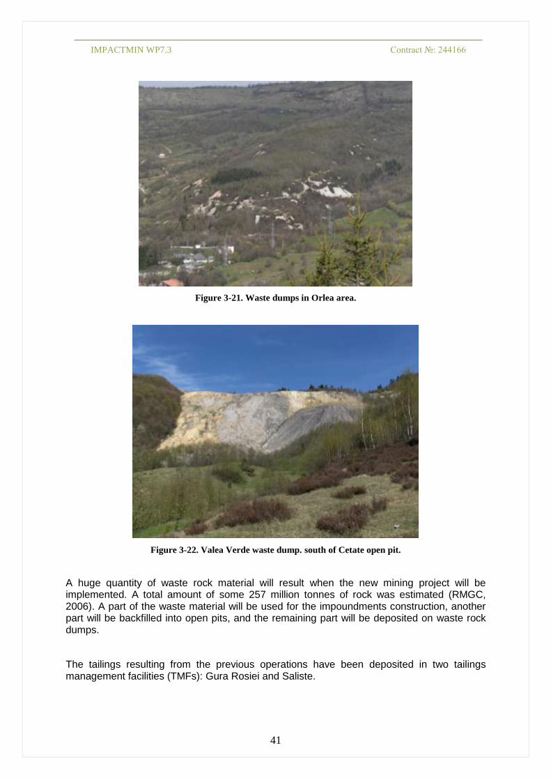
IMPACTMIN WP7.3 Contract №: 244166
41
Figure 3-21. Waste dumps in Orlea area.
Figure 3-22. Valea Verde waste dump. south of Cetate open pit.
A huge quantity of waste rock material will result when the new mining project will be implemented. A total amount of some 257 million tonnes of rock was estimated (RMGC, 2006). A part of the waste material will be used for the impoundments construction, another part will be backfilled into open pits, and the remaining part will be deposited on waste rock dumps.
The tailings resulting from the previous operations have been deposited in two tailings management facilities (TMFs): Gura Rosiei and Saliste.

IMPACTMIN WP7.3 Contract №: 244166
42
Recently, Gura Rosiei TMF has been rehabilitated, by being covered with a geomembrane and a soil layer, which is currently supporting herbaceous vegetation (
Figure 3-23). Consequently, it is not accessible for sampling or other investigations. The
rehabilitation process on Saliste TMF is still in progress, and its completion is planned for 2013.

IMPACTMIN WP7.3 Contract №: 244166
43
Figure 3-23. Gura Rosiei tailings pond (a) before reclamation and (b) during the reclamation works.
The RMGC mining project proposes a very large new TMF on Corna Valley. The dam of the TMF will be gradually raised up to the final height of 180 m. The total volume of tailings to be contained by the TMF is 172 M m3.
A test was performed in order to predict the behaviour of the tailings after the TMF will be operational. Different amounts of rock from Carnic and Cetate pits have been mixed, trying to simulate the conditions occurring at different steps of the mining project:
Sample RM1 – Dacite dominated with 80% from Cârnic and 20% from Cetate, Sample RM2 – Dacite and mixed breccia with 33% from Cârnic and 67%; Sample RM3A – Dacite dominated with 100% percent from Cârnic. The abundances of the minerals expected to occur in the tailings are listed in table NN.
a
b

IMPACTMIN WP7.3 Contract №: 244166
44
Table 3-4. Mineral abundances in talings material (RMGC, 2006)
Minerals Abundance (wt%)
Apatite 0 – 0.20
Chalcopyrite 0 – 0.05
FeMn-carbonate 0 – 1.30
Galena 0 – 0.12
Muscovite 10.90 – 13.00%
Orthoclase 59.10 – 67.20
Pyrite 2.30 – 5.10
Quartz 17.50 – 22.40
Rutile 0.13 – 0.38
Sphalerite 0 – 0.08
The main minerals that have been identified are potassium feldspar, quartz, and mica. The relatively high amount of pyrite, up to 5.10%, could potentially give acid drainage when the oxidative conditions are met.
The acid rock drainage potential has also been investigated by a field-based kinetic test that was started in August 2003, and it’s still running (MWH, 2005; RMGC, 2006, Costin et al, 2011). Different procedures were used to characterize the ARD potential of the waste rock from the Project area. The Acid-Base Accounting (ABA) method was applied in the initial stage, in order to evaluate the quantities of acid generating and acid-neutralising materials hosted by the waste rock. Additionally, the waste rock characterization program was completed by three forms of kinetic testing: Synthetic Precipitation Leaching Procedure, laboratory column testing, and field column testing (RMGC 2006). Several types of waste rock were separated, mainly: dacite, vent breccia, black breccia, andesite, and Cretaceous sedimentary rocks. The first three types are subsequently classified by silicified/potassic alteration type (abbreviated as SIK), and non-silicified/non-potassic (NSIK), which is generally argillic but may include unaltered rock or other less intense alteration types (like propylitic).
The test was conducted on 26 plastic barrels filled with rock samples, weighing about 300 kg each (Figure 3-24, Figure 3-25). The rock samples are exposed to the atmospheric conditions.
The leachate produced in each barrel is sampled periodically through a sampling port at the base of the barrel and analysed in the laboratory. The acid drainage was observed in 9 out of the 26 barrels (approximately 35% of the total). The vent and black breccia samples proved to yield more acidic waters compared to dacite.

IMPACTMIN WP7.3 Contract №: 244166
45
Figure 3-24. The acid drainage test site.
Figure 3-25. Plastic barrels with rock samples used for the kinetic test.

IMPACTMIN WP7.3 Contract №: 244166
46
4 Chemical characteristics of soil and vegetation
4.1 Sample collection, preservation, and handling
4.1.1 Soils sampling strategy Soils occur in a wide variety of settings and geomorphological contexts, and for the purpose of remote sensing interpretation we have subdivided the soils in different classes according to where they occur:
1) Soils on or near the deposits (Figure 4-1a, b). These are mostly red-yellow-brown
coloured soils that are formed as a result of weathering of the altered rocks. Their
extent is limited to at most a few hundred meters away from the deposits. Vegetation
on these soils is usually poor and shrubby
2) Soils in scarps (Figure 4-1c), landslides, road-cuts, etc. These locations often form
sharp contrasting transitions in the landscape. They are often poorly vegetated
because the lack of water and continuing erosion
3) Soils in grasslands (Figure 4-1d-i). These clayish soils have all kinds of shades from
brown to grey, to cream-coloured, and can be in situ as well as colluvial. Colours vary
from brownish to whitish.
Soil samples were collected in three different campaigns (Figure 4-2).
During the 2011 campaign we focused on soils in direct vicinity of the known deposits (Figure
4-1a, b). Samples were measured with the ASD spectrometer and analysed for a number of trace elements: Cu, Pb, Zn, Ni, Cr, Cd. In the same campaign, a limited number of stream sediment samples from streams around the deposit have been collected. They were analysed similarly to the soil samples.

IMPACTMIN WP7.3 Contract №: 244166
47
Figure 4-1. Different categories of soil exposures. Soils in the mineralized areas (a, b), in scarps, road cuts
etc (c), in uncut grasslands (d), in recently cut grassland (e), in grazing lands with molehills (f), in grazing
land with decreasing vegetation density (g-i).
The May 2012 campaign focused on regional soils in grasslands. Soil samples were collected on predefined traverses in grasslands for spectral and chemical analysis.
The planning of the traverses was based on the following:
- The variations we observed for the grasslands in the 2010 and 2011 Worldview2
imagery (see Figure 5-10). We tried to cover different types of grasslands with different
density of vegetation
- Distance to the known mineralized areas. We tried to collect representative samples
in different directions, and different distances in order to identify the spatial extent of
current mineralization-related changes in soil mineralogy and composition.
- Geomorphologic variations: we tried to identify mineralogical changes resulting from
different geomorphologic environments such as slopes, hill-tops, valleys, etc.
- Statistical soundness: Soil characteristics can change within a small area, depending
on factors such as geomorphology, land use, ground water conditions, etc. Therefore
it is important that more than one sample is collected from each identified location, in
order to be able to assess the spatial variability within each specific location. This is
the reason why we collected samples on sections through each identified location.
During the July-2012 soil sampling campaign we focused in the first place on in-fill sampling covering the transition zone between the altered areas and the regional unaltered areas

IMPACTMIN WP7.3 Contract №: 244166
48
sampled in May. Secondly, a number of in-fill samples were taken to complement the May-2012 program, and a few additional regional samples were taken for comparison with the samples taken earlier that year. During the July-campaign we exclusively took samples from exposed soil, in contrast to the May-campaign, where soil samples were also taken from just below the grass-cover in cases where no soil was exposed. The samples collected during this campaign were used for spectral analysis only.
Figure 4-2. Location of soil samples taken during the respective field campaigns for spectral analysis with
contact probe.
4.1.2 Soil and sediment samples collection and processing The soil and sediments samples were collected from both mining and adjacent areas. The
sampling points were marked by GPS readings. The samples consisted of 150 – 500 g of
soil/sediment collected from surface layer (0 – 10 cm depth), using a clean stainless steel
shovel. The samples were put into polyethylene bags, well-sealed, and then were
transported to the laboratory where they were dried in open air, at ambient temperature, for
two weeks (US-EPA 3050B, ISO 11464). The roots and other mineral and organic material,
with a diameter larger than 2 mm, were removed by sieving (ISO 11464). The samples were
then dried in oven (Memmert UNB 400, Germany) at 105°C for 24 hours. In order to have a
homogeneous sample and to increase the efficiency of acid attack by increasing the surface
area of the particles, the samples were ground, using a mortar, to a size less than 150 µm
(ISO 11464). An amount of 100 g of ground soil/sediment was sieved using a 150 µm sieve
(Figure 4-3).

IMPACTMIN WP7.3 Contract №: 244166
49
Figure 4-3. Soils/sediments samples processed for digestion.
4.1.3 Leaves A total of 144 leaves samples were collected in two different campaigns in 2012 (June-July
2012 and August 2012). Leaves of Betula pendula and Carpinus betulus were collected from
different points of the study area: near to the open pit and tailings areas, near and on the
waste dumps or far away from the mining site. The strategy of the sampling methodology
was made in order to cover the entire mining area, including polluted and non-polluted
zones. These tree species are predominant in the area of interest of the project. The tree
species have been identified by biologists in the field and sampling points were marked by
GPS readings.
Leaves samples were collected for laboratory analysis pursuing the following parameters:
chlorophyll content, fluorescence and heavy metal content. Leaves from the bottom, middle
and top of the canopy plus leaves from one branch, were sampled and stored in a cooler box
for a good preserving before reaching the laboratory.
In the laboratory, the vegetation samples were dried in open air, at ambient temperature for
one month (Steinborn and Breen 1999). After drying, the samples were transferred in paper
bags well sealed until subsequent laboratory analyses. The samples were then dried in oven
(Memmert UNB 400, Germany) at 105°C for 24 hours Figure 4-3. Vegetation samples (0.5 – 5
g) were ground and homogenized in a blender before weighing aliquots for total heavy metal
content. The powdered samples were stored in clean polyethylene bags until analysis (within
7 days).

IMPACTMIN WP7.3 Contract №: 244166
50
4.2 Sample analysis
4.2.1 Measurement of the soil pH
The pH of the soils was potentiometrically measured in the supernatant suspension of a soil :
distilled water mixture (1 : 5) (ISO 10390).
Representative samples of 25 g were taken of the air-dried soil (fraction < 2 mm). Each
sample was placed in an Erlenmeyer flask and 125 ml of ultrapure water was added. The
mixture was shaken for 2 h; then, the mixtures were left for 30 min for the supernatant to
clearly separate Figure 4-4. The supernatant was then filtered and the pH was measured.
The pH was measured using a portable multiparameter WTW Multi 350i (Germany) Figure
4-5. Before the measurements, the multiparameter instrument was calibrated as prescribed
in the manufacturer’s manual, using the buffer solutions.
Figure 4-4. The pH measurement in soil/sediment samples.
Figure 4-5. Multiparameter device used for pH measurements.
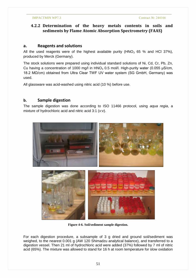
IMPACTMIN WP7.3 Contract №: 244166
51
4.2.2 Determination of the heavy metals contents in soils and sediments by Flame Atomic Absorption Spectrometry (FAAS)
a. Reagents and solutions All the used reagents were of the highest available purity (HNO3 65 % and HCl 37%),
produced by Merck (Germany).
The stock solutions were prepared using individual standard solutions of Ni, Cd, Cr, Pb, Zn,
Cu having a concentration of 1000 mg/l in HNO3 0.5 mol/l. High-purity water (0.055 µS/cm,
18.2 MΩ/cm) obtained from Ultra Clear TWF UV water system (SG GmbH, Germany) was
used.
All glassware was acid-washed using nitric acid (10 %) before use.
b. Sample digestion
The sample digestion was done according to ISO 11466 protocol, using aqua regia, a
mixture of hydrochloric acid and nitric acid 3:1 (v:v).
Figure 4-6. Soil/sediment sample digestion.
For each digestion procedure, a subsample of 3 g dried and ground soil/sediment was weighed, to the nearest 0.001 g (AW 120 Shimadzu analytical balance), and transferred to a digestion vessel. Then 21 ml of hydrochloric acid were added (37%) followed by 7 ml of nitric acid (65%). The mixture was allowed to stand for 16 h at room temperature for slow oxidation

IMPACTMIN WP7.3 Contract №: 244166
52
of the organic matter from the soil/sediment. The temperature of the reaction mixture was raised slowly until the reflux conditions were reached and then it was maintained for 2 h Figure 4-6. The digested samples were then filtered and the filtrate was collected in a 100 ml volumetric flask and brought to volume (100 ml) with HNO3 0.5%. The clear supernatant was analysed by FAAS. For each set of measures, one blank was prepared using the same procedure.
The digestion was carried out in a well-ventilated fume hood.
c. FAAS system All the determinations were performed by a ZEEnit 700 atomic absorption spectrometer
Figure 4-7 using an acetylene–air (C2H2-air) flame and the adequate cathode lamps at the
recommended current and conditions, specified in the FAAS Operators’ Manual. The
operating conditions for the FAAS are presented in Table 4-1.
Figure 4-7. FAAS system.
Table 4-1. The operating conditions for the FAAS.
Heavy metal Cr Cd Ni Zn Pb Cu
wavelength (nm) 357.9 228.8 232.0 213.9 283.3 324.8
HCL* current (mA) 5 3 5 4 3 3
slit width (nm) 0.2 1.2 0.2 0.5 1.2 1.2
flame C2H2/air C2H2/air C2H2/air C2H2/air C2H2/air C2H2/air
fuel flow (N l/h) 100 50 55 50 65 50
C/O stoichiometric 0.25 0.075 0.12 0.075 0.13 0.075
*HCL – Hollow-Cathode Lamps

IMPACTMIN WP7.3 Contract №: 244166
53
d. Analytical determination / quality control measures In order to ensure the quality of the data, the following parameters were studied: linearity, sensitivity and precision.
Linearity
The quantification analysis of the selected metals was done based on the external standard
method. The calibration linearity was investigated based on five/seven concentrations,
depending on the metal. The standard solutions were prepared by serial dilutions with HNO3
(0.5%) of the stock solution (50 mg/l). Each calibration standard was injected three times.
The correlation coefficients (R2) were also calculated. The calibration curves are presented in
Figure 4-8.
Figure 4-8. Calibration curves of the investigated metals.
The analyses demonstrated that the FAAS method had a good linearity since the correlation
coefficients were over 0.99 on the whole range of concentrations.
Sensitivity
The sensitivity of the FAAS method was estimated as the limit of detection (LOD) and the
limit of quantification (LOQ). The LOD and LOQ were calculated according to the IUPAC
(International Union of Pure and Applied Chemistry) rules on the basis of the standard

IMPACTMIN WP7.3 Contract №: 244166
54
deviation of the response and the slope, using the following equations (Thomsen et al. 2003,
Chan 2008, Sun and Li 2011).
SLOD
3 ;
SLOQ
10
where, “σ” is the standard deviation of 10 replicate measurements of the blank signal and “S”
is the slope of the calibration curve.
The FAAS method had a good sensitivity, with a LOD value between 0.012 and 0.083 mg/l
and a LOQ value between 0.039 and 0.276 mg/l, depending on the analysed metal (Table
4-2).
Table 4-2. LOD and LOQ of the FAAS method.
Metal Cr Cd Ni Zn Pb Cu
Linear working
range (mg/l)
0 – 1 0 – 1 0 – 1 0 – 1 0 – 1.5 0 – 3
LOD (mg/l) 0.035 0.012 0.038 0.013 0.083 0.036
LOQ (mg/l) 0.118 0.039 0.126 0.042 0.276 0.119
LOD (mg/kg) 1.167 0.400 1.266 0.420 2.767 1.187
LOQ (mg/kg) 3.933 1.300 3.769 1.407 9.213 3.966
For some samples, where the metals level was lower than the LOD, the samples were
spiked with a known concentration of standard solution in order to increase the LOD level.
Precision
The intermediate precision (defined as the variation within the same laboratory) of the quantitative determination of heavy metals was determined by the evaluation of repeatability (intra-day precision) and of the intermediate precision (inter-day precision) (Chan, 2008). For both intra- and inter-day study, five replicates of heavy metals standard solutions were analyzed and the RSD values were calculated Table 4-3.
Table 4-3. Intra-day and inter-day precision of the FAAS method.
Metals Conc. (mg/l)
Intra-Day Precision Inter-Day Precision
Measured Conc.
(mg/l) Mean SD*
RSD** [%]
Measured Conc.
(mg/l) Mean SD
RSD [%]
Cr 0.25 0.251 0.016 6.37 0.247 0.013 5.26
Cd 0.05 0.054 0.003 6.52 0.048 0.003 6.25
Ni 0. 5 0.513 0.028 5.52 0.488 0.025 5.12
Zn 0.5 0.510 0.016 3.11 0.514 0.021 4.08
Pb 0.5 0.5050.029 5.81 0.499 0.027 5.47
Cu 1.5 1.55 0.04 2.50 1.52 0.04 3.53 *SD- Standard Deviation
, ** RSD-Relative Standard Deviation

IMPACTMIN WP7.3 Contract №: 244166
55
As shown in Table 4-3, the RSD for the intra-day precision ranged between 2.50 and 6.52%,
while the RSD for the inter-day precision was between 3.53 and 6.25%. The results of the
analyses show that the FAAS method has a good precision demonstrated by the low RSD
obtained for both intra- and inter-day repeatability.
e. Calculations
The method blank contained detectable concentrations of metals and these concentrations
were subtracted from the sample concentration. In order to report the metal concentration as
mg/kg in dried soil or sediment, the metal concentration from the soil extract was multiplied
by the dilution and divided by the mass of dried soil/sediment. The following formula was
used:
)(
)(100(mg/l)extract in ion concentrat metal (mg/kg) soilin ion concentrat metal
gmasssoil
ml
4.2.3 Determination of heavy metals in vegetation by Inductively Coupled Plasma – Mass Spectrometry (ICP-MS)
Figure 4-9. Vegetation samples processed for digestion.
a. Reagents and solutions All reagents used were of the highest available purity (HNO3 65 %), produced by Merck
(Germany). For this study, NIST 2709 and NIST 1643e certified reference materials were
used to check the accuracy of the method. High-purity water (0.055 µS/cm, 18.2 MΩ/cm)
obtained from Ultra Clear TWF UV water system (SG GmbH, Germany) was used.
All glassware was acid-washed using nitric acid (10 %) before use.

IMPACTMIN WP7.3 Contract №: 244166
56
b. Sample digestion
The leaves digestion was done using a Mars 5 microwave digestion system (CEM, USA) (Figure 4-9, Figure 4-10).
Figure 4-10. Samples digestion (left: during digestion; right: after digestion).
For the digestion procedure, around 1g subsample of dried and ground vegetation was
weighed, to the nearest 0.001 g (AW 120 Shimadzu analytical balance), and transferred to a
digestion vessel. A quantity of 5 ml of nitric acid (65%) was added, and the vessels were
shacked for several minutes and after 10 min of waiting, the vessels were closed and placed
in the rotor of the Mars microwave digestion system. The adequate digestion program was
optimized according to the instructions specified in the microwave Operators’ Manual, and
consisted in heating the samples in two steps: (1) increase the power by 80% (300 W) for 10
min and (2) decrease the power by 55% for 10 min.
After cooling, the digested samples were filtered and subsequently diluted to 25 ml with
ultrapure water and the clear supernatant was analyzed by ICP-MS. For each set of
measures, one blank was prepared using the same procedure.
c. The ICP-MS system The investigated elements (Ag, Al, As, Au, B, Ba, Be, Bi, Br, Ca, Cd, Ce, Co, Cr, Cs, Cu, Dy,
Er, Eu, Fe, Ga, Gd, Ge, Hf, Hg, Ho, I, In, Ir, K, La, Li, Lu, Mg, Mn, Mo, Na, Nb, Nd, Ni, Os,
Pb, Pd, Pt, Rb, Pr, Re, Rh, Ru, Sb, Sc, Sm, Sn, Sr, Ta, Tb, Te, Th, Ti, Tl, Tm, U, V, W, Y,
Yb, Zn, Zr) were analyzed by the application of mass spectrometry with inductively coupled
plasma (ICP-MS). For ICP-MS measurements a SCIEX Perkin Elmer Elan DRC II (Canada)
inductively coupled plasma mass spectrometer (with quadruple and single detector setup)
was used Figure 4-11. The instrumentation and operating conditions for the ICP-MS system
are presented in Table 4-4.

IMPACTMIN WP7.3 Contract №: 244166
57
Figure 4-11. ICP-MS system.
Table 4-4. Instrumentation and operating conditions for the ICPMS system [Baceva et al. 2012].
Parameter Value
Plasma
Power
Plasma gas flow
Auxiliary gas flow
Nebuliser gas flow
Sample/Skimmer cone
1350 W
12.00 l/min
1.20 l/min
1.05 l/min
Platinum
Quadrupole
Quadruple rod offset (QRO)
Cell rod offset (CRO)
Cell path voltage (CPV)
Measurement mode
Dwell time/ms
Integration time/ms
Reading per point
Reading per replicate
Replicate measurements
V
−8.00 V
−20.00 V
Peak hopping
Varying
Varying
300
1
4
DRC
Reaction Gas
Lens voltage
None
11.00 V
The dynamic reaction chamber (DRC) was used in RF only mode (no gas) and its parameters were previously optimized (Tanaselia et al., 2008). For the sample introduction system, a classic setup was used consisting of a peristaltic pump, a Meinhard nebuliser and a cyclonic spray chamber, where fine aerosols are formed, that go directly into the plasma (Baceva et al., 2012).

IMPACTMIN WP7.3 Contract №: 244166
58
d. Analytical determination / quality control measures All measurements were conducted using the semi-quantitative method (TotalQuant) supplied
by the Elan 3.4 software that uses a response factor calibration curve which was obtained by
calibration at multiple points (low, medium and high mass for optimum set-up), using a
multielement Merck VI standard solution, diluted to mimic real sample composition (Baceva
et al., 2012).
In order to check the accuracy of the method, a NIST 2709 and NIST 1643e certified
reference materials were used. For all the investigated elements, the difference between the
measured and certified values was within 15% (Baceva et al., 2012).
The theoretical limit for ICP-MS methods are in the ppt (ng/l) range for the majority of the
elements. By using TotalQuant method, no matrix effects were observed for concentrations
above 1 ppb (1 μg/l) (Baceva et al., 2012).
Quality control was also ensured by standard moss reference materials M2 and M3, which
are prepared for the European Moss Survey (Steinnes et al., 1997). The measured
concentrations were in good agreement with the recommended values.
The method of standard additions was also applied and quantitative recoveries were
achieved for the most of the elements (Baceva et al., 2012).
e. Calculations
The method blank contained detectable concentrations of metals and these concentrations
were subtracted from the sample concentration. In order to report the metal concentration as
mg/kg in dried vegetation, the metal concentration from the sample was multiplied by the
dilution and divided by the mass of dried vegetation which was multiplied by 1000. The
following formula was used:
1000)(
)(25g/l)(extract in ion concentrat metal (mg/kg)ion in vegetation concentrat metal
gmassvegetation
ml
4.2.4 Determination of chlorophyll content and fluorescence in leaves
a. Measurement procedure for leaves
The sampling methodology is the same as in the case of heavy metals determination in
leaves.
The measurement procedure for chlorophyll content in leaves is presented in Table 1. After
chlorophyll determination, the same leaves samples were used for fluorescence
determination.
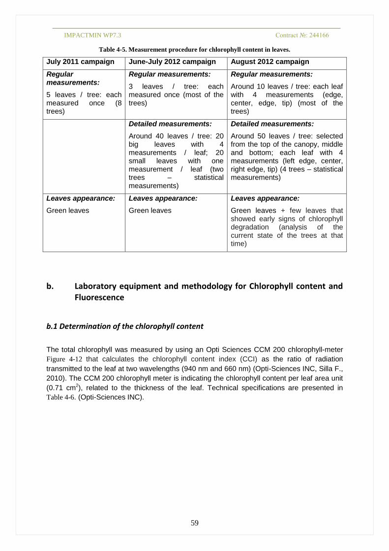
IMPACTMIN WP7.3 Contract №: 244166
59
Table 4-5. Measurement procedure for chlorophyll content in leaves.
July 2011 campaign June-July 2012 campaign August 2012 campaign
Regular measurements:
5 leaves / tree: each measured once (8 trees)
Regular measurements:
3 leaves / tree: each measured once (most of the trees)
Regular measurements:
Around 10 leaves / tree: each leaf with 4 measurements (edge, center, edge, tip) (most of the trees)
Detailed measurements:
Around 40 leaves / tree: 20 big leaves with 4 measurements / leaf; 20 small leaves with one measurement / leaf (two trees – statistical measurements)
Detailed measurements:
Around 50 leaves / tree: selected from the top of the canopy, middle and bottom; each leaf with 4 measurements (left edge, center, right edge, tip) (4 trees – statistical measurements)
Leaves appearance:
Green leaves
Leaves appearance:
Green leaves
Leaves appearance:
Green leaves + few leaves that showed early signs of chlorophyll degradation (analysis of the current state of the trees at that time)
b. Laboratory equipment and methodology for Chlorophyll content and Fluorescence
b.1 Determination of the chlorophyll content
The total chlorophyll was measured by using an Opti Sciences CCM 200 chlorophyll-meter
Figure 4-12 that calculates the chlorophyll content index (CCI) as the ratio of radiation
transmitted to the leaf at two wavelengths (940 nm and 660 nm) (Opti-Sciences INC, Silla F.,
2010). The CCM 200 chlorophyll meter is indicating the chlorophyll content per leaf area unit
(0.71 cm2), related to the thickness of the leaf. Technical specifications are presented in
Table 4-6. (Opti-Sciences INC).

IMPACTMIN WP7.3 Contract №: 244166
60
Figure 4-12. Opti Sciences CCM 200 chlorophyll-meter.
Table 4-6. Technical Specifications CCM-200 Chlorophyll Content Meter (Opti-Sciences INC).
Measurement technique Optical absorbance in two wavebands
Measured area 1cm diameter circle
Accuracy +/- 1 CCI unit
Sample acquisition time 2-3 seconds
Source Two LEDs
Detectors Two temperature compensated silicon photodiodes
Storage 4,000 data sets
User interface 16 x 2 alphanumeric LCD
Output RS-232 with supplied PC software
Operating temperature range 0 – 50°C
Battery 4AA cells
Weight 180g (excludes battery)
Dimensions 150 82 x 25mm
b.2 Preparing the leaves samples for pigments extraction
An amount of 0.5 – 2 g of each leaves samples was weighed Figure 4-13 and transferred to a
glass vessel, and 25 ml 95 % ethanol were added. Pigments were extracted Figure 4-14 by
boiling the samples for 10 min at 80°C using the FALC Heating Mantles without stirring (Fig
3). The boiling process is continued until the absolute discoloration of the leaves is achieved.
The extracts were cooled and collected in a 50 ml brown volumetric flask and brought to
volume with 95% ethanol.

IMPACTMIN WP7.3 Contract №: 244166
61
Figure 4-13. Leaf samples prepared for analysis
Figure 4-14. The process of heating and separation using FALC Heating Mantles.
b.3 Determination of Photosynthetic Pigment concentrations
The absorbance of crude extracts was measured on a Metertek SP-850 spectrophotometer
(Metertech-inc, Taiwan) Figure 4-15 at the following wavelengths: 665 nm for chlorophyll a;
649 nm for chlorophyll b; 470 nm for carotenoids. If the pigment extract is too concentrated,
dilutions are made with 95 % ethanol. After each reading, the spectrophotometer is
calibrated with 95 % ethanol.
Technical Specifications for Metertek SP-850 (Metertech-inc, Taiwan) are presented in Table
4-7.

IMPACTMIN WP7.3 Contract №: 244166
62
Figure 4-15. Metertek SP-850 spectrophotometer
Table 4-7. Technical Specifications for Metertek SP-850 spectrophotometer (Metertech-inc, Taiwan)
Model SP-850
MONOCHROMATOR Diffraction grating
WARM-UP TIME, min (WAVELENGTH, nm) 20
PATH LENGTH, mm (WAVELENGTH, nm) 10
Linearity (WAVELENGTH, nm) 0.01
Precision (WAVELENGTH, nm) 1% @ 1 A
Reproducibility (WAVELENGTH, nm) <1%
ZERO DRIFT (WAVELENGTH, nm) 0.003 A/hr
340 nm (SCATTERED LIGHT) <0.5%
DATA MANAGEMENT Absorbance, transmittance, concentration, factor
DISPLAY LED
POWER NEEDED 115/230, 50/60 Hz
LAMPS Tungsten
Duration, hr (POWER NEEDED) 1
Range (WAVELENGTH, nm) 330-999
Precision (WAVELENGTH, nm) 2
BANDPASS, nm (WAVELENGTH, nm) 8
Photosynthetic pigment concentrations were calculated by using established equations that estimate concentration as a function of absorbance of foliar extracts at specific wavelengths (Lichtenthaler, 1987, Zhuo Shen et al, 2009):
FWgmgDVWd
AA
/
1000
88.695.13a lChlorophyl 649665
FWgmgDVWd
AA
/
1000
32.796.24b lChlorophyl 665649

IMPACTMIN WP7.3 Contract №: 244166
63
FWgmgDVWd
clfclfA ba
/
1000245
8.11405.21000Carotenoid 470
where: A – absorbance at a certain wavelength, V – volume of total extract, D – coefficient of
dilution, FW – fresh weight (g), d = 1cm (internal width of cuvette), 1000 – µg to mg
conversion factor. When expressed on the basis of sample fresh weight, the correction factor
was the actual volume of the extraction divided by the sample fresh weight.
b.4 Fluorescence determination
An OPTI SCIENCES – OS1-FL modulated fluorometer (Opti-Sciences INC, OS1-FL
Brochure) Figure 4-16 was used for measuring the parameters of the chlorophyll
fluorescence. The following indices were determined: Fo – basal fluorescence, Fm – maximal
fluorescence, Ft – instantaneous fluorescence signal, Fv/Fm – maximum quantum efficiency
(Photochemical efficiency of PSII) and Fv – variable fluorescence which is calculated as
follows: Fv = Fm – Fo.
Technical Specifications for OS1-FL modulated fluorometer (Opti-Sciences INC, OS1-FL Brochure) are presented in Table 4-8.
Table 4-8. Technical Specifications for OS1-FL modulated fluorometer (Opti-Sciences INC, OS1-FL
Brochure)
Parameters Measured: Y, Fs, Fms, Fv/Fm, Fo, Fm
Detection method: Pulse modulation method
Detector & Filters: A PIN photodiode with a 700 ~750 nm bandpass filter
Saturation pulse 35 Watt halogen lamp with 690 nm short pass filter. 15,000uE
Modulated light 660 nm LED with 690 nm short pass filter.
Sampling Rate: Autoswitching from 10 to 10,000 points per second, depending on phase of test.
Test Duration: Adjustable from 2 seconds ~ 45minutes (optional 2 seconds ~ 16 hours.)
Storage Capacity: 128 Kb battery backed up RAM, supporting up to 4,000 test data sets, or 1trace up to 45 min.
Digital Output: RS-232 port
User Interface: Display: 20 x 4 Character super-twist LCD
Keyboard: 12 key dedicated function layout
Power Supply: Internal 12V, 1.2 Ah rechargeable sealed lead-acid battery.
Battery Life: Up to 6 hours of continuous operation
Dimensions: 7 cm x 11 cm x 19 cm.
Weight: 2 kg

IMPACTMIN WP7.3 Contract №: 244166
64
Figure 4-16. OPTI SCIENCES – OS1–FL fluorometer
4.3 Results of soils and sediments chemical analyses
During the field campaigns preformed in 2011 and 2012, more than 600 soils and sediments samples were collected from all over the study area Figure 4-17. All of them have been
hyperspectrally measured using a spectroradiometer, and subsequently, a selection of more than 200 samples representative samples have been analysed in the laboratory. The pH in water slurry, and the heavy metals contents (Cd, Cr, Cu, Ni, Pb, Zn) were determined, following the protocols described in chapter 4.
Figure 4-17. Soil sampling in Jig area.

IMPACTMIN WP7.3 Contract №: 244166
65
Figure 4-18. Spatial distribution of the soil pH values in the study area (left) and frequency (right).
According to the pH reference values (Ministerial Order 278/2011), most of the soils are acidic (strongly acidic – 63 samples, pH < 5.00; moderately acidic – 74 samples, pH=5.01-5.80; weakly acidic – 61 samples, pH=5.81-6.80) (Figure 4-18). Very few samples have
shown neutral (3 samples, pH=6.81-7.20) or weakly alkaline (3 samples, pH=7.21-7.67) reaction. Lower pH values, corresponding to strong acidic soils, may be observed in the mining area and in its proximity, including the open pits, galleries, and other objects generated by the mining activity, as waste rock dumps and tailings deposits. The sediments along the streams that receive water coming from the open pits, galleries, or percolating the waste rock piles and tailings, have a very pronounced acidic reaction. Figure 4-18 shows the
spatial distribution of the soil acidity in the project’s area. One may notice low pH areas in Cetate and Carnic open pits, on Saliste tailings management facility, and along the Rosia Valley, that is heavily polluted by the acid waters coming from underground works, as Adit 714, and some other galleries upstream of this. Acidic soils also occur in the proximity of the smaller mineralised areas that have been mined in the past, Orlea and Jig-Vaidoaia. In very few cases, an alkaline reaction has been detected. The acidity of soils and sediments reflects the intensity of the acid rock drainage/acid mine drainage (ARD/AMD).
The acid solutions facilitate the weathering of rocks, contributing to the mobilisation of the heavy metals, that could further concentrate in soils and sediments. The heavy metals contents in soils and stream sediments have been determined according to the methodology described in chapter 4.
The distribution in soils and stream sediments of the six heavy metals that were analysed is presented in Figure 4-19.

IMPACTMIN WP7.3 Contract №: 244166
66
a b
c d

IMPACTMIN WP7.3 Contract №: 244166
67
Figure 4-19. Concentrations of heavy metals in soils and stream sediments: (a) Cu concentrations; (b) Pb
concentrations; (c) Cd concentrations; (d) Zn concentrations; (e) Cr concentrations; (f) Ni concentrations.
The heavy metals contents in soils and stream sediments have been compared with the Romanian to the reference values of MAPPM Order 756/1997. This regulation is setting up the values considered as normal contents of these chemicals in soil and values representing alert and response thresholds for sensitive soil use. Accordingly, we have considered four classes of values for each metal: below the normal value, between the normal value and the alert threshold, between the alert threshold and the intervention threshold, and above the intervention threshold. Most of the returned analytical results are in the range of the normal values, with some variations. Copper, lead, cadmium and zinc concentrations are in the range of normal values, slightly increased in the case of Cu, Pb, Cd, but still below the alert threshold. Increased values can be observed in the proximity of the mining areas and along the streams with low pH water. On the TMF, the contents are also low, the Pb is a little bit more concentrated, but below the intervention threshold. The Ni and Cr do not show a direct relation with the deposit. Some higher contents of Ni are scattered in remote zones by respect to the mine. Chromium content is low in the whole study area. The frequency of the heavy metals contents for each metal is presented in the graphs in Figure 4-20.
e f

IMPACTMIN WP7.3 Contract №: 244166
68
Figure 4-20. Frequency of the heavy metals contents in soils and stream sediments samples.
4.4 Results of chemical analyses on leaves
The state of the vegetation has been assessed by spectral measurements on leaves, combined with in situ and laboratory measurements of the chlorophyll content, and heavy metals content, determined in the lab. The experimental procedures that have been followed are described in chapter 4. Leaves from two tree species, birch (Betula pendula) and hornbeam (Carpinus betulus), have been sampled. A third species, Fagus sylvatica was initially considered in the study, but it was eliminated later on, due to its uneven distribution in the field, and the difficulty to obtain a homogeneous coverage of the area. Hyperspectral measurements were performed in the field on series of leaves. The total chlorophyll content was measured in the field using the Opti Sciences CCM 200 chlorophyll-meter. The pigments were further on extracted in the laboratory. The contents of chlorophyll a and b, and carotenoids were determined on the Metertek SP-850 spectrophotometer.

IMPACTMIN WP7.3 Contract №: 244166
69
Maps of the distribution of the heavy metals contents in plants have been produced based on chemical analyses, for Cd, Cr, Cu, Ni, Pb, Zn
Figure 4-21).

IMPACTMIN WP7.3 Contract №: 244166
70
a
b
c d

IMPACTMIN WP7.3 Contract №: 244166
71
h g
f e

IMPACTMIN WP7.3 Contract №: 244166
72
Figure 4-21. Heavy metals contents in leaves: (a) Cr in birch leaves; (b) Cr in hornbeam leaves; (c) Cu in
birch leaves; (d) Cu in hornbeam leaves; (e) Ni in birch leaves; (f) Ni in hornbeam leaves; (g) Pb in birch
leaves; (h) Pb in hornbeam leaves; (i) Cd in birch leaves; (j) Cd in hornbeam leaves; (k) Zn in birch
leaves; (l) Zn in hornbeam leaves.
i
l k
j

IMPACTMIN WP7.3 Contract №: 244166
73
The uptake of heavy metals by plants depends very much on their availability in soil. The uptake was found to be relatively similar for the two species in the case of Cr, Cu, Ni, and Pb
(

IMPACTMIN WP7.3 Contract №: 244166
74
Figure 4-21 a-h). However, the birch has the obvious tendency to uptake more Cd and Zn (

IMPACTMIN WP7.3 Contract №: 244166
75
Figure 4-21 i, k) than the hornbeam (
Figure 4-21 j, l). The two elements have also a comparable geochemical behaviour.
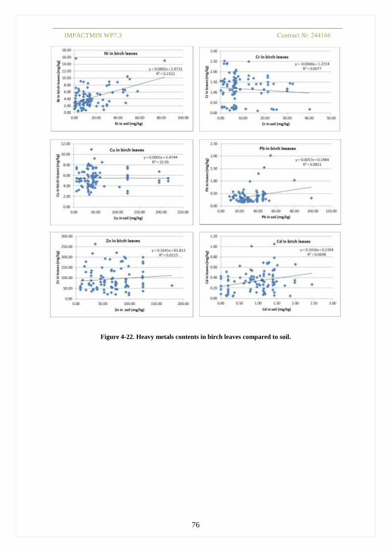
IMPACTMIN WP7.3 Contract №: 244166
76
Figure 4-22. Heavy metals contents in birch leaves compared to soil.

IMPACTMIN WP7.3 Contract №: 244166
77
Examining the concentrations of heavy metals in leaves and in soil in corresponding locations (
Figure 4-22), the low degree of correlation can be noticed for most of the metals. The tendencies are kept for the two tree-species, with slight positive correlation for Ni, Pb, and Cd, and negative tendency for Cr. The correlation degree for Zn and Cu is very low. According to the experimental data, seems that the birch has the ability to concentrate Zn up to 5 times by respect to the concentration in soil, in contrast with the hornbeam, where this tendency does not occur.

IMPACTMIN WP7.3 Contract №: 244166
78
Figure 4-23. Heavy metals contents in hornbeam leaves compared to soil.

IMPACTMIN WP7.3 Contract №: 244166
79
4.5 Results of the chlorophyll content and fluorescence measurements
The objective of this study was to examine the relationship between fluorescence emission spectrum and plant growth inhibition under stress conditions (in this case soil acidity and heavy metal contamination), and to investigate the degree of stress detectable from fluorescence measurements. Also destructive chlorophyll measurements were performed in order to establish a correlation between chlorophyll and fluorescence level. Changes in leaf pigment content and composition provide indications of tree stress
due to abiotic factors. The chlorophylls, Chl a and Chl b are essential pigments for the
conversion of light energy to stored chemical energy. The amount of solar radiation absorbed
by a leaf is a function of the photosynthetic pigment content (Monteith, 1972; Foyer et al.,
1982; Steele et al., 2008). Chlorophyll fluorescence is a measure of the efficiency of
photosynthesis and can be used, therefore, as an indicator of vegetation health and vitality
(Lichtenthaler et al., 1999; Kancheva et al., 2007).
The degree of stress was quantified through changes in leaf pigments because plant stressors affect the photosynthetic process causing a decline of the chlorophyll content. Fluorescence determination at leaf level is sensitive to chlorophyll content. This means that less chlorophyll concentration can lead to increasing fluorescence values (Kancheva et al., 2007). Very weak negative correlations r = -0.167 and r = -0.056 were established between soil pH and fluorescence parameter (Fv/Fm) in Betula pendula and in Carpinus betulus, meaning that the more acidic the soil is, the higher is the fluorescence. In the case of birch trees, there is a weak positive correlation of r = 0.139 between soil pH and total chlorophyll. As the soil reaction becomes less acid, the chlorophyll content is increasing. In the case of Carpinus betulus, the correlation becomes weak negative. All the chlorophyll content values and also the fluorescence values were plotted on a World View 2 image for better understanding the spatial distribution of the values (Figure
4-24).
The loss of chlorophyll and decline in photosynthesis are two of the phenomena associated with the process of stress in leaves of higher plants. Fluorescence can give a rapid and minimally invasive measurement of changes in a particular sample, giving insights into ability of the plant to tolerate environmental stresses and into the extent to which those stresses have damaged the photosynthetic apparatus.
Changes in Fv/Fm and Fo are accepted and widely used as reliable diagnostic indicators of photoinhibition. A decrease in Fv/Fm and an increase in Fo indicate the occurrence of photoinhibitory damage in response to stress.
Chlorophyll fluorescence can serve as sensitive indicators of heavy metals toxicity. As the concentration of heavy metal in soil is increasing, the fluorescence is also increasing, a positive linear relationship between heavy metal concentration and fluorescence being revealed. Low positive correlations were observed in case of Betula pendula and Carpinus betulus also, with one exception in case of Cr concentration in Betula pendula which presented a very weak negative correlation (r = -0.014).
Minor changes in Fv/Fm and Fo used as indicators of photoinhibition due to stress, have been determined. Furthermore, PSII photochemical efficiency, as determined from chlorophyll fluorescence, remained high, and the chlorophyll a/b ratio exhibited no decline except in leaves with extremely low chlorophyll contents.

IMPACTMIN WP7.3 Contract №: 244166
80
Figure 4-24. Chlorophyll content and fluorescence values in birch and hornbeam leaves.

IMPACTMIN WP7.3 Contract №: 244166
81
5 Hyperspectral measurements and remote sensing
5.1 Overview
From an environmental point of view, the area appears to be in a fairly steady state condition. The impact on the environment is inherited from former activities, and occurs in the form of open pits, waste dumps Figure 5-1, tailings dams Figure 5-2 and acid drainage originating from the open pits and underground galleries Figure 5-3.
Figure 5-1. Overview of the Rosia Montana deposit, showing the various open pits and waste dumps.
Figure 5-2. 3-D overview of the Saliste tailings dam, generated from Smartplanes aerial photography.
Since there are currently no mining-related processes that cause changes in the condition of the environment, we can regard the situation as relatively stable. This provides us with an excellent opportunity to create an environmental baseline for future mining activities using Remote Sensing technology. In order to establish an environmental baseline we have investigated the spectral variations and patterns that currently exist in all accessible categories of surface materials, such as drainages, rocks, soils and vegetation.
Detailed spectral laboratory analyses of drainage precipitates, soils and rocks in and around the historic and future mining areas (see Figure 5-4), soils and rocks outside of the direct sphere of influence of these mining areas, in-situ contact measurements of birch-leafs, in-situ

IMPACTMIN WP7.3 Contract №: 244166
82
solar reflectance measurements of soils and grasslands have been used, in combination with chemical analysis of the same materials, to characterize the current situation (Figure 5-5).
Figure 5-3. Acid drainage with Iron-rich chemical precipitate.
Multi-temporal Analysis of Worldview-2 imagery from three consecutive summers (2010, 2011 and 2012) has been used to assess the extent of normal variations in surface characteristics as a function of seasonal, climatic and normal land-use changes. The latter are mostly related to farming such as crop-rotation, irrigation, harvesting, forestry etc.
A low-altitude hyperspectral (VNIR) survey was carried out in summer 2012 giving us full hyperspectral coverage of the project area at 50 cm resolution.

IMPACTMIN WP7.3 Contract №: 244166
83
Figure 5-4. Proposed mining infrastructure showing the future open pits in green. Past mining areas are
located within the boundaries of the future open pits.
Figure 5-5. Locations of spectral samples from field campaigns 2011/2012. Red polygons indicate the
approximate outlines of the pits planned by RMGC, the yellow dashed line indicates the limit of the
Industrial Protection Area. A selection of the leaf and soil samples was used for chemical analysis.

IMPACTMIN WP7.3 Contract №: 244166
84
From a remote sensing point of view, the Rosia Montana district is a very complex and inhomogeneous area. The mountainous nature of the area results in a wide variety of geomorphological conditions, leading to typical alpine small-scale and diverse land-use, characterized by small parcels of grass land, separated by small forests and rows of trees. Farming land is primarily used for hay and grazing. Land-use patterns have probably not changed significantly over centuries, and most of the work is done in a very traditional manner (see Figure 5-6). Treed areas show a fairly high diversity of mostly deciduous
species, and locally with pine and fir trees.
Because of this complexity and high degree of spatial variability it was concluded that proper understanding of the Worldview2 and Hyperspectral imagery would improve significantly if we would have the availability of much higher spatial resolution data.
Although it was not foreseen in the original project scope, we therefore decided to acquire ultra-high-resolution aerial photography using the Smartplanes UAV, in order to be able to support the integrated interpretation of field data, hyperspectral imagery and Worldview2 imagery.
While the plan was to acquire Smartplanes imagery over significant portions of the project area, including the historic and future mining sites, this could not be realized because the permission for the flights was granted late. For that reason we decided to select two representative areas where we would fly the Smartplane, so that we at least could test our concept.
Figure 5-6. Traditional small-scale farming that is typical for this region. Cutting the grass is still done
manually using a scythe.
5.2 Field work
5.2.1 Field campaign 2011
During the 2011 field campaign our work focused primarily on the characterization of rocks, soils, streams and vegetation in the direct vicinity of the existing mining areas (Figure 5-7)
with the aim to understand the relationship between the mine in its current situation and various potentially related surface parameters (such as acid generation, vegetation stress, weathering and landslide-risk, anthropogenic disturbances, drought related to changes in the availability of ground water), and to establish criteria that will allow further mapping and

IMPACTMIN WP7.3 Contract №: 244166
85
monitoring of environmental impact of future mining activities using Remote Sensing imagery.
At the same time a hyperspectral survey was planned with the CASA 212 RS-INTA aircraft equipped with the AHS (VNIR-SWIR-TIR) sensor and the Casi1500i.
Due to bad weather conditions during the period that the hyperspectral over-flight and the vegetation measurements were planned, the airborne survey was cancelled and only a few vegetation measurements could be taken. This meant the loss of an excellent opportunity, taking into account the capabilities of the sensors mounted on the aircraft. At that time, a very important part of our dataset could not be acquired.
The interpretation of our 2011 field data, in combination with the analysis of the two Worldview2-images (acquired July 2010 and July 2011) demonstrated very clearly that the situation in Rosia Montana is much more complex than we had anticipated, and the environmental changes that can be anticipated to occur once the mine becomes active again are probably going to be of a very subtle nature even though they could become quite significant over periods longer than e.g. 20 years.
Figure 5-7. Locations of spectral samples from field campaign 2011. Red polygons indicate the
approximate outlines of the pits planned by RMGC, the yellow dashed line indicates the limit of the
Industrial Protection Area.

IMPACTMIN WP7.3 Contract №: 244166
86
Figure 5-8. Hyperspectral measurements of soil samples by the ASD spectrometer in the lab.
Figure 5-9. Hyperspectral measurements on leaves in the field
.
The results of the 2011 field campaign demonstrated that the most prominent variations in soil spectra are mostly related to underlying lithology. In most cases there was no direct correlation between the spectra of pure soils and the corresponding pixel spectra obtained from the Worldview-2 imagery (Figure 6-8), except for places where bare soil was clearly
exposed at surface. The reason for this lack of correlation can be found in the fact that in most cases soils are to some extent covered with grass, and even relatively small amounts of grass already mask the subtle spectral variations that are associated with the observed changes in soil composition.
Inspection of the WV2 imagery indicates that the grasslands show the most significant spectral variation, both within a single scene, and between imagery from consecutive years.
If we look at a natural colour composite (Figure 5-10a) we can see that there is a significant variation in greenness of the grasslands and that there appears to be a whole range of different types of grass land varying from almost bare soils to dense green grass lands.

IMPACTMIN WP7.3 Contract №: 244166
87
Figure 5-10. A) Natural colour composite of the 2010 WV2 image, illustrating the differences in greenness
of the grasslands. Arrows indicate examples of typical areas with different vegetation density. The image
corresponds with the yellow outline on the lower two images. B) Land classification of the WV2-2010
image. The colours of the classes correspond with the colours of the arrows. C) Land classification of the
WV-2011 image, using the same NDVI-thresholds as for the 2010 image.

IMPACTMIN WP7.3 Contract №: 244166
88
A rough first classification of the imagery using thresholded NDVI images shows the distribution of different classes of surfaces that progressively become greener (Figure 5-10b)
1) Bright surfaces, interpreted as Bare soils (Figure 5-10a, Red arrow)
2) Almost bare soils with some green or brown grass (Orange arrow)
3) Approximately equal proportions of soil and green/brown grass (Green arrow)
4) Mostly grass with some exposed soil (Blue arrow)
It should be noted that this is a fairly rough classification as its thresholds were defined in a subjective manner, and not based on any field calibration.
Nevertheless, comparison of the results for the images from 2010 and 2011 shows significant variations, and such a classification applied to multi-temporal imagery should be very suitable to identify systematic long-term changes in the vitality of the grasslands
These differences are probably the result of a highly complex interaction of natural and anthropogenic processes and parameters such as climatic variations, Land-use variations, biotic activity, soil fertility, groundwater regimes etcetera.
It is important however to be able to characterize these different types of grasslands because we expect that monitoring the long-term variations in the grasslands may be a very effective tool to identify systematic changes that are related to environmental impact from mining as opposed to naturally occurring variations.
While on the basis of our field observations we suspect that these differences can probably be explained by factors such as differences in water content of soils and grass, differences in length and density of grass, variations in proportion of exposed soil in grass lands, we concluded that we need more field observations in order to be able to explain more precisely the variations in the imagery.
The results from the 2011 field campaign also indicate that there are spectral differences between the leaf-spectra from birch trees located in vicinity of the open pit and those further away from the pit. This is illustrated in the plot of the red-edge position of the Birch trees (Figure 5-11), which is significantly lower for Birch trees located within boundaries of the
deposit. The red-edge position is a valuable parameter to assess the plant chlorophyll concentration and is often used as a vegetation stress index (Horler et al., 1983). A decrease in Red-edge position is usually related to increasing plant stress. For other species that were sampled, such as Pine trees, Beech, Acer and Poplar, we did not find any significant spatial variation in relation to the vicinity of the deposit. It must be noted though that Pine trees seem to have a preference for an acid environment, as they are abundant within the contours of the deposit, whereas they are relatively scarce beyond the limits of the deposit.

IMPACTMIN WP7.3 Contract №: 244166
89
Figure 5-11. Plot of Red-edge position for Birch leaves sampled in the 2011 field campaign. The spectral
plot shows some typical reflectance spectra for Birch leaves.
It became very clear that in order to be able to establish a proper environmental baseline, we needed to improve our understanding of the relation between (1) geological factors such as the presence of the deposit, lithology, geomorphology, (2) environmental factors, such as subtle changes in the mineralogical (e.g. clay, Iron-oxides) composition of soils, in the ground-water regime (e.g. drought), and in the health of vegetation (including grass-lands and trees), and (3) anthropogenic factors, such as land use dynamics, excavations, groundwater removal, aerial pollution, construction, increasing population, etc.
It also became clear that in order to be able to detect potential changes, we needed a stable reference, which meant that we had to collect our data at larger distances from the mining area, in areas that are not likely to be affected by future mining. Obviously, it is important that these “reference areas” are still within the same geologic, geomorphologic and climatic district.
Based on the results of the work we did in 2011 we concluded that it was necessary to plan an additional fieldwork campaign in 2012, which would focus on the following questions:
1) What is the normal relationship between geology and soil mineralogy, and what
happens to soils that are affected by mining activities? To this purpose we planned to
collect soil samples for laboratory spectral analysis.
2) Are there variations in vegetation stress that can be related to the vicinity of the
current mine and other known “unhealthy” environments such as the tailings dam,
dumps and the acid drainage? To this purpose we planned to investigate the variation
in plant stress indicators using foliage spectra from Birch trees.

IMPACTMIN WP7.3 Contract №: 244166
90
3) Is there a relation between plant stress and soil geochemistry? To this purpose we
planned to perform chemical analysis on soil and leaf samples.
4) Are soils and vegetation in affected areas more vulnerable and therefore more prone
to degradation and can we recognize the effects of increasing environmental impact
by looking at the quality of soils and at the vitality of grasslands and trees? To this
purpose we have taken spectra of soils, grasslands and tree foliage.
5) What is the meaning of the spectral variations we observe for grasslands in the WV2-
imagery? To this purpose we planned to document the appearance of grasslands in
detail, and to collect solar reflectance measurements of different types of grass-lands.
In order to be able to extrapolate the spot samples to the entire region of interest, it was decided that, in addition to collecting more data in the field, we would make another attempt to organize a hyperspectral campaign. However, since our budget was not sufficient to acquire both SWIR and VNIR, we had to decide which sensor would be most useful for our study.
As explained above, many of the questions that we encountered were related to vegetation, and we expect that potential environmental changes will in the first place have their impact on the vitality of vegetation – trees and grasslands. Since most of the spectral information related to vegetation is in the Visible and Near infrared region (350nm-1100nm) we decided that it was most effective if we acquire hyperspectral VNIR imagery. Since also the Worldview2-imagery has its information in the VNIR range, the hyperspectral imagery is expected to provide us a vital link in the interpretation chain of the Worldview2 imagery.
An innovative aspect of the planned hyperspectral survey is the fact that we would acquire data at 50 cm resolution. To achieve such a high resolution implies that the aircraft had to fly at altitudes of less than 750 m above ground. Given the rugged nature of the area, it was not only a challenge to fly the survey, but also to deal with consequences for the image geometry, inherent of the high vertical relief of the terrain.
We also found that many of the characteristic surface variations, in particular with respect to the strongly inhomogeneous nature of the grasslands and the treed areas, are at such a small scale that the resolution of the WV2 imagery and of the hyperspectral imagery is not sufficient to resolve important surface features (Figure 5-12). We simply do not see precisely
enough what we are looking at, which means that correct spectral interpretation and drawing the right conclusions is almost impossible, unless we have imagery that allows us to distinguish features such as individual trees, shrubs, small soil patches of exposed soil, freshly cut grass, hay, outcropping rock, etc.
For that reason we decided to bring the Smartplanes UAV to the field so that we could acquire ultra-high resolution imagery (4 cm resolution) for at least a part of the study area. Having such high-resolution imagery would very significantly enhance our ability to analyse the lower resolution hyperspectral imagery and the Worldview2 imagery.

IMPACTMIN WP7.3 Contract №: 244166
91
Figure 5-12. Comparison of Worldview2 Multispectral (2m resolution), WV2-pansharpened multispectral
(50 cm resolution), Hyperspectral VNIR (50 cm resolution) and Smartplanes image (4 cm resolution. The
red arrows point to the location of the soil exposure shown in the photograph. This type of soil exposure is
found frequently in grass lands used for grazing.
During the 2011 campaign, an experiment was conducted with the aim to develop an inexpensive, yet effective method to spectroscopically characterize a surface when hyperspectral imagery is unavailable. We have called this experiment the pseudo-hyperspectral evaluation. The goal was to identify the presence/source of acid-forming minerals in the mining-impacted areas. Two locations were chosen to setup the experiment: Saliste tailings dam, and Cetate open pit Figure 5-13, considered to be representative for the
impact of AMD in Rosia Montana area.
The samples were collected 10 m apart along two diagonal transects at the Saliste tailings dam and their location recorded with the GPS Figure 5-14 to Figure 5-16. About 250 grams of
loose sample was collected on each station and the samples were generally dry. The collected samples were powdery-to-fine in granularity and clayey in composition. In places, there were grey lenses of sulphide-rich sediments/layers about 2-3 cm in thickness. Similar collection procedure was repeated at the main pit (Cetate) of the former Rosia Montana open-pit mine, along the main East-West axis of the pit and, as possible, at each of the cut levels – pit bottom, intermediate haulage levels and pit top. The collected samples were comprised of about 30% hard rock samples, 30% gravel-sized chunks, 20% sandy samples (dry), 10% semi-moist muddy samples, and 10% dry-muddy samples. The majority of samples corresponded with the overall lithology expected for Rosia Montana: altered diatreme breccias with massive sulphides, altered dacites with presence of clay minerals, jarosite, chlorite and iron oxide staining.

IMPACTMIN WP7.3 Contract №: 244166
92
Figure 5-13. Location of Saliste tailings dam and Cetate pit.
Figure 5-14. Sample locations in the main pit of Rosia Montana Mine: Cetate
Figure 5-15. Sampling in Cetate Pit

IMPACTMIN WP7.3 Contract №: 244166
93
Figure 5-16. Sampling at Saliste tailings dam
5.2.2 Field campaign 2012
In summer 2012 three field campaigns were organized.
During the first campaign, which took place in May, more than 280 soil samples were collected for spectral and chemical analysis along 35 sections covering representative parts of the study area (see Figure 5-17).
During the second campaign (June 20 – July 5) the team has collected (see Figure 5-5):
55 additional soil samples for chemical and spectral analysis.
More than 400 solar reflectance measurements from soils, grasslands, rocks, open
pits.
Over 700 leaf spectra were measured from approximately 250 different Birch trees.
Leaf samples from 28 trees (hornbeam and birch) were collected for analysis of
chlorophyll and heavy metal content.
10 solar reflectance reference targets were measured for Empirical Line Correction of
the Worldview2 image, which was acquired while we were in the field, on July 4-2012,
Two Smartplanes UAV surveys covering approximately 0.5 km2 each.
The third campaign took place from Aug. 22 to Aug. 25, simultaneously with the hyperspectral overflight. The purpose of this field campaign was in the first place to collect reference material at the same time as the hyperspectral survey, and in the second place to gain some more specific insights related to the interpretation of the tree spectra. During the four days in the field the team collected leaves spectra and other samples as follows:
48 trees with on average 10 leaves per tree
4 trees with 50 leaves for in-depth statistical analysis
11 different tree species with focus on Betula and Carpinus
40 dried leaves
8 reference points for atmospheric validation

IMPACTMIN WP7.3 Contract №: 244166
94
Figure 5-17. Planned locations of sample profiles for the May-2012 field campaign (blue) and location of
the Smartplanes UAV survey blocks (red)
5.3 Preprocessing of WorldView 2 imagery
Worldview2 scenes were acquired in three consecutive years 2010, 2011 and 2012. All images were acquired between 7 and 11 July. The procedures for geometric and radiometric correction are described below:
Geometric correction:
All images were orthorectified using the Envi WV2-orthorectification tool. For the elevation model we used the 1m-resolution Orthophoto DEM made available by RMGC complemented by the 90m-resolution SRTM data. Obviously the great difference in spatial resolution is not very desirable, but we had no other choice, as the RMGC dataset covered only a part of our study area.
After the orthorectification there were small shifts between the three images. Those shifts were corrected by co-registering all images to the 2012 WV2 image. A number of precision ground control points provided by the RMGC-surveyor were used to position all scenes as accurately as possible.
Radiometric correction:
In order to be able to perform quantitative analysis of satellite imagery, to compare image spectra with field spectra, and to compare multi-temporal images, it is vital that all images are converted to absolute reflectance data. To do this, two steps are involved: (a) Radiance Correction (b) Atmospheric Correction.

IMPACTMIN WP7.3 Contract №: 244166
95
Radiance correction: DigitalGlobe’s WorldView image data is typically distributed in relative Radiance. We use the ENVI WorldView Radiance calibration utility to convert the relative
radiance into absolute radiance in units of
. This tool uses the calibration factors in
the WorldView-2 metadata file (the absCalFactor value in the .imd file) to perform the conversion.
Atmospheric correction: The solar radiation on the Sun surface-sensor ray path is subject to absorption and scattering by the atmosphere and the surface. Major atmospheric water bands centred at 0.94, 1.14, 1.38 and 1.88 micrometres, the oxygen band at 0.76 micrometre, and the carbon dioxide band near 20.8 micrometre are present. Approximately half of the 0.4-2.5 micrometre spectral region is affected by atmospheric gas absorptions. The shorter wavelength region below 1 micrometre is also affected by molecular and aerosol scattering.
Atmospheric correction attempts to minimize or remove the atmospheric influences that are added to the pure signal of the target and to extract more accurate information.
Accurate removal of atmospheric absorption and scattering effects is required in order to study surface processes using spectral imagery, and atmospheric correction is often considered critical pre-processing step to achieve full spectral information from every pixel especially with hyperspectral and multispectral data (Tyagi and Bhosle, 2011). This can be done using a variety of Atmospheric correction techniques (Gao et al., 2006).
In our study we have used the Empirical Line tool available in Envi. This method is an effective correction technique that provides an alternative to radiative transfer modelling approaches. The method uses ground spectra of ground reference targets to calibrate the imagery (Karpouzli and Malthus 2003). This method has been used successfully for Worldview-2 imagery (Staben et al. 2011). It is important that the ground reference spectra are measured as close to the moment of image acquisition as possible, in order to minimize the chance for differences in atmospheric conditions between the time of reference measurements and image acquisition.
For the field season 2011 we used a spectrometer equipped with a contact probe, whereas in 2012 we used a spectroradiometer, which allowed us to take solar reflectance measurements. As demonstrated further down in this report, the data obtained with contact probe measurements are not suitable for calibration of imagery. This has to do with the fact that a contact probe measures a very small surface (approx. 1cm2), while the Worldview2 pixel size is 2m. Given the heterogeneity of the land surface, it is almost impossible to obtain contact probe measurements that correspond exactly with the pixel spectra.
Our solar reflectance spectra from 2012 however covered a much larger surface. The measurements were taken with a bare fibre at approximately 120 cm above the ground. The bare fibre has a view angle of 21 degrees, which means that the area of view for a single measurement covers a circle with a radius of approximately 23 cm, which corresponds to a surface of 0.15 m2 This is still significantly less than the area covered by one pixel, but for relatively homogenous surfaces, such as asphalt roads, the tailings-dam surface, an artificial grass turf, a tiled roof, etc., we expect that the spectral measurement will be sufficiently similar to the satellite measurement to use as a reference for the 2012 WV2-image.
After empirical line correction we used the 2012 WV2 image as a reference for the atmospheric correction of the 2011 and 2010 images by calculating gain and offset factors from the scattergrams of the respective band-pairs. The resulting images show very acceptable correlation (see Figure 5-18).

IMPACTMIN WP7.3 Contract №: 244166
96
Figure 5-18. Scattergrams showing the relation (after atmospheric correction) of respectively bands 1,5
and 8 of WV2-2012 (horizontal axes) with WV2-2011 (vertical axes, figs a, b, c) and with WV2-2010
(vertical axes, figs d, e and f). The red lines indicate r=1.
A first step in analysing WV-2 images lies in filtering out trees or forests and agricultural fields based on a vegetation index combining bands 2 and 4 (Figure 5-19). In a second step, the forests were subdivided in different forest habitat types based on vegetation index values calculated from bands 5 and 7 (Figure 5-19c). The existing habitat map was subsequently
used as baseline to allocate habitat types and to conclude on the degree of pollution in the area. Based on this study, the green coloured areas in Figure 5-19d would most probably
indicate the presence of acidophilous beech trees, while the pink-white area represents beech and beech-oak forest. Finally, beech forests are shown in pink-red colours.
Also for grasslands and meadows, a further analysis was performed to describe the health status thereby focusing on leaf area index (LAI) of these habitats (Figure 5-19f). This was
possible by using an index combining bands 7 and 8.

IMPACTMIN WP7.3 Contract №: 244166
97
Figure 5-19. a. WordView-2 image, b. Habitat map, c. forest species highlighted on the habitat map, d.
classified WV2 map indicating different forest species, e. grasslands and meadows highlighted on the
habitat map, f. classified WV2 image of grasslands and meadows indicating different LAI values
a.
a
b
c d
f e

IMPACTMIN WP7.3 Contract №: 244166
98
5.4 Processing of Smartplanes imagery
Two areas were flown with the Smartplanes UAV (Figure 5-20). In order to obtain an image
resolution of 4-5 cm, we need to fly between 125-150 m above ground, whereas a survey altitude of 200 m AGL will give a photo resolution of approximately 7 cm. The areas that were flown are relatively steep, and show variations in terrain height of more than 200 m. This means that the surveys had to be planned very carefully in order to avoid serious terrain effects, such as blurred imagery, terrain distortions, inadequate overlap between flight-lines, strong variations in pixel size etc.
The aerial photographs from both surveys were processed to Orthophoto mosaics and Digital Terrain Models using Agisoft Photoscan software. When using precision ground control points, we are able to achieve a horizontal accuracy for the orthophotomosaic better than 7 cm, and a vertical accuracy of the DTM between 5 and 7 cm. If the ground control points are less accurate, the internal accuracy will remain, but the absolute accuracy will decrease accordingly.
In this case however, we had no precision ground control points, and we therefore decided to use a combination of ground control points that were measured with GPS, and ground control points taken from the WV2-imagery and the SRTM DEM. This implies that our absolute horizontal accuracy will be in the order of a few meters, whereas the absolute DTM accuracy will be at best similar to that of the SRTM DEM, which is somewhere between 4 and 16 m (Gorokhovic and Voustianiouk, 2006).
As a test, we have also performed a successful spectral analysis of the Smartplanes imagery demonstrating that the ordinary natural colour photography can be used for mapping Iron Oxides in soils and streams (see Figure 6-25, Figure 6-26).
5.5 Airborne hyperspectral survey
The hyperspectral survey was flown at an altitude of approximately 750 m above ground, resulting in imagery with approximately 50 cm resolution. To cover our area of interest (Figure
5-20), 19 lines were flown with a total line length of approximately 140 km. On 21, 22 and
23/08/2012 field measurements were taken with the ASD spectroradiometer to assess the quality of this imagery and to support the image analysis.

IMPACTMIN WP7.3 Contract №: 244166
99
Figure 5-20. Hyperspectral strips projected on the WV-2 natural colour image, showing the coverage
of the hyperspectral survey (red) and of the Smartplanes survey blocks (blue outlines).
On 20/08/2012 the AISA EAGLE system acquired the complete study area of Rosia Montana. In total 19 flightlines were flown by the HLB-SPECIM/Helsinki team, which details are found in Table 5-1.

IMPACTMIN WP7.3 Contract №: 244166
100
Table 5-1. Details of the hyperspectral flights acquired on 20/08/2012 above the Rosia Montana study area
On 21, 22 and 23/08/2012 field measurements were taken to assess the quality of the airborne imagery and form the basis for image analysis. Field measurements included:
ASD spectral reference measurements for dark and bright targets (Figure 5-21, Yellow
dots)
ASD spectral measurements of leaves, taken with the leaf clip (Figure 5-21, Red dots)
GPS measurements for georeferencing

IMPACTMIN WP7.3 Contract №: 244166
101
Figure 5-21. Location of spectral measurements of ground targets and leaves
5.6 Airborne data quality assessment
5.6.1 Quality of the geometric correction
Boresight calibration:
The boresight calibration was performed in Münster after mounting the scanner in the aircraft.
Geometric correction:
The data were geometrically corrected and orthorectified by the University of Helsinki, This was initially based on the use of the GPS/IMU flight data, and a detailed photogrammetric Digital Elevation Model supplied by RMGC. As the results showed significant errors (up to 10 m), it was decided to use the 2012 Worldview2-imagery to obtain more accurate ground control. This resulted in an accuracy of better than 1m for the central parts of the image strips. However, we found that there was a systematic increase in error towards the edges of the strip. This was investigated further, and could be explained by inaccurate correction of the focal length distortion. Since this effect was clearly visible when mosaicking the data, we decided to run an additional semi-automatic co-registration of each line with the 2012 Worldview2-image. This procedure reduced most of the geometric errors to less than 2 pixels
5.6.2 Quality of the radiometric correction The airborne data processing was executed by the University of Helsinki who delivered level-2, geometric and atmospheric corrected imagery. In a first phase two distinct atmospheric correction algorithms were tested, i.e. ATCOR 4 and FODIS. It was clear that ATCOR 4 performed better in removing atmospheric absorption features from the spectra, while some of these still remained after processing with FODIS (Figure 5-22).

IMPACTMIN WP7.3 Contract №: 244166
102
Figure 5-22. Comparison of the ATCOR vs FODIS atmospheric correction over an asphalt target.
In a next step, two distinct areas were selected from the EAGLE airborne dataset for ATCOR data processing and included bright (sand) and dark (asphalt) targets as indicated in Figure
5-23.
Figure 5-23. Ground reference targets identified in the AISA EAGLE dataset
The mean and standard deviation of these targets were calculated based on a 3*3 window around the target. The ASD measurements from the corresponding locations were processed and are given in Figure 5-24.

IMPACTMIN WP7.3 Contract №: 244166
103
Figure 5-24. Spectra of the ground reference targets measured with the ASD
The asphalt targets were already measured during a previous campaign (06/2012) with a Spectral Evolution spectrometer and could also be used additionally in the validation of the airborne data.
The results of the intercomparison are given in Figure 5-25.
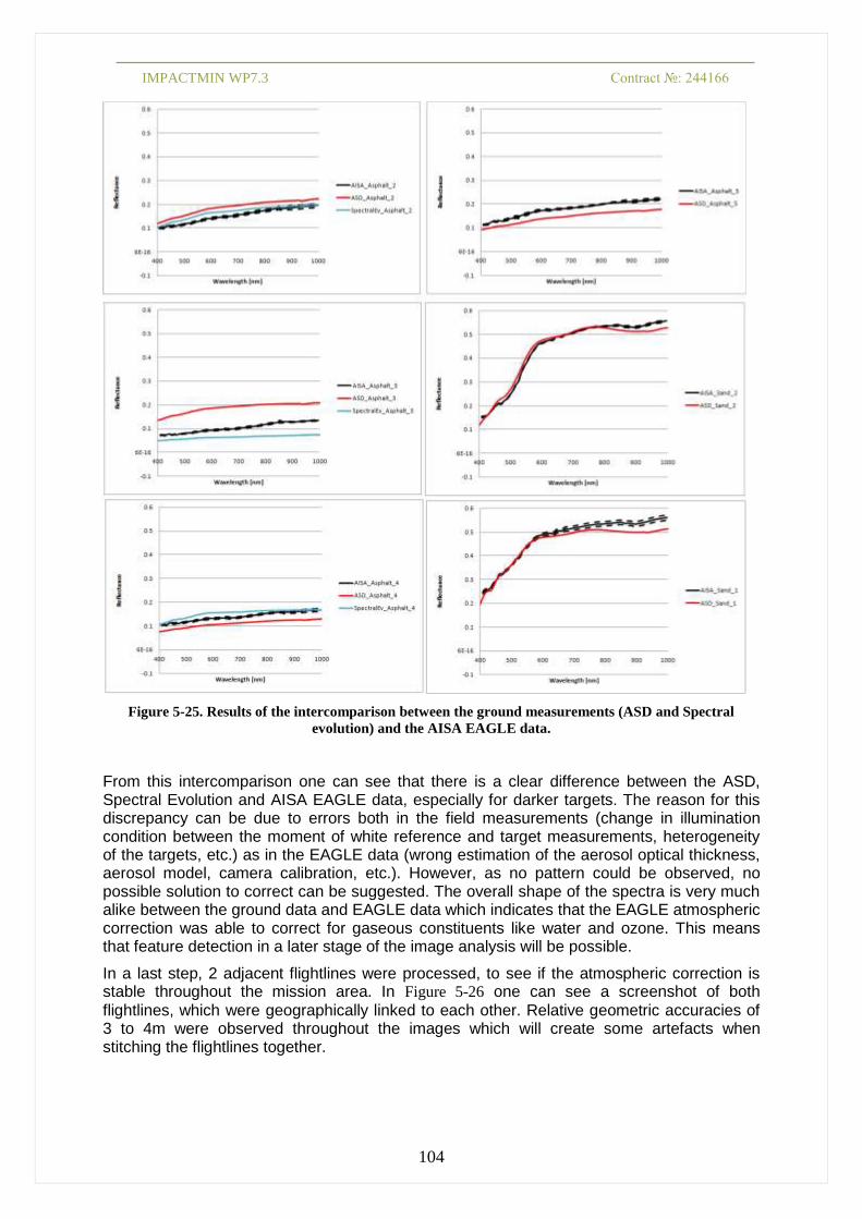
IMPACTMIN WP7.3 Contract №: 244166
104
Figure 5-25. Results of the intercomparison between the ground measurements (ASD and Spectral
evolution) and the AISA EAGLE data.
From this intercomparison one can see that there is a clear difference between the ASD, Spectral Evolution and AISA EAGLE data, especially for darker targets. The reason for this discrepancy can be due to errors both in the field measurements (change in illumination condition between the moment of white reference and target measurements, heterogeneity of the targets, etc.) as in the EAGLE data (wrong estimation of the aerosol optical thickness, aerosol model, camera calibration, etc.). However, as no pattern could be observed, no possible solution to correct can be suggested. The overall shape of the spectra is very much alike between the ground data and EAGLE data which indicates that the EAGLE atmospheric correction was able to correct for gaseous constituents like water and ozone. This means that feature detection in a later stage of the image analysis will be possible.
In a last step, 2 adjacent flightlines were processed, to see if the atmospheric correction is stable throughout the mission area. In Figure 5-26 one can see a screenshot of both
flightlines, which were geographically linked to each other. Relative geometric accuracies of 3 to 4m were observed throughout the images which will create some artefacts when stitching the flightlines together.
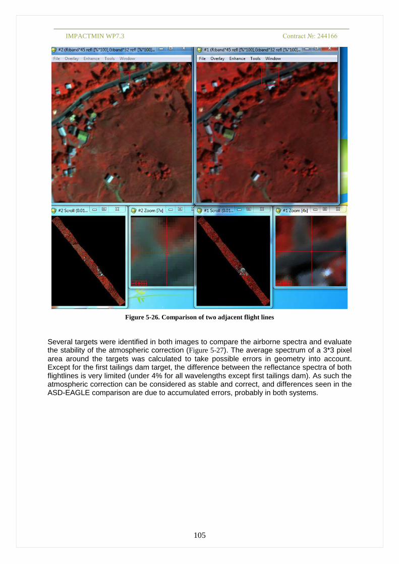
IMPACTMIN WP7.3 Contract №: 244166
105
Figure 5-26. Comparison of two adjacent flight lines
Several targets were identified in both images to compare the airborne spectra and evaluate the stability of the atmospheric correction (Figure 5-27). The average spectrum of a 3*3 pixel
area around the targets was calculated to take possible errors in geometry into account. Except for the first tailings dam target, the difference between the reflectance spectra of both flightlines is very limited (under 4% for all wavelengths except first tailings dam). As such the atmospheric correction can be considered as stable and correct, and differences seen in the ASD-EAGLE comparison are due to accumulated errors, probably in both systems.

IMPACTMIN WP7.3 Contract №: 244166
106
Figure 5-27. Spectral comparison of two adjacent flightlines on 6 targets.

IMPACTMIN WP7.3 Contract №: 244166
107
6 Interpretation of results of the hyperspectral measurements and remote sensing
6.1 Interpretation of sediments, soils and rocks characteristics
6.1.1 Stream sediments spectra In Figure 6-1 we have plotted the distribution for the spectral ratio R759/R937 nm, which is indicative for the size of the Ferric Iron absorption feature in the reflectance spectrum, and hence for the amount of iron-oxide/hydroxide in the stream sediments.
This figure shows high iron contents below the dumps south of the open pit, below the tailings dam, and at discrete points in the main stream flowing from the village. Those discrete spots coincide with the convergence of drainage coming from the open pit and underground galleries with the main stream.
A similar picture is shown by the pH suggesting a correlation between pH and Iron-oxide concentration in stream sediments. This correlation is confirmed by the trend in Figure 6-2a,
which shows an increasing Iron-oxide concentration with decreasing pH.
Lead and in particular Cadmium seem to show a positive correlation with the Iron oxide index (Figure 6-2b, c), whereas Cu, Zn and Ni seem to show a weak negative correlation (Figure
6-2d-f). When plotted on the map (Figure 4-19), these elements show enhanced values in the
direct surroundings of the deposit.

IMPACTMIN WP7.3 Contract №: 244166
108
Figure 6-1. Plots of the spectral Iron-oxide index, pH, Lead –content and Copper content of the stream
sediments around the deposit.
Figure 6-2. Plots of pH, Cd, Pb, Zn, Cu and Ni in stream sediments against the ratio of spectral
reflectances at 759 and 937 nanometers.

IMPACTMIN WP7.3 Contract №: 244166
109
6.1.2 Soil and rock spectra
A comprehensive description of the soil sampling procedure and analyses has been included in chapter 4. Samples of the main rock types occurring in the area have been collected from the mineralised zone, but also from outcrops at various distances from the deposit, where they occur mostly as individual boulders, steep edges such as scarps, riverbeds, roadsides, landslides, etc. (Figure 6-3). During the 2011 campaign we sampled outcrops in and around
the deposits for spectral analysis with the ASD-fieldspec spectrometer in order to identify the mineralogy of the hydrothermally altered rocks and their direct surroundings. During the 2012 campaign we took solar reflectance measurements of both hydrothermally altered and unaltered rocks with the Spectral Evolution PSR-3500 spectroradiometer for correlation with the WV2-imagery and the Airborne Hyperspectral imagery. The rock samples have been only spectrometrically analysed.
Figure 6-3. Typical example of rock outcrops around the deposit (a, b and c), and other outcrops, such as
individual boulders (d), scarps (e) and landslides (f).
The first step in our interpretation of the data involved a visual interpretation of the soil and rock spectra in order to determine the spatial distribution of minerals that are possibly related to the formation or presence of the deposit. Those minerals are Illite, Kaolinite, Goethite and Jarosite.
Illite is always related directly to lithology. It can be formed as a primary mineral during formation of the regional rocks, and it can be formed during hydrothermal processes that led to the formation of the Rosia Montana deposit. Our data (Figure 6-4) do not show a very clear
pattern but it suggests that both “types” of illite are present. We see a very clear cluster of illite-bearing soils associated with the deposits and their immediate surroundings, which is suggestive of hydrothermal sericitic alteration. But we also observe illite in the regional rocks, and these illites are probably representative of original mineralogy of certain types of lithology.
Note that the different colours of the symbols represent the strength of the diagnostic feature for each mineral, and not the abundance of that mineral.

IMPACTMIN WP7.3 Contract №: 244166
110
Figure 6-4. Maps showing the presence of minerals in soil and rock samples that are possibly related to
the formation of the deposits. (a) illite, (b) kaolinite, (c) goethite and (d) jarosite.
The distribution of kaolinite shows a very clear spatial relationship with the deposits, and it is therefore likely that this mineral is somehow related to the presence of the mineralization. This can be in two different ways. In the first place kaolinite can be formed directly as a result of relatively low temperature acidic hydrothermal alteration (argyllic alteration). In the second place kaolinite can be formed as a result of weathering of feldspars that are present in the rocks. Those feldspars can be primary lithologic (e.g. in magmatic rocks), or hydrothermally formed during the so called potassic alteration. In this particular case we have the impression that most of the kaolinites that we find are formed by alteration of feldspars that were present in the magmatic rocks that host the deposit, and therefore indirectly related to the genesis of the deposit.
Goethite seems to be dominant in and around the deposits, where it is probably formed by weathering of sulphide minerals. There are however other locations, unrelated to the deposit, where goethite is observed, and we suspect that this is related to lithological differences.
Jarosite, which is formed directly by weathering of sulphide minerals, is indicative of very low pH-values (pH 1-2), and is exclusively found within the known deposits.

IMPACTMIN WP7.3 Contract №: 244166
111
Above we have shown which minerals appear to be related, at least to some extent to the deposits. However, visual interpretation of spectra is a subjective method, and in order to be able to identify subtle changes in proportions and types of minerals present, and to determine if proportions of certain minerals change as a function of proximity to the deposit, we have to use other methods, based on numerical analysis of the spectra.
In Figure 6-5 we have presented the plots showing the relative proportions of iron-oxides
and/or jarosite and white mica and/or kaolinite using the relative depth of the diagnostic features at approximately 900 nm (iron-oxides and jarosite) and at approximately 2200 nm (white mica and kaolinite).
For calculation of the depth at 900 nm we have resampled the spectrometer spectra to WV2-spectra, because this makes it easier to correlate this ratio to Worldview imagery. This does not apply for the 2200 nm-feature, since this is outside of the spectral range of WV2.
The results show a very clear correlation of the feature strengths of these two groups of minerals with the distance to the deposits, with highest values right at the deposits.
However, both groups of minerals also show slightly enhanced values in the lower left (south-west) corner of the area. It is not clear how this should be interpreted, but since there seems to be a mineralogical similarity with the deposits at Rosia Montana, it could be interesting to check if there is any hydrothermal alteration in that area.
Figure 6-5. Depth of the 900-nm feature (left) using the ratio of bands750 nm/900 nm, and of the 2200 nm
feature (right). For the 900 nm-feature we have resampled to the corresponding WV2-bandpositions.
Depth of the 2200 nm-feature has been computed on the basis of the relative depth in the hulled-spectrum
using The Spectral Geologist (TSG). At the top we have plotted lab-spectra for the relevant minerals that
show absorption features at these wavelengths.

IMPACTMIN WP7.3 Contract №: 244166
112
6.1.3 Soil chemistry
A selection of representative soil samples from the 2011 and the May-2012 campaigns was analyzed for the following elements: Cu, Pb, Zn, Cr, Ni, Cd and the pH. The purpose of the chemical analyses was:
a) to determine if the soil chemistry shows any specific patterns in relation to the mineralization,
b) to study possible correlations between soil chemistry and spectral properties of soils, and
c) to determine if there are diagnostic variations in vegetation health that may be related to soil chemistry.
The various metal contents in soils and the pH of the soils are plotted in Figure 6-6. In
general, these plots do not show a very clear or systematic pattern for any of the elements analysed, and soils covering the Orlea and Jig areas, north of the main deposit, display rather strong contrasts.
However, if we compare the results of the chemical analysis with the results of the spectral analysis of the same samples some interesting relations seem to emerge (Figure 6-7).
Figure 6-6. Plots of the spatial distribution of (a) Copper, (b) Lead, (c) Zinc, (d) Cadmium, (e) Chrome
and (f) pH.

IMPACTMIN WP7.3 Contract №: 244166
113
In these plots we seem to observe that there is no systematic variation as far as the regional samples are concerned.
However, the samples that are collected close to the deposits seem to display quite distinct trends, especially when compared to the regional samples. The pH diagrams (Figure 6-7a, g)
show that with increasing proportions of iron-oxides and white micas, the soils become more acid. This can probably be explained by the fact that the more altered rocks, which underwent sericitic alteration, contain more illite and also contain more sulphides. As a result of weathering the sulphides will decompose into iron oxides and jarosite, accompanied by a decrease in pH, whereas the illite is stable during weathering and stays preserved in the soils, hence reflecting the original mineralogy of the altered rocks.
Figure 6-7. Relationship between (a-f) the spectral Iron-oxide index (WV6/WV8) and some relevant
chemical parameters, and between (g-l) the depth of the 2200 nm absorption feature and the chemical
parameters. The blue symbols represent the (regional) samples collected in May 2012, and the red
symbols represent samples collected in 2011 on or near the deposits.

IMPACTMIN WP7.3 Contract №: 244166
114
6.1.4 Mapping soil and grassland variations using the Worldview2 imagery
The basic concept of using remote sensing data for monitoring environmental impact in this area has two major aspects
1) Identification of differences within one single image, or in other words, a stationary
situation, at one certain time
2) Identification of changes between images from different acquisition dates
In the foregoing sections we have described how soil composition and mineralogy change in relation to underlying geology, and how these changes can be identified using spectral information.
While the spectral variation of soils as a result of changing mineralogy is certainly a key-parameter that we would like to be able to map using remote sensing data, the situation is significantly more complicated, because most of the soil exposures occur in grasslands, and in many of these grasslands the amount of exposed soil is relatively small.
As illustrated before, the variation in grasslands is fairly significant. While much of the observed variation can be related to differences in land-use such as crop-rotation, harvesting, irrigation, hay production, grazing, etc., there are also variations that clearly are related to natural factors such as drought, soil fertility, topography, bioturbation, etc.
As all these factors interact with each other, the mapping of subtle spectral variations in soils due to environmental impact, using remote sensing imagery is not a trivial task.
In the previous sections we have used spectral data collected by contact probe analysis, which means that the measurements were made under ideal conditions, on a very small (less than 1cm2) and relatively homogenous surface. The pixel of a WV2-image with 2m-resolution will be at least 40 thousand times bigger than a single contact probe reading. Except for places with well exposed bare soil, which are relatively rare, most surfaces are a mixture of grass with varying proportions of soil exposed, and this implies that each pixel in the WV2-image will represent a mixture of vegetation spectra and soil spectra. It is therefore unlikely that pure soil spectra and image spectra are directly comparable.
This is very clearly illustrated when we compare the spectral reflectance of soils measured with the contact probe, with the corresponding WV2-band value of the image pixel where the sample was collected (Figure 6-8). In order to be able to make this comparison, we resampled
the contact probe spectra to the respective WV2-band positions using the Envi spectral library resampling tool.
As described in a previous section, during the different field-campaigns we sampled in different parts of the area and different types of samples were collected (see section on soil sampling). In order to assess what impact the different sampling environments have on the correlation with the WV2-spectra, we have represented the different groups of samples with different symbols.
The plots reveal that for bands 1-5 the image spectra are generally darker than the contact probe measurements, whereas for band 6 most samples correlate reasonably well with WV2-

IMPACTMIN WP7.3 Contract №: 244166
115
data, and bands 7 and 8 are brighter than expected on the basis of the contact probe measurements.
Compared to most rocks and soils, vegetation has lower reflectances in the WV-bands 1-5 (see spectral graph in Figure 6-9) and higher reflectances in WV-bands 7-8, and therefore we can expect that mixing soils with vegetation will have the effect observed in Figure 6-8 for the
respective bands.
The wide scatter in these plots, especially for the rock samples (pink symbols) and the soil samples in vicinity of the deposits (red triangles) is probably a consequence of the fact that contact probe measurements do not adequately represent the inhomogeneous nature of the materials measured.
The effects of vegetation become more obvious when we compare the various band ratios (Figure 6-9). Band ratios are often considered very effective for mapping of subtle spectral variations in rocks and soils (see e.g. Figure 6-5) as well as vegetation, and in order to be
able to make a correct interpretation of the band ratio images, it is important to have a good understanding of the factors that can influence the band ratios.

IMPACTMIN WP7.3 Contract №: 244166
116
Figure 6-8. Plots showing the relation between the spectra from contact probe samples and the
Worldview2-spectra for the corresponding image pixels. In order to correlate the contact probe spectra
with the WV2-spectra, the former have been resampled to the respective WV2 band positions. Rock
samples 2011 are mostly taken from locations in or near the deposits. Soil samples 2011 are also taken
mostly at or near the deposits. Soil samples May 2012 are regional soil samples, collected on profiles in
grasslands. Soil samples July 2012 are taken in the transitional zone between the May 2012 and the 2011
soil samples, mostly from fairly well exposed soils.

IMPACTMIN WP7.3 Contract №: 244166
117
Figure 6-9. Comparison of band ratios for contact probe spectra and WV2-spectra. These are band ratios
that are often considered useful to map subtle variations in WV2-imagery. The symbols are the same as in
figure 29. For a better understanding of the meaning of the band-ratios, we have added a plot with the
WV2-spectra for representative surface materials. These spectra have been obtained by resampling
USGS-reference library spectra to WV2- band positions.
These figures very clearly illustrate how sensitive most of the band ratios, in particular WV4/WV5, WV5/WV6 and WV5/WV7, are with respect to vegetation. WV6/WV8 is also affected, but the general trend observed for the contact probe measurements seems to be well preserved.
The plot of the WV5/WV2 ratio reveals a completely different problem: The fact that the band ratio for the contact probe measurements is much lower than the ratio for the corresponding WV2-pixels is probably caused by an instrument problem. All 2011 samples were measured with an ASD spectrometer, whereas all 2012 samples were measured with a Spectral Evolution spectroradiometer. It was known our ASD was unstable in the shorter wavelength region (350 – 600 nm), causing the reflectance measurements in this region to be too high. Since this wavelength region corresponds to the WV bands 1-3, band ratios such as WV5/WV2 will be too low.
Fortunately this problem does not seem to exist for the wavelengths longer than 600 nm, and the variation for the band ratios involving Worldview bands 4-8 are as expected for bare soils and rocks.

IMPACTMIN WP7.3 Contract №: 244166
118
In 2012 we replaced the ASD spectrometer with a Spectral Evolution Spectroradiometer, and this allowed us to collect solar reflectance measurements in addition to contact probe measurements. During the field campaign in June-July 2012 we revisited many places that we had sampled before in order to take solar surface reflectance measurements of the locations (Figure 6-10).
Since solar reflectance measurements collect the spectral information over a much larger surface (in this case approximately 0.15 m2) than the contact probe measurements, we expect that the solar reflectance spectra will therefore correspond better to the WV2-spectra.
Figure 6-10. Locations of solar reflectance measurements collected between June 22 and July 4, 2012, and
the locations where samples were taken for contact probe analysis. In this plot we made a distinction
between solar reflectance targets that consisted for more than 90% of exposed soil with minor grass, and
(grassland) targets with a ratio between 0% and 90% exposed soil.

IMPACTMIN WP7.3 Contract №: 244166
119
Figure 6-11. Plots showing the relation between the solar reflectance spectra collected for soils and rocks
in July 2012 and the Worldview2-spectra for the corresponding image pixels. In order to correlate the
spectroradiometer spectra with the WV2-spectra, the former have been resampled to the respective WV2
band positions.
The results (Figure 6-11) indicate that the correlation with the WV-image spectra improves significantly for the solar reflectance measurements, compared to the contact probe measurements, the amount of scatter in the plots is significantly reduced, and there are significantly more samples that plot close to the line with a coefficient of 1.

IMPACTMIN WP7.3 Contract №: 244166
120
The green “tail” trending away from this line that is visible in particular in the plots of bands 3-5 indicates that these samples contain sufficient soil for detection with the spectrometer, but not enough for detection with the WV2-image.
The plots of the band ratios (Figure 6-12) for the solar reflectance measurements reveal some
very interesting patterns. The most interesting pattern is best discussed on the basis of the WV5/WV6-ratio (Figure 6-12c). From the spectral plot (Figure 6-12f) we can conclude that this ratio will be high for bare soils and rocks, and low for vegetation. We would expect that there will be a trend of decreasing ratio-values with increasing proportions of vegetation and that this trend will be more or less linear, with the result that all samples would plot near the line with coefficient 1.
However, this is not the case: Starting at the origin, we find the green symbols that represent samples with dominantly vegetation. Those green symbols display a horizontal trend, which means that while we observe the increasing soil proportions in the solar reflectance spectra, we cannot detect them yet in the W2-imagery. Only when we have 90% soil or more, we start noticing the presence of soils in the WV2-data.
The same trend is visible in all the band ratio plots except for WV5/WV2. However, this plot shows that all samples form one big cloud, and we cannot discriminate between soils and vegetation on the basis of this ratio.
The trend that we described above has direct consequences for our analysis of the remote sensing imagery, as it clearly shows the inherent limitations with respect to the spatial resolution.

IMPACTMIN WP7.3 Contract №: 244166
121
Figure 6-12. Comparison of band ratios for solar reflectance spectra and WV2-spectra. These are band
ratios that are often considered useful to map subtle variations in WV2-imagery. The symbols are the
same as in figure 32. For a better understanding of the meaning of the band-ratios, we have added a plot
with the WV2-spectra for representative surface materials. These spectra have been obtained by
resampling USGS-reference library spectra to WV2- band positions.
In order to obtain some more insight in the spectral variations within different types of grasslands, and to improve our understanding of the consequences of mixing different types of grass cover with different proportions of soil, we have studied the spectra of different mixtures in the four main grassland types: a) Grasslands with long, uncut grass; b) grasslands with short recently cut grass; c) grasslands with different proportions of dry grass and d) grazing lands with short grass (Figure 6-13).
This understanding should help us to assess more effectively when we may start seeing soil signatures in the grasslands, and when we may see other features that are spectrally similar to soils.

IMPACTMIN WP7.3 Contract №: 244166
122
Figure 6-13. Spectral mixtures for different types of grasslands: a) Long green grass with different
proportions of soil exposed; b) Recently cut green grassland with different proportion of soil exposed; c)
Recently cut grassland with different proportions of dry grass; d) Grazing land with short grass and
different proportions of soil exposed.
The data show that for the long grassland (Figure 6-13a) measurements with 50% soil still have a significant vegetation signature and we will probably not be able to identify the soils in these grasslands on the basis of the WV2-imagery. The detection of soils would be slightly more efficient if we also had spectral coverage in the SWIR-region, since the 2200 nm – clay absorption feature is fairly clear in the measurement with 50% soil. For the recently cut green grassland (Figure 6-13b) the spectrum at 25% soil is less affected by the presence of grass.
This figure indicate that if short, recently cut grass has more than 25% soil exposed, we will probably be able to recognize this in our image spectra. A very weak clay-feature at 2200 nm appears in the spectrum of 10% soil exposure. For the recently cut grass with dry grass (Figure 6-13c) we see a significant change in the spectrum in the presence of as little as 25%
dry grass, and on the basis of these spectra we expect that grasslands with more than 25% dry grass will appear very similar to exposed soil. For grazing land (Figure 6-13d) the situation
is most favourable for mapping soils. The graph suggests that for grazing lands we will be able to map soils when present in proportions as low as 25%.

IMPACTMIN WP7.3 Contract №: 244166
123
6.1.5 Image classification of soils
As described above, the variations in the appearance of grasslands in the imagery will depend on a complex interaction of human and natural factors. It is important that we are able to map these variations, because this will provide us with the tools needed to understand and monitor subtle changes over longer periods of time.
Our study of the correlation between field spectra and image spectra clearly demonstrates that image resolution is a key factor that determines our ability to map these subtle variations and changes. The fact that the spectral response in the WV2-imagery is so strongly dependent on the proportion of soil in a pixel implies that we cannot simply compare spectra from different grasslands, but that we have to divide the grasslands into classes on the basis of the expected proportion of soil exposure. The only way we can do this is by looking at the greenness of the grasslands, assuming that browner colours correspond to higher proportions of exposed soil.
We are aware that this is not entirely realistic, as the brown colour of the grasslands is also frequently associated with grasslands that have recently been cut (see Figure 6-14 and Figure
6-15). In those cases it is more likely that the brown colours are a combined result of short
dry brownish grass, and – because of the shorter grass – increased proportions of exposed soils. However, since the spectra of dry grass and clayish soils are very similar (Figure 6-13), especially in the VNIR, they are very hard to distinguish.
The images displayed in Figure 6-14, Figure 6-15 give some examples of situations where the
high resolution Smartplanes imagery provides information that is essential for the understanding of the land-use processes that we are actually observing in the WV2-imagery. These images contribute significantly to our ability to interpret the spectral variations in the context of the dynamics of the surface cover.

IMPACTMIN WP7.3 Contract №: 244166
124
Figure 6-14. Comparison of the July 2012 WV2 imagery and the Smartplanes imagery for various types of
soil exposures a-b: red arrows mark examples of recently cut, and dried grasslands. Hay stacks are clearly
visible on the Smartplanes image; Blue arrows indicate exposed soil in a crop field. c-d: Red arrows mark
examples areas that appear to be in the process of being cut. Blue arrows mark examples of exposed soil.

IMPACTMIN WP7.3 Contract №: 244166
125
Figure 6-15 e-f: The red arrows mark a strange zoning in the grasslands for the WV2-image. This zoning
is not visible in the Smartplanes image. We suspect that in this area the cutting of the grass is still in
progress, and that in the brown areas grass has been cut in the four days lapse between the acquisitions of
the two datasets, whereas the greener part has probably been cut more recently. The blue arrows mark
exposure of rocks and soil. g-h: image of typical grazing land with very short grass, and many small spots
with exposed soil (see also figure 6-12. The blue arrow marks a small pile of gravel. The other white spot
on the Smartplanes image is our field-van.
Dividing the grasslands into classes on the basis of the inferred proportion of soil exposure is best done using the relationships between WV2-bands 5 and 6, or 5 and 7, as they appear to be most sensitive to changing proportions of soil and grass (Figure 6-12). On the basis of
tests performed with the WV2-image acquired in 2012 we decided that the NDVI (WV5+ WV7/WV5-WV7) was most suitable to classify the surface. We classified the surface into four classes ranging from 100% soil to almost no soil in an empirical manner using the following threshold values:
NDVI < 0.301: No vegetation (Figure 6-16, red pixels)
NDVI 0.301 – 0.601: Some vegetation (Figure 6-16, orange pixels)
NDVI 0.601 – 0.681: estimated 50/50 vegetation/soil (Figure 6-16, green pixels)
NDVI 0.681 – 0.748: some soil (Figure 6-16, blue pixels)
NDVI > 0.748: pure grass

IMPACTMIN WP7.3 Contract №: 244166
126
Figure 6-16. Results of the WorldView2 land-cover classification using the NDVI. Arrows mark the
locations discussed in the previous section. For explanation of the colours, see text above.
The results (Figure 6-16) show that this approach can effectively be used to subdivide the
exposed surface into different classes that reflect the status of soils and grasslands. The results of this procedure can be used to map spectral differences between soils that occur within the same soil class (Figure 6-17).

IMPACTMIN WP7.3 Contract №: 244166
127
As demonstrated before, the presence of vegetation has a clear effect on several band ratios, and even though for the WV6/WV8 ratio the effect is not as strong as for other ratios, we have to evaluate the results separately for each of the different classes of soil-exposure (Figure 6-18) in order to make sure that we do not mix up different phenomena.
The results show very clearly that for the class of the bare soils, most of the enhanced WV6/WV8 values are associated with the areas of mining activity. For the class of the soils with some vegetation we see however that the ratio values are generally much lower. When comparing the results with the spectral measurements we see that there is a fairly good correlation between the image data and the solar reflectance measurements (Figure 6-18a). For the contact probe data (Figure 6-18b) we observe that the contact probe values are in
reasonable agreement with the image data for most of the bare soil class. However, for the more vegetated areas the image values are consistently lower than the contact probe values. As demonstrated in previous sections, this discrepancy is a result of the presence of vegetation in the pixel. The results confirm that with increasing proportions of vegetation, the original soil spectra become increasingly less visible. However, the positive side is that in the case of environmental impact leading to deterioration of the grasslands, and hence better exposure of soils, we will automatically be able to detect this process. Since most of the soils are richer in iron oxides than expected on the basis of the current image data, the WV6/WV8 ratio will by definition increase if the proportion of vegetation in a pixel decreases.

IMPACTMIN WP7.3 Contract №: 244166
128
Figure 6-17. WV2 band ratio (6/8) results for the 2012-image for soil class 1 (bare soils, top) and soil class
1 and 2 (bare soils and scarce vegetation respectively, bottom).

IMPACTMIN WP7.3 Contract №: 244166
129
Figure 6-18. Field spectra were resampled to WV2-bands, and the plots show the ratio of the WV6/WV8
for the solar spectra (top) and for the contact probe spectra (bottom) overlain on the same ratio for the
WV2-image. The same colour scheme has been used for the image data and the field spectra.

IMPACTMIN WP7.3 Contract №: 244166
130
6.1.6 Time series analysis and temporal monitoring
The procedure that we propose for the analysis of the satellite imagery is very suitable to monitor temporal changes such as proportions and mineralogical composition of exposed soil as indicators for vitality of grasslands over time using multi-temporal imagery provided that the atmospheric correction of the images is performed correctly. Proper atmospheric correction is essential otherwise it is not possible to maintain the same thresholds throughout the time-series of images.
Monitoring of changes in proportions of soil/grass for grasslands is important because these changes may be used as indicators for degradation of the environment due to mining activities. Increased environmental pressure may lead to deterioration of the grassland-ecosystem, and hence to increasing proportion of exposed soil at the expense of grass cover. Monitoring these changes can be achieved by comparing the maps for each soil class over subsequent years. In our example, we have generated soil-proportion maps for three consecutive years (2010-2011-2012) using WV2-imagery (Figure 6-19). Combination of each
class into an RGB image for the three consecutive years will show very clearly where changes occurred over time. Clearly one has interpret these results with care, because such changes can also be related to climatic conditions (e.g. dry vs rainy years) and to changes in land-use (e.g. grazing-land vs hay-land) As demonstrated in a previous section, from a spectral point of view the variations in iron-oxide/jarosite content and white mica and clay (illite, kaolinite) content form the most prominent mineralogical changes in the soils in the Rosia Montana area. In contrast to the micas and clays, which probably represent primary lithology, Iron oxides and Jarosite are related to weathering Several authors (Hill, 1993; Richter et al., 2006) have demonstrated that one of the more noticeable effects of soil degradation is an increased weathering due to deterioration of the protective vegetation layer and removal of organic-rich topsoil. Increased and prolonged weathering will result in alteration of the original minerals into clay minerals such as montmorillonite, nontronite, beidellite, halloysite, etc. During the weathering process iron is released from these minerals and becomes oxidized, and the ferric iron will subsequently be accumulated in the residual soils in the form of oxides and hydroxides. In the presence of pyrite, even minerals such as jarosite may be formed. These secondary Iron minerals can be mapped very effectively using imaging spectroscopy (Richter et al, 2007). This implies that we will be able to monitor potentially important changes in the condition of soils over time by estimating the proportion of Iron in soils. Earlier in this study we have demonstrated (Figure 6-5) that, using resampled soil spectra, the band ratio of WV(6)/WV(8) is a very effective estimator of the proportion of Iron-oxides and/or Jarosite in soils.
In order to demonstrate the procedure to monitor the changes in soil mineralogy over time, we have calculated the difference between the WV6/WV8 band ratios of 2010 and 2012, for each individual soil class. The results show (Figure 6-20) that for the bare soil class there has
been almost no change in the areas that were strongest affected by the past mining (the open pits and the tailings dam). Some other locations however show fairly significant change. These areas correspond with areas that have recently been stripped from vegetation

IMPACTMIN WP7.3 Contract №: 244166
131
For the second soil class (with some grass cover), there appears to be more differentiation. For example there is a zone north of the town of Rosia Montana, where we have mapped increased Fe-oxides contents in soils.
Figure 6-19. Distribution of soil classes for 2012 (a), 2011 (b) and 2010 (c).By combining a specific soil
class for each year into an RGB colour composite we can visualize the changes for a specific soil class over
time (figs. d-g). Fig. d: (Red) distribution of bare soil in 2012, (green) distribution of bare soil in 2011,
(blue) distribution of bare soil in 2010. Fig. e: same for the second class (soils with some vegetation). Fig. f:
same for the third class (soils with significant vegetation). Fig. g: same for the fourth class (mostly
vegetation with some soil)

IMPACTMIN WP7.3 Contract №: 244166
132
Figure 6-20. Difference of the Ratio WV6/WV8 between 2010 and 2012 for bare soils (top) and soils with
some grass-cover (bottom). Higher values indicate an increase of Fe-oxide content in 2012 compared to
2010.

IMPACTMIN WP7.3 Contract №: 244166
133
6.1.7 Hyperspectral mapping of soils
The main purpose of the acquisition of the hyperspectral imagery was the ability to map changes in vegetation stress. However, because of the high spatial and spectral resolution of the data we expected that they will be also very valuable for mapping variations in proportions of soil/grass in grasslands as well as subtle compositional changes of soils with respect to the presence of iron oxides and jarosite. Classification of soil/grassland proportions In a previous section we have already noted for Worldview2-imagery that mixing relatively small amounts of vegetation with soils can strongly influence the resulting image spectra (e.g. Figure 6-12). A similar comparison (Figure 6-33) between surface measurements and the hyperspectral image spectra demonstrates that increasing the spatial resolution from 2m (WV2) to 50 cm (hyperspectral) hardly makes any difference;
Figure 6-21. Left: comparison of WV2-pixel signatures with corresponding field spectra; Right:
comparison of AISA-Eagle pixel signatures with corresponding field spectra.

IMPACTMIN WP7.3 Contract №: 244166
134
The data show very clearly that also for the 50 cm imagery, relative small amounts of vegetation have a significant impact on the image spectra. However, a major difference with the Worldview2 imagery is that the likelihood of finding exposed patches of bare soil with size of 0.25m2 will be significantly higher than finding exposed bare soil patches with a size of 4m2.
Hence we expect that potential of mapping small patches of bare soil will be much higher when using the 50 cm hyperspectral data. This can be investigated by comparing the classification for bare soils from WV2-imagery and AISA-Eagle imagery (Figure 6-34), using the same methodology of thresholding of the NDVI. As a reference, we have also generated a bare soil map from the Smartplanes imagery using a spectral angle mapper classification.
Figure 6-22. Top: Results of Spectral Angle classification for Smartplanes imagery. Red pixels represent
exposed bare soils. Bottom: Results of bare coil classification using for WV2 (blue pixels) and
hyperspectral (red pixels), based on thresholding of the NDVI. The grid interval is 50m.

IMPACTMIN WP7.3 Contract №: 244166
135
This figure clearly demonstrates that the hyperspectral imagery indeed enables us to map much smaller exposures of bare soil. It is very interesting though to note that the Smartplanes imagery yields by far the most detailed and accurate map of exposed soils (Figure 6-22 top, red pixels).
Mapping of Iron oxides in soils In the previous section we demonstrated that we can successfully map iron oxides in soils using WV2 band ratios WV6/WV8, but that discriminating between goethite and jarosite is much less simple. While the main absorption feature of jarosite is located in the SWIR (around 2250nm) the laboratory spectra (Figure 6-23a) show that there is enough spectral difference in the VNIR-
range differentiate between Jarosite and Goethite. However, the characteristic difference between the jarosite and goethite spectrum in the VNIR – the shift of the position for the maximum from 760 nm to 710 nm – cannot be mapped in WV2-imagery (Figure 6-23b). The other diagnostic features of these minerals are
the broad absorption features around 650 nm and 900 nm. Unfortunately these features are shared by both minerals, and as jarosite normally does not occur on its own (especially at the scale of a WV2-pixel), but as a mixture with goethite, we can only assess the proportion of jarosite/goethite by looking at relative depth of these features. In the case of WV2-imagery this means that we can map secondary iron minerals in soils by looking at the ratio of WV6/WV8, and assume that larger WV6/WV8 band ratios may indicate larger proportions of jarosite/goethite in soils. Our hyperspectral imagery however makes it possible to look at the full VNIR-spectrum, and should be easier to directly map the diagnostic changes in the spectral curves related to the presence of jarosite and goethite in soils (see Figure 6-23c), using supervised classification on the basis of image-derived end-member spectra.
Figure 6-23. Spectra of Jarosite and Goethite from the USGS- spectral library and AISA-EAGLE
imagery.
After performing a Spectral Angle classification using the two end-member spectra (Figure
6-23c), we have thresholded the resulting rule-images, and combined the maps for jarosite and goethite into a composite mineral map (Figure 6-24). Overlain on this map are the
interpreted field spectra, showing the locations where jarosite was abundant (red symbols), weak (yellow symbols) and absent (blue symbols). In general there is a good correlation between the field spectra and the classified image, showing well defined Jarositic zones in the large (Cetate-Carnic) open pit and some smaller jarosite occurrences over the Vaidoia /Jig and Orlea orebodies.

IMPACTMIN WP7.3 Contract №: 244166
136
Figure 6-24. Results of supervised classification of the AISA-EAGLE hyperspectral imagery. Red pixels
indicate the presence of Jarosite, and blue pixels the presence of Goethite. The red symbols show the field
samples with a prominent jarosite signature, the yellow symbols show samples with a weak jarosite
signature, and the blue symbols are the samples without jarosite.

IMPACTMIN WP7.3 Contract №: 244166
137
Comparison with the WV2 Iron oxide classification Since the acquisition and processing of high-resolution hyperspectral imagery is very expensive compared to the cost of WV2-imagery (see Figure 6-31) it is important to evaluate
the potential advantages offered by the hyperspectral VNIR for Fe-oxide mapping as opposed to the lower cost WV2. In previous sections we have demonstrated that the VNIR hyperspectral-imagery can be used successfully to map Iron oxides and Jarosite. In its ability to map Jarosite in a more reliable manner, the hyperspectral data clearly give us an advantage compared to WV2. It can also be expected that iron oxides can be mapped more accurately and in greater detail with the hyperspectral data compared to WV2-imagery because of the much higher spatial and spectral resolution than Worldview2. This is quite important since this may make it much easier to detect and map processes of land degradation. For that reason we have compared the maps with relative iron-oxide abundances (Figure 6-25 and Figure 6-26) obtained from Worldview2 imagery (using the WV6/WV8 band ratio) and
hyperspectral imagery (using the ENVI spectral angle mapper). As a reference we have used the ultra-high spatial resolution Smartplanes data, since in those images we can visually identify the presence of iron oxides with great detail. As a small test, we have also made an attempt to perform a spectral classification of the Smartplanes imagery to see if it would be possible to map iron-oxides directly from normal natural colour airphotos. The classification was done using a simple spectral Angle mapper, and the results (Figure 6-25 and Figure 6-26)
demonstrate that these data are actually extremely accurate, and can be used very successfully to map iron oxides in soils.
Figure 6-25. Comparison of Iron-oxide classification on the basis of WV2 and Hyperspectral imagery for
an acid drainage outlet of the tailings dam. A: (top left): Smartplanes image; B: (top right) Classification
of WV2-imagery; C: (bottom left) Hyperspectral classification and D: (bottom right) Smartplanes
classification.

IMPACTMIN WP7.3 Contract №: 244166
138
Figure 6-26. Comparison of Iron-oxide classification on the basis of WV2 and Hyperspectral imagery for
the face of the tailings dam. A: (top left): Smartplanes image; B: (top right) Classification of WV2-
imagery; C: (bottom left) Hyperspectral classification and D: (bottom right) Smartplanes classification.
6.1.8 The pseudo-hyperspectral evaluation
The collected samples were analysed with an ASD FieldSpec reflectance spectrometer and the acquired spectra compared against USGS spectral library for classification purposes. Majority of the analysed samples fall into the intimate mixtures of iron oxide (hematite) and hydroxide (goethite), sulphides (jarosite, copiapite, scwhertmannite), clay minerals (kaolinite, illite, halloysite, montmorillonite), or other silicates (sericite, epidote) or feldspars (microcline). The intimate mixtures were resolved with principal component separation into mineral-dominant 4 bins, determined by the strength of the perceived absorption feature (e.g. broad 600-900 nm absorption for Fe minerals, 2200 nm for clays, etc.) and the categorized results divided into four bins: clays, iron oxides, hydroxides, sulphate minerals. The intensity of the particular group was determined through the depth of the particular band-center characteristic for the group (e.g. 2200 nm for clays) and then, using continuum-removed spectrum, cross-compared for the strength of the particular absorption feature on the scale of 1 through 10, where the “intensity vector” corresponded with the particular absorption minimum along the characteristic band minimum. The methodology from which the classification of spectral features has been adapted is presented in detail by Kokaly et al. (2007).
The resulting spectral groups, along with the GPS coordinates for the collected samples and with the particular intensity values were then imported into Geosoft’s Oasis Montaj database

IMPACTMIN WP7.3 Contract №: 244166
139
and treated like “intensity” values of a four-channel geophysical sensor (e.g. a gamma ray spectrometer). The intensity values were transformed into a “grid” using Krigging function and then displayed as ternary ratio images of grids, to show for the potential correlations. To make it easy to interpret these pseudo-spectral grids, the three of four dominant sources (FeO, Sulphate, Clay) or ratios of each (FeO versus FeOH or Clays versus Sulphate) can be combined into a ternary image. The ternary geophysical images are presented as a constituent-ratio map. Brightest colours are used for highest levels of Clay (cyan), Jarosite (magenta) and FeO (yellow) grading to black where lowest levels of all three are recorded, or red-green-blue primary colours where there are mixtures. White colours indicate that all constituents are at high concentrations. The values can also be displayed as point-source concentration values or ratios for comparison with other types of data (e.g. Worldview 2).
The results on Saliste waste-pile show increased concentration of sulphate minerals in the central and eastern portions of the pit. Other areas are relatively stabilized with clay minerals, but in the areas where the water-flow is encountered, sulphates and hydroxides are able to breach the clay cap and continue to be transported further. This is to be expected as the clays are relatively inert while the areas where sulphates values are higher tend to be coarser and sandier in appearance, facilitating their transport by the waters entering the tailings dam on the East.
Figure 6-27. Ternary image map of three main constituents of interest on Worldview 2 image data

IMPACTMIN WP7.3 Contract №: 244166
140
Figure 6-28. Ternary map and relative concentrations of jarosite overlapped on Smartplanestm
UAV
generated image and DEM.

IMPACTMIN WP7.3 Contract №: 244166
141
Figure 6-29. Relative abundance of clay, iron-oxide, and jarosite.
In the main area of the mine, the Cetate pit, the main concentration of sulfate minerals appears to be directly associated with the mineralization of vein stockwork and breccia targets and as such remains mainly concentrated within core of the pit. The other clays and iron-minerals are mainly on the periphery in the relatively wide-spaced alteration zone. The clay cap is concentrated mainly around dacite intrusives to the southeast. There appears to be very little emission from the pit itself and the majority of sulfate minerals appear to be fairly contained, with exception of the zone in the far west-northwest segment of the pit which indicates presence of jarosite on a hillside, which may drain downhill towards the ravine and creek leading towards Abrud River.

IMPACTMIN WP7.3 Contract №: 244166
142
Figure 6-30. Ternary map showing relative abundances of jarosite (green), FeO (red) and clay minerals
(blue) overlain on Google Earth image of Cetate pit, looking East.
The method shows that field spectroscopy and new visualization/gridding techniques are adequate in discerning problematic zones. The signal originates from the measurements made on the upper few centimetres of surface so it is representative of the geochemistry of the examined land surface. Soil formation processes such as erosion and transport by wind and water have concentrating or sorting effects on the relative abundance of the analysed classes across the landscape, but this type of sampling and imaging gives significant insight into these processes and the present pattern of surface mineralogy types. Even though it is more cumbersome to carry out these kinds of surveys, it shows how spectroscopy can be effectively used to create surface-mineral cover maps in a wider area of interest.

IMPACTMIN WP7.3 Contract №: 244166
143
6.1.9 Cost-benefit considerations In the previous section we have demonstrated that all three types of imagery (WV2, Hyperspectral, and Smartplanes) can be used to map variations in soil/grass coverage and to map the presence of iron oxides. We have identified limitations and possibilities at different scales and with different accuracies, and this allows us to select a particular type of imagery depending on the requirements of the end-user. Besides these technical aspects, also the cost of the data will form an important aspect that needs to be considered in the selection of the type of imagery that will be used in such a monitoring project. For that reason we have made an assessment of the cost for each data type per square km based on our experiences in Rosia Montana area. In order to investigate the cost per square km as a function of the size of the survey-area, we calculated the cost for two scenarios based on the actual costs that were made in this project:
a) a survey area of approximately 100 km2, which corresponded to the actual survey area in this project
b) a survey area of 10 km2
For the calculation of the costs we have used the following assumptions:
a) The hyperspectral survey has to be mobilised from Münster or a comparable place b) There are no “bad-weather days” c) Administrative costs (flight permitting, etc.) are included d) A Smartplane UAV would be available on site (owned by the mining company), which
means that there would not be mobilisation costs. e) The minimum coverage for Worldview2 imagery is 100 km2
The results of our computations demonstrate that for the scenario of 100 km2 (Figure 6-31a)
we see a logarithmic increase of cost per square kilometre as a function of resolution. However, for smaller areas (Figure 6-31b) we see that the hyperspectral survey becomes very expensive compared to the Smartplanes UAV survey. This means that for small areas it will be cheaper to use a UAV instead of a manned aircraft. According to our data, the break-even point lies around an area of 25 km2 The fact that a UAV-survey is so much more cost-effective for smaller areas invites us to investigate the possibilities of other sensors, such as the VNIR hyperspectral framing camera that has recently been developed by the Finnish Technical Research Centre, VTT. (Honkavaara et al. 2012, see also http://www.rikola.fi/tunable_optical_filter.htm)
Figure 6-31. Cost of data acquisition, pre-processing and analysis for WorldView2, Hyperspectral
imageryand Smartplanes imagery per square km. a: (left) for a scenario of 100 Square km and b: (right)
for a scenario of 10 square km.

IMPACTMIN WP7.3 Contract №: 244166
144
6.2 Monitoring vegetation stress
6.2.1 Monitoring vegetation stress – leaf level In this section, the impact of past mining activities on the health status of birch trees in the Rosia Montana area is investigated. In first instance, a statistical analysis is performed to define wavebands and waveband ratios that are able to spectrally distinguish birch leaves sampled in a polluted area from those in a remote area. The result of this analysis is afterwards applied on the whole birch leaves dataset gathered in June and August 2012. Finally, this work is extended to the airborne hyperspectral dataset, gathered in August 2012.
Figure 6-32. Birch trees in the study area and GPS measurement
In June 2012, 39 leaves of a birch tree located near the tailings dam in polluted area were spectrally sampled. Also a birch tree in a remote area was selected of which 40 leaves were spectrally measured.
Figure 6-33. Leaf spectral sampling with the plant-probe.

IMPACTMIN WP7.3 Contract №: 244166
145
The leaf spectra of both trees were used in a decision tree classification, from which the most appropriate waveband to distinguish the 39 polluted from the 40 non-polluted spectra, was obtained. The analysis resulted in the selection of waveband 706.8 nm with reflectance values lower than 0.16 belonging to the polluted tree and higher than 0.16 to the non-polluted tree. A classification accuracy of Kappa = 0.72 was thereby obtained. Since the selected waveband corresponded to the red edge inflection point (REIP), a more detailed analysis with derivative spectra was performed. From the derivative study, it seemed that a shift of the REIP existed to longer wavelengths in polluted areas. Those results were unexpected, since it has been shown previously that the maximum first derivative of grassland spectral signatures in the red-edge region yielded a significant, negative correlation with the total heavy metal concentration in the soil. Hypothesis in that study was that heavy metal contamination in the soil has a negative effect on the chlorophyll concentration of the leaves, which could not be seen in the trees under investigation.
However, when plotting the REIP values of all sampled trees on a WV2 image, a gradient toward lower REIP values is observed in the open pit area and its surroundings, which corresponds well with results published by other authors.
Figure 6-34. REIP values for all sampled birch leaves in Rosia Montana area
Furthermore, the decision tree classification with derivative spectra of the two selected trees showed lower derivative values at 2280 nm for polluted compared to non-polluted leaves (kappa=1).

IMPACTMIN WP7.3 Contract №: 244166
146
Figure 6-35. Derivative spectra of the polluted (purple) and non-polluted (green) birch leaves, with
horizontal grey lines indicating the most informative bands according to the outcome of the decision tree
classification.
It has been found in literature that this 2280 nm spectral region is influenced by the absorption of biochemicals, such as foliar nitrogen and lignin concentrations. Fourty et al. (1996) reported absorption peaks of nitrogen and lignin (Table 6-1) based on previous works
by Curran (1989) and Himmelsbach et al. (1988):
Table 6-1. Absorption peaks of nitrogen and lignin
Biochemical Absorbing Wavelength (nm)
Nitrogen 1020, 1510, 1730, 1980, 2060, 2130, 2180, 2240, 2300
Lignin 1120, 1200, 1420, 1450, 1690, 1754, 1940, 2262, 2380
In-depth literature analysis revealed a direct link between lignin and heavy metal content. Several authors reported that an increase in lignin content is considered as a common plant response to various environmental or stress factors, such as ozone (Cabane et al. 2004) or heavy metal (Diaz et al. 2001; Jbir et al., 2001; Dixon et al., 2002; Janas et al., 2002; Mandre, 2002; Winkel-Shirley, 2002; Jouili & Ferjani, 2003; Lin et al., 2005; Yang et al., 2007; Kovacik & Klejdus, 2008) exposure, which may induce or alter lignin synthesis.
Serrano et al. (2002) proposed the Normalized Difference Lignin Index
as index to asses lignin in native shrub vegetation with remote sensing data. They found out that NDLI provided consistent and significant results across vegetation communities and functional types. As a consequence, the NDLI index was calculated for the polluted and non-polluted tree leaves. It can be seen for Figure 6-36 that NDLI values of polluted leaves are
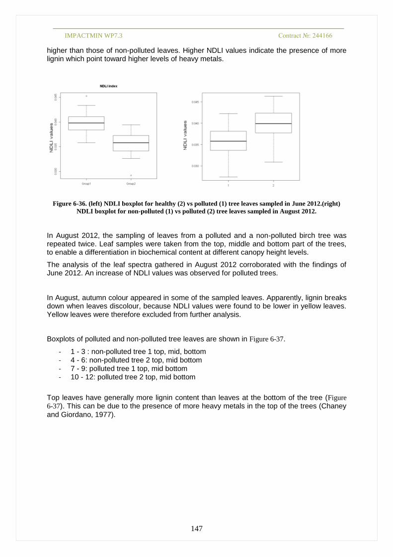
IMPACTMIN WP7.3 Contract №: 244166
147
higher than those of non-polluted leaves. Higher NDLI values indicate the presence of more lignin which point toward higher levels of heavy metals.
Figure 6-36. (left) NDLI boxplot for healthy (2) vs polluted (1) tree leaves sampled in June 2012.(right)
NDLI boxplot for non-polluted (1) vs polluted (2) tree leaves sampled in August 2012.
In August 2012, the sampling of leaves from a polluted and a non-polluted birch tree was repeated twice. Leaf samples were taken from the top, middle and bottom part of the trees, to enable a differentiation in biochemical content at different canopy height levels.
The analysis of the leaf spectra gathered in August 2012 corroborated with the findings of June 2012. An increase of NDLI values was observed for polluted trees.
In August, autumn colour appeared in some of the sampled leaves. Apparently, lignin breaks down when leaves discolour, because NDLI values were found to be lower in yellow leaves. Yellow leaves were therefore excluded from further analysis.
Boxplots of polluted and non-polluted tree leaves are shown in Figure 6-37.
- 1 - 3 : non-polluted tree 1 top, mid, bottom - 4 - 6: non-polluted tree 2 top, mid bottom - 7 - 9: polluted tree 1 top, mid bottom - 10 - 12: polluted tree 2 top, mid bottom
Top leaves have generally more lignin content than leaves at the bottom of the tree (Figure
6-37). This can be due to the presence of more heavy metals in the top of the trees (Chaney
and Giordano, 1977).

IMPACTMIN WP7.3 Contract №: 244166
148
Figure 6-37. NDLI boxplots for non-polluted tree leaves sampled from the top (1&4), center (2&5) and
bottom (3&6) of the trees and for polluted tree leaves sampled from the top (7&10), center (8&11) and
bottom (9&12).
Besides the leaves of the two (June 2012) and four (August 2012) selected birch trees, many more leaf samples were taken from, amongst others, small, medium, and large birch trees and hornbeam trees. NDLI values did not show significant differences between the different birch tree groups, but hornbeam did have a significant (Wilcoxon rank test p<0.001) lower lignin content compared to the birch trees (Figure 6-38).
Figure 6-38. NDLI boxplots for tree leaves sampled from small (1), medium (2) and large (3) birch trees
and for hornbeam (4) leaves sampled in August 2012.
NDLI values of all sampled birch leaf spectra were plotted on a WV-2 image (Figure 6-39), in
order to show their spatial distribution. Overall higher NDLI values can be observed for birch trees located near to or on the open pit area. Based on the spatial patterns, NDLI was found to be the best predictor for heavy metal stress out of a bunch of tested vegetation indices.

IMPACTMIN WP7.3 Contract №: 244166
149
Figure 6-39. Overview of NDLI values at different locations in the mining area
6.2.2 Monitoring vegetation stress – airborne level
A hyperspectral airborne flight campaign was set up in August 2012 (see previous section and Figure 5-20). The Eagle sensor provided 64 spectral bands in the VNIR spectral region
and a spatial resolution of 0.5 m. Since the airborne hyperspectral data are in the VNIR spectral domain, a first goal was to find in this domain a VNIR waveband or vegetation index closely correlated with the NDLI. It has to be noticed that this analysis is based on the assumption that NDLI is a good heavy metal stress indicator.
Birches wavelengths - NDLI
From a regression analysis, it was found that wavelength 647 nm was slightly correlated with NDLI. This wavelength corresponds to a chlorophyll b absorption band, which tells us that chlorophyll b concentrations are lower in heavy metal plants. This is supported by previous research conducted to establish a relationship between heavy metal content in abandoned mines and reflectance characteristics, biochemical composition, and pigment content of the plants (Choe et al., 2008). It was concluded that the monitoring of total chl concentration and chla to chlb ratio can be used as an early warning system for the toxic effect of metals accumulation in plants.

IMPACTMIN WP7.3 Contract №: 244166
150
Biochemical, physiological, and structural aspects affected by excess Cu and Cd in rice included the following: (1) Cd and Cu can inhibit the activities of several antioxidative enzymes including superoxide dismutase (SOD), ascorbate peroxidase (APOD), and glutathione reductase (GR) (Fernandes & Henriques, 1991); (2) they can inhibit the stomatal opening (Barcelo & Poschenrieder, 1990); (3) they damage the photosynthetic apparatus (Chien & Kao, 2000); (4) they are substitutes for magnesium (Mg), the central atom of chlorophyll, and then reduce the chlorophyll content (Chien, Wang, Lin & Kao, 2001). In summary, the main toxic effect of Cu and Cd is the oxidative stress. Heavy metal toxicity in rice leaves was assessed by the decrease in chlorophyll and protein contents (Huang et al., 2009). Greater loss of chlorophyll b content than chlorophyll a was observed especially under 50 ppm Cd exposure.
This could also be concluded when applying the ratio index 550/660 nm on all measured leaf samples where values are found to be higher in more polluted areas (Figure 6-40).
Figure 6-40. WV2 image displaying the ratio index values R550/R660 for all sampled birch leaves.
Birches RI and SDVI – NDLI
The relation of each possible VNIR standardized and derived standardized index on its relation with NDLI is investigated using the linear regression method.
Standardized indices have the potential of estimating biophysical parameters in a manner more meaningful than simple ratio indices due to their inherent characteristic of reducing the effects of spectral variations caused by surface topography (Holben and Justice, 1981) and sun elevation for different parts of an image. In line with this assumption, the standardized difference of the measured spectral reflectance values was calculated for each possible combination of two different wavelengths. This standardized difference was then also used

IMPACTMIN WP7.3 Contract №: 244166
151
as independent variable in a linear regression analysis. This approach allows the selection of an optimal standardized difference vegetation index:
21
21
SDVI
where i and j are the spectral reflectance at wavelength i and wavelength j, respectively,
with i and j ranging from 400 to 900 nm.
The R2 values of the relationship of each SDVI and derivative SDVI with the NDLI values is depicted in Figure 6-41.
Figure 6-41. R² values of relation between standardized indices and NDLI values, right: R² values of
relation between standardized derivative indices and NDLI values
With maximal R² values of 0.20 and 0.23, no good correlation is found between a VNIR index
and the NDLI index. The indices that correlated the most with NDLI were
(R²=0.20) and the derivative index
(R²=0.23) as shown in Figure 6-42.
Figure 6-42. Relation between NDLI left:
and right:

IMPACTMIN WP7.3 Contract №: 244166
152
From this, we could conclude that, if only VNIR bands are available, chlorophyll related indices should perform the best to detect mining impact on vegetation.
This brings us to the analysis of birch trees of the hyperspectral airborne data. A polluted and non-polluted birch tree stand was extracted from the airborne hyperspectral images. Figure
6-43 displays the non-polluted and polluted ROI in the, respectively, upper and lower part of the image.
Figure 6-43. ROI of non-polluted (top) and polluted area (bottom) with birch trees
The background was masked from the image by calculating the NDVI and keeping only those pixels with NDVI values above 0.8. On these remaining pixels, a huge amount of existing narrow-band indices was tested. For an overview of the tested indices, the reader is referred to Delalieux et al., 2009 and Zarco-Tejada et al., 2001. Only the most informative index results are shown here.
The photochemical reflectance index or PRI was calculated to test the degree of differences in photosynthetic efficiency of polluted and non-polluted birch trees. The PRI index, defined
as
, where R indicates reflectance and numbers indicate wavelength in nanometers
(Gamon et al.,1992; Peñuelas et al., 1995), is based on the short-term reversible xanthophyll pigment changes accompanying plant stress (Gamon et al., 1990; Peñuelas et al., 1994). These changes are linked to the dissipation of excess absorbed energy that cannot be processed through photosynthesis, and therefore reduces LUE (Demmig-Adams, 1990, Gamon et al. 1997). At the leaf and canopy levels, the PRI has been extensively found adequate to estimate photosynthetic performance (Garbulsky et al., 2011). Polluted birch trees indicate lower and even negative PRI values when compared to the non-polluted birch trees. This was confirmed by spectral leaf PRI calculations.
In a study related to nitrogen and water in sunflower leaves, Penuelas et al (1994) proposed the Normalized Pigment Chlorophyll Ratio Index (NPCI)

IMPACTMIN WP7.3 Contract №: 244166
153
This index varies with total pigment and chlorophyll content and is associated with plant physiological state. This index is sensitive to the proportion of total photosynthetic pigments to chlorophyll, particularly applicable to N stress. For wheat crops, NPCI was significantly correlated (R²=0.84) with total chlorophyll content using field based reflectance measurements. Bannari (2007) found that NPCI is more correlated (R²=0.84) with Chl-ab/Chl-a ratio than with the Chl-ab content only. NPCI is negatively correlated to the Chl-ab/Chl-a content, which means that the lower index values found for the polluted trees in Figure 6-44, indicate a higher Chl-ab/Chl-a ratio in these trees.
The Simple Ratio Pigment Index (SRPI), R430/R680, was proposed by Peñuelas et al. (1995) to be closely related to pigments. SRPI also resulted in a clear difference between polluted and non-polluted trees, with higher values for the polluted trees, which was also found from the 2012 leaf analyses. SRPI is based on the ratio of carotenoid and Chl-a content. Peñuelas et al. (1994) found that SRPI correlates well (R²>0.95) with different levels of mite attacks in apple trees, as the carotenoid/Chla ratio increases with increasing level of mite attack. Similar performances were observed for the same ratio from a wide range of leaves from different species (maize, wheat, tomato, soybean, sunflower, sugar beet and maple). The SRPI was found to be slightly sensitive to low chlorophyll content and very sensitive to the leaf structure.
Finally, the stress-related SR index, R695/420, proposed by Carter (1994), indicated differences between polluted and non-polluted birches, with lower values for the polluted trees.
The relatively strong response to stress of R694 and the weak response of R420 were expected based on canopy (Cibula and Carter, 1992) and leaf (Carter, 1993) reflectances for other species. These responses can be explained by the spectral absorptivity of chlorophyll. At wavelengths near 700 nm, the absorptivity of chlorophylls a and b (Hoff and Amesz, 1991; Chappelle et al., 1992), and of leaves and chloroplast suspensions (Ruhle and Wild, 1979), is weak. If stress is sufficient to inhibit chlorophyll production, increased reflectance is detectable first at wavelengths of weak absorption as chlorophyll content decreases. Thus, reflectance sensitivity to stress-induced chlorosis is high in the 690-700 nm range (Cibula and Carter, 1992; Carter, 1993), and blue shifts of the reflectance curve red edge are closely related to chlorophyll content (Horler et al., 1983; Rock et al., 1988; Curran et al., 1990; Demetriades-Shah et al., 1990; Vogelmann et al., 1993) and visible damage (Ruth et al., 1991; Hoque and Hutzler, 1992). In contrast, chlorophyll and accessory pigments absorb strongly in the violet-blue portion of the spectrum (Ruhle and Wild, 1979; Chappelle et al, 1992), so that pigment content must decrease dramatically for reflectance to increase appreciably at 420 nm.
The four indices descried above, i.e., PRI, NPCI, SRPI and SR were found to be the most appropriate for discriminating polluted from non-polluted birch tree stands in our study. However, as could be concluded from the literature (previous paragraphs), higher PRI, NPCI, and SR values were expected for polluted leaves, which could not be found in our current study. The airborne data were therefore compared with spectral leaf analyses gathered at the same time (August 2012), which confirmed our unexpected findings. So, a plausible explanation for the unexpected results could be that early autumn colouring of trees in the polluted area had a large impact on the spectral characteristics of the trees. This was investigated by calculating the indices on leaf spectra gathered in July 2012. High PRI values were thereby found for birch trees located on the tailings dam. The non-polluted trees

IMPACTMIN WP7.3 Contract №: 244166
154
exhibited a higher negative NPCI value, and a lower positive value for SR. The July data therefore confirmed the findings from the literature, while totally opposing outcomes were obtained by the discolouring of the leaves in August.
Figure 6-44. PRI, NPCI, SRPI and stress related carter index calculated on the ROI of non-polluted (top)
and polluted area (bottom) with birch trees
These indices were calculated on all flightlines resulting in the mosaicked index images shown in Figure 6-45. It has to be mentioned that one flight strip is missing to fully cover the whole area. An image is constructed containing the four selected index values in bands 1 to 4. After masking out the non-vegetative elements from the scene, a linear discriminant analysis was performed in order to ease the interpretation of the different index values. This result is shown in Figure 6-46. An endmember selection algorithm was applied to find blocks of the 9 purest pixels in the airborne image mosaic, which could be used for the classification. These endmembers are shown as well (Figure 6-46) with colours corresponding
to those in the classified image.

IMPACTMIN WP7.3 Contract №: 244166
155
Figure 6-45. PRI, NPCI, SRPI and stress related carter index calculated on the whole airborne dataset.
Notice that one flight strip is missing for full coverage.
PRI (~ Xanthophyll) NPCI (~ Pigments)
SRPI (~ Chlorophyll) SR (~ Stress)

IMPACTMIN WP7.3 Contract №: 244166
156
Figure 6-46. Classified index map (left) based on 8 endmembers (right) selected from the scene.
6.2.3 Outlook The hyperspectral survey has provided an important amount of valuable data regarding the state of the environment in Rosia Montana area. In the future, the analysis of the whole dataset can get into more detail, trying to define innovative ways of interpreting the acquired information. An important support for this activity can be provided by the fusion of the hyperspectral Eagle and Smartplanes data, and also by further investigating the links between soil and vegetation analyses, and the destructive leaf chemical analyses. A full-range hyperspectral sensor covering the whole spectral region from 350-2500 nm (such as Apex) would be beneficial for this kind of studies, so that the NDLI index, which showed promising results at the leaf level, could be calculated as well at the airborne level.

IMPACTMIN WP7.3 Contract №: 244166
157
7 Conclusions The modern society more and more faces a crisis of the mineral raw materials, also reflected in the relatively constant increase of the commodities’ price on the global markets. Consequently, mineral deposits that have been considered without economic interests some decades ago are re-evaluated. This is also the case of Rosia Montana, that is hosting one of the biggest gold deposits in Europe. The systematic mining has started here almost 2,000 years ago. The operations have ceased in 2006 due to the lack of economic efficiency. A new mining project is proposed by Rosia Montana Gold Corporation (RMGC), at a much wider scale compared to the previous operations. For the moment, the restart of mining is delayed, as not all the necessary permits have been released. No decision has been made yet if the mining should continue, or if it should be stopped for a significant period of time, and remediation works should be implemented over the mining impacted area. Under these circumstances, the study we performed within the ImpactMin project represents a useful baseline for any further action that could be foreseen for the near future. Even more important, it offers a set of effective tools, able to monitor aspects of the potential environmental impact on the basis of remote sensing techniques. The sensitivity of these techniques cannot be replicated by the classical methods generally used in the environmental monitoring.
A number of environmental components are generally affected by mining. We mainly focused on the features that are detectable and measurable by remote sensing, the others being treated to a lesser extent. As Rosia Montana mine is not in operation, the air pollution is very limited. Occasionally, dust can be mobilized during windy periods from the open pits, dry tailings, and waste dumps. In most of the mining areas, the water is affected by the acid mine drainage. Also in Rosia Montana, acidic water is one of the main sources of environmental pollution. The rivers are heavily affected by the contaminated water generated on the exposed surfaces of mineralised rocks and mining waste. Due to the dense vegetation, the water bodies proved to be inaccessible to the remote sensing investigations. The soil features that can be related to contamination, and the spectral response of leaves, as a proxy of the stress level of the vegetation, have been extensively studied within the project.
More than 600 samples of soils and stream sediments have been collected from all over the study area, trying to obtain a significant distribution on the deposit, in the surroundings, and at a regional scale. All samples have been hyperspectrally measured by using a spectroradiometer. More than 200 of them have been processed in the laboratory and the pH and heavy metals content were measured. The pH was measured potentionetricaly, in water slurry, by using a multiparameter instrument. The concentrations of Cd, Cr, Cu, Ni, Pb, and Zn have been measured by using the Flame Atomic Absorption Spectrometry method. The investigated soils are generally slightly acidic to neutral. Lower pH values have been measured in the mining area and in its proximity, and also along the streams that are collecting acidic water coming from the mining workings or from the tailings and waste dumps. The heavy metals contents have been compared to the reference values from the Romanian regulations. According to these, most of the analytical results are in the range of normal values. A slight increase of the concentrations has been observed in the case of Cu, Pb, and Cd, by respect to the normal values. This situation is normal, taking into account the geological background of the study area. Nickel and chromium do not show direct relation with the rocks hosting the gold mineralization. Our results confirm that the soil contamination is restricted to the proximity of the mining area.
Based on their general characteristics and response to the environmental stress, two categories have been distinguished and analysed separately within the vegetation study: trees/shrubs, and herbaceous cover. In order to detect the impact of the environmental factors on trees, more than 700 leaves spectra have been collected. Chemical analyses have been performed on 144 leaves samples by using the ICP-MS technique. The study was

IMPACTMIN WP7.3 Contract №: 244166
158
focused on the birch tree (Betula pendula), and to a lower extent on the hornbeam (Carpinus betulus). The chemical analyses do not show a clear correlation between the heavy metals contents in leaves and the contents in soils at the same locations. This feature can be related to the relatively low contents of heavy metals in soils over the study area, most of the concentrations values being in the normal range. It is interesting to notice the very high uptake of Zn by the birch. The Zn concentration in leaves frequently exceeds the Zn concentration in soil at the same location. The hornbeam does not show the same trend. The spectral analysis of the birch leaves has shown an increase of the lignin contents in trees growing in the mineralised area. This tendency is considered as a response of plants to different types of stress, including the heavy metals abundance. The spectral behaviour of trees foliage depends on a number of variables, as the age and size of the individual plant, position of the measured leaves within the canopy, water availability, season, substrate, and stress factors in the atmosphere and soil. Therefore, the interpretation of the spectral measurements is very complex, especially when the stress induced by the external factors is not very strong.
The grasslands are covering approximately 70% of the study area, with variable vegetation density, from fully coverage to almost bare soil. The condition of the herbaceous layer strongly depends on the season, water availability, land use, soil substrate, slope exposure, and various stress factors. Intensification of stress will lead to lower density of grass, that is favouring soil exposure and erosion, and consequently, stronger deterioration of the grasslands. The condition of the grassland is an indicator of the environmental pressure induced by natural or anthropogenic changes; therefore a thorough examination of the characteristics of their current state has been performed on a relatively large area. The acquired dataset represents a valuable baseline for any further change of the environmental conditions in the area. As most of the area is covered with relatively dense herbaceous vegetation, it is difficult to observe directly the soil changes by remote sensing. Our investigations have shown that 25% of coverage with grass is sufficient to mask the soil characteristics. The state of the grassland becomes a proxy for the soil condition.
Various investigation means have been used in order to obtain the spectral data in the field and by remote sensing:
Contact probe data; Spatial resolution approx 1×1 cm.
Solar reflectance data; Spatial resolution approx 20×20 cm.
Smartplanes Unmanned Aircraft (RGB-colour); Spatial resolution < 5×5 cm
Airborne hyperspectral VNIR; Spatial resolution 50×50 cm
Pansharpened WorldView2, 8-bands VNIR; Spatial resolution 50×50 cm
Multispectral Worldview2, 8 bands VNIR; Spatial resolution 200×200cm
The comparison between the obtained data/images demonstrates that the combined use of different sensors will give the most relevant and accurate results.
The toolset developed by ImpactMin project allows not only the definition of the current environmental baseline, but it also facilitate the long-term monitoring of the environmental change by observing subtle aspects, that can easily be missed by the conventional methods. In order to identify and appropriately track the changes, it is important to build a time series of comparable data in terms of accuracy, resolution, and timing. The sequence of data that has been acquired in 2012, consisting of field spectra in May, July, and August, high-resolution visible imagery collected in July by Smartplanes UAV, just 4 days before the Worldview 2 image acquisition, and finally the hyperspectral airborne data, in August, has clearly demonstrated the importance of timing. The processed data show important differences in the spectral response of vegetation between different time moments.

IMPACTMIN WP7.3 Contract №: 244166
159
8 References
Baceva K., Stafilov T., Sajn R., Tanaselia C., 2012, Moss biomonitoring of air pollution with heavy
metals in the vicinity of a ferronickel smelter plant, Journal of Environmental Science and Health,
Part A, 47, PP. 645–656.
Baciu C., Costin D., Pop C., Lazar L., 2011, Enhancing the accuracy of the environmental monitoring
systems in mining areas. Mineralogical Magazine, 75, p. 466.
Barcelo, J., Poschenrieder, Ch., 1990. Plant water relations as affected by heavy metal stress: a review.
J. Plant Nutrition, 13, 1-37.
Bird. G., Brewer P.A., Macklin M.G., Serban M., Balteanu D., Driga B., 2005, Heavy metal
contamination in the Aries river catchment, western Romania: Implications for development of
the Rosia Montana gold deposit. Journal of Geochemical Exploration 86, 26–48.
Cabané M, Pireaux JC, Léger E, Weber E, Dizengremel P, Pollet B, Lapierre C (2004) Condensed
lignins are synthesized in poplar leaves exposed to ozone. Plant Physiol 134: 586–594.
Carpouzli E., Malthus T., (2003). The empirical line method for the atmospheric correction of Ikonos
imagery. Int.j.Remote Sensing, 2003, vol.24, no.5, 1143-1150
Carter, G. A. 1993. Responses of leaf spectral reflectance to plant stress. American Journal of Botany
80:239-243.
Carter, G. A. 1994. Ratios of leaf reflectances in narrow wavebands as indicators of plant stress.
International Journal of Remote Sensing 15:697-703.
Carter, G. A., and D. R. Young. 1993. Foliar spectral reflectance and plant stress on a barrier island.
International Journal of Plant Sciences 154:298-305.
Chan C.C., 2008, Analytical method validation: principles and practices, In: Pharmaceutical
Manufacturing Handbook: Regulations and Quality, edited by Shayne Cox Gad, John Wiley &
Sons, Inc. pp 727-742.
Chaney, R.L; Giordano, P.M. Microelements as related to plant deficiencies and toxicities. In:
ELLIOT, L.F.; STEVENSON, F.J. Soils for management of organic wastes and waste waters.
Madison: SSSA, 1977. p.234-279
Chappelle, E.W., Kim, M.S., and McMurtrey, J.E. (1992), Ratio analysis of reflectance spectra
(RARS): an algorithm for the remote estimation of the concentrations of chlorophyll a,
chlorophyll b, and carotenoids in soybean leaves, Remote Sens. Environ. 39:239-247.
Chien H.-F. and Kao C.H. 2000. Accumulation of ammonium in rice leaves is response to excess
cadmium. Plant Sci. 156: 111–115.
Chien H.-F., Wang J.-W., Lin C.C. and Kao C.H. 2001. Cadmium toxicity of rice leaves is mediated
through lipid peroxidation. Plant Growth Regul. 33: 205–213.
Choe, E. Meer, F. Ruitenbeek, F. Werff, H. De Smeth, B. and Kim, K., 2008. Mapping of heavy metal
pollution in stream sediments using combined geochemistry, field spectroscopy, and
hyperspectral remote sensing: A case study of the Rodalquilar mining area, SE Spain. Remote
Sensing of Environment, 112, pp. 3222–3233.
Cibula, W. G., and G. A. Carter. 1992. Identification of a far-red reflectance response to
ectomycorrhizae in slash pine. International Journal of Remote Sensing 13:925-932.
Costin D., Baciu C., Pop C., Varga I, 2011, Field-based kinetic testing of ARD potential of the waste
rock from Roşia Montană ore deposit (Apuseni mountains, Romania), in Rüde T. R, Freund A., &
Wolkersdorfer C. (Eds) Proceedings 11th IMWA Congress, Aachen, Germany 2011, pp. 677-681.

IMPACTMIN WP7.3 Contract №: 244166
160
Curran, P.J., 1989. Remote sensing of foliar chemistry. RemoteSensing of Environment, 30(3), pp.
271-278.
Curran, P.J., Dungan, J.L. and Gholz, H.L. (1990), Exploring the relationship between reflectance red
edge and chlorophyll content in slash pine, Tree Physiol. 7:33-48.
Delalieux, S., Somers, B, Verstraeten, W, Van Aardt, JAN, Keulemans, W, Coppin, P. (2009)
Hyperspectral indices to diagnose leaf biotic stress of apple plants, International Journal of
Remote Sensing 30, 1887-1912.
Demetriades-Shah, T.H., Steven, M.D., and Clark, J.A. (1990), High resolution derivative spectra in
remote sensing, Remote Sens. Environ. 33:55-64.
Demmig-Adams B. 1990. Carotenoids and photoprotection in plants: a role for the Xanthophyll
zeaxanthin. Biochimica et Biophysica Acta 1020: 1–24.
Diaz J, Bernal A, Pomar F, Merino F (2001) Induction of shikimate dehydrogenase and peroxidase in
pepper (Capsicum annuum L.) seedling in response to copper stress and its relation to
lignification. Plant Sci 161: 179–188.
Dixon RA, Achnine L, Kota P, Liu Ch-J, Reddy MSS, Wang L (2002) The phenylpropanoid pathway
and plant defence — a genomics perspective. Mol Plant Pathol 3: 371–390.
Fernandes, J.C. and Henriques, F.S. (1991). Biochemical, physiological and structural effects of
excess copper in plants. The Botanical Review. 57, 246-273.
Fourty T., Baret F., Jacquemoud S., Schmuck G. and Verdebout J. (1996), Optical properties of dry
plant leaves with explicite description of their biochemical composition: direct and inverse
problems, Remote Sensing of Environment, 56(2):104-117.
Foyer, C., R. Leegood, and D. Walker. 1982. What limits photosynthesis? Nature 298:326
Gamon JA, Field CB, Bilger W, Björkman O, Fredeen A, Peñuelas J. 1990. Remote sensing of the
xanthophyll cycle and chlorophyll fluorescence in sunflower leaves and canopies. Oecologia 85:
1–7.
Gamon JA, Peñuelas J, Field CB. 1992. A narrow-waveband spectral index that tracks diurnal changes
in photosynthetic efficiency. Remote Sensing of Environment 41: 35–44.
Gamon JA, Serrano L, Surfus JS. 1997. The photochemical reflectance index: an optical indicator of
photosynthetic radiation-use efficiency across species, functional types, and nutrient levels.
Oecologia 112: 492–501.
Gao B. C., Davis C.O., Goets A.F (2006) A review of Atmospheric Correction Techniques for
Hyperspectral Remote Sensing of Land Surfaces and ocean colour. IGARSS and 27th Canadian
Symposium on Remote Sensing, Denver, Colorado August 2, 2006: State of Science of
Environmental Application of Imaging Spectroscopy in honor of Prof. A..Goetz
Garbulsky MF, Peñuelas J, Gamon J, Inoue Y, Filella I. 2011. The Photochemical Reflectance Index
(PRI) and the remote sensing of leaf, canopy and ecosystem radiation use efficiencies; a review
and meta-analysis. Remote Sensing of Environment 115: 281–297.
Gorokhovich Y., Voustianiouk A. (2006). Accuracy assessment of the processed SRTM-based
elevation data by CGIAR using field data from USA and Thailand and its
Hill J., 1993, Data collection on Mediterranean soils, erosion, land cover and land use with remote
sensing satellites. CHICEAM-options Meditteraneennes, Institute for Remote Sensing
applications, environmental mapping and modelling, Commission of the European Communities,
Joint research Center, Ispra.
Himmelsbach, D. S., Boer, J. D., Akin, D. E., & Barton, F. E. (1988). Solid state carbon-13 NMR,
FTIR and NIR spectroscopic studies of ruminant silage digestion. In: C. S. Creaser, & A. M. C.
Davies (Eds.), Analytical applications of spectroscopy (pp. 410– 413). London: Royal Society of
Chemistry.

IMPACTMIN WP7.3 Contract №: 244166
161
Hoff, A.J., and Amesz, J. (1991), Visible absorption spectroscopy of chlorophylls, in ChlorophylIs (H.
Scheer, Ed.), CRC Press, Boca Raton, FL, p. 723.
Holben B.N. and Justice C.O., 1981. An examination of spectral band ratioing to reduce the
topographic effect on remotely sensed data. Int. J. Remote Sensing, 2(2), pp.115-133.
E. Honkavaara E., Kaivosoja J., Mäkynen J., Pellikka I., Pesonen L., Saari H., Salo H., Hakala T.,
Marklelin L., Rosnell T. (2012). Hyperspectral Reflectance signatures and point clouds for
precision agriculture by light weight UAV imaging system. ISPRS Annals of the
Photogrammetry, Remote Sensing and Spatial Information Sciences, Volume I-7, 2012. XXII
ISPRS Congress, 25 August – 01 September 2012, Melbourne, Australia
Hoque, E., Hutzler, P.J.S. and Seidlitz, H.K. (1988), Relationship between discoloration and
histological changes in leaves of trees affected by forest decline, Remote Sens. Environ. 26:171-
184.
Horler, D.N.H., Dockray, M, and Barber, J. (1983), The red edge of plant leaf reflectance, Int. J.
Remote Sens. 4:273288.
Huang X, Hu J, Li C, Deng J, Long J, Qin F (2009). Heavy-metal pollution and potential ecological
risk assessment of sediments from Baihua Lake, Guizhou, China. Int J Environ Health Res, 19(6):
405–419
ISO 10390. 1994. Soil Quality – Determination of pH. International Organization for Standardization,
Geneva, Switzerland. 5 p.
ISO 11464, 2006, Soil quality - Pretreatment of samples for physico-chemical analysis, Organization
for Standardization. Geneva, Switzerland. 11 p.
ISO 11466, 1995, Soil Quality – Extraction of trace elements soluble in aqua regia. International
Organization for Standardization. Geneva, Switzerland. 6 p.
Janas KM, Cvikrova M, Pałagiewicz A, Szafrańska K, Posmyk MM (2002) Constitutive elevated
accumulation of phenylpropanoids in soybean roots at low temperature. Plant Sci 163: 369–373.
Jbir N, Chaib W, Amma S, Jemmali A, Ayadi A (2001) Root growth and lignification of two wheat
species differing in their sensitivy to NaCl, in response to salt stress. CR Acad Sci Paris 324: 863–
868.
Jouili H, Ferjani E.E., 2003, Changes in antioxidative and lignifying enzyme activities in sunflower
roots (Heliantthus annus L.) stressed with copper excess. CR Biologies 326: 639–644.
Kancheva R., D. Borisova & I. Iliev, 2007. Chlorophyll fluorescence as a quantitative measure of
plant stress, New Developments and Challenges in Remote Sensing, Z. Bochenek (ed.)_2007
Millpress, Rotterdam, ISBN 978-90-5966-053-3, pp. 37-43
Kokaly R.F., Despain D.G., Clark R.N., Livo K.E., 2007, Spectral Analysis of Absorption Features for
Mapping Vegetation Cover and Microbial Communities in Yellowstone National Park Using
AVIRIS Data. USGS Professional Paper 1717.
Kovacik J, Klejdus B (2008) Dynamics of phenolic acids and lignin accumulation in metal-treated
Matricardia chamomilla roots. Plant Cell Rep 27: 605–615.
Lichtenthaler H.K. (1987). Chlorophylls and carotenoids: Pigments of photosynthetic
Lichtenthaler, H., Wenzel, O., Buschmann, C., Gitelson, A. Plant Stress Detection by Reflectance and
Fluorescence. Annals New York Academy of Sciences (1999): 271–285.
Lin Ch-Ch, Chen L-M, Liu Z-H (2005) Rapid effect of copper on lignin biosynthesis in soybean roots.
Plant Sci 168: 855–861.
Mandre M (2002) Relationships between lignin and nutrients in Picea abies L. under alkaline air
pollution. Water Air Soil Poll 133: 361–377.
Monteith, J.L. 1972. Solar radiation and productivity in tropical ecosystems. J. Appl. Ecol. 9:744-766.

IMPACTMIN WP7.3 Contract №: 244166
162
MWH, 2005m Geochemistry Characterisation Report, Roşia Montană Project Report, 41 pp
MWH Inc., 2005, Rosia Montana Project. Engineering Review Report. 227 p.
Opti-Sciences INC, The New Standard in Portable Fluorometers, CCM-200 vs. SPAD comparison
study, www. optisci.com
Opti-Sciences INC, The New Standard in Portable Fluorometers, OS1-FL Brochure
Peñuelas J, Filella I, Gamon JA. 1995. Assessment of photosynthetic radiation-use efficiency with
spectral reflectance. New Phytologist 131: 291–296.
Peñuelas J, Filella I, Gamon JA. 1995. Assessment of photosynthetic radiation-use efficiency with
spectral reflectance. New Phytologist 131: 291–296.
Peñuelas J, Gamon J, Fredeen A, Merino J, Field C. 1994. Reflectance indices associated with
physiological changes in nitrogen- and water-limited sunflower leaves. Remote Sensing of
Environment 48: 135–146.
Research Institute for Soil Science and Agrochemistry (RISSA), 2006, Soil impact assessment study
as a result of mining and processing operations of the Roşia Montană gold ore. Rosia Montana
Environmental Impact Assessment Study.
Richter N., Chabrillat S., Kaufmann H. (2007). Enhanced quantification of soil variables linked with
soil degradation using imaging spectroscopy. Proc. 5th EARSel Workshop on Imaging
Spectroscopy, Bruges, Belgium, April 23-25, 2007.
Richter, N.; Chabrillat, S.; Daebel, A.; Kaufmann, H. (2006): Experimental and methodological
development for the determination of soil properties in land degradation studies using imaging
spectroscopy. 3rd General Assembly European Geosciences Union (Vienna, Austria 2006).
Rock, B.N., Hoshizaki, T., and Miller, J.R. (1988), Comparison of in situ and airborne spectral
measurements of the blue shift associated with forest decline, Remote Sens. Environ. 24:109-127.
Ruhle W., Wild A., 1979, The intensification of absorbance changes in leaves by light dispersion,
Planta 146: 551-557.
Ruth, B., Hoque E., Weisel, B., and Hutzler, P.J.S. (1991), Reflectance and fluoresence parameters of
needles of Norway spruce affected by forest decline, Remote Sens. Environ. 38: 35-44.
S.C. Roşia Montană Gold Corporation S.A. – RMGC, 2006, Report on Environmental Impact
Assessment Study.
Serrano L, Penuelas J and Ustin SL (2002) Remote sensing of nitrogen and lignin in Mediterranean
vegetation from AVIRIS data: decomposing biochemical from structural signals. RemoteSensing
of Environment 81: 355–364
Silla F. (2010). Estimation of chlorophyll in Quercus leaves using a portable chlorophyll meter: effects
of species and leaf age, Ann. For. Sci. 67 (2010) 108, EDP Sciences, 2009, DOI:
10.1051/forest/2009093
SRK Consulting Ltd., 2012, Technical report on the Rosia Montana gold and silver project,
Transylvania, Romania. 100 p.
Staben G.W., Pfitzner K., Bartolo R., Lucieer A., 2011. Calibration of Worldview-2 satellite imagery
to reflectance data using an empirical line method. Proceedings 34th symposium on remote
sensing of the Environment 2011.
Steele, M., Gitelson, A. A., Rundquist, D., 2008. Nondestructive Estimation of Leaf Chlorophyll
Content in Grapes, Am. J. Enol. Vitic. 59:3, pp. 299-305
Steinborn M., Breen J., 1999, Heavy metals in soil and vegetation at Shallee mine, Silvermines, CO.
Tipperary, Biology and environment, 99B/1, pp. 37–42.
IMPACTMIN WP7.3 Contract №: 244166
163
Steinnes E., Ruhling A., Lippo H., Makinen A., 1997, Reference material for large-scale metal
deposition surveys, Accredit. Qual. Assur., 2, pp. 243–249.
Sun H., Li L., 2011, Investigation of Distribution for Trace Lead and Cadmium in Chinese Herbal
Medicines and Their Decoctions by Graphite Furnace Atomic Absorption Spectrometry,
American Journal of Analytical Chemistry, 2, pp. 217-222.
Tanaselia C., Miclean M., Roman C., Cordos E., David L., 2008, Determination of lead isotopic ratio
in organic and soilmaterials using a Quadrupole mass spectrometry method with fast inductively
coupled plasma. Optoelectron. Adv. Mat.: Rapid Commun. 2, pp. 299–302.
Thomsen V., Schatzlein D., Mercuro D., 2003, Limits of Detection in Spectroscopy, Spectroscopy
18(12), pp.112-114.
Tyagi P., Bhosle U., 2011, Atmospheric correction of Remotely sensed images in spatial and
transform domain. International Journal of Image Processing (IJIP), Volume (5) : Issue (5) : 2011
US-EPA, 1996, Method 3050b - Acid digestion of sediments, sludges, and soils, Revision 2, 3050B –
1- 12, http://www.epa.gov/osw/hazard/testmethods/sw846/pdfs/3050b.pdf, accessed on 15th June
2012
US-EPA, 1996, Method 3052 - Microwave assisted acid digestion of siliceous and organically based
matrices, 3052 – 1-20, http://www.epa.gov/osw/hazard/testmethods/sw846/pdfs/3052.pdf,
accessed on 15th July 2012
Vogelmann, J.E., Rock, B.N., and Moss, D.M. (1993), Red edge spectral measurements from sugar
maple leaves, Int. J. Remote Sens. 14:1563-1575.
Winkel-Shirley B (2002) Biosynthesis of flavonoids and effects of stress. Curr Opin Plant Biol 5: 218–
223.
Yang Y-J, Cheng L-M, Liu Z-H (2007) Rapid effect of cadmium on lignin biosynthesis in soybean
roots. Plant Sci 172: 632–637.
Zarco-Tejada, P.J., J.R. Miller, G.H. Mohammed, T.L. Noland, P.H. Sampson,2001. Scaling-up and
Model Inversion methods with narrow-band Optical Indices for Chlorophyll Content Estimation
in closed Forest Canopies with Hyperspectral Data. IEEE Transactions on Geoscience and
Remote Sensing, 39(7), 1491-1507.
Zhuo Shen et al. (2009). Label-free quantitative proteomics analysis of etiolated maize seedling leaves
during greening, Molecular & Cellular Proteomics 8.11, 2443-2460
www.metertech-inc.com
www.optisci.com