BRILLIANT PUBLIC SCHOOL, SITAMARHI

(Affiliated up to +2 level to C.B.S.E., New Delhi)

XII_Maths Chapter Notes

Session: 2014-15

Office: Rajopatti, Dumra Road, Sitamarhi (Bihar), Pin-843301

Ph.06226-252314 , Mobile:9431636758, 9931610902 Website: www.brilliantpublicschool.com; E-mail: brilliantpublic@yahoo.com

1

Class XII

Mathematics

Chapter:1

Relations and Functions

Points to Remember

Key Concepts

1. A relation R between two non empty sets A and B is a subset of theirCartesian Product A B. If A = B then relation R on A is a subset of A A

2. If (a, b) belongs to R, then a is related to b, and written as a R b If (a,

b) does not belongs to R then a R b.

3. Let R be a relation from A to B.

Then Domain of R A and Range of R B co domain is either set B or

any of its superset or subset containing range of R

4. A relation R in a set A is called empty relation, if no element of A isrelated to any element of A, i.e., R = A × A.

5. A relation R in a set A is called universal relation, if each element of A

is related to every element of A, i.e., R = A × A.

6. A relation R in a set A is called

a. Reflexive, if (a, a) R, for every a A,

b. Symmetric, if (a1, a2) R implies that (a2, a1) R, for alla1, a2 A.

c. Transitive, if (a1, a2) R and (a2, a3) R implies that(a1, a3) R, or all a1, a2, a3 A.

7. A relation R in a set A is said to be an equivalence relation if R isreflexive, symmetric and transitive.

8. The empty relation R on a non-empty set X (i.e. a R b is never true) isnot an equivalence relation, because although it is vacuously

symmetric and transitive, it is not reflexive (except when X is also

empty)

9. Given an arbitrary equivalence relation R in a set X, R divides X into

mutually disjoint subsets iS called partitions or subdivisions of X

satisfying:

2

All elements of iS are related to each other, for all i

No element of iS is related to jS ,if i j

j

1

n

i

S

=X and iS jS =, if i j

The subsets jS are called Equivalence classes.

10. A function from a non empty set A to another non empty set B is a

correspondence or a rule which associates every element of A to a unique element of B written as f:AB s.t f(x) = y for all xA, yB. All functions are relations but

converse is not true.

11. If f: AB is a function then set A is the domain, set B is co-domain

and set {f(x):x A } is the range of f. Range is a subset of codomain.

12. f: A B is one-to-one if

For all x, y A f(x) = f(y) x = y or x y f(x) f(y)

A one- one function is known as injection or an Injective Function.

Otherwise, f is called many-one.

13. f: A B is an onto function ,if for each b Bthere is atleastone

a A such that f(a) = b

i.e if every element in B is the image of some element in A, f is onto.

14. A function which is both one-one and onto is called a bijective function

or a bijection.

15. For an onto function range = co-domain.

16. A one – one function defined from a finite set to itself is always

onto but if the set is infinite then it is not the case.

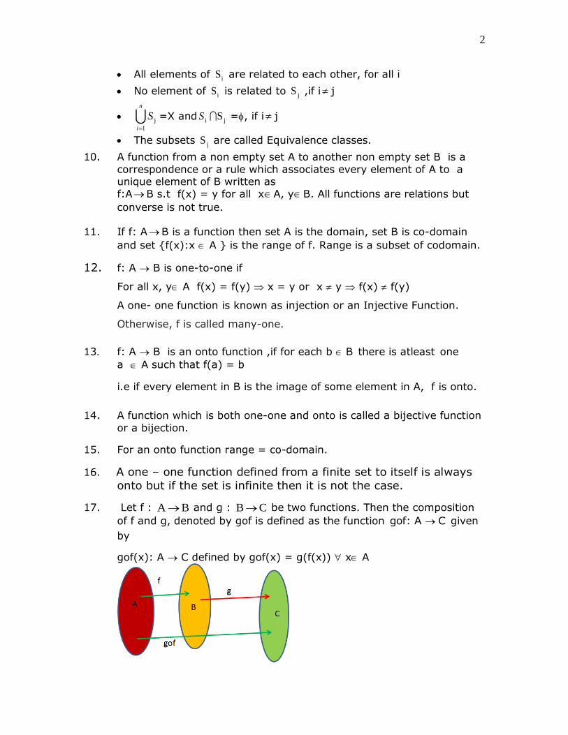
17. Let f : A B and g : B C be two functions. Then the composition

of f and g, denoted by gof is defined as the function gof: A C given

by

gof(x): A C defined by gof(x) = g(f(x)) x A

3

Composition of f and g is written as gof and not fog

gof is defined if the range of f domain of f and fog is defined if

range of g domain of f

18. Composition of functions is not commutative in general

fog(x) ≠ gof(x).Composition is associative

If f: XY, g: YZ and h: ZS are functions then

ho(g o f)=(h o g)of

19. A function f: X Y is defined to be invertible, if there exists a function

g : Y X such that gof = IX and fog = IY. The function g is called the

inverse of f and is denoted by f –1

20. If f is invertible, then f must be one-one and onto and conversely, if fis one- one and onto, then f must be invertible.

21. If f:A B and g: B C are one-one and onto then gof: A C is also

one-one and onto. But If g o f is one –one then only f is one –one g

may or may not be one-one. If g o f is onto then g is onto f may or

may not be onto.

22. Let f: X Y and g: Y Z be two invertible functions. Then gof is also

Invertible with (gof)–1 = f –1o g–1.

23. If f: R R is invertible,

f(x)=y, then 1f (y)=x and (f-1)-1 is the function f itself.

24. A binary operation * on a set A is a function from A X A to A.

25.Addition, subtraction and multiplication are binary operations on R, the

set of real numbers. Division is not binary on R, however, division is a

binary operation on R-{0}, the set of non-zero real numbers

26.A binary operation on the set X is called commutative, if a b=

b a, for every a,bX

27.A binary operation on the set X is called associative, if

a (b*c) =(a*b)*c, for every a, b, cX

28.An element e A is called an identity of A with respect to *, if for

each a A, a * e = a = e * a.

The identity element of (A, *) if it exists, is unique.

4

29.Given a binary operation from A A A, with the identity element e

in A, an element aA is said to be invertible with respect to the operation , if there exists an element b in A such that a b=e= b a,

then b is called the inverse of a and is denoted by a-1.

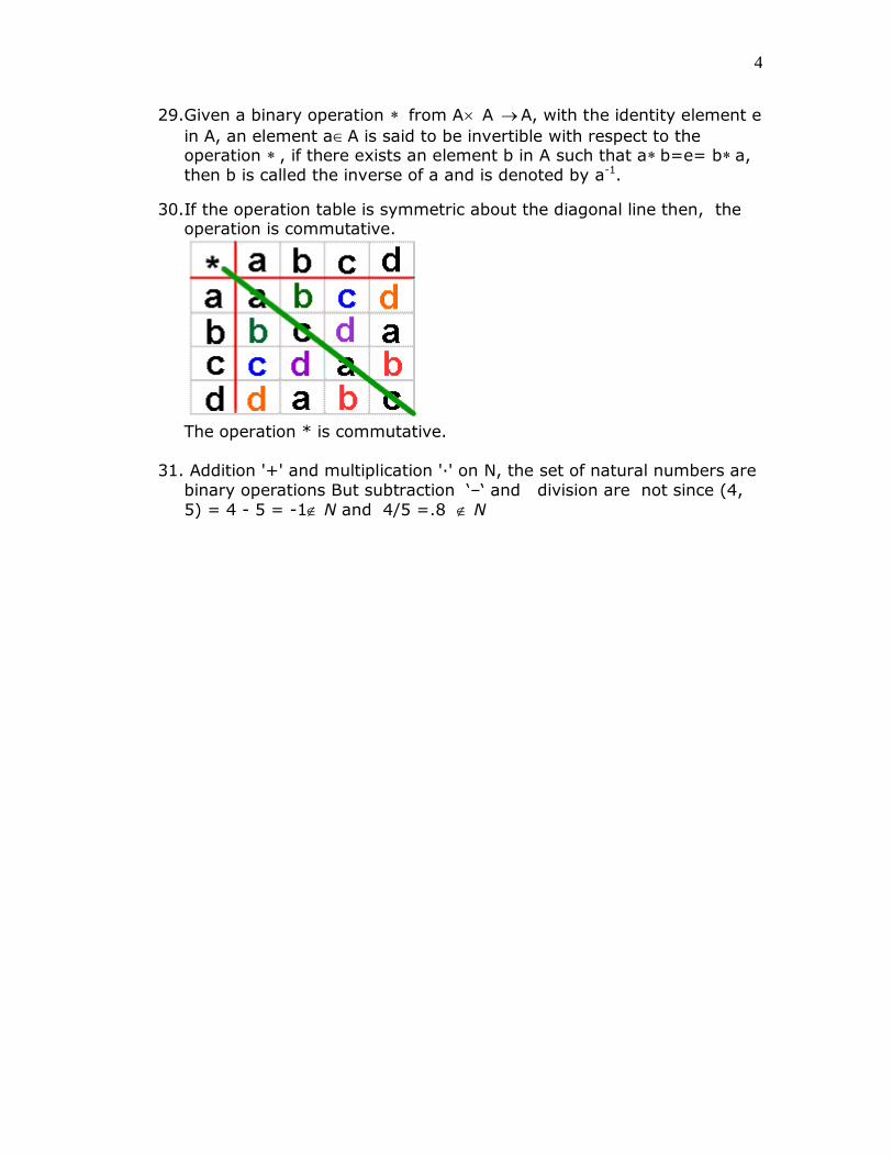
30.If the operation table is symmetric about the diagonal line then, theoperation is commutative.

The operation * is commutative.

31. Addition '+' and multiplication '·' on N, the set of natural numbers are

binary operations But subtraction ‘–‘ and division are not since (4,

5) = 4 - 5 = -1 N and 4/5 =.8 N

1

Class XII

Mathematics

Chapter:2

Inverse Trigonometric Functions

Points to Remember

Key Concepts

1. Inverse trigonometric functions map real numbers back to angles.

2. Inverse of sine function denoted by sin-1 or arc sin(x) is defined on

[-1,1] and range could be any of the intervals

3 3

2 2 2 2 2 2, , , , ,

.

3. The branch of sin-1 function with range2 2

,

is the principal branch.

So sin-1: [-1,1] 2 2

,

4. The graph of sin-1 x is obtained from the graph of sine x by

interchanging the x and y axes

5. Graph of the inverse function is the mirror image (i.e reflection) of the

original function along the line y = x.

6. Inverse of cosine function denoted by cos-1 or arc cos(x) is defined in

[-1,1] and range could be any of the intervals [-,0], [0,],[,2].

So,cos-1: [-1,1] [0,].

2

7. The branch of tan-1 function with range 2 2

,

is the principal

branch. So tan-1: R 2 2

,

.

8. The principal branch of cosec-1 x is2 2

,

-{0}.

cosec-1 x :R-(-1,1) 2 2

,

-{0}.

9. The principal branch of sec-1 x is [0,]-{2

}.

sec-1 x :R-(-1,1) [0,]-{ 2

}.

10. cot-1 is defined as a function with domain R and range as any of the

intervals (-,0), (0,),(,2). The principal branch is (0,)

So cot-1 : R (0,)

11.The value of an inverse trigonometric function which lies in the range

of principal branch is called the principal value of the inverse

trigonometric functions.

12. Inverse of a function is not equal to the reciprocal of the function.

13.Properties of inverse trigonometric functions are valid only on the

principal value branches of corresponding inverse functions or

wherever the functions are defined.

3

Key Formulae

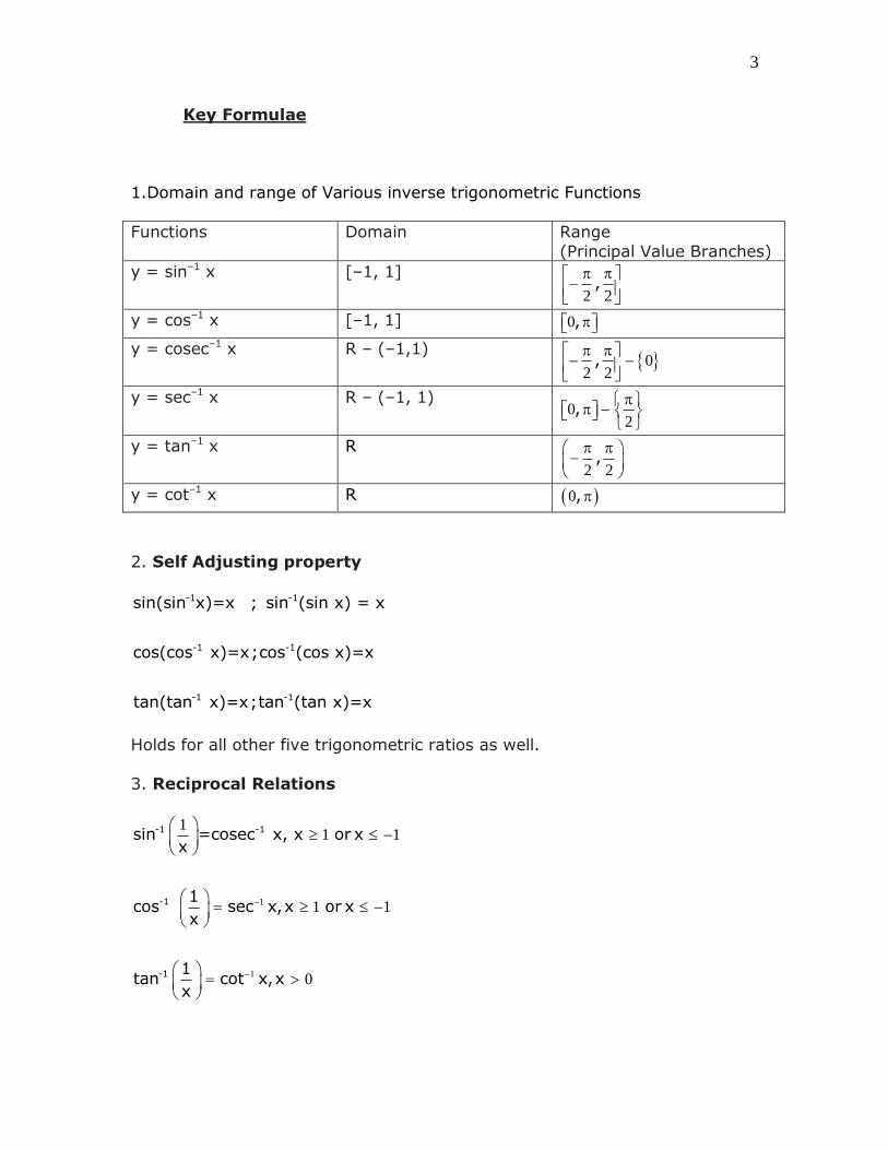
1.Domain and range of Various inverse trigonometric Functions

Functions Domain Range

(Principal Value Branches)

y = sin–1 x [–1, 1]

2 2

,

y = cos–1 x [–1, 1] 0 ,

y = cosec–1 x R – (–1,1) 0

2 2

,

y = sec–1 x R – (–1, 1) 0

2

,

y = tan–1 x R

2 2

,

y = cot–1 x R 0 ,

2. Self Adjusting property

-1 -1

-1 -1

-1 -1

sin(sin x)=x ; sin (sin x) = x

cos(cos x)=x;cos (cos x)=x

tan(tan x)=x;tan (tan x)=x

Holds for all other five trigonometric ratios as well.

3. Reciprocal Relations

1

1

11 1

1 1

0

-1 -1

-1

-1

sin =cosec x, x or xx

1cos sec x,x or x

x

1tan cot x,x

x

4

4. Even and Odd Functions

1

1 1

1 1 1

(i) sin x = -sin x , x -1,1

(ii) tan x = - tan x , x R

(iii) cosec x cosec x, x

1

1 1

1 1

1

1

(iv) cos x cos x,x ,

(v) sec x sec x, x

(vi) cot x cot x,x R

5. Complementary Relations

1 1

1

1 1

1 12

2

12

(i)sin x cos x ,x [ , ]

(ii)tan x cot x ,x R

(iii) cosec x sec x , x

6. Sum and Difference Formuale

1 1 1

1 1 1

11

11

x y(i) tan x tan y tan ,xy

xy

x y(ii)tan x tan y tan ,xy

xy

(iii) sin-1x + sin-1y = 1 2 2sin [x 1 y y 1 x ]

(iv) sin-1x – sin-1y = 1 2 2sin [x 1 y y 1 x ]

(v) cos-1x + cos-1y = 1 2 2cos [xy 1 x 1 y ]

(vi) cos-1x - cos-1y = 1 2 2cos [xy 1 x 1 y ]

(vii) cot-1x + cot-1y = 1 xy 1cot

x y

5

(viii) cot-1x - cot-1y = 1 xy 1cot

y x

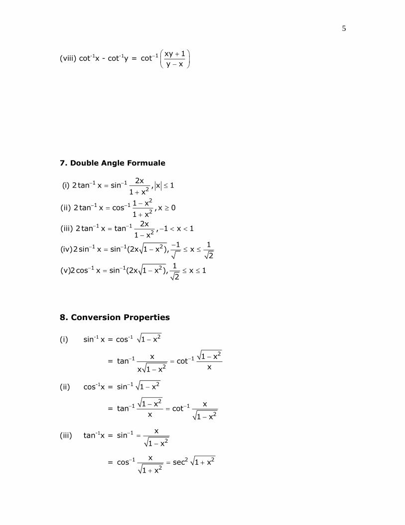
7. Double Angle Formuale

1 1

2

21 1

2

1 1

2

1 1 2

1 1 2

2x(i) 2 tan x sin , x 1

1 x

1 x(ii) 2 tan x cos ,x 0

1 x

2x(iii) 2 tan x tan , 1 x 1

1 x

1 1(iv)2sin x sin (2x 1 x ), x

2

1(v)2cos x sin (2x 1 x ), x 1

2

8. Conversion Properties

(i) sin-1 x = cos-1 21 x

= 2

1 1

2

x 1 xtan cot

xx 1 x

(ii) cos-1x = 1 2sin 1 x

= 2

1 1

2

1 x xtan cot

x 1 x

(iii) tan-1x = 1

2

xsin

1 x

= 1 2 2

2

xcos sec 1 x

1 x

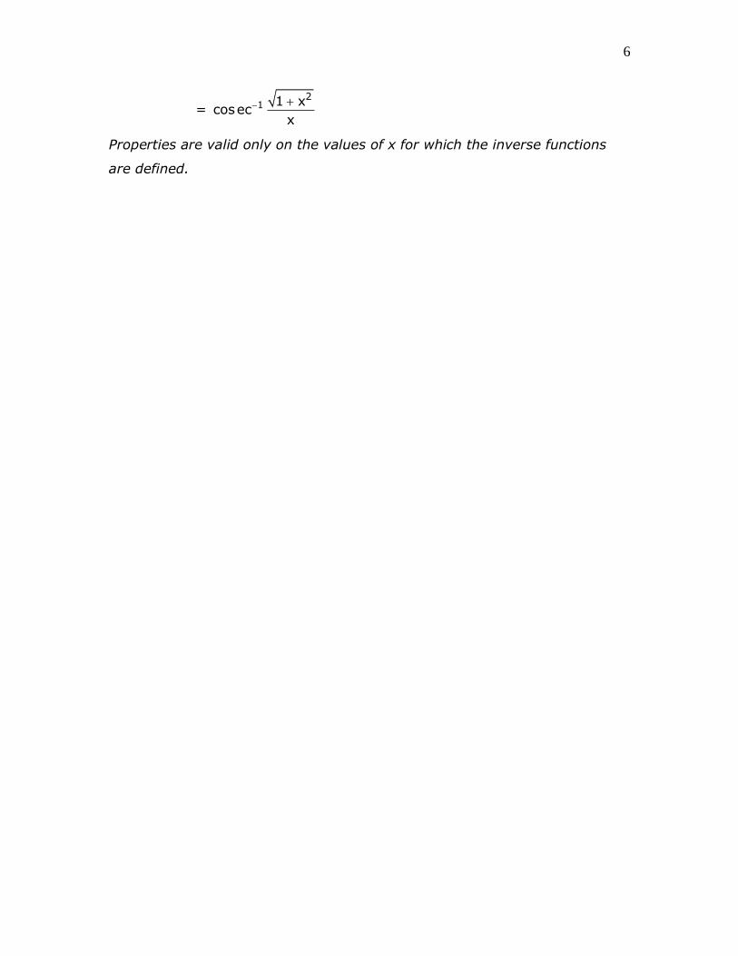
6

= 2

1 1 xcosec

x

Properties are valid only on the values of x for which the inverse functions

are defined.

1

Class XII: Maths

Chapter 3: Matrices

Chapter Notes

Top Definitions

1. Matrix is an ordered rectangular array of numbers (real or complex) or

functions or names or any type of data. The numbers or functions are called

the elements or the entries of the matrix.

2. The horizontal lines of elements are said to constitute, rows of the matrix

and the vertical lines of elements are said to constitute, columns of the

matrix.

3. A matrix is said to be a column matrix if it has only one column.

A = [aij]m x 1 is a column matrix of order m x 1

4. A matrix is said to be a row matrix if it has only one row.

B = [bij]1 x n is a row matrix of order 1 x n.

5. A matrix in which the number of rows is equal to the number of columns is

said to be a square matrix. A matrix of order “m n” is said to be a square

matrix if m = n and is known as a square matrix of order „n‟.

A = [aij]m x n is a square matrix of order m.

6. If A = [aij] is a square matrix of order n, then elements a11, a22, …, ann are

said to constitute the diagonal, of the matrix A

2

7. A square matrix B = [bij]m x m is said to be a diagonal matrix if all its non

diagonal elements are zero, that is a matrix B = [bij]m x m is said to be a

diagonal matrix if bij = 0, when i ≠ j.

8. A diagonal matrix is said to be a scalar matrix if its diagonal elements are

equal, that is, a square matrix B = [bij]n x n is said to be a scalar matrix if

bij = 0, when i ≠ j

bij = k, when i = j, for some constant k.

9. A square matrix in which elements in the diagonal are all 1 and rest are all

zero is called an identity matrix. A square matrix

A = [aij]n x n is an identity matrix, if aij = 1 if i j

0 if i j

10. A matrix is said to be zero matrix or null matrix if all its elements are

zero.

11. Two matrices A = [aij] and B = [bij] are said to be equal if

(i) They are of the same order

(ii) Each elements of A is equal to the corresponding element of B, that is

aij = bij for all i and j.

12. If A = [aij] be an m x n matrix, then the matrix obtained by

interchanging the rows and columns of A is called the transpose of A.

Transpose of the matrix A is denoted by A‟ or (AT).

13. For any square matrix A with real number entries, A + A‟ is a symmetric

matrix and A – A‟ is a skew symmetric matrix.

14. If ij nxnA a is an n n matrix such that AT=A, then A is called

symmetric matrix. In a symmetric matrix, ij jia a for all i and j

15. If ij nxnA a is an n n matrix such that AT=–A, then A is called skew

3

symmetric matrix. In a skew symmetric matrix, ij jia a

If i=j, then ii ii iia a a 0

16. Let A and B be two square matrices of order n such that AB=BA=I.Then A is called inverse of B and is denoted by B=A-1. If B is the inverse of A

, then A is also the inverse of B.

17. If A and B are two invertible matrices of same order, then (AB)-1 = B-1 A-1

Top Concepts

1. Order of a matrix gives the number of rows and columns present in the

matrix.

2. If the matrix A has m rows and n columns then it is denoted by

A =[aij]m x n . ija is i-j th or (i, j)th element of the matrix.

3. The simplest classification of matrices is based on the order of the matrix.

4. In case of a square matrix, the collection of elements a11 , a22, and so on

constitute the Principal Diagonal or simply the diagonal of the matrix Diagonal is defined only in case of square matrices.

5. Two matrices of same order are comparable matrices.

6. Ifij ijm xn m xn

A a and B b are two matrices of order m × n, their sum is

defined as a matrix ij m xnC c

where

ij ij ijc a b for 1 i m,1 j n

4

7.Two matrices can be added9or subtracted) if they are of same order. For

multiplying two matrices A and B number of columns in A must be equal to the number of rows in B.

8. ij m x nA a is a matrix and k is a scalar, then kA is another matrix which

is obtained by multiplying each element of A by the scalar k. Hence

ij m xnkA ka

9. If ij ijm xn m xnA a and B b are two matrices, their difference is

represented as A B A ( 1)B .

10. Properties of matrix addition

(i) Matrix addition is commutative i.e A+B = B+A.

(ii) Matrix addition is associative i.e (A + B) + C = A + (B + C).

(iii) Existence of additive identity: Null matrix is the identity w.r.t addition

of matrices

Given a matrix ij m x nA a , there will be a corresponding null matrix O of

same order such that A+O=O+A=A

(iv) The existence of additive inverse Let A = [aij]m x n be any matrix, then

there exists another matrix –A = -[aij]m x n such that

A + (–A) = (–A) + A = O.

11. Properties of scalar multiplication of the matrices:

If ij ijA a ,B b are two matrices, and k,L are real numbers then

(i) k(A +B) = k A + kB, (ii) (k + I)A = k A + I A

(ii) k (A + B) = k([aij]+[bij]) = k[aij]+k[bij ] = kA+kB

(iii) ij ij(k L)A (k L) a (k L)a = k [aij ] + L [aij ] = k A + L A

12. If ij ijmxp pxnA a ,B b are two matrices, their product AB, is given by

ij mxnC c such that

p

ij ik kj i j i j i j ip pjk

c a b a b a b a b ... a b

1 1 2 2 3 31

.

5

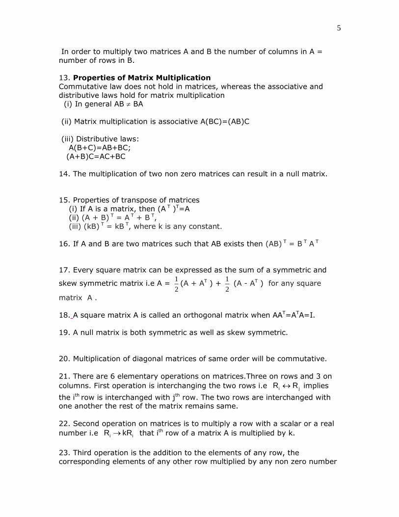
In order to multiply two matrices A and B the number of columns in A =

number of rows in B.

13. Properties of Matrix Multiplication

Commutative law does not hold in matrices, whereas the associative and

distributive laws hold for matrix multiplication (i) In general AB BA

(ii) Matrix multiplication is associative A(BC)=(AB)C

(iii) Distributive laws:

A(B+C)=AB+BC;

(A+B)C=AC+BC

14. The multiplication of two non zero matrices can result in a null matrix.

15. Properties of transpose of matrices

(i) If A is a matrix, then (A T )T=A

(ii) (A + B) T = A T + B T,

(iii) (kB) T = kB T, where k is any constant.

16. If A and B are two matrices such that AB exists then (AB) T = B T A T

17. Every square matrix can be expressed as the sum of a symmetric and

skew symmetric matrix i.e A = 1

2(A + AT ) +

1

2 (A - AT ) for any square

matrix A .

18. A square matrix A is called an orthogonal matrix when AAT=ATA=I.

19. A null matrix is both symmetric as well as skew symmetric.

20. Multiplication of diagonal matrices of same order will be commutative.

21. There are 6 elementary operations on matrices.Three on rows and 3 on

columns. First operation is interchanging the two rows i.e i jR R implies

the ith row is interchanged with jth row. The two rows are interchanged with one another the rest of the matrix remains same.

22. Second operation on matrices is to multiply a row with a scalar or a real

number i.e i iR kR that ith row of a matrix A is multiplied by k.

23. Third operation is the addition to the elements of any row, the

corresponding elements of any other row multiplied by any non zero number

6

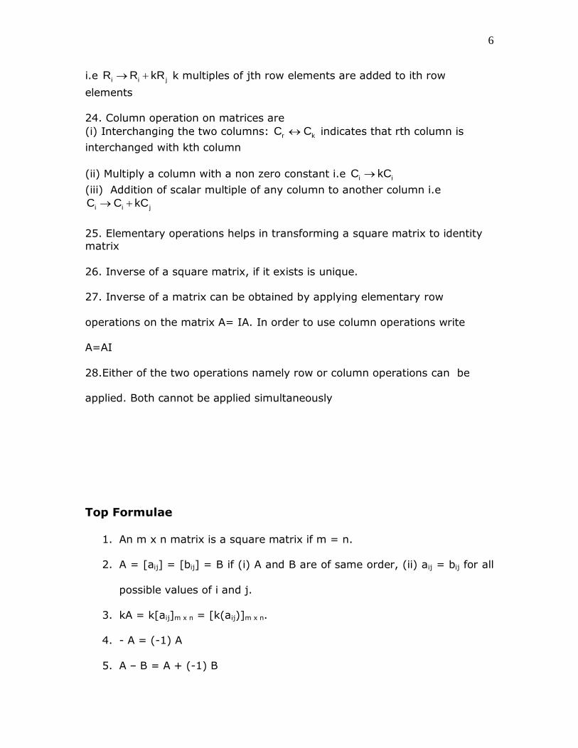
i.e i i jR R kR k multiples of jth row elements are added to ith row

elements

24. Column operation on matrices are

(i) Interchanging the two columns: r kC C indicates that rth column is

interchanged with kth column

(ii) Multiply a column with a non zero constant i.e i iC kC

(iii) Addition of scalar multiple of any column to another column i.e

i i jC C kC

25. Elementary operations helps in transforming a square matrix to identity

matrix

26. Inverse of a square matrix, if it exists is unique.

27. Inverse of a matrix can be obtained by applying elementary row

operations on the matrix A= IA. In order to use column operations write

A=AI

28.Either of the two operations namely row or column operations can be

applied. Both cannot be applied simultaneously

Top Formulae

1. An m x n matrix is a square matrix if m = n.

2. A = [aij] = [bij] = B if (i) A and B are of same order, (ii) aij = bij for all

possible values of i and j.

3. kA = k[aij]m x n = [k(aij)]m x n.

4. - A = (-1) A

5. A – B = A + (-1) B

7

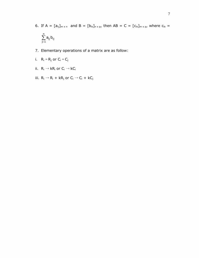
6. If A = [aij]m x n and B = [bik]n x p, then AB = C = [cik]m x p, where cik =

n

ij ijj 1

a b

7. Elementary operations of a matrix are as follow:

i. Ri ↔ Rj or Ci ↔ Cj

ii. Ri → kRi or Ci → kCi

iii. Ri → Ri + kRj or Ci → Ci + kCj

1

Class XII: Mathematics

Chapter 4: Determinants

Chapter Notes

Top Definitions

1. To every square matrix A =[aij] a unique number (real or complex)

called determinant of the square matrix A can be associated.

Determinant of matrix A is denoted by det(A) or |A| or .

2. A determinant can be thought of as a function which associates each

square matrix to a unique number (real or complex).

f:M K is defined by f(A) = k where A M the set of square

matrices and k K set of numbers(real or complex)

3. Let A = [a] be the matrix of order 1, then determinant of A is defined

to be equal to a.

4. Determinant of order 2

11 12 11 12

11 22 12 21

21 22 21 22

a a a aIf A then, A a a a a

a a a a

5. Determinant of order 3

If 11 12 13

21 22 23

31 32 33

a a a

A a a a

a a a

then

|A|=11 12 13

21 22 23

31 32 33

a a a

a a a

a a a

22 23 21 23 21 22

11 12 13

32 33 31 33 31 32

a a a a a aa a a

a a a a a a

6. Minor of an element aij of a determinant is the determinant obtained

by deleting its ith row and jth column in which element aij lies. Minor of

an element aij is denoted by Mij.

2

7. Cofactor of an element aij, denoted by Aij is defined by

Aij = (-1)i+j.Mij where Mij is the minor of aij.

8. The adjoint of a square matrix A=[aij] is the transpose of the cofactor

matrix [Aij]nn.

9. A square matrix A is said to be singular if |A| = 0

10.A square matrix A is said to be non – singular if |A|≠ 0

11.If A and B are nonsingular matrices of the same order, then AB and BA

are also nonsingular matrices of the same order.

12.The determinant of the product of matrices is equal t product of the

respective determinants, that is, |AB| = |A| |B|, where A and B are

square matrices of the same order.

13. A square matrix A is invertible i.e its inverse exists if and only if A is

nonsingular matrix. Inverse of matrix A if exists is given by

A-1 = 1

(adjA)A

14.A system of equations is said to be consistent if its solution (one or

more) exists.

15.A system of equations is said to be inconsistent if its solution does not

exist.

Top Concepts

1. A determinant can be expanded along any of its row (or column). For

easier calculations it must be expanded along the row (or column)

containing maximum zeros.

3

2. If A=kB where A and B are square matrices of order n, then |A|=kn |B|

where n =1,2,3.

Properties of Determinants

3. Property 1 Value of the determinant remains unchanged if its row

and columns are interchanged. If A is a square matrix, the

det (A) = det (A’), where A’ = transpose of A.

4. Property 2 If two rows or columns of a determinant are interchanged,

then the sign of the determinant is changed. Interchange of rows and

columns is written as Ri Rj or Ci Cj

5. Property 3: If any two rows (or columns) of a determinant are

identical, then value of determinant is zero.

6. Property 4: If each element of a row (or a column) of a determinant

is multiplied by a constant k, then its value get multiplied by k.

If Δ1 is the determinant obtained by applying Ri → kRi or Ci → kCi to

the determinant Δ, then Δ1 = kΔ. So .if A is a square matrix of order n

and k is a scalar, then |kA|=kn|A|. This property enables taking out of

common factors from a given row or column.

7. Property 5: If in a determinant, the elements in two rows or columns

are proportional, then the value of the determinant is zero. For

example.

1 2 3

1 2 3

1 2 3

a a a

b b b 0

ka ka ka

(rows R1 and R3 are proportional)

4

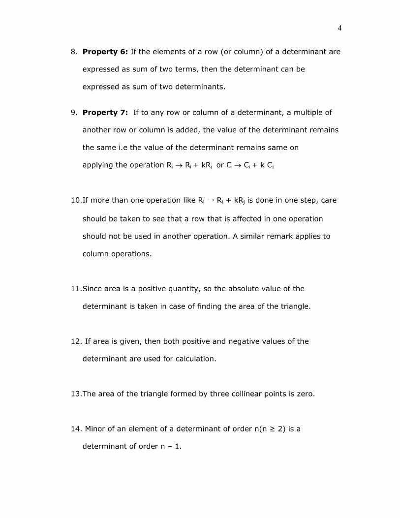
8. Property 6: If the elements of a row (or column) of a determinant are

expressed as sum of two terms, then the determinant can be

expressed as sum of two determinants.

9. Property 7: If to any row or column of a determinant, a multiple of

another row or column is added, the value of the determinant remains

the same i.e the value of the determinant remains same on

applying the operation Ri Ri + kRj or Ci Ci + k Cj

10.If more than one operation like Ri → Ri + kRj is done in one step, care

should be taken to see that a row that is affected in one operation

should not be used in another operation. A similar remark applies to

column operations.

11.Since area is a positive quantity, so the absolute value of the

determinant is taken in case of finding the area of the triangle.

12. If area is given, then both positive and negative values of the

determinant are used for calculation.

13.The area of the triangle formed by three collinear points is zero.

14. Minor of an element of a determinant of order n(n ≥ 2) is a

determinant of order n – 1.

5

15.Value of determinant of a matrix A is obtained by sum of product of

elements of a row (or a column) with corresponding cofactors. For

example |A|= a11A11+a12A12+a13A13

16.If elements of a row (or column) are multiplied with cofactors of any

other row (or column), then their sum is zero. For example

a11A21+a12A22+a13A23 = 0

17.If A is a nonsingular matrix of order n then |adj.A|=|A|n-1

18.Determinants can be used to find the area of triangles if its vertices

are given

19.Determinants and matrices can also be used to solve the system of

linear equations in two or three variables.

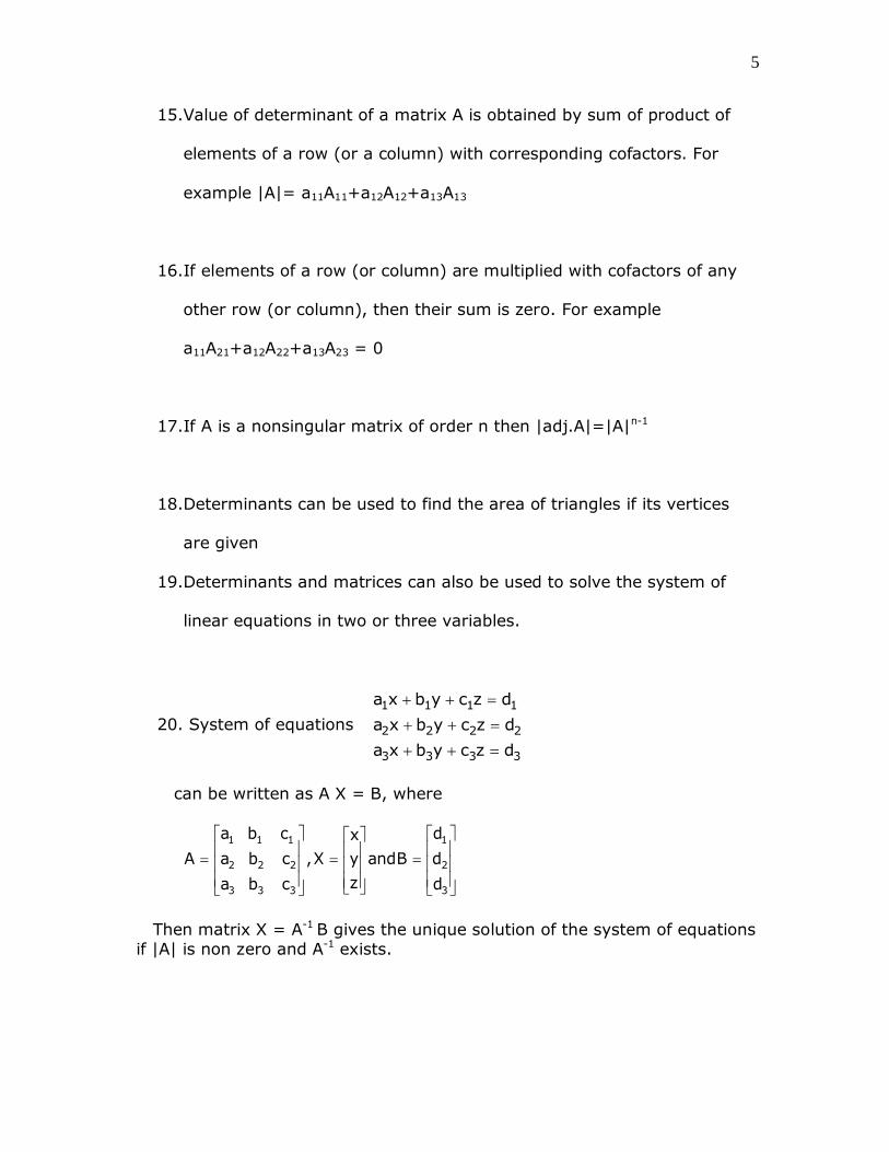
20. System of equations

1 1 1 1

2 2 2 2

3 3 3 3

a x b y c z d

a x b y c z d

a x b y c z d

can be written as A X = B, where

1 1 1 1

2 2 2 2

3 3 3 3

a b c dx

A a b c ,X y andB d

za b c d

Then matrix X = A-1 B gives the unique solution of the system of equations

if |A| is non zero and A-1 exists.

6

Top Formulae

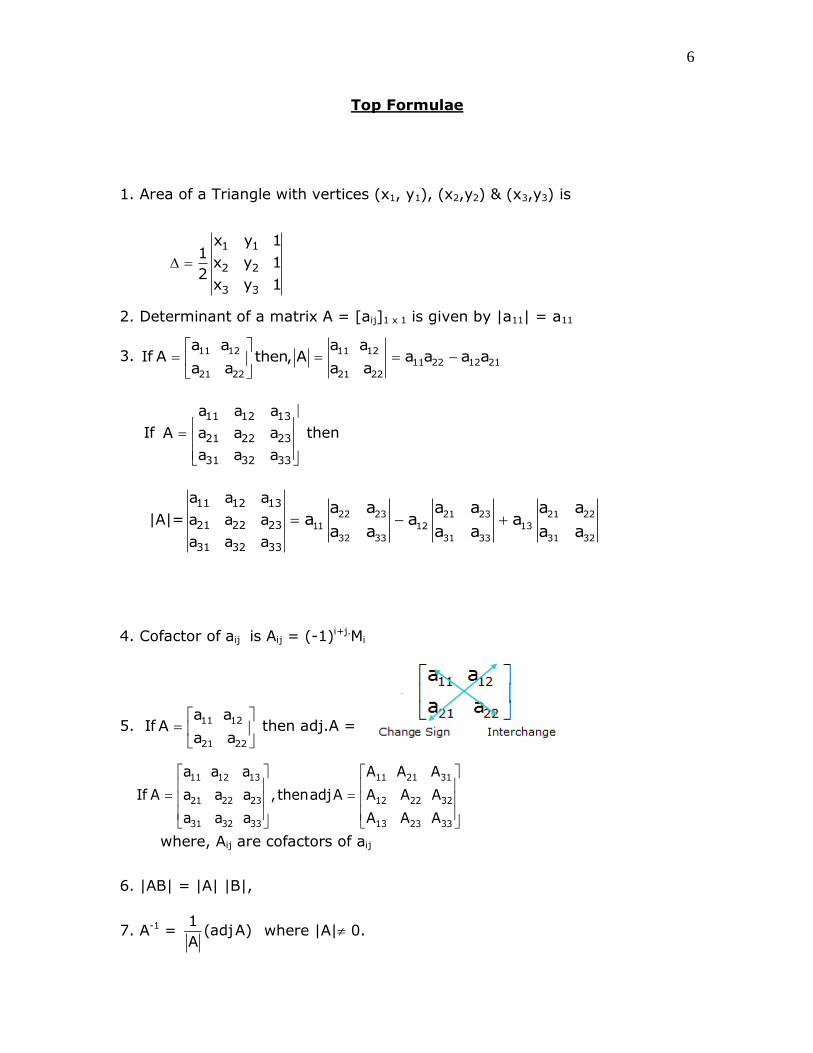
1. Area of a Triangle with vertices (x1, y1), (x2,y2) & (x3,y3) is

1 1

2 2

3 3

x y 11

x y 12

x y 1

2. Determinant of a matrix A = [aij]1 x 1 is given by |a11| = a11

3. 11 12 11 12

11 22 12 21

21 22 21 22

a a a aIf A then, A a a a a

a a a a

If 11 12 13

21 22 23

31 32 33

a a a

A a a a

a a a

then

|A|=11 12 13

21 22 23

31 32 33

a a a

a a a

a a a

22 23 21 23 21 22

11 12 13

32 33 31 33 31 32

a a a a a aa a a

a a a a a a

4. Cofactor of aij is Aij = (-1)i+j.Mi

5. If

11 12

21 22

a aA

a a then adj.A =

11 12 13 11 21 31

21 22 23 12 22 32

31 32 33 13 23 33

a a a A A A

If A a a a ,thenadjA A A A

a a a A A A

where, Aij are cofactors of aij

6. |AB| = |A| |B|,

7. A-1 =1

(adjA)A

where |A| 0.

7

8. |A-1| =1

| A | and (A-1)-1 = A

9. Unique solution of equation AX = B is given by X = A-1B, where |A|≠ 0.

10. For a square matrix A in matrix equation AX = B,

i. |A|≠ 0, there exists unique solution.

ii. |A|= 0 and (adj A) B ≠ 0, then there exists no solution.

iii. |A| = 0, and (adj A) B = 0, then system may or may not be consistent.

1

Class XII

Mathematics

Chapter:5

Continuity and Differentiability

Chapter Notes

Key Definitions

1. A function f(x) is said to be continuous at a point c if,

x c x c

lim f(x) lim f(x) f(c)

2. A real function f is said to be continuous if it is continuous at every

point in the domain of f.

3. If f and g are real valued functions such that (f o g) is defined at c.

If g is continuous at c and if f is continuous at g(c), then (f o g) is

continuous at c.

4. A function f is differentiable at a point c if LHD=RHD

i.eh 0 h 0

f(c h) f(c) f(c h) f(c)lim lim

h h

5. Chain Rule of Differentiation: If f is a composite function of two

functions u and v such that f = vou and t =u(x)

if both dt dv

anddx dx

, exists then, df dv dt

.dx dt dx

6. Logarithm of a to base b is xi.e logb a =x if bx = a where b > 1 be

a real number. Logarithm of a to base b is denoted by logb a.

7. Functions of the form x = f(t) and y = g(t) are parametric

functions.

8. Rolle’s Theorem: If f : [a, b] R is continuous on [a, b] and

differentiable on (a, b) such that f (a) = f (b), then there exists

some c in (a, b) such that f’(c) = 0

2

9. Mean Value Theorem: If f :[a, b] R is continuous on [a, b] &

differentiable on (a, b). Then there exists some c in (a, b) such that

'

h 0

f(b) f(a)f (c) lim

b a

Key Concepts

1. A function is continuous at x = c if the function is defined at x = c and

the value of the function at x = c equals the limit of the function at x =

c.

2. If function f is not continuous at c, then f is discontinuous at c and c is

called the point of discontinuity of f.

3. Every polynomial function is continuous.

4. Greatest integer function, [x] is not continuous at the integral values

of x.

5. Every rational function is continuous.

6. Algebra of Continuous Functions

Let f and g be two real functions continuous at a real number c, then

(1) f + g is continuous at x = c

(2) f – g is continuous at x = c

(3) f. g is continuous at x = c

(4) f

g

is continuous at x = c, (provided g(c) ≠ 0).

7. Derivative of a function f with respect to x is f’(x) which is given by

'

h 0

f(x h) f(x)f (x) lim

h

8. If a function f is differentiable at a point c, then it is also continuous at

that point.

9. Every differentiable function is continuous but converse is not true.

10.Chain Rule is used to differentiate composites of functions.

11. Algebra of Derivatives:

3

If u & v are two functions which are differentiable, then

(i) (u v)' u' v' (Sum and DifferenceFormula)

(ii) (uv)' u'v uv' (Product rule)

(iii)

'

2

u u'v uv'(Quotient rule)

v v

12.Implicit Functions

If it is not possible to “separate” the variables x & y then function f is

known as implicit function.

13.Exponential function: A function of the form y = f (x) = bx where

base b > 1

(1) Domain of the exponential function is R, the set of all real numbers.

(2) The point (0, 1) is always on the graph of the exponential function

(3) Exponential function is ever increasing

14.Properties of Logarithmic functions

(i)Domain of log function is R+.

(ii) The log function is ever increasing

(iii) For x very near to zero, the value of log x can be made lesser than

any given real number.

15.Logarithmic differentiation is a powerful technique to differentiate

functions of the form f(x) = [u (x)]v(x). Here both f(x) and u(x) need to

be positive.

16.Logarithmic Differentiation

y=ax

Taking logarithm on both sides

log log xy a .

Using property of logarithms

log logy x a

Now differentiating the implicit function 1 dy

. logay dx

xdyyloga a loga

dx

.

4

17. A relation between variables x and y expressed in the form x=f(t)

and y=g(t) is the parametric form with t as the parameter .Parametric

equation of parabola y2=4ax is x=at2,y=2at

18.Parametric Differentiation:

Differentiation of the functions of the form x = f(t) and y = g(t)

dydy dt

dxdx

dt

dy dy dt

dx dt dx

19.If y =f(x) anddy

dx=f’(x) and if f’(x) is differentiable then

2

2

d dy d y

dx dx dxor f’’ (x) is the second order derivative of y w.r.t x

Top Formulae

1. Derivative of a function at a point

'

h 0

f(x h) f(x)f (x) lim

h

2. Properties of Logarithms

y

log xy logx logy

xlog logx logy

y

log x ylogx

ab

b

log xlog x

log a

3.Derivatives of Functions

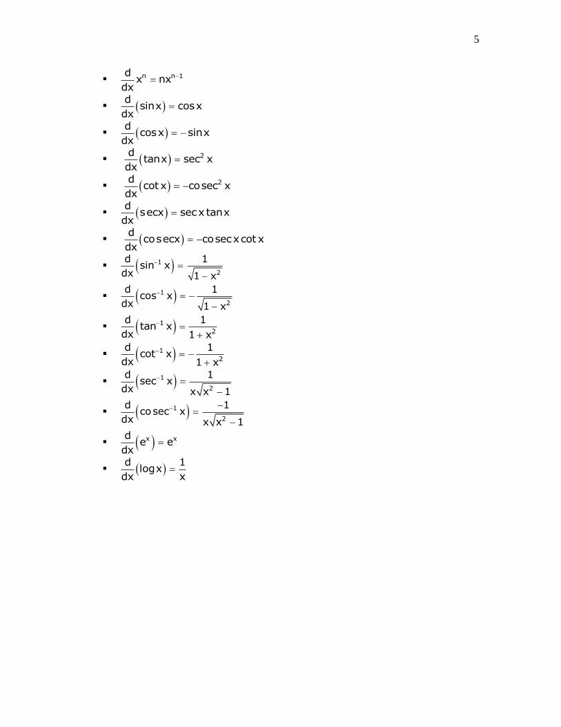
5

n n 1d

x nxdx

d

sinx cosxdx

d

cosx sinxdx

2dtanx sec x

dx

2dcotx cosec x

dx

d

secx secx tanxdx

d

cosecx cosecxcot xdx

1

2

d 1sin x

dx 1 x

1

2

d 1cos x

dx 1 x

1

2

d 1tan x

dx 1 x

1

2

d 1cot x

dx 1 x

1

2

d 1sec x

dx x x 1

1

2

d 1cosec x

dx x x 1

x xde e

dx

d 1

logxdx x

1

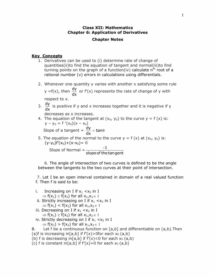
Class XII: Mathematics

Chapter 6: Application of Derivatives

Chapter Notes

Key Concepts

1. Derivatives can be used to (i) determine rate of change of

quantities(ii)to find the equation of tangent and normal(iii)to find turning points on the graph of a function(iv) calculate nth root of a

rational number (v) errors in calculations using differentials.

2. Whenever one quantity y varies with another x satisfying some rule

y =f(x), then dy

dx or f’(x) represents the rate of change of y with

respect to x.

3. dy

dx is positive if y and x increases together and it is negative if y

decreases as x increases. 4. The equation of the tangent at (x0, y0) to the curve y = f (x) is:

y – y0 = f ′(x0)(x – x0)

Slope of a tangent = dy

tandx

5. The equation of the normal to the curve y = f (x) at (x0, y0) is:

(y-y0)f’(x0)+(x-x0)= 0

Slope of Normal =1

slopeof thetangent

6. The angle of intersection of two curves is defined to be the anglebetween the tangents to the two curves at their point of intersection.

7. Let I be an open interval contained in domain of a real valued function

f. Then f is said to be:

i. Increasing on I if x1 <x2 in I

f(x1) f(x2) for all x1,x2

ii. Strictly increasing on I if x1 <x2 in I f(x1) < f(x2) for all x1,x2

iii. Decreasing on I if x1 <x2 in I f(x1) f(x2) for all x1,x2

iv. Strictly decreasing on I if x1 <x2 in I

f(x1) > f(x2) for all x1,x2

8.Let f be a continuous function on [a,b] and differentiable on (a,b).Then

(a)f is increasing in[a,b] if f’(x)>0for each x(a,b)

(b) f is decreasing in[a,b] if f’(x)<0 for each x(a,b)

(c) f is constant in[a,b] if f’(x)=0 for each x(a,b)

2

9. Let f be a continuous function on [a,b] and differentiable on (a,b).Then

(a) f is strictly increasing in (a,b) if f’(x)>0for each x(a,b)

(b) f is strictly decreasing in (a,b) if f’(x)<0 for each x(a,b)

(c) f is constant in (a,b) if f’(x)=0 for each x(a,b)

10. A function which is either increasing or decreasing is called a monotonic

function

11. Let f be a function defined on I.Then

a f is said to have a maximum value in I, if there exists a point c in I such

that f (c) > f (x), for all x I.

The number f (c) is called the maximum value of f in I and the point c

is called a point of maximum value of f in I.

b. f is said to have a minimum value in I, if there exists a point c in I

such that f (c) < f (x), for all x I.

The number f (c), in this case, is called the minimum value of f in I

and the point c, in this case, is called a point of minimum value of f in

I.

c. f is said to have an extreme value in I if there exists a point c in I such

that f (c) is either a maximum value or a minimum value of f in I.

The number f (c) , in this case, is called an extreme value of f in I and

the point c, is called an extreme point.

12. Every monotonic function assumes its maximum/ minimum value at the

end points of the domain of definition of the function.

13. Every continuous function on a closed interval has a maximum and a

minimum value

14. Derivative of a function at the point c represents the slope of tangent to

the given curve at a point x=c.

15.If f’(c)=0 i.e. derivative at a point x=c vanishes, which means slope ofthe tangent at x=c is zero. Geometrically, this will imply that this tangent is

parallel to x axis so x=c will come out to be a turning point of the curve.

Such points where graph takes a turn are called extreme points.

16.Let f be a real valued function and let c be an interior point in the domain

of f. Then

a. c is called a point of local maxima if there is h > 0 such that

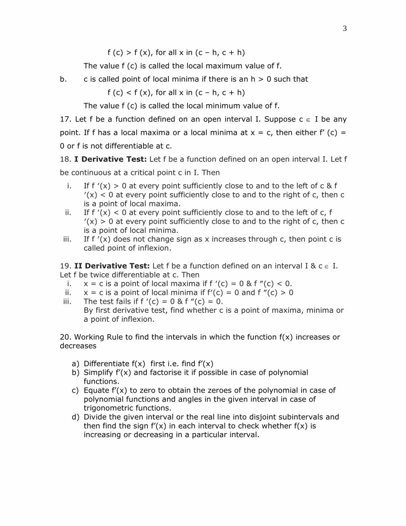
3

f (c) > f (x), for all x in (c – h, c + h)

The value f (c) is called the local maximum value of f.

b. c is called point of local minima if there is an h > 0 such that

f (c) < f (x), for all x in (c – h, c + h)

The value f (c) is called the local minimum value of f.

17. Let f be a function defined on an open interval I. Suppose c I be any

point. If f has a local maxima or a local minima at x = c, then either f’ (c) =

0 or f is not differentiable at c.

18. I Derivative Test: Let f be a function defined on an open interval I. Let f

be continuous at a critical point c in I. Then

i. If f ′(x) > 0 at every point sufficiently close to and to the left of c & f

′(x) < 0 at every point sufficiently close to and to the right of c, then c

is a point of local maxima. ii. If f ′(x) < 0 at every point sufficiently close to and to the left of c, f

′(x) > 0 at every point sufficiently close to and to the right of c, then c

is a point of local minima. iii. If f ′(x) does not change sign as x increases through c, then point c is

called point of inflexion.

19. II Derivative Test: Let f be a function defined on an interval I & c I.

Let f be twice differentiable at c. Then i. x = c is a point of local maxima if f ′(c) = 0 & f ″(c) < 0.

ii. x = c is a point of local minima if f′(c) = 0 and f ″(c) > 0

iii. The test fails if f ′(c) = 0 & f ″(c) = 0.By first derivative test, find whether c is a point of maxima, minima or

a point of inflexion.

20. Working Rule to find the intervals in which the function f(x) increases ordecreases

a) Differentiate f(x) first i.e. find f’(x)b) Simplify f’(x) and factorise it if possible in case of polynomial

functions.

c) Equate f’(x) to zero to obtain the zeroes of the polynomial in case of

polynomial functions and angles in the given interval in case of trigonometric functions.

d) Divide the given interval or the real line into disjoint subintervals and

then find the sign f’(x) in each interval to check whether f(x) is increasing or decreasing in a particular interval.

4

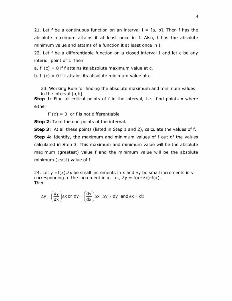
21. Let f be a continuous function on an interval I = [a, b]. Then f has the

absolute maximum attains it at least once in I. Also, f has the absolute

minimum value and attains of a function it at least once in I.

22. Let f be a differentiable function on a closed interval I and let c be any

interior point of I. Then

a. f’ (c) = 0 if f attains its absolute maximum value at c.

b. f’ (c) = 0 if f attains its absolute minimum value at c.

23. Working Rule for finding the absolute maximum and minimum values

in the interval [a,b]

Step 1: Find all critical points of f in the interval, i.e., find points x where

either

f’ (x) = 0 or f is not differentiable

Step 2: Take the end points of the interval.

Step 3: At all these points (listed in Step 1 and 2), calculate the values of f.

Step 4: Identify, the maximum and minimum values of f out of the values

calculated in Step 3. This maximum and minimum value will be the absolute

maximum (greatest) value f and the minimum value will be the absolute

minimum (least) value of f.

24. Let y =f(x),x be small increments in x and y be small increments in y

corresponding to the increment in x, i.e., y = f(x+x)-f(x).

Then

dy

y xdx

or

dydy x

dx

y dy and x dx

1

Class XII: Mathematics

Chapter 7: Integrals

Chapter Notes

Key Concepts

1. Integration is the inverse process of differentiation. The process of

finding the function from its primitive is known as integration or anti differentiation.

2. Indefinite Integral f(x)dx F(x) C where F(x) is the antiderivative

of f(x).

3. f(x)dx means integral of f w.r.t x ,f(x) is the integrand, x is the

variable of integration, C is the constant of integration.

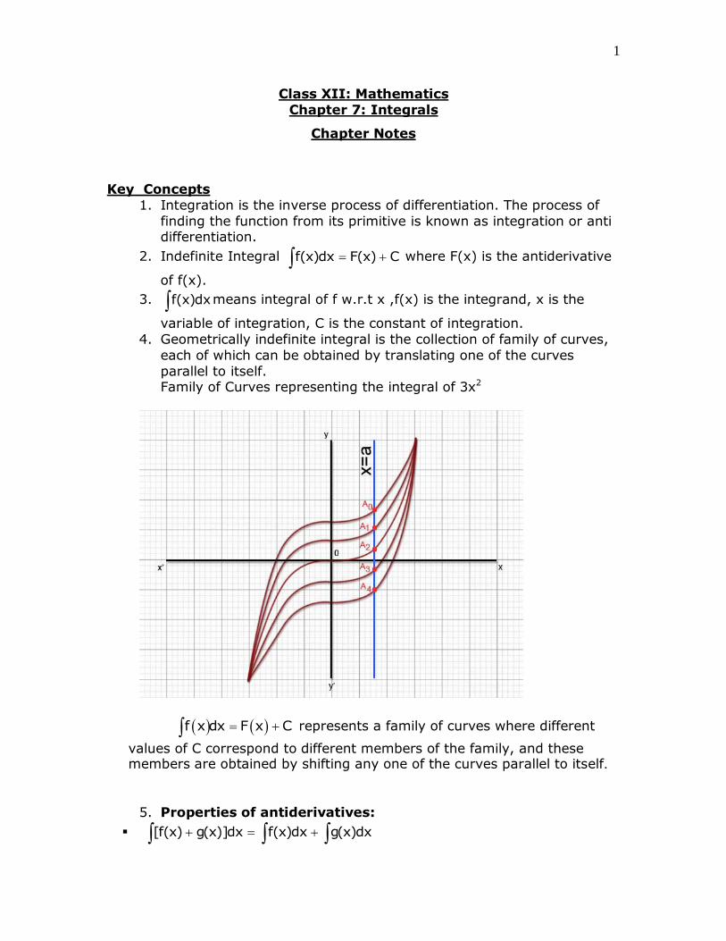
4. Geometrically indefinite integral is the collection of family of curves,

each of which can be obtained by translating one of the curves

parallel to itself. Family of Curves representing the integral of 3x2

f x dx F x C represents a family of curves where different

values of C correspond to different members of the family, and these members are obtained by shifting any one of the curves parallel to itself.

5. Properties of antiderivatives:

[f(x) g(x)]dx f(x)dx g(x)dx

2

kf(x)dx k f(x)dx for any real number k

1 1 2 2 n n 1 1 2 2 n n[k f (x) k f (x) ...... k f (x)]dx k f (x)dx k f (x)dx .... k f (x)dx where, k1,k2…kn are real numbers & f1,f2,..fn are real functions

6.By knowing one anti-derivative of function f infinite number of anti

derivatives can be obtained.

7.Integration can be done using many methods prominent among them are(i)Integration by substitution

(ii)Integration using Partial Fractions

(iii)Integration by Parts (iv) Integration using trigonometric identities

8. A change in the variable of integration often reduces an integral to one of

the fundamental integrals. Some standard substitutions are

x2+a2 substitute x = a tan

2 2x -a substitute x = a sec

2 2a x substitute x = a sin or a cos

9. A function of the formP(x)

Q(x) is known as rational function. Rational

functions can be integrated using Partial fractions.

10. Partial fraction decomposition or partial fraction expansion is used

to reduce the degree of either the numerator or the denominator of a rational function.

11. Integration using Partial Fractions

A rational functionP(x)

Q(x) can be expressed as sum of partial fractions if

P(x)

Q(x)

this takes any of the forms.

px q A B

(x a)(x b) x a x b

, a≠b

2 2

px q A B

x a(x a) (x a)

2px qx r A B C

(x a)(x b)(x c) x a x b x c

2

2 2

px qx r A B C

x a x b(x a) (x b) (x a)

2

2 2

px qx r A Bx C

x a(x a)(x bx c) x bx c

3

where 2x bx c cannot be factorised further.

12.To find the integral of the function2

dx

ax bx c or2

dx

ax bx c

ax2+bx+c must be expressed as

2 2

2

b c ba x

2a a 4a

13. To find the integral of the function2

(px q)dx

ax bx c

or2

(px q)dx

ax bx c

; px+q

= A. d

dx(ax2+bx+c)+B =A(2ax+b)+B

14.To find the integral of the product of two functions integration by parts is

used.I and II functions are chosen using ILATE rule

I- inverse trigonometric

L- logarithmic A-algebra T-Trigonometric E-exponential , is used to identify the first function

14. Integration by parts:

The integral of the product of two functions = (first function) × (integral of

the second function) – Integral of [(differential coefficient of the first function)× (integral of the second function)]

1 2 1 2 1 2

df (x).f (x)dx f (x) f (x)dx f (x). f (x)dx dx

dx

where f1 & f2 are functions

of x.

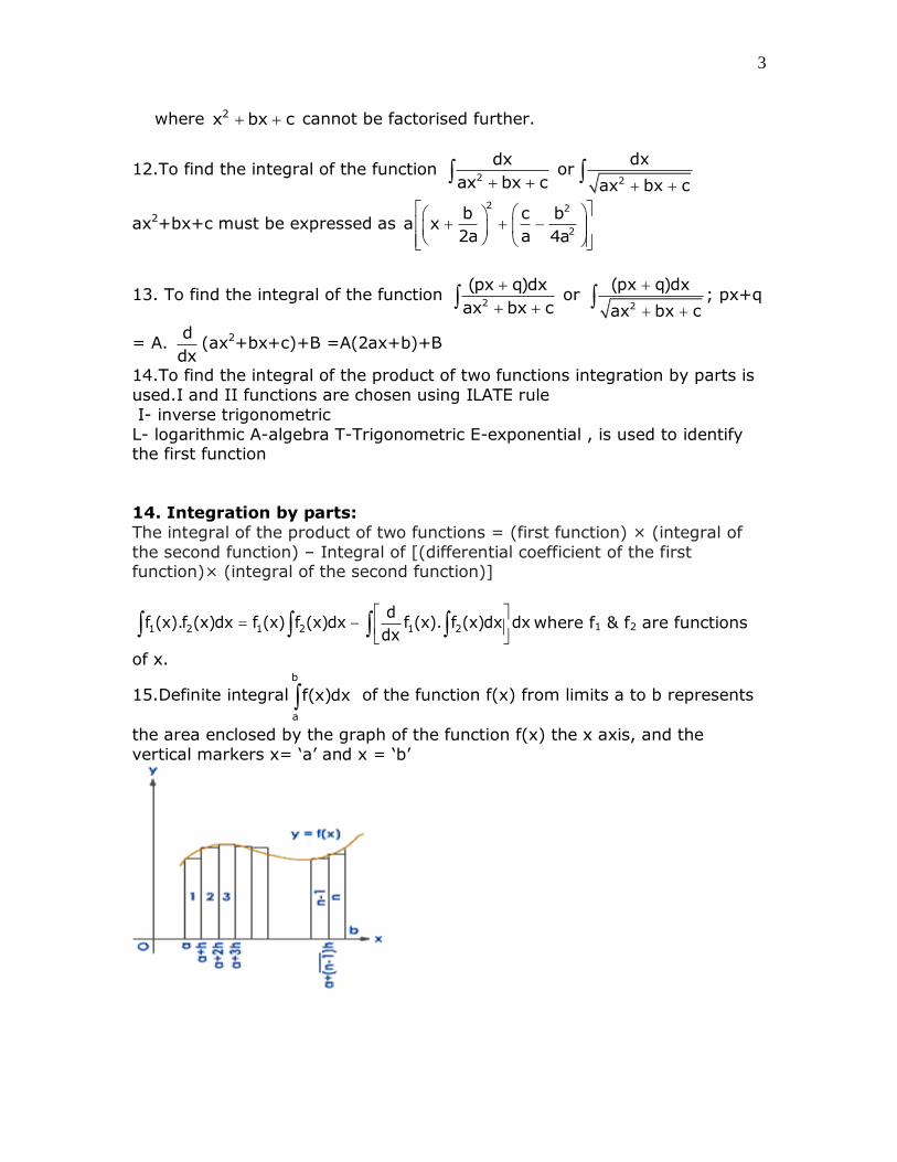
15.Definite integralb

a

f(x)dx of the function f(x) from limits a to b represents

the area enclosed by the graph of the function f(x) the x axis, and the

vertical markers x= ‘a’ and x = ‘b’

4

16. Definite integral as limit of sum: The process of evaluating a definite

integral by using the definition is called integration as limit of a sum or integration from first principles.

17. Method of evaluatingb

a

f(x)dx

(i) Calculate anti derivative F(x)

(ii) calculate F(3 ) – F(1)

18. Area function

A(x) =x

a

f(x)dx , if x is a point in [a,b]

19. Fundamental Theorem of Integral Calculus

First Fundamental theorem of integral calculus: If Area function,

A(x)= x

a

f(x)dx for all xa, & f is continuous on [a,b].Then A′(x)= f (x)

for all x [a, b].

Second Fundamental theorem of integral calculus: Let f be a

continuous function of x in the closed interval [a, b] and let F be

antiderivative of d

F(x) f(x)dx

for all x in domain of f, then

bb

aa

f(x)dx F(x) C F(b) F(a)

Key Formulae

1.Some Standard Integrals

n 1n x

x dx C,n 1n 1

5

dx x C cosxdx sinx C sinxdx cosx C

2sec xdx tanx C

2cosec xdx cot x C secx tanxdx secx C cosecxcot xdx cosecx C

1

2

dxsin x C

1 x

1

2

dxcos x C

1 x

1

2

dxtan x C

1 x

1

2

dxcot x C

1 x

1

2

dxsec x C

x x 1

1

2

dxcosec x C

x x 1

x xe dx e C

xx a

a dx Cloga

1

dx log x Cx

tanxdx log secx C cot xdx log sinx C secxdx log secx tanx C cosecxdx log cosecx cot x C

2.Integral of some special functions

2 2

dx 1 x alog C

2a x ax a

2 2

dx 1 a xlog C

2a a xa x

1

2 2

dx 1 xtan C

a ax a

6

2 2

2 2

dxlog x x a C

x a

1

2 2

dx xsin C

aa x

2 2

2 2

dxlog x x a C

x a

Error! = Error!

Error! = Error!

Error! = Error!

3. Integration by parts

(i) 1 2 1 2 1 2

df (x).f (x)dx f (x) f (x)dx f (x). f (x)dx dx

dx

where f1 & f2 are

functions of x

(ii) x xe f x +f' x dx=e f(x)+C

4. Integral as a limit of sums:b

na

1 b af(x)dx (b a)lim f(a) f(a h) .... f(a (n 1)h where h

n n

5. Properties of Definite Integrals

b b

a a

f(x)dx f(t)dt

b a

a

a

a

f(x)dx f(x)dx

In particular, f(x)dx 0

b c b

a a c

f(x)dx f(x)dx f(x)dx

b b

a a

f(x)dx f(a b x)dx

a a

0 0

f(x)dx f(a x)dx

2a a a

0 0 0

f(x)dx f(x)dx f(2a x)dx

7

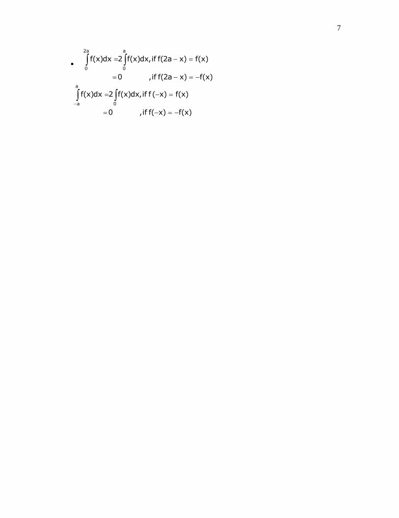
2a a

0 0

f(x)dx 2 f(x)dx,if f(2a x) f(x)

0 ,if f(2a x) f(x)

a

a 0

f(x)dx 2 f(x)dx,if f ( x) f(x)

0 ,if f( x) f(x)

1

Class XII: Mathematics

Chapter 8: Applications of Integrals

Chapter Notes

Key Concepts

1. Definite integralb

a

f(x)dx of the function f(x) from limits a to b represents

the area enclosed by the graph of the function f(x) the x axis, and the

vertical lines x= ‘a’ and x = ‘b’

2. Area function is given by

A(x) =x

a

f(x)dx , where x is a point in [a, b]

3. Area bounded by a curve, x-axis and two ordinates

Case 1: when curve lies above axis as shown below

2

.

b

aArea f(x)dx

Case 2: Curves which are entirely below the x-axis as shown below

b

aArea f(x)dx

Case 3: Part of the curve is below the x-axis and part of the curve is above

the x-axis.

c b

a cArea f(x)dx f(x)dx

4, area bounded by the curve y=f(x), the x-axis and the ordinates x=a and

x=b using elementary strip method is computed as follows

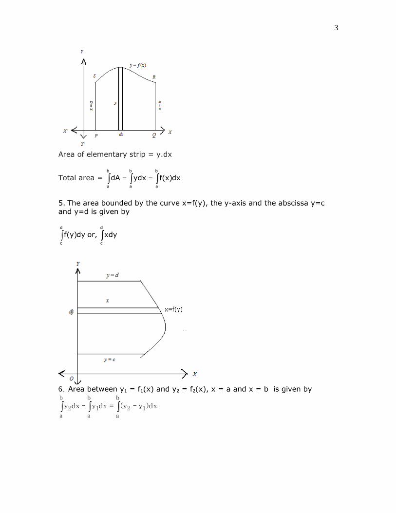
3

Area of elementary strip = y.dx

Total area = b b b

a a a

dA ydx f(x)dx

5. The area bounded by the curve x=f(y), the y-axis and the abscissa y=cand y=d is given by

d d

c c

f(y)dy or, xdy

6. Area between y1 = f1(x) and y2 = f2(x), x = a and x = b is given by

b b b

2 1 2 1

a a a

y dx - y dx = (y - y )dx

4

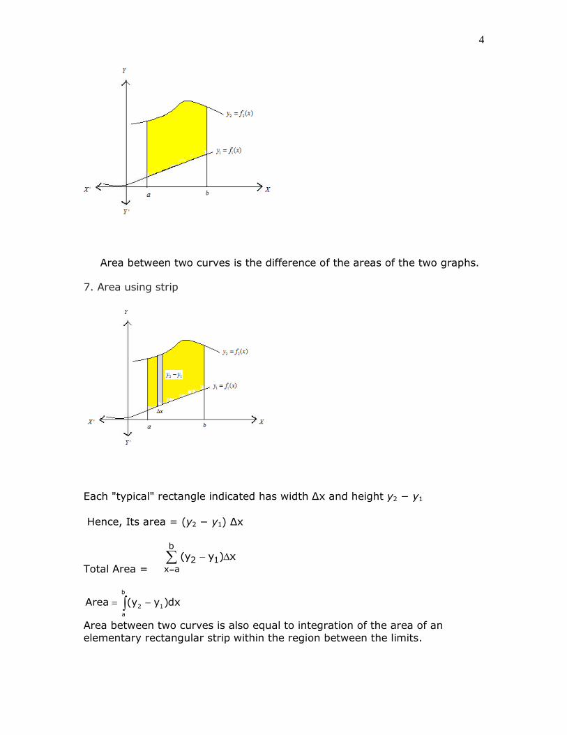
Area between two curves is the difference of the areas of the two graphs.

7. Area using strip

Each "typical" rectangle indicated has width Δx and height y2 − y1

Hence, Its area = (y2 − y1) Δx

Total Area =

b

2 1x a

(y y ) x

b

2 1

a

Area (y y )dx

Area between two curves is also equal to integration of the area of an

elementary rectangular strip within the region between the limits.

5

8. The area of the region bounded by the curve y = f (x), x-axis and the

lines x = a and x = b (b > a) is Area=b b

a a

ydx f(x)dx

9. The area of the region enclosed between two curves y = f (x), y = g

(x) and the lines x = a, x = b is

b

a

Area [f(x) g(x)]dx where, f(x) > g(x)

in [a,b]

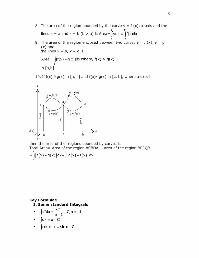
10. If f(x) ≥g(x) in [a, c] and f(x)≤g(x) in [c, b], where a< c< b

then the area of the regions bounded by curves is Total Area= Area of the region ACBDA + Area of the region BPRQB

= c b

a c

f x g x dx g x f x dx

Key Formulae

1. Some standard Integrals

n 1n x

x dx C,n 1n 1

dx x C cosxdx sinx C

6

sinxdx cosx C

2sec xdx tanx C

2cosec xdx cot x C secx tanxdx secx C cosecxcot xdx cosecx C

1

2

dxsin x C

1 x

1

2

dxcos x C

1 x

1

2

dxtan x C

1 x

1

2

dxcot x C

1 x

1

2

dxsec x C

x x 1

1

2

dxcosec x C

x x 1

x xe dx e C

xx a

a dx Cloga

1

dx log x Cx

tanxdx log secx C cot xdx log sinx C secxdx log secx tanx C cosecxdx log cosecx cot x C

2.Integral of some special functions

2 2

dx 1 x alog C

2a x ax a

2 2

dx 1 a xlog C

2a a xa x

1

2 2

dx 1 xtan C

a ax a

2 2

2 2

dxlog x x a C

x a

7

1

2 2

dx xsin C

aa x

2 2

2 2

dxlog x x a C

x a

1

Class XII: Mathematics

Chapter 9: Differential Equations

Chapter Notes

Key Concepts

1. An equation involving derivatives of dependent variable with respect toindependent variable is called a differential equation.

For example:dy

cosxdx

2 2dy x y

dx 2x

2. Order of a differential equation is the order of the highest order

derivative occurring in the differential equation.

For example: order of 3

3

d y dy3x( ) 8y 0

dxdx is 3.

3. Degree of a differential equation is the highest power (exponent) of

the highest order derivative in it when it is written as a polynomial in

differential coefficients.

Degree of equation

3 42

2

d y dy(c b) y

dxdx

is 3

4. Both order as well as the degree of differential equation are positive

intgers.

5. A function which satisfies the given differential equation is called its

solution.

6. The solution which contains as many arbitrary constants as the order

of the differential equation is called a general solution.

7. The solution which is free from arbitrary constants is called particular

solution.

8. Order of differential equation is equal to the number of arbitraryconstants present in the general solution.

9. An nth order differential equation represents an n-parameter family of

curves. 10.There are 3 Methods of Solving First Order, First Degree Differential

Equations namely

(i) Separating the variables if the variables can be separated. (ii) Substitution if the equation is homogeneous.

(iii) Using integrating factor if the equation is linear different

11.Variable separable method is used to solve equations in whichvariables can be separated i.e terms containing y should remain with

dy & terms containing x should remain with dx.

2

12.A differential equation which can be expressed in the formdy

dx= f (x,y)

or dx

dy= g(x,y) where, f (x, y) & g(x, y) are homogenous functions is

called a homogeneous differential equation.

13.Degree of each term is same in a homogeneous differential equation

14.A differential equation of the formdy

Py Qdx

, where P and Q are

constants or functions of x only is called a first order linear differential

equation. If equation is of the form dx

Px Qdy

then P and Q are

constants or functions of y

15.Steps to solve a homogeneous differential equation

dy yF(x,y) g

dx x

………(1)

Substitute y=v.x …….(2)

Differentiate (2) wrt to xdy dv

v xdx dx

……(3)

Substitute & separate the variables

dv dx

g(v) v x

Integrate,dv dx

Cg(v) v x

16. dy

Py Qdx

where, P and Q are constants

or functions of x only

Integrating factor (I.F)= e ∫Pdx

Solution: y (I.F) = ∫ (Q × I.F)dx + C

17. 1 1

dxP y Q

dy where,P1 & Q1 are constants or functions of y only

Integrating factor (I.F)= e ∫P1dy Solution: x (I.F) = ∫ (Q × I.F)dy + C

1

Class XII: Mathematics

Chapter 9: Vector Algebra

Chapter Notes

Key Concepts

1. A quantity that has magnitude as well as direction is called a vector.

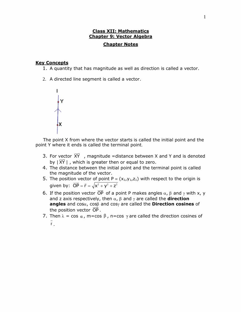
2. A directed line segment is called a vector.

The point X from where the vector starts is called the initial point and the point Y where it ends is called the terminal point.

3. For vector XY

, magnitude =distance between X and Y and is denoted

by |XY

| , which is greater then or equal to zero.

4. The distance between the initial point and the terminal point is called

the magnitude of the vector.

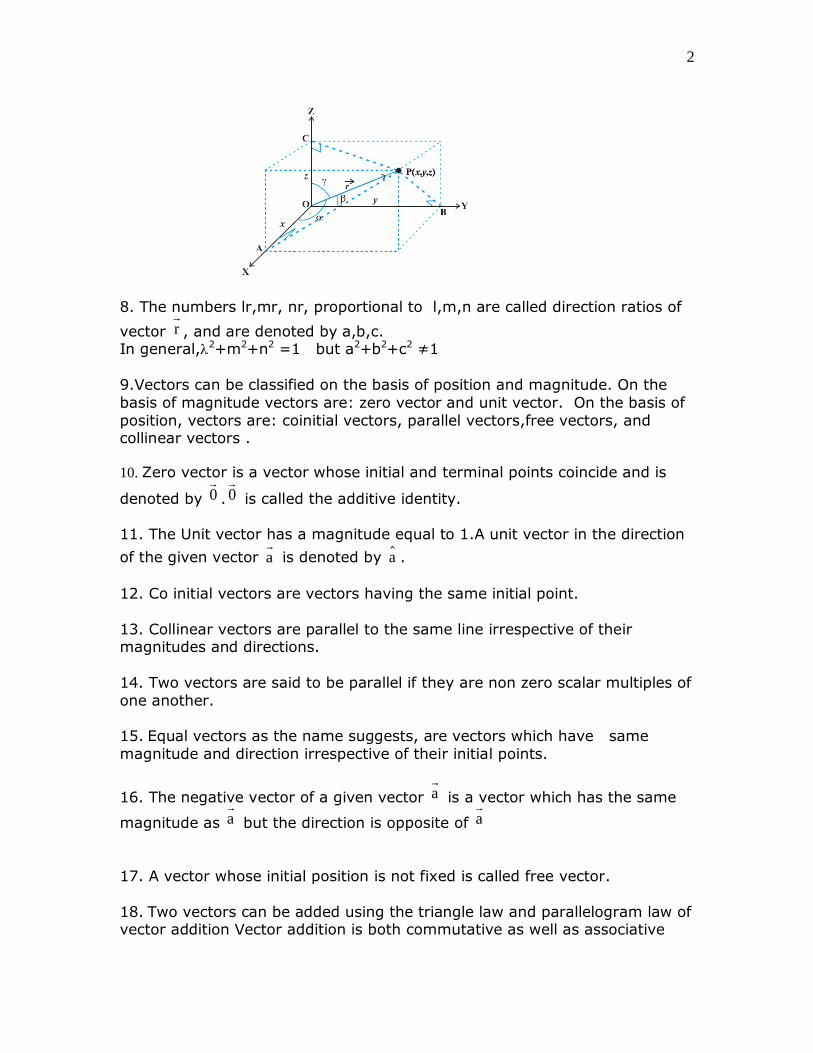
5. The position vector of point P (x1,y1,z1) with respect to the origin is

given by: 2 2 2 OP r x y z

6. If the position vector OP of a point P makes angles , and with x, y

and z axis respectively, then , and are called the direction

angles and cos, cos and cos are called the Direction cosines of

the position vector OP .

7. Then = cos α , m=cos β , n=cos γ are called the direction cosines of

r.

2

8. The numbers lr,mr, nr, proportional to l,m,n are called direction ratios of

vector r, and are denoted by a,b,c.

In general,2+m2+n2 =1 but a2+b2+c2 ≠1

9.Vectors can be classified on the basis of position and magnitude. On the

basis of magnitude vectors are: zero vector and unit vector. On the basis of

position, vectors are: coinitial vectors, parallel vectors,free vectors, and collinear vectors .

10. Zero vector is a vector whose initial and terminal points coincide and is

denoted by 0

.0

is called the additive identity.

11. The Unit vector has a magnitude equal to 1.A unit vector in the direction

of the given vector a

is denoted by a .

12. Co initial vectors are vectors having the same initial point.

13. Collinear vectors are parallel to the same line irrespective of theirmagnitudes and directions.

14. Two vectors are said to be parallel if they are non zero scalar multiples of

one another.

15. Equal vectors as the name suggests, are vectors which have same

magnitude and direction irrespective of their initial points.

16. The negative vector of a given vector a

is a vector which has the same

magnitude as a

but the direction is opposite of a

17. A vector whose initial position is not fixed is called free vector.

18. Two vectors can be added using the triangle law and parallelogram law ofvector addition Vector addition is both commutative as well as associative

3

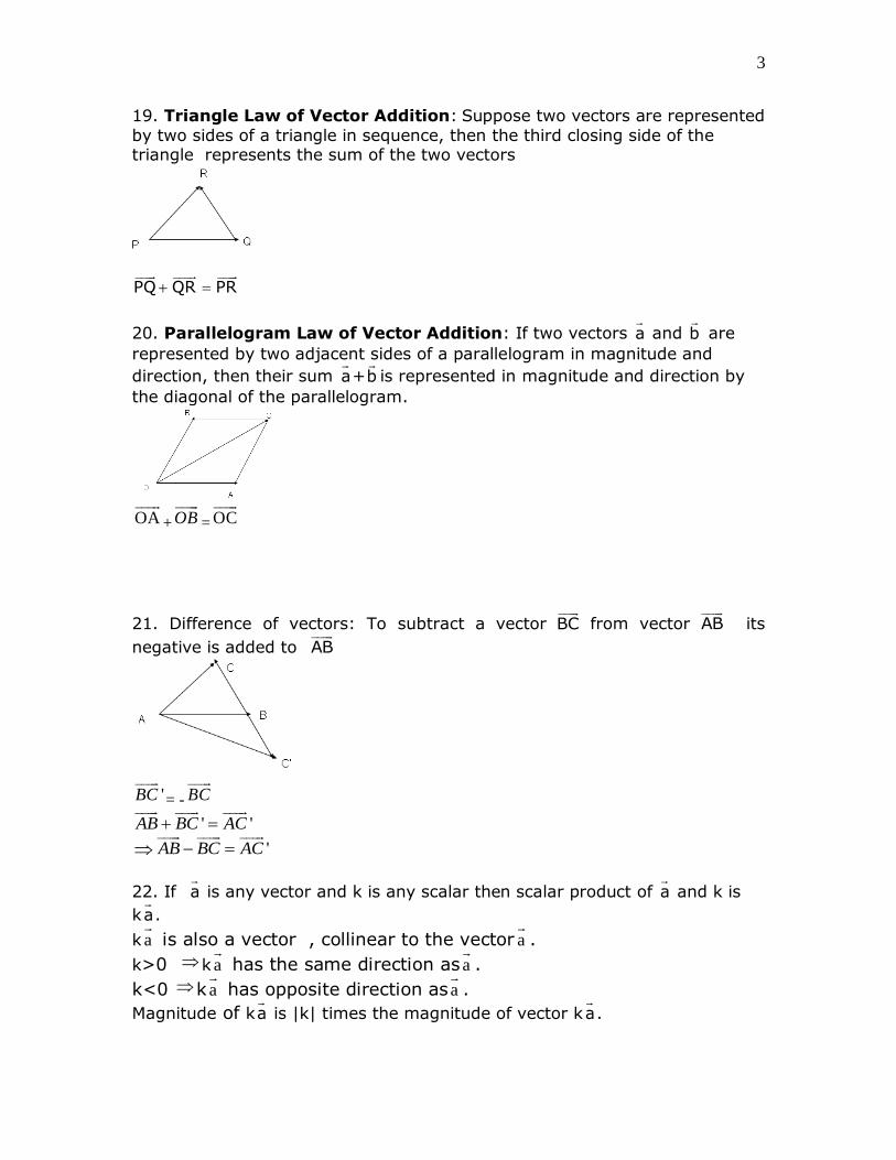
19. Triangle Law of Vector Addition: Suppose two vectors are represented

by two sides of a triangle in sequence, then the third closing side of the triangle represents the sum of the two vectors

PQ QR PR

20. Parallelogram Law of Vector Addition: If two vectors a and b

are

represented by two adjacent sides of a parallelogram in magnitude and

direction, then their sum a+b

is represented in magnitude and direction by

the diagonal of the parallelogram.

OA

+

OB = OC

21. Difference of vectors: To subtract a vector BC

from vector AB

its

negative is added to AB

'BC = -

BC

' ' AB BC AC

' AB BC AC

22. If a is any vector and k is any scalar then scalar product of a

and k is

ka.

k a is also a vector , collinear to the vector a

.

k>0 k a has the same direction asa

.

k<0 ka has opposite direction asa

.

Magnitude of ka is |k| times the magnitude of vector ka

.

4

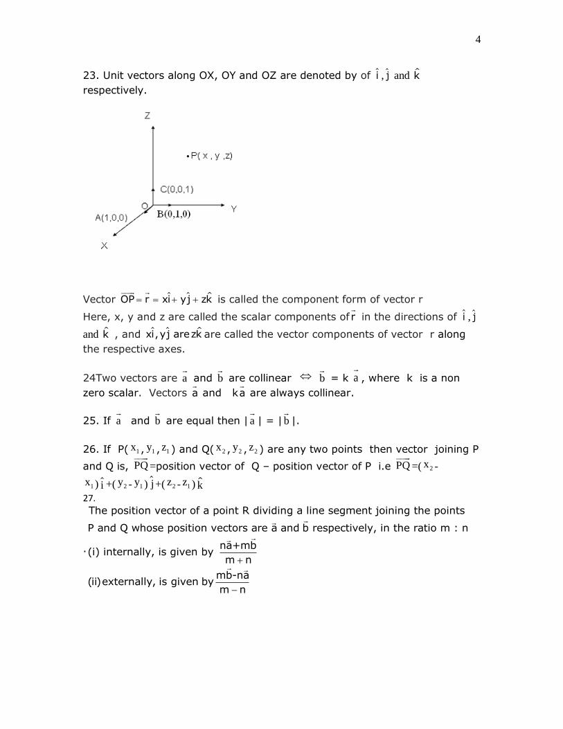
23. Unit vectors along OX, OY and OZ are denoted by of i , j and k

respectively.

Vector OP r xi yj zk

is called the component form of vector r

Here, x, y and z are called the scalar components of r

in the directions of i , j

and k , and xi,yj arezk are called the vector components of vector r along

the respective axes.

24Two vectors are a

and b

are collinear b

= k a

, where k is a non

zero scalar. Vectors a and ka

are always collinear.

25. If a

and b

are equal then | a

| = |b

|.

26. If P( 1x , 1y , 1z ) and Q( 2x , 2y , 2z ) are any two points then vector joining P

and Q is, PQ

=position vector of Q – position vector of P i.e PQ

=( 2x -

1x ) i +( 2y - 1y ) j +( 2z - 1z ) k27.

.

The position vector of a point R dividing a line segment joining the points

P and Q whose position vectors are a and b respectively, in the ratio m : n

na+mb(i) internally, is given by

m n

(ii)external

mb-naly, is given by

m n

5

28. Scalar or dot product of two non zero vectors a and b is denoted by a·b

given by a.b= |a||b|cos ,

where is the angle between vectors a and band

0

29.Projection of vector AB, making an angle of with the line L, on line L is

vector P= AB

cos

30. The vector product of two non zero vectors a

and b

denoted by a b

is

defined as ˆa b=|a||b|sin n

where θ is the angle between a

and

b,0 θ π and n̂ is a unit vector perpendicular to both a

and b

,

Here ˆa,b and n form a right handed system.

31. Area of a parallelogram is equal to modulus of the cross product of the

vectors representing its adjacent sides. 32. Vector sum of the sides of a triangle taken in order is zero.

Key Formulae

6

1. Properties of addition of vectors

1) vector addition is commutative

a b b a

2) vector addition is associative.

a (b c) (a b) c

3) 0 is additive identity for vector addition

0 0a a a

2. Magnitude or Length of vector r xi yj zk

is 2 2 2r x +y +z

3. Vector addition in Component Form: Given 1 1 11r x i y j z k

and 2 2 22r x i y j z k

then

1 2 1 2 1 21 2r r (x x )i (y y )j (z z )k

4. Difference of vectors: Given 1 1 11r x i y j z k

and 2 2 22r x i y j z k

then

1 2 1 2 1 21 2r r (x x )i (y y )j (z z )k

5. Equal Vectors: Given 1 1 11r x i y j z k

and

2 2 22r x i y j z k

then

1 2r r

if and only if 1 2 1 2 1 2x x ;y y ; z z

6. Multiplication of r xi yj zk

with scalar k is given by

kr (kx)i (ky)j (kz)k

7. For any vector r

in component form r xi yj zk

then x, y, z are the

direction ratios of r and

2 2 2

x

x y z ,

2 2 2

y

x y z ,

2 2 2

z

x y z are its

direction cosines.

8. Let a and b

be any two vectors and k and m being two scalars then

(i)ka +ma

=(k+m) a

(ii)k(ma)= (km) a

(iii)k(a+b

)=ka

+kb

9. Vectors 1 1 11r x i y j z k

and

2 2 22r x i y j z k

are collinear if

1 1 1 2 2 2x i y j z k k x i y j z k

i.e x1=kx2 ; y1 =ky2

; z1 =k z2

7

or 1 1 1

2 2 2

x y zk

x y z

10. Scalar product of vectors a and b is a.b= |a||b|cos ,

where is the angle

between vectors

11.Properties of Scalar product

(i)a·b is a real number.

(ii)If a and b

are non zero vectors then a·b

=0 a b

.

(iii) Scalar product is commutative :a·b=b.a

(iv)If =0 then a·b= a .b

(v) If = then a·b=- a . b

(vi) scalar product distributeover addition

Let a, b and cbethree vectors, then

a·(b+c)= a·b + a·c

(vii)Let a and b be two vectors, and be any scalar.

Then ( a).b=( a).b= (a.b)=a.( b)

12. Angle between two non zero vectors a and b

is given by cos =

a.b

a . b

or = cos-1 a.b

a . b

.

13. For unit vectors i , j and k

i . i = j . j = k . k =1 and i . j = j . k = k . i = 0

14. Unit vector in the direction of vector r xi yj zk

is

2 2 2

r xi yj zk

r x y z

15

1

Projection of a vector a on other vector b is given by:

bˆa.b = a. a.bb b

16. Cauchy-Schwartz Inequality:

a.b a . b

8

17.Triangle Inequality: a b a b

18. Vector r product of vectors a and b is ˆa b=|a||b|sin n

.

19. Properties of Vector Product:

(i) a b

is a vector

(ii) If a

and b are non zero vectors then a b

=0 iff a

and b

are collinear i.e

a b=0 a||b

Either =0 or =

(iii)If ,then2

a b

= a . b

(iv) vector product distribute over addition

If a,b andc are three vectors and is a scalar, then

(i) a (b+c)= a b + a c

(ii) (a b)=( a) b=a ( b)

1 2 3

1

1 2 3 1 2 3

2 3

(v) If we have two vectors a and b given in

component form as

ˆ ˆˆ ˆ ˆ ˆa=a i+a j+a k and b=b i+b j+b k

ˆˆ ˆi j k

then a b= a a a

b b b

(vi) For unit vectors i , j and k

i i = j . j = k . k =0 and i j = k , j . k = i , k . i = j

(vii) a a

= 0

as =0 sin =0

a (- a

)= 0

as = sin =0

a

b =

π

2 sin=1 a b

= a

b

n

(vii) . Angle between two non zero vectors a and b

is given by

sin = a b

a b

or = sin-1a b

a b

1

Class XII: Mathematics

Chapter 10: Three Dimensional Geometry

Chapter Notes

Key Concepts

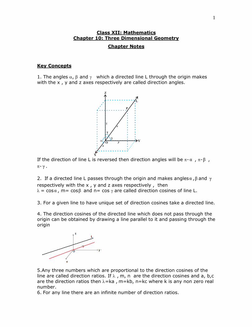
1. The angles , and which a directed line L through the origin makes

with the x , y and z axes respectively are called direction angles.

If the direction of line L is reversed then direction angles will be -α , -β ,

- γ .

2. If a directed line L passes through the origin and makes anglesα ,β and γ

respectively with the x , y and z axes respectively , then = cosα , m= cosβ and n= cos are called direction cosines of line L.

3. For a given line to have unique set of direction cosines take a directed line.

4. The direction cosines of the directed line which does not pass through theorigin can be obtained by drawing a line parallel to it and passing through the

origin

5.Any three numbers which are proportional to the direction cosines of the

line are called direction ratios. If ,m, n are the direction cosines and a, b,c

are the direction ratios then =ka ,m=kb, n=kc where k is any non zero real

number.

6. For any line there are an infinite number of direction ratios.

2

7. Direction ratios of the line joining P(x1, y1, z1) and Q(x2, y2, z2) may betaken as ,

2 1x -x, 2 1y -y

, 2 1z -zor

1 2x -x,

1 2y -y, z1-z2

8. Direction cosines of x-axis are cos0, cos 90, cos90 i.e. 1,0,0

Similarly the direction cosines of y axis are 0,1, 0 and z axis are 0,0,1

respectively.

9. A line is uniquely determined if

1) It passes through a given point and has given direction

OR 2) It passes through two given points.

10. Two lines with direction ratios a1, a2, a3 and b1, b2, b3 respectively areperpendicular if:

1 2 2 1 201a b a b c c

11. Two lines with direction ratios a1, a2, a3 and b1, b2, b3 respectively are

parallel if 1

2

a

a= 1

2

b

b= 1

2

c

c

12. The lines which are neither intersecting nor parallel are called as skew

lines. Skew lines are non coplanar i.e. they don’t belong to the same 2D plane.

GE and DB are skew lines.

13. Angle between skew lines is the angle between two intersecting lines

drawn from any point (preferably through the origin) parallel to each of the skew lines.

14. If two lines in space are intersecting then the shortest distance between

them is zero.

3

15. If two lines in space are parallel, then the shortest distance between

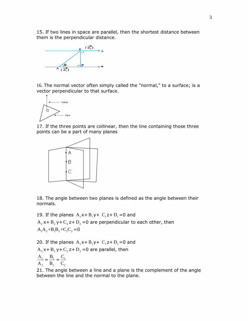
them is the perpendicular distance.

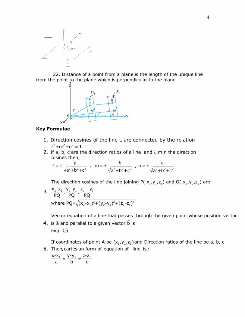
16. The normal vector often simply called the "normal," to a surface; is a

vector perpendicular to that surface.

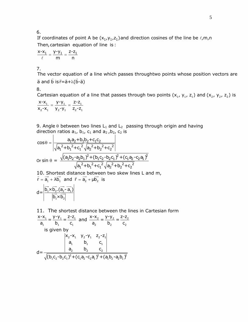
17. If the three points are collinear, then the line containing those threepoints can be a part of many planes

18. The angle between two planes is defined as the angle between their

normals.

19. If the planes 1A x+ 1B y+ 1C z+ 1D =0 and

2A x+ 2B y+ 2C z+ 2D =0 are perpendicular to each other, then

1 2 1 2 1 2A A +B B +C C =0

20. If the planes 1A x+ 1B y+ 1C z+ 1D =0 and

2A x+ 2B y+ 2C z+ 2D =0 are parallel, then

1

2

A

A= 1

2

B

B= 1

2

C

C

21. The angle between a line and a plane is the complement of the anglebetween the line and the normal to the plane.

4

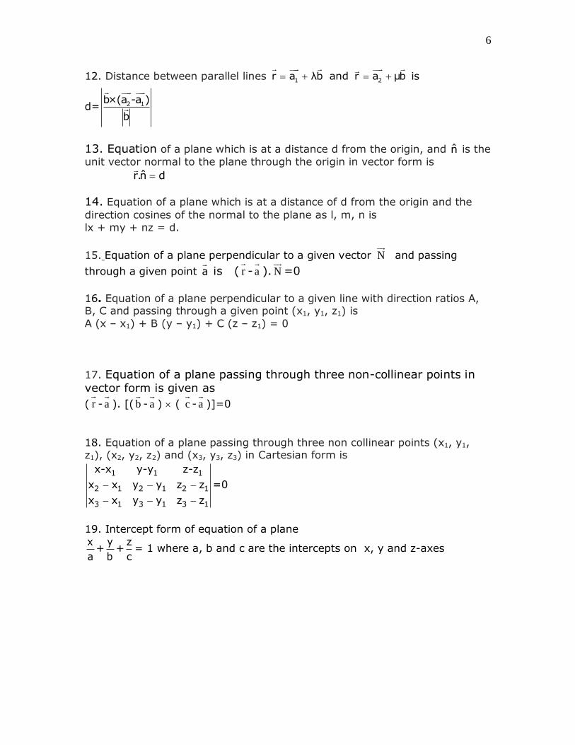
22. Distance of a point from a plane is the length of the unique line

from the point to the plane which is perpendicular to the plane.

Key Formulae

1. Direction cosines of the line L are connected by the relation2 2 2+m +n 1

2. If a, b, c are the direction ratios of a line and ,m,n the direction

cosines then,

2 2 2

a

a +b +c ,

2 2 2

bm

a +b +c ,

2 2 2

cn

a +b +c

3.

1 1 1 2 2 2

2 1 2 1 2 1

2 2 2

2 1 2 1 2 1

The direction cosines of the line joining P( x ,y ,z ) and Q( x ,y ,z ) are

x -x y -y z z, ,

PQ PQ PQ

where PQ= (x -x ) +(y -y ) +(z -z )

4.

Vector equation of a line that passes through the given point whose position vector

is a and parallel to a given vector b is

r=a+ b

5. 1 1 1

1 1 1

If coordinates of point A be (x ,y ,z )and Direction ratios of the line be a, b, c

Then,cartesian form of equation of line is :

x-x y-y z-z

a b c

5

6.

1 1 1

1 1 1

If coordinates of point A be (x ,y ,z )and direction cosines of the line be ,m,n

Then,cartesian equation of line is :

x-x y-y z-z

m n

7.

The vector equation of a line which passes throughtwo points whose position vectors are

a and b isr=a+ (b-a)

8.

1 1 1 2 2 2

1 1 1

2 1 2 1 2 1

Cartesian equation of a line that passes through two points (x , y , z ) and (x , y , z ) is

x-x y-y z-z

x -x y -y z -z

9. Angle between two lines L1 and L2 passing through origin and having

direction ratios a1, b1, c1 and a2 ,b2, c2 is

1 2 1 2 1 2

2 2 2 2 2 21 1 1 2 2 2

a a +b b +c ccos

a +b +c a +b +c

Or sin = 2 2 2

1 2 2 1 1 2 2 1 1 2 2 1

2 2 2 2 2 21 1 1 2 2 2

(a b -a b ) +(b c -b c ) +(c a -c a )

a +b +c a +b +c

10. Shortest distance between two skew lines L and m,

1 1 2 2r a λb and r a μb

is

d= 1 2 2 1

1 2

b ×b .(a - a )

b ×b

11. The shortest distance between the lines in Cartesian form

1

1

x-x

a= 1

1

y-y

b= 1

1

z-z

c and 2

2

x-x

a= 2

2

y-y

b= 2

2

z-z

c

is given by

d=

2 1 2 1 2 1

1 1 1

2 2 2

2 2 2

1 2 2 1 1 2 2 1 1 2 2 1

x -x y -y z -z

a b c

a b c

(b c -b c ) +(c a -c a ) +(a b -a b )

6

12. Distance between parallel lines 1 2r a λb and r a μb

is

d= 2 1b×(a -a )

b

13. Equation of a plane which is at a distance d from the origin, and n̂ is the

unit vector normal to the plane through the origin in vector form is

ˆr.n d

14. Equation of a plane which is at a distance of d from the origin and the

direction cosines of the normal to the plane as l, m, n is

lx + my + nz = d.

15. Equation of a plane perpendicular to a given vector N

and passing

through a given point a is ( r

- a). N

=0

16. Equation of a plane perpendicular to a given line with direction ratios A,B, C and passing through a given point (x1, y1, z1) is

A (x – x1) + B (y – y1) + C (z – z1) = 0

17. Equation of a plane passing through three non-collinear points invector form is given as

( r- a

). [(b

- a

) ( c- a

)]=0

18. Equation of a plane passing through three non collinear points (x1, y1,z1), (x2, y2, z2) and (x3, y3, z3) in Cartesian form is

1 1 1

2 1 2 1 2 1

3 1 3 1 3 1

x-x y-y z-z

x x y y z z

x x y y z z

=0

19. Intercept form of equation of a plane

x

a+

y

b+

z

c= 1 where a, b and c are the intercepts on x, y and z-axes

7

respectively.

20. Any plane passing thru the intersection of two planes r. 1n

=d1 and

r. 2n

=d2 is given by,

1 2 1 2r. n λn d λd

21. Cartesian Equation of plane passing through intersection of two planes

(A1x +B1y +C1z-d1 + (A2x+B2y+C2z-d2) = 0

22. The given lines 1 1 2 2r a λb and r a μb

are coplanar if and only

02 1 1 2a a . b b

23. Let 1 1 1(x ,y ,z ) and 2 2 2(x ,y ,z ) be the coordinates of the points M and N

respectively.

Let a1, b1, c1 and a2, b2, c2 be the direction ratios of 1b

and 2b

respectively.

The given lines are coplanar if and only if

2 1 2 1 2 1

1 1 1

2 2 2

x -x y -y z -z

a b c

a b c

=0

24. If 1n

and 2n

are normals to the planes

1r.n

=d1and 2r.n

= d2 and is the angle between the normals drawn from

some common point then

cos = 1 2

1 2

n .n

n n

25. Let θ is the angle between two planes A1x+B1y+C1z+D1=0,

A2x+B2y+C2z+D2=0

The direction ratios of the normal to the planes are A1, B1, C1 and A2, B2,, C2.

cos = 1 2 1 2 1 2

2 2 2 2 2 2

1 1 1 2 2 2

A A +B B +C C

A +B +C A +B +C

8

26. The angle between the line and the normal to the plane is given by

cos=b.n

b n

or sin =b.n

b n

where

27. Distance of point P with position vector a from a plane r.N

=d is

a.N-d

N

where N

is the normal to the plane

28. The length of perpendicular from origin O to the plane r.N

=d is d

N

where N

is the normal to the plane.

1

Class XII: Math

Chapter 12: Linear Programming

Chapter Notes

Key Concepts

1. Linear programming is the process of taking various linear inequalitiesrelating to some situation, and finding the "best" value obtainable under

those conditions. 2. Linear programming is part of a very important area of mathematics

called "optimisation techniques.

3. Type of problems which seek to maximise (or minimise) profit (or cost)form a general class of problems called optimisation problems.

4. A problem which seeks to maximise or minimise a linear function subject

to certain constraints as determined by a set of linear inequalities is called an optimisation problem.

5. A linear programming problem may be defined as the problem ofmaximising or minimising a linear function subject to linear constraints.

The constraints may be equalities or inequalities.

6. Objective Function: Linear function Z = ax + by, where a, b are

constants, x and y are decision variables, which has to be maximised or

minimised is called a linear objective function. Objective function

represents cost, profit, or some other quantity to be maximised of minimised subject to the constraints.

7. The linear inequalities or equations that are derived from the applicationproblem are problem constraints.

8. The linear inequalities or equations or restrictions on the variables of a

linear programming problem are called constraints.

9. The conditions x ≥ 0, y ≥ 0 are called non – negative restrictions. Non -

negative constraints included because x and y are usually the number of items produced and one cannot produce a negative number of items. The

smallest number of items one could produce is zero. These are not

(usually) stated, they are implied.

10.A linear programming problem is one that is concerned with finding the

optimal value (maximum or minimum value) of a linear function (called

objective function) of several variables (say x and y), subject to the conditions that the variables are non – negative and satisfy a set of

linear inequalities (called linear constraints).

2

11.In Linear Programming the term linear implies that all the

mathematical relations used in the problem are linear and Programming refers to the method of determining a particular

programme or plan of action.

12. Forming a set of linear inequalities (constrains) for a given situation iscalled formulation of the linear programming problem or LPP.

13. Mathematical Formulation of Linear Programming Problems

Step I: In every LPP certain decisions are to be made. These decisions are represented by decision variables. These decision

variables are those quantities whose values are to be determined.

Identify the variables and denote them by x1, x2, x3, …. Or x,y and z etc

Step II: Identify the objective function and express it as a linear

function of the variables introduced in step I.

Step III: In a LPP, the objective function may be in the form of maximising profits or minimising costs. So identify the type of

optimisation i.e., maximisation or minimisation.

Step IV: Identify the set of constraints, stated in terms of decision variables and express them as linear inequations or equations as the

case may be.

Step V: Add the non-negativity restrictions on the decision variables, as in the physical problems, negative values of decision variables have

no valid interpretation.

14. General LPP is of the form Max (or min) Z = c1x1 + c2x2 + … +cnxn

c1,c2,….cn are constants

x1, x2, ....xn are called decision variable. s.t Ax ()B and xi 0

3

15. A linear inequality in two variables represents a half plane geometrically.

Types of half planes

16.The common region determined by all the constraints including non –

negative constraints x, y ≥ 0 of a linear programming problem is called

the feasible region (or solution region) for the problem. The region

other than feasible region is called an infeasible region.

17. Points within and on the boundary of the feasible region represent

feasible solution of the constraints.

18. Any point in the feasible region that gives the optimal value (maximum

or minimum) of the objective function is called an optimal solution.

19. Any point outside the feasible region is called an infeasible solution.

4

20.A corner point of a feasible region is the intersection of two boundary

lines.

21.A feasible region of a system of linear inequalities is said to be bounded if

it can be enclosed within a circle.

22.Corner Point Theorem 1: Let R be the feasible region (convex polygon)

for a linear programming problem and let Z = ax + by be the objective

function. When Z has an optimal value (maximum or minimum), where

the variables x and y are subject to constraints described by linear

inequalities, this optimal value must occur at a corner point (vertex) of

the feasible region.

23. Corner Point Theorem 2: Let R be the feasible region for a linear

programming problem, and let Z = ax + by be the objective function. If

R is bounded, then the objectives function Z has both a maximum and a

minimum value on R and each of these occurs at a corner point (vertex)

of R.

24. If R is unbounded, then a maximum or a minimum value of the

objectives functions may not exist.

25.The graphical method for solving linear programming problems in two

unknowns is as follows.

A. Graph the feasible region.

B. Compute the coordinates of the corner points.

C. Substitute the coordinates of the corner points into the objective

function to see which gives the optimal value.

D. When the feasible region is bounded, M and m are the maximum and

minimum values of Z.

E. If the feasible region is not bounded, this method can be misleading:

optimal solutions always exist when the feasible region is bounded, but

may or may not exist when the feasible region is unbounded.

(i) M is the maximum value of Z, if the open half plane determined by ax

+ by > M has no point in common with the feasible region. Otherwise, Z

has no maximum value.

(ii) Similarly, m is the minimum value of Z,if the open half plane

5

determined by ax+by<m has no point in common with the feasible

region. Otherwise, Z has no minimum value.

26.Points within and on the boundary of the feasible region represent

feasible solutions of the constraints.

27. If two corner points of the feasible region are both optimal solutions of

the same type, i.e., both produce the same maximum or minimum, then

any point on the line segment joining these two points is also an optimal

solution of the same type.

28. Types of Linear Programming Problems

1 Manufacturing problems : Problems dealing in finding the number

of units of different products to be produced and sold by a firm when

each product requires a fixed manpower, machine hours, labour hour

per unit of product in order to make maximum profit.

2 Diet problem: Problems, dealing in finding the amount of different

kinds of nutrients which should be included in a diet so as to minimise

the cost of the desired diet such that it contains a certain minimum

amount of each constituent/nutrients.

3 Transportation problems: Problems dealing in finding the

transportation schedule of the cheapest way to transpor a product

from plants/factories situated at different locations to different

markets.

29. Advantages of LPP

(i) Linear programming technique helps to make the best possible use of

available productive resources (such as time, labour, machines etc.)

(ii) A significant advantage of linear programming is highlighting of such

bottle necks.

30. Disadvantages of LPP

(i) Linear programming is applicable only to problems where the constraints

and objective functions are linear i.e., where they can be expressed as

6

equations which represent straight lines.

(ii) Factors such as uncertainty, weather conditions etc. are not taken into

consideration.

1

Class XII: Mathematics

Chapter : Probability

Chapter Notes

Key Concepts

1. The probability that event B will occur if given the knowledge that event Ahas already occurred is called conditional probability. It is denoted as

P(B|A).

2. Conditional probability of B given A has occurred P(B|A) is given by the

ratio of number of events favourable to both A and B to number of events

favourable to A.

3. E and F be events of a sample space S of an experiment, then

(i). P(S|F) = P(F|F)=1

(ii) For any two events A and B of sample space S if F is another event such that P(F) 0

P ((A B) |F) = P (A|F)+P (B|F)–P ((A B)|F)

(iii) P(E’|F) = 1-P(E|F)

4. Two events A and B are independent if and only if the occurrence of A

does not depend on the occurrence of B and vice versa.

5. If events A and B are independent then P(B|A) = P(A) and P(A|B)=P(A)

6. Three events A,B, C are independent if they are pair wise independent i.e P(A B) = P(A) .P(B) , P (A C) = P (A). P (C), P(B C) = P(B) .P(C)

7. Three events A,B, C are independent if P(A B C) = P(A). P (B). P (C)

Independence implies pair wise independence, but not conversely.

8. In the case of independent events, event A has no effect on the probability

of event B so the conditional probability of event B given event A has already occurred is simply the probability of event B, P(B|A)=P(B).

9. If E and F are independent events then so are the events (i)E’ and F

(ii)E and F’

(iii)E’ and F’

10. If A and B are events such that B then B is said to affect A

i) favourably if P(A|B) > P(A)

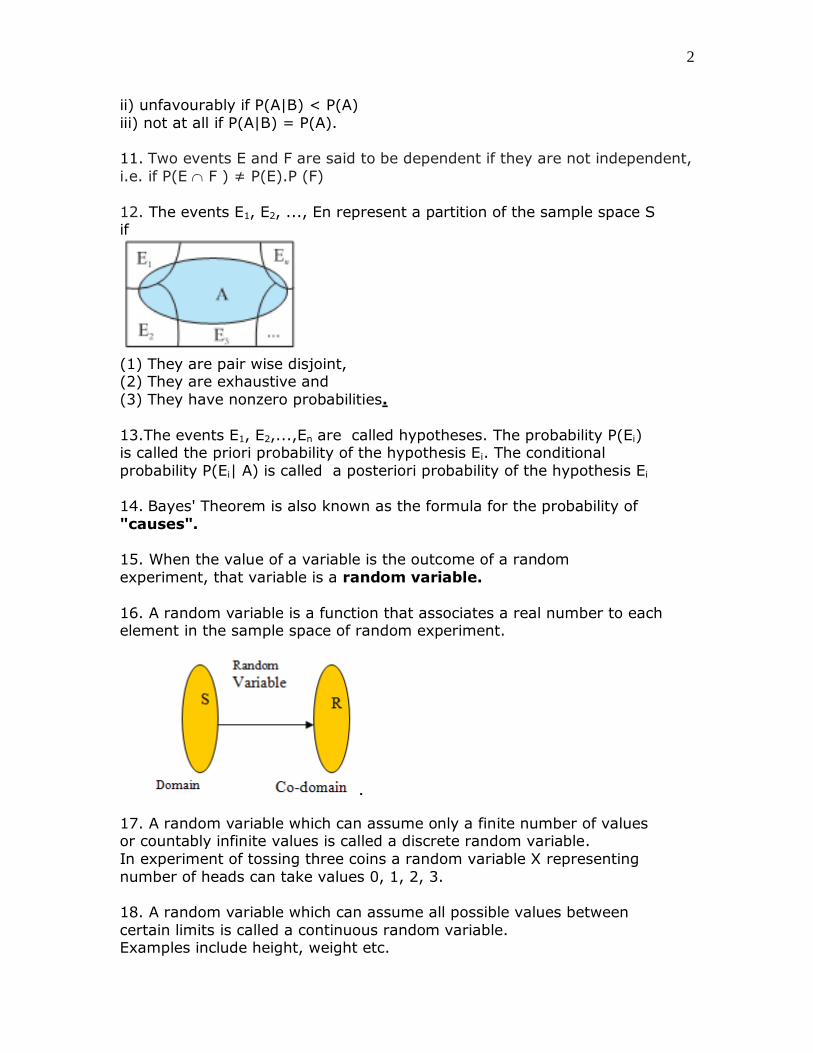
2

ii) unfavourably if P(A|B) < P(A)

iii) not at all if P(A|B) = P(A).

11. Two events E and F are said to be dependent if they are not independent,

i.e. if P(E F ) ≠ P(E).P (F)

12. The events E1, E2, ..., En represent a partition of the sample space Sif

(1) They are pair wise disjoint, (2) They are exhaustive and

(3) They have nonzero probabilities.

13.The events E1, E2,...,En are called hypotheses. The probability P(Ei)is called the priori probability of the hypothesis Ei. The conditional

probability P(Ei| A) is called a posteriori probability of the hypothesis Ei

14. Bayes' Theorem is also known as the formula for the probability of

"causes".

15. When the value of a variable is the outcome of a random

experiment, that variable is a random variable.

16. A random variable is a function that associates a real number to eachelement in the sample space of random experiment.

17. A random variable which can assume only a finite number of valuesor countably infinite values is called a discrete random variable.

In experiment of tossing three coins a random variable X representing

number of heads can take values 0, 1, 2, 3.

18. A random variable which can assume all possible values between

certain limits is called a continuous random variable. Examples include height, weight etc.

3

19. The probability distribution of a random variable X is the system ofnumbers

1

1

1

0 1 1 2 3

n

n

n

i ii

X : x x ..... x

P(X) : p p ..... p

where p , p ,i , , ,....,n

The real numbers x1, x2,..., xn are the possible values of the random variable

X and pi (i = 1,2,..., n) is the probability of the random variable X taking the

value xi i.e. P(X = xi) = pi

20. In the probability distribution of x each probability pi is non

negative, and sum of all probabilities is equal to 1.

21. Probability distribution of a random variable x can be represented

using bar charts.

X 1 2 3 4

P(X) .1 .2 .3 .4

Tabular Representation

Graphical Representation

22. The expected value of a random variable indicates its average or

central value.

23. The expected value of a random variable indicates its average or central

value. It is a useful summary value of the variable's distribution.

24. Let X be a discrete random variable which takes values x1, x2, x3,…xn

with probability pi = P{X = xi}, respectively. The mean of X, denoted by μ, is

summation pixi 25. Trials of a random experiment are called Bernoulli trials, if they satisfy

the following conditions :

(i) There should be a finite number of trials. (ii) The trials should be independent.

(iii) Each trial has exactly two outcomes: success or failure.

(iv) The probability of success remains the same in each trial.

4

26. Binomial distribution is the discrete probability distribution of the

number of successes in a sequence of n independent binomial experiments, each of which yields success with probability p.

27. Bernoulli experiment is a random experiment whose trials have two

outcomes that are mutually exclusive: they are, termed, success and failure.

28. Binomial distribution with n-Bernoulli trials, with the probability of

success in each trial as p, is denoted by B (n, p). n and p are called the parameters of the distribution.

29. The random variable X follows the binomial distribution with parametersn and p, we write XK ~ B(n, p). The probability of getting exactly k successes

in n trials is given by the probability mass function

P (X = k) = nCk q n–k pk

30. Equal means of two probability distributions does not imply same

distributions.

Key Formulae

1. 0 ≤ P (B|A) ≤ 1

2. If E and F are two events associated with the same sample space of arandom experiment, the conditional probability of the event E given

that F has occurred, i.e. P (E|F) is given by

0n(E F)

P(E|F) providedP(F)n(F)

or

0n(E F)

P(F |E) providedP(E)n(E)

3. Multiplication Theorem:

(a) For two events

Let E and F be two events associated with a sample space S. P (E F) = P (E) P (F|E) = P (F) P (E|F) provided P (E) 0 and

P (F) 0.

5

(b) For three events:

If E, F and G are three events of sample space S,

P(E F G) = P (E) P (F|E) P(G|(E F)) = P (E) P(F|E) P(G|EF)

4. Multiplication theorem for independent Events

(i) P (E F) = P(E)P(F)

(ii) P(E F G) = P(E)P(F)P(G)

5. Let E and F be two events associated with the same randomexperiment Two events E and F are said to be independent, if

(i) P(F|E) = P (F) provided P (E) 0 and

(ii) P (E|F) = P (E) provided P (F) 0

(iii)P(E F) = P(E) . P (F)

6. Occurrence of atleast one of the two events A or B

P(AB) =1-P(A’)P(B’)

7. A set of events E1, E2, ..., En is said to represent a partition of the samplespace S if

(a) Ei Ej = , i ≠j, i, j = 1, 2, 3, ..., n

(b) E1 E2 En= S

(c) P(Ei) > 0 for all i = 1, 2, ..., n.

8. Theorem of Total Probability

Let {E1, E2,...,En} be a partition of the sample space S, and suppose that each of the events E1, E2,..., En has nonzero probability of occurrence. Let A

be any event associated

with S, then P(A) = P(E1) P(A|E1) + P(E2) P(A|E2) + ... + P(En) P(A|En)

= 1

n

j jj

P E P A |E

9. Bayes’ Theorem

If E1, E2 ,..., En are n non-empty events which constitute a partition of

sample space S and A is any event of nonzero probability, then

1

i i

n

j jj

P(E )P(A |E )P(Ei | A)

P(E )P(A |E )

for any I =1,2,3,…n

10.The mean or expected value of a random variable X, denoted by E(X) or

μ is defined as

E (X) = μ = 1

n

i ii

xp

6

11. The variance of the random variable X, denoted by Var (X) or x2 is

defined as

22 2

1

n

x i ii

Var(X) x p(x ) E(X )

Var (X) = E(X2) – [E(X)]2

12. Standard Deviation of random variable X:

2

1

n

x i ii

Var(X) x p(x )

13. For Binomial distribution B (n, p),

P (X = x) = nCx q n–x px, x = 0, 1,..., n (q = 1 – p)

14. Mean and Variance of a variable X following Binomial distribution

E (X) = μ = np Var (X) = npq

Where n is number of trials, p = probability of success

q = probability of failures

15. Standard Deviation of a variable X following Binomial distribution

x Var(X) npq