xrf and appropriate quality control - clu-in.org

XRF Web Seminar Module 5 – Quality Control

August 2008 5-1

There are still issues surrounding the acceptance of XRF data for risk assessment and the collection of definitive vs. screening data. A good QC program is critical to XRF data moving beyond the screening designation to more definitive uses such as delineation confirmation and risk assessment.

The focus of today’s session is on the types of QC samples that are available, how they can be used, some examples of tools and strategies used successfully at other sites, and some potential pitfalls to look out for that highlight the critical need for good XRF QC.

5-1

XRF and Appropriate Quality Control

CLU-IN Studios Web Seminar

August 18, 2008

Stephen DymentUSEPA

Technology Innovation Field Services [email protected]

Module 5 – Quality Control XRF Web Seminar

5-2 August 2008

When you registered, you were directed to this seminar's specific URL, which is the front page of today's seminar. The Front Page of the Web cast contains a short abstract of today's session. We have also included pictures and short biosketches of the presenters. Please note the presenters' email addresses are hotlinked on that page in case you have any questions for one of them after today's presentation.

For those of you joining us via the phone lines, we request that you put your phone on mute for the seminar. We will have Q&A sessions at which point you are welcome to take your phone off mute and ask the question. If you do not have a mute button on your phone, we ask that you take a moment RIGHT NOW to hit *6 to place your phone on MUTE. When we get to the question and answer periods you can hit #6 to unmute the phone. This will greatly reduce the background noises that can disrupt the quality of the audio transmission.

Also, please do not put us on HOLD. Many organizations have hold music or advertisements that can be very disruptive to the call. Again, keep us on MUTE. DO NOT put us on HOLD.

Also, if you experience technical difficulties with the audio stream, you may use the ? icon to alert us to the technical difficulties you are encountering. Please include a telephone number where you can be reached and we will try to help you troubleshoot your problem.

5-2

How To . . .

Ask questions »“?” button on CLU-IN page

Control slides as presentation proceeds»manually advance slides

Review archived sessions»http://www.clu-in.org/live/archive.cfm

Contact instructors


August 2008 5-3

Instructor contact information:

Deana Crumbling, U.S. EPA Phone: (703) 603-0643 Fax: (703) 603-9135 E-mail: [email protected] Robert Johnson, Argonne National Laboratory Phone: (630) 252-7004 Fax: (630) 252-3611 E-mail: [email protected] Stephen Dyment, U.S. EPA Phone: (703) 603-9903 Fax: (703) 603-9135 E-mail: [email protected]


5-4 August 2008

5-3

Q&A For Session 4 – DMA


August 2008 5-5

This picture represents what some people may feel when it comes to QC - if we pretend it doesn’t exist then we shouldn’t have an issue. In the past, we took a few took a few splits, got a good R2 value, and knew the XRF was good. From there people would operate the instrument in unconcerned bliss.

However, there are a whole host of issues that can arise when using XRF at your site. To spot those issues before they have a significant impact on a project requires a QC program. This slide shows a list of the types of QC issues encountered when using FP XRF and these issues will be addressed in this module.

Matrix effects example: moisture greater than 20% can impact performance. High levels of moisture can absorb or reflect x-rays resulting in bias.

For in-situ operation good window contact and surface preparation are key.

5-4

What Can Go Wrong with an XRF?

Initial or continuing calibration problemsInstrument driftWindow contaminationInterference effectsMatrix effectsUnacceptable detection limitsMatrix heterogeneity effectsOperator errors


5-6 August 2008

As highlighted in previous modules, sample variability is the driver in terms of overall measurement uncertainty or variability. The next few slides illustrate the effects of within-sample variability. Care should be taken when generalizing in terms of which analytical methods provide better control on variability.

Within-sample variability can impact data

quality more than the analytical

method

5-5(continued)


August 2008 5-7

Samples were archives (20-30 grams in a sandwich bag) analyzed for arsenic by ICP in 2005 by a Regional laboratory and again in 2006 by ERT. Correlation coefficients were better for both the Innov-X and Niton instrument cup samples and corresponding ICP analysis.

5-6

Within-sample variability can impact data

quality more than the analytical

method


5-8 August 2008

It is difficult to generalize as to whether ICP or XRF is more precise, even within the same sample.

0 50 100 150 200 250 300 350

As conc (ppm)

XRF ave

ICP ave

2815 F1-SS1-3 jar As CI

width 86 40

LCL 250 202

XRF ave ICP ave

0 50 100 150 200 250 300 350

As conc (ppm)

XRF ave

ICP ave

2815 F1-SS1-3 jar As CI

width 86 40

LCL 250 202

XRF ave ICP ave

0 50 100 150 200

Pb conc (ppm)

XRF ave

ICP ave

2815 F1-SS1-3 jar Pb CI

width 18 84

LCL 165 95

XRF ave ICP ave

0 50 100 150 200

Pb conc (ppm)

XRF ave

ICP ave

2815 F1-SS1-3 jar Pb CI

width 18 84

LCL 165 95

XRF ave ICP ave

Sometimes Sometimes ICP is more ICP is more preciseprecise……

……sometimes sometimes XRF isXRF is

Triplicate subsamples of the same (<10 mesh) sample analyzed by both ICP & XRF

CI results for As & Pb shown here

95% Confidence Interval (CI) Bar Graphs

Arsenic CI Graph

Lead CI Graph

= 294

= 137= 174

= 203

5-7


August 2008 5-9

In this series of images, the XRF average is always greater than the ICP. In most cases the XRF number can be considered conservative. If field based action levels are being used in addition to these conservative XRF concentrations, the project team can be very confident that the decision errors will be minimalized. However, for most applications the established laboratory method (in this case ICP) is expected to better represent the true mean.

0 200 400 600 800 100012001400

Pb conc (ppm)

XRF ave

ICP ave

2815 SC5 bag Pb CI

width 644 231

LCL 685 422

XRF ave ICP ave

0 200 400 600 800 100012001400

Pb conc (ppm)

XRF ave

ICP ave

2815 SC5 bag Pb CI

width 644 231

LCL 685 422

XRF ave ICP ave

95% CI Bar Graphs for Another Sample

= 864

0 40 80 120 160 200

As conc (ppm)

XRF ave

ICP ave

2815 SC5 bag As CI

width 59 151

LCL 99 15

XRF ave ICP ave

0 40 80 120 160 200

As conc (ppm)

XRF ave

ICP ave

2815 SC5 bag As CI

width 59 151

LCL 99 15

XRF ave ICP ave = 91

= 538

= 129Here the situation is reversed for another sample from the same yard.

Sometimes Sometimes XRF is more XRF is more

preciseprecise……

……sometimes sometimes ICP isICP is

Arsenic CI Graph

Lead CI Graph

5-8


5-10 August 2008

This graphic illustrates the huge impact particle size can have on both concentration and variability of results.

95% CI Bar Graphs for Particle Size Effects

= 438 = 129

= 129 = 129

Particle Sizes

all <10 mesh = crushed soil put thru 10-mesh sieve & analyze all going thru

10-60 mesh = above then put thru 60-mesh sieve & what is retained on 60-mesh is analyzed

<60 mesh = that going thru 60-mesh sieve & is analyzed

40 140 240 340 440 540 640 740

As conc (ppm)

<60

10-60

all <10

2505 PT1-S jar Particle Size Effects for As

CI width 70 171 271

LCL 513 312 397

<60 10-60 all <10

40 90 140 190 240 290 340 390 440

Pb conc (ppm)

<60

10-60

all <10

2505 PT1-S jar Particle Size Effects for Pb

CI width 23 108 124

LCL 381 260 313

<60 10-60 all <10

Ave = 533

Ave = 397

Ave = 548

Ave = 375

Ave = 314

Ave = 392

5-9


August 2008 5-11

What can be done to stem the tide of uncertainty?

5-10

What Can We Do?

(continued)


5-12 August 2008

Recognize the advantages and limitation of XRF and laboratory methods: Both XRF and laboratory methods are not without advantages and limitations. By recognizing those, the project team can rely on the other to strengthen data sets and decisions.

Recognize that uncertainty exists: It is important to stop ignoring uncertainty. NIST recognizes it, and we should too. Fortunately, there are techniques to manage these uncertainties and strengthen environmental decisions.

Perform a demonstration of method applicability (DMA): Even simple applications can provide critical information that drives effective and efficient use of FPXRF. DMAs are important for the following reasons:

» A form of “front end” quality control

» Typically built around site-specific sampled media (archived material or can be collected explicitly for the study)

» Useful for establishing expected performance and identify ways to optimize sampling/analysis

» Useful for “flushing out” potential analytical, sample preparation, throughput, and logistical problems

» Useful for identifying QC requirements for full deployment

5-11

What Can We Do?

Recognize the advantages and limitations of XRF and laboratory methods Recognize that uncertainty existsPerform a demonstration of method applicability study (DMA)Structure your QA/QC program to adaptively manage uncertaintyUse collaborative data sets- powerful weight of evidence and take advantage of both methods


August 2008 5-13

Structure your QA/QC program to adaptively manage uncertainty: Use the DMA to identify the greatest uncertainties and manage resources to control those, but allow sufficient flexibility to adaptively manage QC issues as they arise. Illustrates the need for qualified field and support teams that provide “real-time” data interpretation, troubleshooting, and feedback.

Use collaborative data sets – powerful weight of evidence and take advantage of both methods: Collaborative data sets give the power of high density real time information from XRF and the targeted high precision and well documented laboratory data that allow those “XRF skeptics” a level of comfort. Collaborative data sets illustrate some of the challenges that arise from solely using lower density laboratory analyses.


5-14 August 2008

Certified concentrations based on two or more independent methods requiring complete sample decomposition or nondestructive analysis: The table on the right-hand side of this slide shows the National Institute of Standards and Technology SRMs. The certified values are weighted means of results from two or more independent analytical methods, or the mean of results from a single definitive method, except for mercury. Mercury certification is based on cold vapor atomic absorption spectrometry used by two different laboratories employing different methods of sample preparation prior to measurement. The weights for the weighted means were computed according to the iterative procedure of Paule and Mandel [1]. Note that there are uncertainties associated with the reference values.

Some of the most homogenous and well characterized material out there: The stated uncertainties include allowances for measurement imprecision, material variability, and differences among analytical methods. Each uncertainty is the sum of the half-width of a 95 % prediction interval and includes an allowance for systematic error among the methods used. In the absence of systematic error, a 95 % prediction interval predicts where the true concentrations of 95 % of the samples of this SRM lie. XRF was actually used to assess heterogeneity of these materials as part of the certification process.

5-12

NIST – Recognition of Variability

Certified concentrations based on two or more independent methods requiring complete sample decomposition or nondestructive analysis Some of the most homogenous and well characterized material out there Yet. . . . . . .

NIST 2709 Certified Values


August 2008 5-15

EPA has established a number of leach methods for the determination of labile or extractable elements. They include Methods 3015, 3050, and 3051. Of course the term “total metals” usually accompanies these methods.

A number of cooperating laboratories using the variation to U.S. EPA Method 3050 for Flame Atomic Absorption Spectrometry (FAAS) and Inductively Coupled Plasma-Atomic Emission Spectrometry (ICP-AES) measurements, have reported data for SRMs 2709, 2710, and 2711. This variation of the method uses hydrochloric acid in its final step, which is different from Method 3050 for ICP-MS which I believe uses HNO3. Several laboratories provided replicate (3 to 6) analyses for each of the three soil SRMs. The number of results for a given element varied from only one to as many as nine, as indicated in the data presented in Tables 1 through 3. Because of the wide range of interlaboratory results for most elements, only the data range and median of the individual laboratory means are given. Ranges differ somewhat from those in reference [26], since this addendum is based on a larger data set than had been available previously.

This slide shows a subset of the results. These are not considered “certified values” but they do illustrate the issues or complexities that are derived from using methods that do not completely digest all metals in the matrix. Chromium is a classic example of a metal that commonly analyzed for using ICP or XRF and has poor recoveries. The lead result shows only a 69% leach recovery. Incomplete digestion is an issue to be aware of particularly when assessing comparability of XRF and ICP or AA.

5-13

NIST – Recognition of Digestion IssuesSee NIST 2709, 2710, 2711 Addendums


5-16 August 2008

For a number of sites, the DMA and XRF illustrated that in some cases the risk or regulatory drivers that expected based on existing digestion/ICP data were not the major risk drivers. Instead, metals like antimony with its poor digestion efficiencies ended up driving the XRF delineation and excavation.


August 2008 5-17

Your quality control arsenal: Calibration checks serve several purposes:

» they identify whether the XRF unit is initially properly calibrated (i.e., provides unbiased measurements for the elements of concern in the range of concern),

» they are used over time to make sure the calibration holds,

» they can be used to identify and quantify potential interference effects. The latter is typically done with matrix spikes (e.g., sample spiked with two contaminants of concern at known concentrations that may interfere with each other from an XRF perspective) and/or using well characterized site-specific samples with known elevated concentrations of elements that are suspected to pose potential interference concerns for the XRF.

With all calibration QC, it’s important that concentrations present in matrices used for calibration checks are in the range where decisions will be made. Concentrations that are too low may either be non-detectable or have so much measurement error associated with their results that their use as calibration checks are compromised. Concentrations that are too high may well fall outside of the linear calibration range of the instrument.

Blanks ensure clean window and minimize false positives.

5-14

Your Quality Control Arsenal. . .Weapons of Choice. . .

Energy calibration/standardization checksNIST-traceable standard reference material (SRM), preferably in media similar to what is expected at the site Blank silica/sandWell-characterized site samplesDuplicates/replicates In-situ reference locationMatrix spikesExamination of spectra


5-18 August 2008

Completed upon instrument start-up or when instrument identifies significant drift: Instrument start up seems simple enough but most manufacturers and experienced users recommend the instrument should be allowed to “warm-up” for 20-30 minutes prior to beginning initial calibration checks. During this time x-ray generation and the detector components and instrument temperature stabilize. Significant temperature swings can sometimes impact instrument performance. Some Innov-X units will occasionally require re-standardization during operation if the software detects drift. The actual standardization only takes a minute and followed by the running of a series of blanks, SRMs, and SSCS to ensure everything is in control before continuing on with sample analysis.

X-rays strike stainless steel plate or window shutter (known material)

Instrument ensures that expected energies and response are seen: The purpose of this procedure is to perform an energy calibration so that the x-ray peaks will be located in the proper channels and the correct intensities (counts) will be recorded for each region of interest (ROI). Thus ADC channel number is calibrated in terms of energy or kiloelectron volts (keV) and the x-ray peaks show up where they are expected to be in the spectrum.

The software looks for x-ray counts data for each analyte in a specific ROI. When properly calibrated, the centroid of the ROI will correspond to the desired x-ray line energy (usually expressed in keV). The energy calibration is accomplished by collecting a spectrum of a reference sample with distinct x-ray lines; one at low energy (keV) and one at high energy over the useful range of the detector. For example, a sample containing iron may be measured using a

5-15

Standardization or Energy Calibration

Completed upon instrument start-up or when instrument identifies significant driftX-rays strike stainless steel plate or window shutter (known material)Instrument ensures that expected energies and responses are seenFollow manufacturer recommendations (typically several times a day)


August 2008 5-19

silver anode x-ray tube; the resultant spectrum will contain a strong iron K-alpha line at 6.4 keV as well as a strong scattered tube line (silver K-alpha) at 22.1 keV. The energy calibration routine locates these lines and determines their centroids in terms of channel number. Next, the difference in energy is divided by the difference in centroid channel number resulting in keV/channel. The channel number (fraction) corresponding to "zero" energy is generally also determined (typically a number very close to zero). Thus ADC channel number is calibrated in terms of energy (keV) and the x-ray peaks show up where we expect them to be in the spectrum.

Follow manufacturer recommendations (typically several times a day): The project team should follow the manufacturer recommendations for frequency of standardization or energy calibration.


5-20 August 2008

This initial calibration check is a little more labor intensive than the continuing calibration checks, but it is important.

Calibration SRMs and SSCS typically in cups: The initial calibration can also include the running of a series of blanks. SRMs and SSCs are typically run using cups.

Perform multiple (at least 10) repetitions of measuring a cup, removing the cup, and then placing it back for another measurement: Multiple measurements are performed by measuring a cup, removing the cup, and then placing the cup back for another measurement. This should be repeated until at least 10 measurements have been made.

Compare observed standard deviation in results with average error reported by instrument: For SRMs or SSCS, the expectation is that through a series of repetitions of at least 10 or more, a quick spreadsheet check of the standard deviation of those repetitions for each element of concern should be around the observed average error reported by the instrument. The instrument provides an error for each result (it is important to note if the instrument reports 1 or 2 standard deviations of the counting statistics). The average error reported by the instrument should closely match the SD of the 10+ measurements. The values do not have to match exactly but, for example, an average error from the instrument that is approaching ½, or in the other extreme twice, the SD of the repetitions, would be a flag that there may be calibration issues.

5-16

Initial Calibration Checks

Calibration SRMs and SSCS typically in cupsPerform multiple (at least 10) repetitions of measuring a cup, removing the cup, and then placing it back for another measurementCompare observed standard deviation in results with average error reported by instrument Compare average result with standard’s “known”concentrationUse observed standard deviation for evaluating controls for on-going calibration checks (DMA)


August 2008 5-21

Compare average result with standard’s “known” concentration: The average result of the repetitions should also closely match the “known” concentration. So in the case of the NIST SRMs, the certified values, and in the case of SSCS, the average or expected value of the well characterized sample. Make sure XRF performance in relation to SRMs and SSCS is well understood initially. Even if one element reads slightly high or low for example, watch for trends as the program progresses.

Use observed standard deviation for evaluating controls for on-going calibration checks: Assuming the results do closely mirror each other, then the observed SD can be used to set expectations for SRM and SSCS variability moving forward. The observations should mirror the DMA data set and the 2SD/3SD control limits used for control charts (which will be discussed later). In terms of the SSCS, evaluate 1) what detection limit performance can be expected, 2) what measurement times are required to get acceptable detection limits, and 3) the presence of elements in background that may compromise system performance.


5-22 August 2008

In many applications the unit may be rented, borrowed, or received from the manufacturer. When renting a unit, understand that the previous operator probably did not handle the unit with “kid gloves” or that those in charge of maintenance did not tune that instrument to point where it is running like new. This example shows why it is important to do an initial calibration check. Even if the unit is owned, it is still a good idea to perform this evaluation.

The particular instrument in question here, had a “standardless” calibration done by the factory. The two primary elements of concern at the site in question were uranium and molybdenum. A blank was obtained, along with five spiked standards. There was also one well-characterized historical sample available. The initial check was not good…detection limits for uranium appeared to be significantly higher than expected, uranium results were different than the standards’ reported values, and most importantly there was a huge discrepancy between the archived sample laboratory result for uranium and what the XRF was measuring. Ultimately it turned out to be a bad instrument or factory calibration that required replacement.

5-17

Initial Calibration Check Example

21230NA10010Archived Site Sample

112681001006100 ppm U/Moly

134<LOD150NA3150 ppm Moly

425550NA350 ppm Moly

23116NA1503150 ppm U

14<LODNA50350 ppm U

<LOD<LOD<LOD<LOD1SiO2 BlankMolyUMolyU

ReportedKnown

# of MeasurementsSample


August 2008 5-23

At least twice a day (start and end), a higher frequency is recommended: Most projects use a higher calibration check frequency than one at the start of the day and one at the end of the day. Continuing calibration is recommended as often as every 10 or 20 samples. If an out of calibration situation is encountered then all data collected since previous check is “in question”.

Frequency of checks is a balance between sample throughput and ease of sample collection or repeating analysis: Balance between the time it takes to run QC checks and the possibility of losing large of amounts of data to QC problems. Weigh the time to run SRMs, SSCS, and blank against loosing or qualifying data. Determine how easy is it to reproduce the data or re-analyze samples. If samples are archived a lower frequency of checks may be acceptable. If collecting large quantities of in-situ shots per day, a higher frequency might be warranted particularly if remedial decisions are being made based on XRF results.

Use a series of blank, SRMs, and SSCS: Use a series of a blank (usually quartz or sand), SRMs like NIST 2709 (low), 2710 (high), and 2711 (mid), and SSCS if available. Ideally, try to bracket the range of expected values.

Watching for on-going calibration check results that might indicate problems or trends: Determine if the XRF is usually higher or lower than the known SRM value, and by what % or PPM value. The next several slides illustrate why this understanding is important and how it can be used to spot “problems” with instrument performance over time.

5-18

Continuing Calibration Checks

At least twice a day (start and end), a higher frequency is recommended Frequency of checks is a balance between sample throughput and ease of sample collection or repeating analysis Use a series of blank, SRMs, and SSCS Based on initial calibration check, how is XRF performing?Watching for on-going calibration check results that might indicate problems or trends» Typically controls set up based on DMA and initial

calibration check work (i.e., a two SD rule)


5-24 August 2008

There is an example of a spreadsheet developed as part of the XRF toolbox. This is an electronic version but simple handwritten and plotted results work just as well.

In general a control chart is used:

1. Use the DMA results and/or ICAL results to generate summary statistics for key COCs based on SRM and SSCS values. If Pb and As are of interest, 6 of these charts may be generated (As 2709, 2710, 2711 and Pb 2709, 2710, 2711). Another option is to choose only 1 SRM (for example 2709) that is in the range of interest and a SSCS.

2. Using the summary statistics provides an expected mean (red line) and SD, (2XSD (purple), 3XSD is green).

3. Plug in new values as continuing calibration checks are performed.

4. Take your initial reading, if the measurement exceeds 2 SD, take it again (using a 95 UCL you would expect 5 out of 100 readings to be outside the +2SD value).

5. If the second reading is within the 2SD of the mean, continue and monitor for trends.

6. If the second reading is still outside the 2SD window, initiate corrective action (change battery, re-initialize, re-run SRMs and QC).

7. Likewise, any 1 reading is outside the 3SD window would require corrective action.

5-19

Control Charting Your Continuing Calibration Checks


August 2008 5-25

Again, the value in doing this is that out of control situations can be identified as they happen and limit the number of samples that may need to be re-run. If continuing calibration is only done at the start and end of each day, and for example, one of your analytes is >3SD at the end of the day, all samples from that day will need to be re-run.


5-26 August 2008

This data show what can happen to an XRF. This was a tube-based system with calibration checks performed at the start of the day and at the end. The initial measurement of the day was measurement “1”, with the measurement # incrementing as the day went on and measurements were made. A 150 ppm standard was being used for the checks. The reported error for a 120 second measurement on the standard was approximately 9 ppm. The first indication that something was not right was when we were watching the standard deviation associated with the check data as data accumulated…that standard deviation hung around 18 ppm, or twice what the reported measurement error was for each measurement. We then checked the average calibration result for start-of-day readings and end-of-day readings. The average start-of-day reading was 153 ppm, or almost spot on the calibration concentration. However, the average end of day reading was 138 ppm, about 10% below our calibration concentration. Graphing our calibration check results as a function of measurement number underscores the problem…the calibration check result falls as the number of measurements taken prior to the calibration check increases. Fitting a regression line through these data suggests that we were losing about 10% off of our calibration for every 100 measurements made, an effect most likely attributable to the battery degradation as the day wore on (the battery was recharged each night). The obvious fix…switching batteries after a set number of measurements.

5-20

Continuing Calibration ChecksExample of What to Watch for…

Two checks done each day, start and finish150 ppm standard, w/ approx. +/- 9 ppm for 120 second measurementObserved standard deviation in calib check data: 18 ppmAverage of initial check: 153 ppmAverage of ending check: 138 ppm


August 2008 5-27

Interference effects: Another to complete a DMA is to determine if other metals present at the site indicate the potential for interference issues. Detector resolution is not sufficient to determine if response at a particular energy level range (keV) is due to one element or another. All elements have multiple energy level responses depending on whether the electron that was struck by the x-ray was ejected from the inner K shell or the slightly higher state L and K shells. The primary photons generated by the x-ray tube or radioisotope sources generally have enough power to eject electrons in the 3 inner most shells. As a higher energy outer shell electron moves to fill the inner shell vacancy it also produces two characteristic x-rays of two spectral regions (alpha and beta lines).

5-21

Interference Effects

Spectra too close for detector to accurately resolveResult: biased estimates for one or more quantified elementsDMA, manufacturer recommendations, scatter plots used to identify conditions when interference effects would be a concern “Adaptive QC”…selectively send samples for confirmatory laboratory analysis when interference effects are a potential issue


5-28 August 2008

The table in this slide provides interference information. The periodic table x-ray energy reference by niton is also a good source of information. It includes excitation energies for various spectra lines and source selection for isotope instruments.

Potential Interferences

Pb10.710.3Ka10.54As

Re, Ge, As10.29.8La9.99Hg

Au, Ge9.99.5Lb9.67W

Re, Lu8.848.44Ka8.64Zn

Hf, Tm8.257.85Ka8.05Cu

Yb, Ho7.687.28Ka7.48Ni

Er, Ho, Fe7.136.73Ka6.93Co

Gd, Tb, Mn6.66.2Ka6.4Fe

Eu, Cr6.15.7Ka5.9Mn

Pm,V5.65.2Ka5.41Cr

V, Ti, La, Pr5.14.7Lb4.83Ba

Sc,Cs,Ba4.74.3Ka4.51Ti

Sb, Te3.873.54Ka3.69Ca

Ag, Cd, In3.423.12Ka3.31K

Tc, Ru, Rh2.822.45Ka2.62Cl

Nb, Mo, Tc, P,Cl2.452.2Ka2.31S

Y, Zr, Nb, S2.21.85Ka2.02P

MaxMin

Possible InterferenceRegion (keV)ShellkeVElement

5-22(continued)


August 2008 5-29

5-23

Potential Interferences

26.57425.974Ka26.36Sb

25.49424.894Ka25.27Sn

23.1422.81Ka23.17Cd22.40421.804Ka22.16Ag

17.717.1Ka17.48Mo

Sr, Cf, Ac1615.4Ka15.77Zr

Kr14.313.9Ka14.16Sr

13.913.5La13.61U

Pa, Po, Br13.613.2Ka13.39Rb

13.1512.85Lb13.02Bi

Ac, Kr, Se12.812.4Lb12.61Pb

Hg, Fr12.111.7Ka11.92Br

At11.67511.3Lb11.44Au

Po11.411Ka11.22Se

MaxMin

Possible InterferenceRegion (keV)ShellkeVElement


5-30 August 2008

5-24

Periodic Table Version5-24


August 2008 5-31

Many of the classic issues with linear regressions discussed in Module 2 are illustrated in this linear regression.

5-25

Lead/Arsenic Interference Example

(continued)


5-32 August 2008

5-26

Lead/Arsenic Interference Example

Pb = 3,980 ppm

Pb = 3,790 ppm


August 2008 5-33

The Innov-X software algorithm automatically corrects the arsenic result when lead is present. The algorithm predicts the contribution in the 10.5 keV spectral region from the lead La based on the interference-free measurement of the lead Lb. The lead La contribution is subtracted, yielding the peak intensity due solely to the arsenic Ka. However, the precision of the arsenic result (and the detection limit in the case of low arsenic concentrations) are affected because the statistical uncertainty of the lead La background subtraction yields a less precise result for the arsenic concentration. This effect does not occur if there is negligible lead present in the spectrum. The impact on both As detection limit and precision can be determined.

The arsenic detection limit as a function of lead concentration is presented in Figure 2. Based on x-ray measurement statistics, the As detection limit increases as the square root of the increase in lead concentration, following the functional form in the equation.

Example: If lead concentration = 500 ppm, square root = 22, arsenic DL = 10ppm around zero so arsenic DL with 500 ppm lead is around 32 ppm.

5-27

Arsenic in the Presence of Lead One Vendor’s Answer

Algorithm predicts lead Lα in 10.5 keVspectral region based on the “clean”lead Lβ signal. The lead contribution is subtracted leaving the arsenic Kα.


5-34 August 2008

The skeptical chemist: Dennis Kalnicky is one of the contributors to EPA’s XRF efforts and this course. Mr. Kalnicky is a chemist with Lockheed Martin and he works for Jeff Catanzarita and others at EPA’s ERT in Edison NJ. He has a wealth of XRF experiences (25+ years as a chemist and 15+ with these types of units).

The premise is this slide is …………..

When XRF measures As in the presence of Pb, there is a very serious overlap of the Pb L-alpha line with the As K-alpha line, which must be resolved by some type of overlap correction. The accuracy of that correction is extremely dependent on the reproducibility of the energy calibration for the unit. Even a small error in energy calibration can have large effects on the accuracy of As in the presence of much higher Pb. Now, it is entirely possible to statistically calculate uncertainty for the As concentration in this case, but almost impossible to factor in errors that may be due to slight energy calibration shifts. Innov-X in fact uses the statistical RL value for reporting As even in the presence of very much higher lead concentrations and as noted previously, this does not account for possible errors due to slight energy calibration variations.

Mr. Kalnicky indicated that in the past he would typically not report XRF detected values for arsenic where the lead concentration in the same sample was 10X greater than that value because he felt very strongly that there was significant uncertainty around those DLs and reported values. In the case of NDs, he felt it was unwise to assume that the statistical uncertainty represents the detection level because it does not account for these slight energy calibration errors. In this case he would use the larger of the statistical RL provided by the instrument

5-28

The Skeptical Chemist….

Difficulty in resolving As concentrations when Pb was greater than 10X the As“10 Times Rule” empirical rule of thumb» “J” any XRF detected values for

arsenic below 1/10 of the lead value

Example» Pb detected at 350 + 38 ppm

— As detected at 28 + 6 ppm report as estimated “J”— As detected at 48 + 10 ppm would not require a “J”


August 2008 5-35

or 1/10 the Pb concentration as the arsenic RL. In cases when both analytes are above the reporting level (RL, typically 3-5 times the MDL), if the Pb level does not exceed the As concentration by more than 10-times, the As data should be reliable.

Module 2 indicated that when determining mean concentration for decision units it may be best to have the instrument report a number even if below the calculated DL or RL rather than using ND, less than, or substituted value. In this case of As and Pb, this presents a problem. It is still possible to report values greater than the statistical RL and less than 1/10 the Pb concentration. Therefore, we now label values as estimated when the XRF detects As at less than 1/10 of the lead concentration and thus the 10X rule was born.

This is an empirical rule of thumb based on 15+ years of experience with field portable XRF analyzers. As with any rule of thumb, it may not apply in all cases and may change as technology improves. It is not a published rule of thumb, but it is a reasonable compromise until XRF technology can overcome these spectral interferences.


5-36 August 2008

Monitoring detection limits: Count times used are often 120 seconds but depending on site specifics, data needs, and operation or instrument mode many instruments can be run from 10-360 seconds or more. Performing a DMA can provide information to determine the best operating procedures for a specific site. Error readings associated with each analyte indicate how count times affect precision.

5-29

Monitoring Detection Limits

Detection limits for XRF are not fixed for any particular elementMeasurement time, matrix effects, the presence of elevated contaminants…all have an impact on measurement DLImportant to monitor detection limits for situations where they become unacceptable and alternative analyses are required


August 2008 5-37

This table was shown earlier, and is shown here again to illustrate the fact that detection limits for any particular instrument/element combination can vary widely.

The last sample is an example of elevated detection limits for multiple elements based on high levels of nearby element response peaks. Also the likelihood that the detected values exceed the linear range of the instrument is high. Depending on the decision (highest concentration for risk) this sample would be a good choice for laboratory analysis.

As a simple part of the QC program, watch for unacceptable detection limits. Although in this case, strictly from a decision perspective, although there may be an action level for antimony that is less than 232 ppm or for cadmium that is less than 598 ppm, it is likely not necessary to use these metals for a decision because As is 29,000 ppm and Pb is 45%. Note that the Pb levels are likely outside of the dynamic range for this instrument and even though the 45% value is uncertain, the sample is highly contaminated and would trigger a removal or remedial action.

As an Example….

NANANA7440-09-7Potassium (K)

45131427440-02-0Nickel (Ni)

1489117439-93-7Molybdenum (Mo)

4818107439-97-6Mercury (Hg)

1,960314567439-96-5Manganese (Mn)

447,0008127439-92-1Lead (Pb)

33,30022,3002,9507439-89-6Iron (Fe)

66117217440-50-8Copper (Cu)

766121547440-48-4Cobalt (Co)

188,000100897440-47-3Chromium (Cr)

NANANA7440-70-2Calcium (Ca)

59830347440-43-9Cadmium (Cd)

NANANA7440-39-3Barium (Ba)

29,200767440-38-0Arsenic (As)

23255617440-36-0Antimony (Sb)

Innov-X1

120 sec acquisition(elevated soil - ppm)

Innov-X1

120 sec acquisition(alluvial deposits - ppm)

Innov-X1

120 sec acquisition(soil standard – ppm)

Chemical AbstractSeries NumberAnalyte

5-30


5-38 August 2008

Monitoring dynamic range: This is a good idea to monitor but it must be kept in context of the decision. If the action level is 400 ppm and results appear linear through an order of magnitude (4,000 ppm), then some loss of some linearity >4,000 ppm does not matter in the context of a clean vs. dirty decision.

5-31

Monitoring Dynamic Range

Periodic, in response to XRF results exhibiting characteristics of concern (e.g., contaminants elevated above calibration range of instrument)…sample sent for confirmatory analysis»Is there evidence that the linear calibration is

not holding for high values?»Should the characteristics used to identify

samples of concern for dynamic range effects be revisited?


August 2008 5-39

Matrix effects: Matrix effects can significantly impact your project.

Multiple XRF measurements can be individual readings to identify hotspots within the sample support area and develop a statistical mean for the sample support area. Sample preparation techniques to align particle size with decisions units and aggregate measurements can also be used to deal with matrix heterogeneity effects.

The reference point is a single well defined and marked location that can be continuously accessed during the sampling event. Returning to this location daily or after rain events allows performance of the instrument to be monitored over time and after rain events for in-situ applications.

In response to XRF results of concern (e.g., elevated lead when arsenic is the principal contaminant of concern)…send for confirmatory analysis. Determine if the XRF results are compromised by interference effects. Evaluate whether characteristics used to identify samples of concern for interference effects should be revisited. Always moisture check sample after rain events. Generally, it is wise to determine the characteristics of concern during the DMA and have field based action levels that trigger collection of collaborative data (i.e., ICP or AA analysis). Determine if results to close to call clean or dirty.

5-32

Matrix Effects

In-field use of an XRF often precludes thorough sample preparationThis can be overcome, to some degree, by multiple XRF measurements systematically covering “sample support” surfaceWhat level of heterogeneity is present, and how many measurements are required?“Reference point” for instrument performance and moisture check with in-situ applications


5-40 August 2008

Worried about impacts from bags: EPA has evaluated these impacts by shooting a series of analyses through the bag including different areas of the bag like clear areas, label areas etc. Based on the DMA and initial calibration, there should be a good understanding of the expected errors and variability associated with your QC samples that have been analyzed in cups through a Mylar film. If there is a potential impact to data quality from the bags then get different bags (thinner and clearer are better).

The obvious explanation for instances where we have noticed some impact to instrument performance is the scattering of x-rays in non-flat and/or damaged surfaces.

5-33

Worried About Impacts From Bags?

We’ve evaluated a variety of bags and found little impactAnalyze a series of blank, SRM, and SSCS by analyzing replicates or repetitions through the bagExceptions include bags with ribs and highly dimpled, damaged, creased bags»Result in elevated DLs, reported errors


August 2008 5-41

Examination of spectra: Recalling the tables in slides 20 and 21, spectral response is actually a range (example As K alpha response in the range of 10.3-10.7 keV or about 400 electron volts). Another element with a K, L, or M alpha or beta response in that keV range may show up in the spectra.

5-34

Examination of Spectra

Spectral response is actually a range in the 100’s of electron volts Resolution of latest detectors <190-230 eVOlder models ~280-300eVCan use spectra to evaluate high NDs or errors for target metals


5-42 August 2008

Controlling sample heterogeneity – estimating measurement number requirements: Aggregate measurements are multiple short duration (30 second) readings across the sample support area to generate a mean concentration. Instrument returns a single “average” concentration for the aggregate measurements.

To determine the appropriate number of “shots” in the aggregate mode, take 10 or more measurements from a sample support area to determine variability. The aggregate error is the standard deviation / the square root of (n) where n is the number of shots contributing to the aggregate. Typically, it takes 4-16 shots to reduce the heterogeneity error to the 10-30% range.

Initial estimates of heterogeneity at levels of concern and required for measurement aggregation (for in situ measurements or un-prepared sample measurements; repeated measurements systematically over exposed surface).

1. How much measurement variability is presented attributable to within sample support heterogeneity?

2. How many aggregated measurements are required to control heterogeneity effects?

5-35

Controlling Sample HeterogeneityEstimating Measurement Number Requirements

Goal: reducing error due to heterogeneity to at least 30% and at most comparable to analytical error at action level (<10%)Ten measurements from a “sample support” at action level to estimate variabilityAggregate error = st. dev./sqrt(n) where n is the number of samples contributing to aggregateTypically takes from four to sixteen aggregated measurements to achieve


August 2008 5-43

This is an example of aggregated measurements. Generally we do this with bagged samples.

40.16127.019.3629.59

Ag ErrorStd DevAg ErrorStd Dev

155117

2282

7894

203103

4141

1789

5858

399124

3838

26574

Data Set 2Data Set 1

Arsenic Concentration ppm

5-36


5-44 August 2008

XRF instrument precision is measured through duplicates and replicates. This slide shows another spreadsheet from the XRF Toolbox. This was created as an alternative to using RPD as the sole means to assess duplicate agreement.

Spreadsheet for recording & assessing XRF instrument duplicate QC results XRF instrument duplicates assess the reading-to-reading precision of the XRF instrument. Instrumental precision can be affected by a low battery, extraneous material stuck on reading window, and operator mishandling of the instrument, such as slight shifting or tilting of the instrument during active counting periods. BEFORE using this spreadsheet...Determine whether the instrument error value as reported by your XRF instrument represents either 1 or 2 standard deviation (SD) for the instruments counting statistics (This information can be obtained from the instrument manufacturer). Procedure

1. After taking the 1st shot of what will be the duplicate set, record the reported concentration value AND the error (reported by the XRF instrument for that reading) into the preprogrammed "Duplicate Calculator" sheet next to this Instruction sheet.

2. After taking the 1st reading, DO NOT MOVE the instrument from that spot!!

5-37

Assessing Instrument PrecisionDuplicates and Replicates


August 2008 5-45

3. Enter the 1st instrument reading & its error into the spreadsheet calculator. Be sure to enter the error into the correct column for 1 or 2 SD. The spreadsheet will calculate the 95% Upper and Lower bounds for the confidence interval (CI) around the 1st value. Note that the CI is based on the z-distribution, not the t-distribution. (The z-distribution is acceptable because the CI is based on instrument counting statistics, which have a normal distribution.)

4. Then take the next shot, but don't move the XRF instrument yet! Do not move the XRF until it is determined that the duplicates are within acceptable control limits.

5. Enter the 2nd reading into the appropriate column of the spreadsheet (under column heading of "Instrument Duplicate Result"). Determine whether the 2nd shot lies between the Upper and Lower Confidence Limits calculated from the 1st shot.

6. Answer the question of whether the duplicate QC result is acceptable.

If "yes," you may move the XRF and proceed to the next analysis. If "no." DO NOT MOVE the XRF. Continue to Corrective Action below. Corrective Action (to be taken if the 1st duplicate result is not within acceptable limits)

1) Take a 2nd duplicate reading, and determine If it is within the 95% confidence interval. If so, you can remove the XRF and move on.

2) If it is outside the confidence interval, run the NIST control(s), which is in an XRF

cup.

3) If the NIST control(s) is(are) good, select another sample to perform the duplicate analysis (start from #1 above).

4) If the NIST control(s) is(are) out, troubleshoot the instrument by checking the

battery, checking for cross-contamination or other possible problems. Once any problems are corrected, restandardize the instrument and rerun all controls to establish instrument performance.

5) If the NIST control(s) is(are) in and everything else about the XRF instrument is

working ok, then the reason for poor instrument precision may be the operator.

Most likely the operator is not consistently holding the XRF steady in good contact with samples throughout the counting period. The corrective action is to counsel or retrain the operator, and verify that the operator is able to use the XRF properly to generate reproduceable results.


5-46 August 2008

RPD calculations in the spreadsheet are for INFORMATIONAL purposes only.

The spreadsheet calculates the RPD between duplicates. The RPD calculation is for information only. Compare RPDs for various duplicate pairs at high and low concentrations. Observe that RPDs for low concentrations can be very high (and could exceed traditional RPD acceptance limits), even though the absolute difference between the 2 values is small.

Let’s examine 3 samples to illustrate the differences, Samples SW3, SW15 and SW26. In the case of SW3 and SW15 the reported value for the duplicate is within the 95% confidence interval yet because the values are relatively low they would exceed <20% RPD criteria. The requirement of %RPD < 20 is problematic for very low concentration samples because division by a low value causes the quotient to be high even when the numerical difference is minor.

In the case of sample SW26 we see that although the duplicate is outside the 95% confidence interval the values are sufficiently high and close enough together that the RPD is 12.6%. Remember though that a 95% CI means that 5 out of 100 (or 1 in 20) are expected to be outside this range; however if a measurement is repeated in triplicate the probability of both consecutive measurements being out of control w/o a problem existing is extremely low. In a case where we exceeded the LCI/UCI boundary we would shoot a 3 third analysis to determine the necessity of taking a corrective action.

This procedure is very similar to the control charting.


August 2008 5-47

Field based action levels part of your QC program: It is difficult to evaluate the comparability of ND pairs or 1 ND with detect and the information is of very little value. This course promotes moving away from a QC program that specifies that every 10th or 20th sample be sent for off-site laboratory confirmation. Instead, focus those samples where they will benefit the project most in terms of making good decisions. It is still possible to maintain a laboratory split or collaborative sample frequency goal for a project, but the choices of samples for collaborative analyses is driven by the decision needs and uncertainties or variabilities as they unfold rather than solely on a frequency. That is one of greatest advantages of XRF, within seconds or minutes the project team has information that will determine their next move……… Maybe the sample is obviously clean, or obviously dirty, but maybe it’s “too close to call”, unusual, or different in some way that makes it a good candidate for ICP analysis. Under a more traditional approach, the project team likely would not have the information in a time frame that allows adjustments to the sampling scheme or QC frequencies.

5-38

Field Based Action LevelsPart of Your QC Program?

As part of your QC program you will likely choose collaborative samples » Helpful to ensure the quality of XRF decisions, monitor

predictive relationshipsSome samples are obvious » Spectral interferences, problematic matrices, samples

outside instrument linear range, etc.Maximize the value of these samples» Focus around action levels “too close to call”» Some high, some low values» Watch decision error rates


5-48 August 2008

Developing predictive relationships: Non-parametric methods don’t make assumptions about underlying distribution of contaminants or use the estimation of parameters such as mean or standard deviation.

Non-parametric methods were developed to be used in cases when the researcher knows nothing about the parameters of the variable of interest in the population (hence the name nonparametric). In more technical terms, nonparametric methods do not rely on the estimation of parameters (such as the mean or the standard deviation) describing the distribution of the variable of interest in the population. Therefore, these methods are also sometimes (and more appropriately) called parameter-free methods or distribution-free methods.

““DefinitiveDefinitive”” TechniqueTechnique

The ideal = the The ideal = the perfect parametric perfect parametric

regression lineregression line

Developing Predictive Relationships

Non

Non

-- Def

initi

ve T

echn

ique

Def

initi

ve T

echn

ique

Regulatory Action LevelRegulatory Action Level

Prop

osed

Fie

ldPr

opos

ed F

ield

-- Act

ion

Lev

elA

ctio

n L

evel

““TrueTrue”” Neg Neg DecisionDecision ““FalseFalse”” Neg Neg

Decision Decision ErrorError

““FalseFalse”” Pos Pos Decision Decision

ErrorError

““TrueTrue”” Pos Pos DecisionDecision

Reality = nonReality = non--parametric: count parametric: count how many occur in each categoryhow many occur in each category

Most remedial action decisions are yes/no decisions.Non-parametric techniques allow focus on the decision: What is the probability of being above or below regulatory requirements?No significant statistical assumptions being made (e.g., normality).Results are not affected by outliers and/or non-detects.

5-39


August 2008 5-49

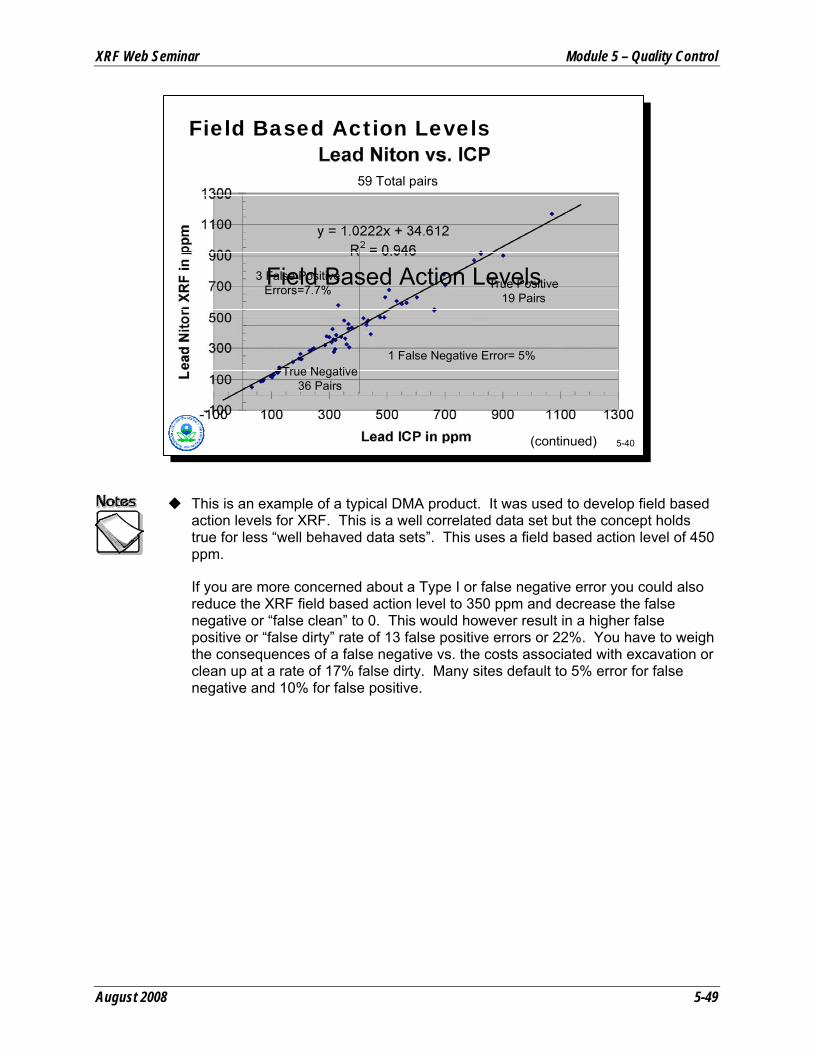
This is an example of a typical DMA product. It was used to develop field based action levels for XRF. This is a well correlated data set but the concept holds true for less “well behaved data sets”. This uses a field based action level of 450 ppm.

If you are more concerned about a Type I or false negative error you could also reduce the XRF field based action level to 350 ppm and decrease the false negative or “false clean” to 0. This would however result in a higher false positive or “false dirty” rate of 13 false positive errors or 22%. You have to weigh the consequences of a false negative vs. the costs associated with excavation or clean up at a rate of 17% false dirty. Many sites default to 5% error for false negative and 10% for false positive.

1 False Negative Error= 5%

3 False Positive Errors=7.7%

59 Total pairs

True Positive 19 Pairs

True Negative 36 Pairs

5-40

Field Based Action Levels


(continued)


5-50 August 2008

If there is greater concern about a Type I or false negative error, the action level could be reduced to 350 ppm, which decreases the false negative or “false clean” to 0. This would however result in a higher false positive or “false dirty” rate of 13 false positive errors or 22%. The project team would have to weigh the consequences of a false negative vs. the costs associated with excavation or clean up at a rate of 17% false dirty. Many sites default to 5% error for false negative and 10% for false positive.

59 Total pairs

10 False Positive Errors= 26% True Positive

20 Pairs

True Negative 29 Pairs

0 False Negative Error= 0%

5-41


(continued)


August 2008 5-51

This slide shows the structure of a 3 way decision. There are 19 true positives, 26 true negatives, 3 false positives, and 11 samples for ICP. The region of uncertainty is 350-450 ppm. Below 350 is definitely clean, above 450 is definitely dirty (with 5% false positives).

3 False Positive Errors=7.7%

59 Total pairs

True Positive 19 Pairs

0 False Negative Error= 0%True Negative 26 Pairs

11 Samples for ICP

3 Way Decision Structure With Region of Uncertainty

5-42



5-52 August 2008

5-43

Questions?

xrf and appropriate quality control - clu-in.org

Documents