yarkovsky effect on small near-earth asteroids

Icarus148, 118–138 (2000)

doi:10.1006/icar.2000.6469, available online at http://www.idealibrary.com on

Yarkovsky Effect on Small Near-Earth Asteroids: MathematicalFormulation and Examples

D. Vokrouhlicky

Institute of Astronomy, Charles University, V Holesovickach 2, CZ-18000 Prague 8, Czech Republic

A. Milani

Dipartimento di Matematica, Universita di Pisa, Via Buonarroti, I-56127 Pisa, Italy

and

S. R. Chesley

Jet Propulsion Laboratory, California Institute of Technology, Pasadena, California 91109E-mail: [email protected]

Received March 13, 2000; revised May 31, 2000

The Yarkovsky effect is a subtle nongravitational phenomenonrelated to the anisotropic thermal emission of Solar System objects.Its importance has been recently demonstrated in relation to thetransport of material from the main asteroid belt (both to explainthe origin of near-Earth asteroids and some properties of meteorites)and also in relation to the aging processes of the asteroid families.However, unlike the case of the artificial satellites, the Yarkovskyeffect has never been measured or detected in the motion of naturalbodies in the Solar System. In this paper, we investigate the possi-bility of detecting the Yarkovsky effect via precise orbit determina-tion of near-Earth asteroids. Such a detection is feasible only withthe existence of precise radar astrometry at multiple apparitions.Since the observability of the Yarkovsky perturbation accumulatesquadratically with time the time span between radar observations isa critical factor. Though the current data do not clearly indicate theYarkovsky effect in the motion of these bodies, we predict that thenext apparition of several asteroids (in particular, 6489 Golevka,1620 Geographos, and possibly 1566 Icarus) might reveal its ex-istence. Moreover, we show that the Yarkovsky effect may play avery important role in the orbit determination of small, but stillobservable, bodies like 1998 KY26. If carefully followed, this bodymay serve as a superb probe of the Yarkovsky effect in its next closeapproach to the Earth in June 2024. c© 2000 Academic Press

Key Words: asteroids; Yarkovsky effect; orbit determination.

1. INTRODUCTION AND MOTIVATIONS

eo

h

dynamical lifetime. However, besides this short-range gravita-tional interaction with terrestrial planets there might be addi-

ngthen-llyec-

hey-

all5 m;ctceds)

lvedser-ionsith

ratef the

re-s theallypa-

delface

ethetheeir

1

The orbital dynamics of near-Earth objects (NEOs) revmany complex problems. Among them, the influence of clplanetary encounters has been extensively studied and renized to be a principal reason for their strong chaoticity and s

1

0019-1035/00 $35.00Copyright c© 2000 by Academic PressAll rights of reproduction in any form reserved.

alsecog-ort

tional dynamical effects that increase the difficulty of modelithe NEO dynamics. The purpose of this paper is to analyzeinfluence on NEO motion of the Yarkovsky effect, a subtle nogravitational perturbation due to a recoil force of anisotropicaemitted thermal radiation of a rotating body. Since the persptive of our effort is to consider a possible observability of tYarkovsky effect, we shall not investigate its role on the dnamical lifetime of NEO orbits nor its influence on very smNEOs (e.g., the meteorite precursors of a typical size 0.5 tosee, e.g., Vokrouhlick´y and Farinella 2000). We rather restriour analysis to understanding the orbital perturbation induby the Yarkovsky effect for the near-Earth asteroids (NEAobserved at-present. Obviously, the short time scale invo('years) must be compensated by very high precision obvations. Fortunately, we have available the radar observatof about 50 NEAs, some of which have been observed wradar even during two apparitions. We intend to demonstthat data of such a superb quality may reveal the influence oYarkovsky effect on several NEA orbits.

The plan of the paper is as follows: in Section 2 we brieflycall the physical essence of the Yarkovsky effect and discusmathematical approach that will be used. Though we basicput together previous results, new results presented in thisper include the definition of algorithms to determine the moparameters of the diurnal Yarkovsky acceleration (the surthermal conductivity and the orientation of its spin axis). Wshall also point out that modeling of the Yarkovsky effect onNEA orbits presents a special problem not encountered insimilar orbital analysis of the main-belt objects, and that is th

8

A

ut

n

u

tee

rlet/ti

u

de

t

tit

atg

z

n

,gg

t

ar-7).c-te

uralld

ted-

eenama-noos-

ssesdel

l-ore

cethes ais aenuxbyndncyeirleofcter-

se-hear asetryce

ove,ionts

ast

-tionarecytiontyp-

ceto

YARKOVSKY EFFECT ON SM

high eccentricity. Then, in Section 3, we determine the secsemimajor axis drift (the main orbit perturbation) caused byYarkovsky effect for selected, known NEAs and we estimausing simple analytical formulas, a characteristic orbital chaproduced by this effect. These results offer a first glimpsea more complete understanding of the way the Yarkovskyfect affects NEA orbits. We shall also consider how the resdepend on the value of the surface thermal conductivity ofasteroid, which is a particularly important issue in the conof this paper. However, the detection of the Yarkovsky effvia NEA observations and orbit determination requires alsdetailed consideration of both observational and orbit detenation errors. The observation errors are small enough to afor the detection of the Yarkovsky effect, since the present prsion of the radar ranging technology is on the level of a fracof a microsecond or about 60 m in range and about 100 min the range–rate measurement. However, the global orbitermination uncertainty must be considered, and it substantexcludes the possibility of detection of the nongravitational pturbations within the currently available data. We then discwhich additional observations would be sufficient for this dtection, and find some very interesting possibilities for the nfew years. We devote Section 4 to this topic.

2. YARKOVSKY EFFECT: THE SPLIT ONTO DIURNALAND SEASONAL VARIANTS

The applications of the Yarkovsky effect in Solar Systemnamics have undergone a remarkable renaissance over thfew years. This situation results from a fruitful conjunctionprogress in several fields. On one side, the classical undersing of the Yarkovsky effect has been enlarged by a moretailed theoretical analysis that finally resulted in the recogniof the mean-motion mode of the thermal effect (now called“seasonal” variant of the Yarkovsky effect; see, e.g., Rubinc1995, 1998; Farinellaet al.1998; and herein). On the observtional side, direct and indirect knowledge of the dynamics ofsmall Solar System bodies has dramatically increased durinpast few years. Here we have in mind the systematic searcheNEOs with powerful CCD systems, the previously mentionradar ranging to NEAs and also more detailed and precise msurements of the cosmic-ray exposure ages of meteorites (wprovide indirect evidence of the transfer time from the mainteroid belt toward the Earth; e.g., Graf and Marti 1995, Heret al.1997).

Although the role of Yarkovsky perturbation has been recediscussed in relation to meteorite properties (e.g., Farinellaet al.1998, Hartmannet al. 1999, Vokrouhlický and Farinella 2000Bottke et al. 2000), the replenishment of large NEAs (e.Farinella and Vokrouhlický 1999), and asteroid family aginprocesses (e.g., Farinella and Vokrouhlický 1999, Vokrouhlickýet al. 2000), so far there has not been any direct measuremof the Yarkovsky perturbation in the orbital motion of the na
ral bodies in the Solar System (despite extensiveobservational
LL NEAR-EARTH ASTEROIDS 119

larhete,geofef-lts

thextct

o ami-lowci-

iondayde-allyer-ss

e-ext

y-past

ofand-de-onheam-hethe

s foredea-

hichas-og

tly

.,

entu-

evidence of the Yarkovsky effect in the case of the motion oftificial Earth satellites such as LAGEOS, e.g., Rubincam 198Although the Yarkovsky effect is unavoidable from the perspetive of physical principles, its direct measurement might validathe available (and necessarily approximate) models for natbodies like asteroids and their fragments. In this way it woualso enhance the credibility of the other ongoing work relato the Yarkovsky effect. This line of thinking is a principal motivation of the present work.

It is also worth mentioning that the orbit analysis of somNEAs has suggested evidence of nongravitational phenomby requiring an anomalous secular decrease of their semijor axis (e.g., Sitarski 1992, 1998). At that stage of analysisprecise physical mechanism was mentioned apart from a psible, but vague, reference to outgassing, comet-like proce(conformal to using the classical empiric approach to mothe nongravitational effects on cometary orbits:apert' (a/2a) v;Sitarski 1998). Involving the Yarkovsky effect in the orbit anaysis of these cases might offer an additional and perhaps msophisticated approach.

As mentioned above, the Yarkovsky effect is a recoil forfrom the thermal radiation of cosmic bodies that accumulateenergy by absorbing solar radiation in the optical band. Aresult, an anisotropic distribution of the surface temperaturenecessary condition for a nonzero Yarkovsky force. For a givsurface element of the body, the incoming solar radiation flin the body-fixed reference frame is essentially modulatedtwo frequencies: (i) the rotation frequency of the body arouan instantaneous spin axis and (ii) the mean-motion frequethat is given by the body’s revolution around the Sun (plus thmultiples and linear combinations). In the context of a simp(linearized) heat diffusion theory the temperature variationthe surface element basically keeps the same spectral charaistic with one exception: the individual spectral lines are phashifted in a precisely determined way. When performing tinverse Fourier map these phase shifts obviously then appetime lags. Taking into account the assumed spherical geomof the body and the individual temperature history of the surfaelements, computed according to the theory mentioned abwe may determine the net recoil force of the thermal radiat(by performing a surface integration of the infinitesimal effecon the sphere).

Theoretical reanalysis of the Yarkovsky effect over the pfew years (e.g., Rubincam 1995, 1998; Farinellaet al. 1998;Vokrouhlicky 1998a,b, 1999) has revealed the following important results. The surface-integrated Yarkovsky acceleraterms that depend on the rotation frequency of the bodytightly clustered around the spectral line with this frequen(showing up as mean-motion sidebands) and yield acceleracomponents perpendicular to the spin axis. Thanks to theically big difference between the periods of rotation (≈hours)and revolution (≈years), these acceleration terms in practi“collapse” to the single spectral line corresponding simply
the rotation frequency. Another aspect of the same reasoning

emdh

th

tuefet

kx

ehnte

li

n

sae

)

kvgto

n

s

hesizeler-

heem-rtial

u-delthexity.n byza-las

er-) thesan-sti-itemmsu-

tatis;arusa-

-tionene-notfor

tionenher-f thetiony).(asut

cope

rit-

ti-

120 VOKROUHLICKY, MIL

comes from the fact that the thermal relaxation time scale cosponding to the rotation frequency of the body (approximatthe time between the sunlight absorption and the thermal esion) is comparable to the rotation period, and thus the boshift along the orbit around the Sun may be neglected. Wthese force components are transformed to the inertial reence frame, to which the orbital perturbations are referred,have close to zero frequency with amplitude still dependingthe rotation rate of the body. Because of their relation torotation period the acceleration terms mentioned above areally called “diurnal.” Their modeling is sufficiently simple sincthey depend uniquely on the instantaneous state vector obody in its orbit. In particular, the eccentricity of the orbit donot enter the computation of the diurnal Yarkovsky acceleracomponents at this level of approximation. However, in his pneering work, Rubincam (1995, but see also his related worsatellite dynamics, Rubincam 1987) has shown that there eanother class of thermal acceleration terms, computed bysurface integration mentioned in the previous paragraph, thanot depend on the rotation frequency of the body but only onrevolution frequency around the Sun (and its multiples). Thterms, usually called “seasonal” because of their frequency cacteristics, are always aligned with the body’s spin axis. Siwe assume a fixed orientation of the spin axis in the inerspace, the seasonal component of the Yarkovsky force presits revolution frequency even in the inertial frame. If describedan approximate way, the seasonal acceleration terms are reto the changing geometry of the north/south hemisphere instion of the body. Each of these two effects, diurnal and seasomay be important in the dynamics of small cosmic bodiesNEAs.

Keeping the terminological and practical split into the diunal and seasonal variants of the Yarkovsky effect mentioabove, we shall summarize our mathematical approach inremainder of this section. In the case of the diurnal variantshall essentially follow the approach developed by Vokrouhlicy(1998a). The necessary formulas are given in Section 2.1the partials with respect to the most important parameterscomputed analytically. The seasonal variant of the Yarkoveffect deserves more attention since it hides more complicproblems. The latter arise mainly because of high orbitalcentricities (which can range from 0.3 up to very “extreme,”cometary-like values, e.g.,' 0.823 in the case of 1566 Icarusso that the analytic evaluation of the incoming solar radiation flbecomes troublesome. On top of this difficulty, Vokrouhlicyand Farinella (1998) have pointed out another problem in euating the seasonal component of the thermal force. For hieccentric orbits the variations of temperature along the orbiparticular over a thermal relaxation time scale of the seaseffect, are large enough so that the basic assumptions ofearization of the heat diffusion problem are violated. Avoidithe linearization approach yields a precise result, but requa completely numerical solution. In what follows, we shall uthe model of Vokrouhlický and Farinella (1998), which solve
the thermal state of the body along an arbitrarily eccentric
ANI, AND CHESLEY

rre-lyis-

y’sen

fer-ey

onhesu-

thes

ionio-oniststhet doitssear-ceialrvesin

latedola-nal,ke

r-edthewekándarekytedc-

,uxál-hly, innallin-g

iresse

bit in the “large-body” approximation (penetration depth of tseasonal thermal wave is much smaller than the geometricof the body). The amplitude of the seasonal Yarkovsky acceation is then formally given in terms of an integral in which tintegrand contains the latitude stratification of the surface tperature. The latter, in turn, results from a solution of a padifferential heat-diffusion equation. The corresponding formlas are outlined in Section 2.2.2. Though precise, this mofor the seasonal Yarkovsky force may not be well suited forroutine orbit determination process because of its compleWe thus also consider a less precise, but analytical solutioVokrouhlicky and Farinella (1999), which is based on linearition of the heat diffusion problem. The corresponding formuare outlined in Section 2.2.1.

2.1. Yarkovsky Diurnal Acceleration

There are two basic assumptions of the Vokrouhlický (1998a)model of the diurnal variant of the Yarkovsky effect: (i) tempature throughout the body is close to a mean value, and (iibody is spherical (with radiusR). The first of these two itemallows linearization of the heat diffusion problem and, thus,alyticity of the solution. Since the thermal relaxation time, emated above, is not much shorter than the rotation period,(i) might be a fairly good approximation. The second ite(ii) might present an obstacle for small NEAs, since they are ually of a rather irregular shape (e.g., Ostroet al.1996, 1999a forthe most extreme cases of 1620 Geographos and 4179 Tousome are fortunately less-elongated objects, like 1566 Icwith the following ratio of the dimension along the inertimoment principal axesa/b = 1.23± 0.04 andb/c = 1.40±0.10, e.g., De Angelis 1995). Vokrouhlický (1998b) has developed a theory for computing the diurnal Yarkovsky acceleraon spheroidal objects (whose size is much larger than the ptration depth of the diurnal thermal wave), but his results areeasily incorporated into numerical integrations, especiallythe nonprincipal axis rotators; moreover, their generalizafor triaxial bodies would only increase the complexity. Givthe substantial uncertainty in our knowledge of the surface tmal parameters, we believe that errors incurred by the use ospherical assumption may be partly aliased into the estimaof the surface conductivity (or the effective size of the bodTailoring the thermal model for a given shape of an asteroidis typical in the case of artificial satellites) will probably turn oto be necessary in the future, but this topic is beyond the sof this paper.

The diurnal variant of the Yarkovsky acceleration can be wten in the form (see also Broˇz et al.2000)

ad = 4α

9

8(r )

1+ λG[sinδ + cosδs×]r × s

r, (1)

whereα is the absorptivity of the asteroid surface in the opcal band (complementary to albedo),s is the unit vector of the

or-spin axis, andr is the heliocentric position vector (r = |r |). The

A

i

t

r

v

en-

´

.

r-)

tedldkyem

rbitt-

ctslting

d onondur-erthe

tc.)

ky

n

A′(x) = d A(x) = −1+ ex[cosx + (2x − 1) sinx], (13)


standard radiation force factor8 is defined by

8(r ) = 3F(r )

4Rρc, (2)

with F(r ) being the solar radiation flux at the instantaneodistancer from the Sun (henceF(r ) ∝ 1/r 2), c the speed oflight, andρ the mean density of the fragment. The instantanesolar radiation fluxF(r ) determines the local (in terms of thorbital revolution) subsolar temperatureT(r ) through

εσT4(r ) = αF(r ), (3)

with σ being the Stefan–Boltzmann constant. The subsolar tperature defines the diurnal thermal parameter2 = √KρsCω/εσT3(r ) and the local value of the penetration depth of the dnal thermal waveld =

√K/ρsCω. HereK is the thermal con-

ductivity, C is the thermal capacity,ω is the rotation frequencyandρs is the surface density. In principle, this latter quantmay not be identical to the mean bulk densityρ from Eq. (2).The argumentX in Eq. (4) isX = √2 R/ ld and the parameteλ is defined byλ = 2/X.

Finally, the amplitudeG and the phaseδ in Eq. (1) are givenby

Gei δ = A(X)+ i B(X)

C(X)+ i D(X), (4)

(i = √−1 is the complex unit) with the auxiliary functions

A(x) = −(x + 2)− ex[(x − 2) cosx − x sinx], (5)

B(x) = −x − ex[x cosx + (x − 2) sinx], (6)

C(x) = A(x)+ λ

1+ λ {3(x + 2)+ ex[3(x − 2) cosx

+ x(x − 3) sinx]}, (7)

D(x) = B(x)+ λ

1+ λ {x(x + 3)− ex[x(x − 3) cosx

− 3(x − 2) sinx]}. (8)

A few remarks are in order to illuminate the features ofdiurnal acceleration (1).

• Note that the diurnal acceleration (1) is perpendiculathe body’s spin axis (ad · s= 0). The along-spin acceleratiocomponent is then given by the seasonal variant of the Yarkoeffect and it will be discussed below.• For future use we introduce functionsa(x) andb(x) by the

formulas

C(x) = A(x)+ λ

1+ λa(x) and D(x) = B(x)+ λ

1+ λb(x).

• As a reference check of the numerical simulations, we m
tion here the analytical estimation of the semimajor axis drift d

us

ouse

em-

ur-

,ity

r

he

tonsky

to the diurnal variant of the Yarkovsky effect (e.g., Vokrouhlicky1998a, 1999)

da

dt= −8α

9n8(a)

G sinδ

1+ λ cosγ +O(e) (9)

(8(a) = 8(r = a) since (9) is correct for the circular orbit only)Here,n is the mean motion andγ is the obliquity of the body’sspin axis. Numerical tests indicate that for high eccentricity obits (like 1566 Icarus,e' 0.827) the approximate result (9should be increased by a factor of 1–5.

Some of the Yarkovsky effect parameters might be adjusin the orbit determination procedure. For this goal we wouneed to calculate partial derivatives of the diurnal Yarkovsacceleration (1) with respect to those parameters. Some of thare given below.

Since the surface thermal conductivityK is the principal un-known parameter of the thermal model outlined above, the odetermination should focus on fitting this parameter. Anticipaing the results of this paper, we note that the NEA orbits/objecan have either a weak or a strong dependence of the resuorbital perturbations on the surface conductivityK . Both casescan be interesting. In the first case the results do not depena badly constrained parameter in the model, while in the seccase we might wish to determine, or at least constrain, the sface conductivity value. We recall that knowledge of the lattmight have imposed constraints on the physical character ofsurface (degree of particularization, existence of regolith, ethat, in turn, has cosmogonic implications.

The corresponding partial derivative of the diurnal Yarkovsacceleration (1) is

K∂K (ad) = 4α

98(r )

{K∂K

(G sinδ

1+ λ)

+ K∂K

(G cosδ

1+ λ)

s×}

r × sr

(10)

(∂K = ∂/∂K ). The partial derivatives on the right-hand side cabe determined from the relation

K∂K

{G expi δ

1+ λ}= −G expi δ

1+ λ ξK , (11)

where the complex factorξK is given by

ξK = λ

1+ λ

×{

1+ X

2

[ A′(X)+ i B ′(X)][a(X)+ ib(X)]− [ A(X)+ i B(X)][a′(X)+ ib′(X)]

[ A(X)+ i B(X)][C(X)+ i D(X)]

}.

(12)

Here we have used the derivatives

ue dx

L

e

e

t

o

ce

ee

d

g

c

f

enur-

tionst-nds

mal

or

erof

noties

xi-ysap-cet

n.aleut

istsn.gh-e-

the

122 VOKROUHLICKY, MI

B′(x) = d B(x)

dx= −1− ex[(2x − 1) cosx − sinx], (14)

a′(x) = da(x)

dx= 3+ ex[(x2− 3) cosx

+ (x2− 4x + 3) sinx], (15)

b′(x) = db(x)

dx= 2x + 3− ex[(x2− 4x + 3) cosx

− (x2− 3) sinx]. (16)

In general, the thermal conductivityK , and to a lesser extenthe thermal capacityC and the densityρ, are functions of thetemperature. A higher mean temperature results in the methe surface particles to a larger matrix that enables more efficconduction, but decreases the role of the intergrain radiatransport. Given such physical concepts of the heat transpothe surface material, several parametrizations of theK vs T de-pendency were theoretically proposed and experimentally te(e.g., Wesselink 1948, Glegget al.1966, Wechsleret al.1972).However, given the other simplifications of our approachshall neglect the temperature dependence of the thermal mparameters in this paper.

As mentioned above, the asteroids that we have selectour study for a possible measurement of the Yarkovsky efwere all observed with radar technology. These were selein order to obtain the highest precision of orbital data. Modradar measurements allow the capability of determining bothorbit (“center-of-mass” position and motion) and the shapethe asteroid. This is, for instance, the case with 4179 Tou(Ostroet al.1999a), 1620 Geographos (Ostroet al.1996), and6489 Golevka (Hudsonet al.2000). The objects are generallya rather irregular shape, which is conventionally approximaby a triaxial ellipsoid. Since our model for the Yarkovsky forassumes a spherical body, we shall determine its effectivdius R by an “equal-mass-condition,”R3 = abc, wherea, b,andc are radii along the principal axis of the ellipsoid modIn some other cases, however, we have much less reliablformation about the size of the body. For instance Veederet al.(1989) report the radiusR= 450 m for 1566 Icarus provideits albedo is about 0.4. This albedo, however, seems to be qularge, and Harris (1998) advocated a larger size for this asteand a correspondingly smaller optical albedo. In a recent paMahapatraet al.(1999) however seem to indicate that the orinal solution of small-size Icarus might be correct. (This issucarefully considered in Section 3.3.)

In these latter cases especially, it might be interesting tostrain the radiusR of the body via the orbital perturbation othe Yarkovsky thermal effect. In other words, solving for tformal, Yarkovsky-determined radius of the body, we may again insight into the reliability of the Yarkovsky model for thparticular body. To that end we need the partial derivatives oYarkovsky acceleration with respect to the radius of the bo
The resulting formula is rather simple and, moreover, does
ANI, AND CHESLEY

t

ltingienttionrt in

sted

weodel

d infectctedrntheof

atis

ftedera-

l.in-

iteroidper,i-

e is

on-f

helsoisthedy.

demand supplementary computational expense

R∂R(ad) = −1+ 2λ

1+ λ ad− 2K∂K (ad), (17)

where the derivative in the last right-hand-side term is givin (10) and was thus already computed. Obviously, both sface thermal conductivityK and the radiusR of the body affectthe semimajor axis change. Their simultaneous determinawould not be possible. However, the situation might be intereing in several cases where the semimajor axis mobility depelittle on theK value (see Section 3 below).

2.2. Yarkovsky Seasonal Acceleration

As explained above, the seasonal component of the therYarkovsky acceleration is collinear with the orientationsof thespin axis, hence,

as = fZs . (18)

Vokrouhlicky (1999) obtained a simple analytic expression ffZ that is, however, only valid for circular orbits, whileVokrouhlicky and Farinella (1999) obtained a solution for thfZ amplitude in terms of elliptic series that is formally valid foeccentric orbits. Both solutions are based on the linearizationthe heat diffusion problem on a spherical body and, thus, canbe fully precise. Obviously, the convergence of the elliptic-sersolution of Vokrouhlicky and Farinella (1999) is violated in thecase of highly eccentric orbits (e.g., 1566 Icarus), so appromating the series by the first few terms, as we practically alwamust do, may produce misleading results. The only preciseproach then is a completely numerical solution. However, sinthis solution is computationally very difficult, we shall adoptwo possible options for the seasonal Yarkovsky acceleratio

The first, “lower precision” solution is based on the analyticresults of Vokrouhlick´y and Farinella (1999). Our experiencshows that it can be used up to eccentricity of 0.4–0.5 withoa major corruption of the results. Its main advantage consof its analyticity and thus high speed of numerical evaluatioFor special cases of very eccentric orbits we shall use the “hiprecision,” numerical solution. Both approaches are briefly dscribed in the following two paragraphs.

2.2.1. The low-precision model.At a lower precision ofmodeling the seasonal Yarkovsky effect we have adoptedlinearized solution by Vokrouhlick´y and Farinella (1999). Theacceleration amplitudefZ from (18) then takes the form (formore details see Broˇz et al.2000)

fZ = 2α

9

8(a)

1+ λ′∑k 6=0

χkGkei δkζ k. (19)

Here,λ′ = λ η3/4 (η = √1− e2). In principle, the summation in
not(19) is to be performed over all integer and nonzero values ofk;

A

T

o;t

e

o

e

t(

-lly

era-er-

naryr

nallsoentforly-

theost

ef-the

at


however, in our program we restrict to|k| < 8. This is justifiedfor low-eccentricity orbits, since theχk factors decay fast withincreasing value of the indexk. In quantitative terms

χk ≡ sPαk − isQβk ∝ ek−1, (20)

with ebeing the eccentricity. Obviously, the convergence ofseries (19) is not guaranteed for high values of eccentricity.is the principal caution behind using the lower-precision mofor evaluation of the seasonal Yarkovsky acceleration.

VariablessP andsQ stand for projection of the spin vects onto the orbit-defined unit vectorsP (direction of pericentersP = s · P) andQ = N× P (with N being normal to the orbiplane;sQ = s ·Q). The eccentricitye dependent functionsαk

andβk read

αk = 2d

de[ Jk(ke)], (21)

βk = 2η

ek Jk(ke), (22)

whereJk(x) are the ordinary Bessel functions of the first ordExplicit expressions of the first seven coefficientsαk andβk canbe found, for instance, in Brouwer and Clemence (1961).

The thermal characteristics of the seasonal effect are exprby the amplitudesGk and phasesδk given by

Gkei δk = A(Xk)+ i B(Xk)

C(Xk)+ i D(Xk), (23)

where we assumek ≥ 1. Terms with the negative value of thindex k are obtained by the identityG−k expi δ−k = Gke−i δk .Thek-indexed arguments on the right-hand side of (23) areXk =√

2k R/ ls, with the radiusRof the body scaled by the penetratidepthls of the seasonal thermal wavels =

√K/ρCn, and the

functionsA, B, C, andD are defined by Eqs. (5) to (8) abovFinally, the complex quantityζ in Eq. (19) denotesζ = expi `,where` is the mean anomaly.

Notice that the structure of the acceleration (19) is very simto that of the diurnal effect in (1). For an evaluation of the parderivatives, with respect to the surface thermal conductivityK )and the radius (R) of the body, we may straightforwardly usthe formulas given in the previous Section 2.1.1. Obviously,seasonal-effect-related variables, e.g., scaling the radius obody by the penetration depth of the seasonal thermal wavls,must be used. In particular, the partial derivative of thefZ ampli-tude with respect to the surface conductivityK reads (comparewith Eq. (10))

K∂K { fZ} = −2α 8(a) ∑χkGkei δkξ k ζ k, (24)

9 1+ λ′k 6=0

K


thehis

del

r

er.

ssed

e

n

.

ilarial

ethef thee

where the complex factorsξ kK are

ξ kK =

λ′

1+ λ′

×{

1+ Xk

2

[ A′(Xk)± i B ′(Xk)][a(Xk)± ib(Xk)]− [ A(Xk)± i B(Xk)][a′(Xk)± ib′(Xk)]

[ A(Xk)± i B(Xk)][C(Xk)± i D(Xk)]

}(25)

(the minus signs are for negative values of the indexk). Similarlythe partial derivative with respect to the radiusR of the body isgiven by

R∂R(as) = −1+ 2λ′

1+ λ′ as− 2K∂K (ss), (26)

which is identical (apart from the changeλ→ λ′) to Eq. (17).

2.2.2. The high-precision model.In the case of orbits obeying a very high eccentricity, we shall use a nonlinearized, funumerical model developed by Vokrouhlick´y and Farinella(1998). Then the amplitudefZ from (18) is formally given asan integral over all latitudesθ on the body

fZ = −4α

38a

∫ 1

−1d(cosθ ) cosθT ′4(θ ), (27)

with8a = πR2F(a)/mcandF(a) being the radiation flux at thesemimajor axis distance from the center as before. The temptureT ′ in the integrand of (27) is scaled by the subsolar tempature at “the semimajor axis distance,” i.e.,εσT4

a,? = αF(a). Itslatitudinal distributionT ′(θ ) results from a numerical solutioof the 1-D heat diffusion equation with an appropriate boundcondition (see Vokrouhlick´y and Farinella 1998). Hence, oucode first computes numericallyT ′(θ ) at any instant along theorbit (of any eccentricity) and then computesfZ by numericalquadrature (27).

Since the implementation of the high-precision seasoYarkovsky acceleration is completely numerical, we must acompute the partials by the finite difference method. To prevnumerical errors while computing the seasonal accelerationtwo close values of the parameter for which we anticipate ponomial dependence (thermal conductivityK and radiusR) wemay use

∂ fZ

∂K= 1

K

∂ fZ

∂ ln K(28)

and similarly for the radiusR.

3. THE FIRST GLIMPSE: SEMIMAJOR AXIS MOBILITYOF NEAs AND TESTS

In this section, we shall compute the expected drift ofsemimajor axis for selected asteroids that might be the mpromising candidates for determination of the Yarkovskyfect. Note that the secular change of the semimajor axis isprincipal indicator of the Yarkovsky orbital perturbation th
can lead to observable effects (the perturbation of the other

der

use

124 VOKROUHLICKY, MILANI, AND CHESLEY

TABLE ICandidate Asteroids for Detection of Yarkovsky Effect

Spin axis orientation parameters (◦)

Asteroid a (AU) R (km) P (h) ` b γ Ref.

1566 Icarusa 1.08 0.45 2.273 214 5 103 1, 21620 Geographosb,c 1.25 1.21 5.225 56 −47 150 3, 4, 51685 Toro 1.37 1.7 10.19 210 40 41 1, 24179 Toutatisb,d 2.51 2.76 6.93 180 −52 143 46489 Golevkab 2.51 0.27 6.03 202 −45 134 61998 KY26e 1.23 0.015 0.17837 — — 0(180)? 7

Note.For each of the objects we give the semimajor axisa (in AU), radiusR (in km), rotation periodP (in hours), the ecliptic longitude and latitude (`, b) ofthe spin axis orientation, and its obliquityγ . The obliquity is helpful in getting an idea of which of the variants of the Yarkovsky effect dominates;γ ' 90◦ meansthe seasonal variant is dominant,γ ' 0(180)◦ means the diurnal variant is dominant. Source references are listed in the last column. References: (1) Veeet al.(1989); (2) De Angelis (1995); (3) Ostroet al. (1996); (4) Ostroet al. (1999a); (5) Magnussonet al. (1997); (6) Hudsonet al. (2000); (7) Ostroet al. (1999b).

a The quoted radius has been reported by Veederet al. (1989). However, since these authors have used a rather high value of the albedo (0.4), the 0.45-kmradius of 1566 Icarus may be just the lower estimate. In this context, note the test we have performed in Section 3.3. For the spin axis orientation wedata byDe Angelis (1995), whose analysis discarded the ambiguity in the sense of orientation of the Icarus spin axis.

b A triaxial model has been determined from radar observations, and we have estimated an “effective radius” byR3 ' abc, wherea, b, andc are the dimensionsalong the principal axis of the moment of inertia.

c Spin axis orientation by Magnussonet al. (1997).d We approximate the “spin axis orientation” by the direction along the angular momentum vector.e This is one of the smallest objects observed so far by the radar technique. (Its smallness obviously favors the influence of the Yarkovsky effects.) Theobservations

of 1998 KY26 might indicate the spin axis nearly perpendicular to the ecliptic plane (without possibility of resolving the sense of rotation; P. Pravec, personalcommunication).

io

eotm

atee

m

oe

ewta

t

heely.nts

xiste.oid

e-tht-on-xise-

this

f-

ra-

is-the

elements are less important except, perhaps, the inclinatAs far as the “candidate bodies” are concerned we havelected the asteroids that had been observed by radar at twmore apparitions (according to the list given athttp://ssd.

jpl.nasa.gov/radar data.html ). These are generally thbest known orbits among the NEAs. A list of the selected bies is given in Table I, where the assumed size and rotaparameters are also indicated. As far as the orbital paraters are concerned we used theOrbFit software, developedby the OrbFit Consortium (seehttp://newton.dm.unipi.it/

˜asteroid/orbfit/ ), which enables precise orbit determintion (including radar observation processing). A check withindependent JPL solutions for individual objects has also bperformed (e.g., Ostroet al. (1999a) for 4179 Toutatis). Sincdetailed information about the surface properties of thesejects is usually not available, we shall span the surface therproperties (in particular, the thermal conductivityK ) in somephysically reasonable range. The absorption coefficientα in theoptical band is typically 0.9 (corresponding thus to an albedo0.1), but in specific cases we accept the published values (the case of Icarus and Golevka). The emission coefficientε inthe thermal band is always set to 0.9.

The integrations performed in this section represent a pturbed two-body problem; i.e., no planetary effects have bincluded. This is already a fairly good approximation sincedo not expect any significant coupling between the planeand Yarkovsky perturbations. However, in Section 4 we shproceed with a full numerical simulation involving a comple
model for the orbit determination (including planetary perturb
n).se-o or

d-ion

e-

-heen

ob-al

f.g.,

er-enery

alle

tion and general relativity effects). We consider the effect of tdiurnal and seasonal variants of the Yarkovsky effect separatThe total effect is then a simple superposition of the two variaat this level of approximation.

To understand how the computed drift in the semimajor atranslates into an orbital shift we perform the following estimaThe principal effect consists of a quadratic term in the asteranomaly on the order1M ' − 3

4n(da/dt)(1t)2/a, wheren isthe mean motion,da/dt the estimated semimajor axis drift duto the Yarkovsky effects,1t the elapsed time between two observations, anda the semimajor axis. This effect produces botransverse displacement1τ ' aη1M and a radial displacemen1r ' ae1M/η with η = √1− e2 (see, e.g., Casotto 1992; notice that the radial displacement is to be dominated by the lgitudinal term rather than by a change in the semimajor asince the former effect is quadratic in time). The total displacment thus reads1ρ ' a1M , where the fourth-order terms ineccentricity have been neglected. In terms of physical unitsmeans

1ρ ' 7a4(110t)2a−3/2

AU km, (29)

wherea4 is the Yarkovsky drift of the semimajor axis in 10−4 AU/Myr (this is a typical order of magnitude of the Yarkovsky efects on the near-Earth objects; see below),110t is the timedifference in tens of years (a characteristic temporal sepation of two “radar apparitions”), andaAU is the semimajor axisin astronomical units. We should mention that the actual dplacement of the asteroid with respect to the radar station of
a-Earth then depends on a particular Earth–asteroid geometry. This

la

tod

h

t

to

oi

c

tlye

s

hatr-

g ofectsthat

cts)ity

jorf the

ionnal

di-es.en

heka)Onn re-di-

ch

ighto arnalheces as

theortherjor-nts.lvedcal,ima-ingthus

YARKOVSKY EFFECT ON SMA

effect may partly decrease the estimated value of1ρ from (29),though not by orders of magnitude. We shall check this clain Section 4 where we shall perform a full numerical simution of the objects’ displacement in their future apparitions.the case of some NEAs we have a rather long series of opobservations (e.g., 1566 Icarus) or prediscovery identificati(e.g., 4179 Toutatis). Then, we also express the longitudeplacement1M directly:

1M ' 0.01′′a4(110t)2a−5/2

AU . (30)

As the small NEAs are often observed at close approachethe Earth only, this change in the mean anomaly may then ima sky displacement (usually in the right ascension) given1M × (a/rmin), wherermin is the minimum distance to the Eartat the approach. The latter factor can sometimes result in a faof 10–100 amplification of (30).

In what follows we shall assume the nominal estimates ofradii (given in Table I). We have checked that the semimajor adrift due to the Yarkovsky effects scales as∝R−1 for objects ofsizes larger than about 20 m (see, e.g., Farinellaet al.1998), acondition that applies for all the considered cases.

3.1. Diurnal Yarkovsky Effect

In this section we shall deal with the diurnal variant of thYarkovsky effect. Figure 1 shows the estimated values ofsecular semimajor axis drift as a function of the surface cductivity K . If the surface is particularized (covered with thimpact-produced regolith) or has a high degree of micropority (due to the impacts of dust particles) its conductivity wbe low: 0.001–0.01 W/m/K. On the other hand, if the body ha

FIG. 1. The estimated secular drift|da/dt| of the semimajor axis due to thediurnal variant of the Yarkovsky effect for selected asteroids vs the surfaceductivity K . In the case of 1685 Toro the semimajor axis drift is positive (dashline), while in all other cases the orbits decay (da/dt negative, solid lines). Nom-
inal values of the spin axis orientation and radii (from Table I) are assumed.

im-

Inicalnsis-

s toplyby

ctor

hexis

ehen-es-

lls

on-ed

a fresh, solid surface the conductivity would be significanhigher:'1 W/m/K. A lower degree of porosity of otherwissolid rock results in the thermal conductivity of about 0.1 W/m/K(e.g., Wechsleret al. 1972, Yomogida and Matsui 1983). Thilatter case is likely for very small objects such as 1998 KY26

(radius of only 15 m), while a value of 0.01 W/m/K seems themost likely value for the larger objects in our sample. Notice tMuller et al. (1999) report typically very low values of the suface thermal conductivity ('0.001 W/m/K in our units) for thelarge main-belt asteroids from the thermophysical processinthe ISO measurements. This would indicate that these objhave regolith-like surfaces. It seems reasonable to assumethe NEA surfaces (smaller and presumably younger objemight have about a factor 10 times higher thermal conductivas mentioned above.

We note that the diurnal effect may result in both semimaaxis increase and decrease, depending on the obliquity ospin axis. In one case (1685 Toro) we have foundda/dt to bepositive (dashed line in Fig. 1), while in all other casesda/dt isnegative (solid lines in Fig. 1). In the former case the contributof the seasonal Yarkovsky effect may partially cancel the diurdrift, while in the latter case it adds to the diurnal value.

The results in Fig. 1 indicate that a few times 10−4 AU/Myrare the typical values of the semimajor axis drift due to theurnal variant of the Yarkovsky effect on our sample of bodiThis order of magnitude fits well the previous estimates givby Farinellaet al.(1998) or Bottkeet al.(2000). There are both“obvious” and “unexpected” features in this figure. Among tobvious results we notice that smaller objects (6489 Golevexhibit higher mobility than the large ones (4179 Toutatis).the other hand, we also present results that have not beeported so far. In the case of Icarus, for instance, the higherurnal mobility appears for higher surface conductivity, whiis just opposite to the previous experience (e.g., Farinellaet al.1998). This reversal is most probably caused by the very heccentricity of the orbit. In some cases (4179 Toutatis andlesser extent also 1685 Toro and 1620 Geographos) the diumobility of the semimajor axis depends only very weakly on tsurface conductivity. This is, in fact, a favorable circumstansince this parameter is unconstrained by other observationhas been mentioned above.

The principal effects that may cause computed values ofda/dtto be uncertain are: (i) badly estimated characteristic size ofbody, (ii) nonsphericity of its shape, and (iii) badly determinednonstationary (precessing) spin axis. All these factors togemay result in a factor of 2 or 3 of mismodeling the semimaaxis drift (see, e.g., Vokrouhlick´y 1998b). As far as the characteristic size of the body is concerned we have two commeFirst, in cases where triaxial characteristics have been reso(e.g., Toutatis and Geographos) from combination of the optiinfrared, and radar observations, we have used an approxtion by a sphere of equivalent volume (see above). By doso we at least keep approximately the same volume and
mass of the body. However, in some cases the body might not be

L

p

h

d

pr

1q

uf

ymnl

i-

iaal

tis

ornof

rhered

ysnt

,,er-

y

faceconductivity K . In all cases the orbit decays. Nominal values of the spin axis


fitted well even with an ellipsoid, for instance, Toutatis (Oset al.1999b). Secondly, we recall that the semimajor axis d(da/dt) scales inverse-proportionally with the characteristicdius of the body. As a result a change in the radius affectssemimajor axis mobility in a very simple way.

Next, we comment on the issue of the spin axis orientatThe pole characteristics (longitude and latitude) are usuallytermined upto a few degrees of uncertainty (in the best casesthe contrary, in several cases (4179 Toutatis or 1620 Geograwe know the rotation state very precisely from the detailed aysis of the radar data. As expected, some bodies do not exhsimple (uniform) rotation about a spatially fixed axis but rattumble around the constant vector of the total angular momtum (as in the case of Toutatis; Ostroet al.1999b). To understanthe sensitivity of our results to changes in the orientation ofspin axis we have performed the following test. We have csidered fictitious configurations with the spin axis sweepincone with some aperture around the nominal value of theorientation (given in Table I). We have taken 2.5◦, 5◦, 7.5◦, and10◦, respectively, for the aperture angle. Fixing the value ofsurface conductivity (to 0.01 W/m/K), we have computed thsemimajor axis drift for bodies rotating about the fictitious saxes (the position of which on the cone has been parametby an angleα). No changes in the rotation period were assumThe results are shown in Figs. 2 and 3. In some cases (Geographos and 4179 Toutatis), the results from Fig. 1 arerobust on changing the spin axis orientation since theda/dt drifton even the 10◦ cone stay close to the central value. 1566 Icaand 6489 Golevka show larger sensitivity to changes in theaxis orientation. However, assuming that the spin axis is tbling along the cone, we observe that the mean value osemimajor axis drift remains close to the value derived fromconfiguration with the nominal orientation of the spin axis. Oviously, here we neglect the fact that the tumbling period macomparable to the rotation period, an effect that has beeneled precisely by Vokrouhlick´y (1998b). Any offset of the meaorientation of the spin axis with respect to the “nominal” va

FIG. 2. Sensitivity of the secular driftda/dt on changing the nominal orentation of the spin axis. The diurnal variant of the Yarkovsky effect is assufor 1566 Icarus (left) and 1620 Geographos (right). Low value of the surthermal conductivityK = 0.01 W/m/K is assumed. The curves of increasamplitude of variation correspond to sweeping the spin axis of the asteroida cone with aperture 2.5◦, 5◦, 7.5◦, and 10◦, respectively, around the nomin
orientation. The angleα (abscissa) parametrizes the position on the cone.
ANI, AND CHESLEY

troriftra-the

ion.de-

). Onhos)

nal-ibit aeren-

theon-g aaxis

theeinizeded.620uite

russpinm-thetheb-beod-

ue

medfacenglong

FIG. 3. The same as described in the legend to Fig. 2 but for 4179 Touta(left) and 6489 Golevka (right).

from the Table I may result in a net change of the semimajaxis drift. From the maxima and the minima of the oscillatiocycles in Figs. 2 and 3, we have an indication of the amountuncertainty introduced by possible spin axis errors.

3.2. Seasonal Yarkovsky Effect

Figure 4 depicts the results of the mobility of the semimajoaxis due to the seasonal effect. We have always used the higprecision model from Section 2.2.2; however we also checkreliability of the lower precision model (giving at maximum10% different results). In general, the seasonal drift is alwasmaller than the diurnal drift, which is again in good agreemewith the previous results of Farinellaet al. (1998) or Bottkeet al. (2000). Bodies with an insulating layer on their surfaceK ≤ 0.1 W/m/K, have typically negligible seasonal mobilitywhich is again an expected result. The same holds for largmobility determined in the case of smaller bodies in our sample (6489 Golevka) and smallest mobility for the largest bod(4179 Toutatis).

FIG. 4. The estimated secular drift−da/dt of the semimajor axis due tothe seasonal variant of the Yarkovsky effect for selected asteroids vs the sur

orientation and radii from Table I are assumed.

s

s

v

Tg

e

ri

i

u

ialon

redult-lyr-out

wnthisua-seeon-tionvkaof

n.

n byted

ofn-

odeling

theothjor


FIG. 5. The estimated secular driftda/dt of the semimajor axis due to thesuperposition of both variants of the Yarkovsky effect for selected asteroidthe surface conductivityK . Nominal values of the spin axis orientation and radfrom Table I are assumed.

As in the case of the diurnal effect, the principal sourceerror of the previous results may emerge from the size conerations, nonsphericity, and spin axis mismodeling. On topthese factors, Vokrouhlick´y and Broz (1999) discussed anotheaspect that may affect the computed seasonal value ofda/dt.They showed that for bodies with a very thin low-conductilayer on the surface (regolith or porosity limited just to surfaslab) the seasonal effect mobility may be enhanced by penetion of the seasonal thermal wave below this surface layer.higher conductive core then helps increase the thermal lathe seasonal effect and thus the semimajor axis drift rate.a result the values ofda/dt determined forK ≤ 0.01 W/m/Kmight be increased by a factor of 5–10. However, even applythis factor the overall seasonal mobility is rather small in neaall cases.

3.3. Total Yarkovsky Effect and Discussion

As was specified above, the total Yarkovsky perturbation rresents a simple superposition of the diurnal and seasonal pFigure 5 shows such a composition of the results from Figsand 4. It is worth mentioning that in the cases of 6489 Golev1620 Geographos, and 1566 Icarus we have checked ousults with those obtained by J. Spitale (personal communtion; see Spitale and Greenberg 1999, 2000). Although hisproach is fairly different from ours, the results match reasonawell. For 1620 Geographos we obtained nearly identical resuIn the case of 6489 Golevka, our results indicate about hof the Yarkovsky mobility than that obtained by Spitale, whin the case of 1566 Icarus our results are larger by a factoabout 1.5. In the next paragraphs of this section we shall disc
some additional sensitivity tests and will also consider the o

vsii

ofid-of

r

ecetra-heof

As

ingrly

p-arts.. 1ka,

re-ca-ap-blylts.alf

ler ofss

ject 1998 KY26. We leave a detailed discussion of the potentdetection of the Yarkovsky effect from the orbit determinatiof each of the asteroids to Section 4.

We can conclude that in the three cases out of five conside(1620 Geographos, 1685 Toro, and 4179 Toutatis) the resing Yarkovsky semimajor axis drift depends only very weakon the surface conductivity value. This is in fact a very favoable circumstance, since it partially frees us from doubts abthe uncertainty of our results stemming from the poorly knovalue of this parameter (we warn the reader, however, thatconclusion does not exactly apply to the more realistic sittion when the surface conductivity changes along the orbit;Section 2.1). The principal uncertainty of our results then ccerns a possible mismodeling of the body’s size and estimaof its albedo, and its nonspherical shape. The case of Goleis illuminating because until the recently decisive resultsHudsonet al. (2000) the size of this object was poorly knowThe Hudsonet al.result confirmed the estimate of Zaitsevet al.(1997), which was about twice as large as the estimate giveMottola et al. (1997). This lower size estimate was associawith an unusually high albedo of 0.6, while the results of Hudsonet al.and Zaitsevet al. include an albedo of 0.15.

With this case in mind, we may question the very high valuethe 1566 Icarus albedo (0.4) and the corresponding possible uderestimation of its radius (R= 450 m) reported by Veederet al.(1989). We have thus decided to consider an alternative mfor Icarus with twice the radius (900 m) and a correspondsimultaneous decrease of the albedo to 0.1 (so that the absolutemagnitude is unchanged). The total Yarkovsky drift rate ofIcarus semimajor axis (i.e., diurnal plus seasonal effects) in bsimulations is shown in Fig. 6. A decrease of the net semima

FIG. 6. The estimated total secular driftda/dt of the semimajor axis ofIcarus due to the Yarkovsky effect vs the surface conductivityK . The solid linerepresents the “nominal” Icarus’ parameters (radius of 450 m and 0.4 albedo)from Table I, the dashed line a fictitious Icarus withR= 900 m and a lower
b-albedo of 0.1.

L

ao

f

b

ltae

i’

n

itfrmt

a

in

t

et

ef

a

,

r ofmu-

cov-nd.hedject

ectthatxtandies

98ng

heiantsnspinto

nce

esone inonal

the, thelong

and


axis drift by about 30–40% in the most important conductivinterval of 0.01–0.1 is apparent.

For completeness of our discussion, we note that the Icorbit determination history is somewhat interesting in the ctext of our work. Sitarski (1992) announced that his anasis of Icarus’ optical data may reveal a nongravitational efperturbing its semimajor axis at the level of (da/dt)Sitarski'−(7.5± 4.0)× 10−4 AU/Myr (our units). This value is slightlylarger than the expected Yarkovsky drift; only assuming a hvalue of the surface conductivity (K ' 1 W/m/K) allows ourresults to fall into the error bar of Sitarski’s result. In the casea lower value of the surface conductivity, which is more proble for Icarus, the semimajor axis drift determined by Sitarsklarger by a factor of about 5 than the expected Yarkovsky vaHowever, the large uncertainty of Sitarski’s result suggestshis detection may be of only marginal quality. Indeed, Yeom(1992) recomputed the Icarus orbit and found no need for slar change in its orbit (after he had corrected an error in his cthat led him previously to a conclusion similar to SitarskYeomans 1991). Our orbit determination with today’s data adoes not require any additional nongravitational effect aboveuncertainty of the observations.

A somewhat similar, but more complicated, history surrouthe orbit of 4179 Toutatis because of its two 1934 prediscovobservations. Sitarski (1998) argued that the nominal orbToutatis, based only on modern observations from 1988,to match these early observations if only conservative foare taken into account. By curiosity he observed that thematch might be cured by introducing an empirical acceleraapert' (a/2a)v, wherea is the solved-for mean change of thsemimajor axis of the orbit. Sitarski (1998) observed that takan empirical value of (da/dt)Sitarski' −58.4× 10−4 AU/Myr(in our units) may significantly improve the misfit of the 1934 oservations. Though of the correct sign, Sitarski’s value is netwo orders of magnitude larger than the expected valueto the Yarkovsky effect (between 0.5 and 1× 10−4 AU/Myrprincipally given by the diurnal variant of the Yarkovsky efect; see Figs. 1 and 5). Indeed, propagating back in timemean anomaly effect given by Eq. (30), and taking into accoda/dt ' −0.5× 10−4 AU/Myr, we would expect a right ascension displacement of about 0.2 arc-sec, far too small to explathe misfit of the 1934 observations.

The above contradiction can be eliminated with one offollowing explanations: (i) the 1934 observations are either mtaken or, at least, subjected to uncertainty larger than assumSitarski, (ii) our solution for the theoretical drift of the Toutasemimajor axis due to the Yarkovsky effect is seriously undestimated, or (iii) there is an additional nongravitational effacting on the Toutatis orbit that is exceeding the Yarkovsky efby two orders of magnitude. Any of these possibilities (or a cobination of them) may be correct, but presently we are notto discriminate between them. In our opinion, however, ite(ii) and (iii) are less likely than the hypothesis in (i). Indeed
statistical analysis of the observational errors for that epoch
ANI, AND CHESLEY

ity

rusn-

ly-ect

igh

ofa-i isue.hatnscu-

odes;lsothe

dseryof

ailscesis-

ioneing

b-rly

due

f-theunt-

heis-d by

iser-ct

ectm-blemsa

the observatory involved indicates an expected RMS erro2.7 arc-sec for these early data (M. Carpino, personal comnication; seehttp://newton.dm.unipi.it/neodys/ wherethese data are published for each observatory). The predisery observations then fall within 3σ and there is no strong reasoto conclude that they indicate a phenomenon to be explaine

Finally, we pay attention to the Yarkovsky perturbation of tsmall asteroid 1998 KY26. Although this body has been observeby radar only once (June 1998) it represents a new type of obthat may be very valuable in detecting the Yarkovsky effand testing current methods. Since there are possibilitiesduring the next years we may monitor the orbit until its neclose approach to the Earth in June 2024 (see Section 4.5)that in the future we shall accumulate data about similar bodin the Earth’s vicinity, we have included discussion of 19KY26 in this paper. The principal factor that favors measurithe Yarkovsky effect is the small size of 1998 KY26: R' 15 m(Ostroet al. 1999b). Figure 7 shows the expected drift of tasteroid semimajor axis due to the diurnal and seasonal varof the Yarkovsky effect. Unfortunately the 1998 observatioof this object did not reveal a precise orientation of the saxis, although it seems likely to be roughly perpendicularthe ecliptic plane (P. Pravec, personal communication). Sithe inclination of the orbit is low ('1.5◦) this situation wouldfavor the diurnal variant of the Yarkovsky effect and inhibit thseasonal variant (solid line in Fig. 7). For the sake of compariwe have also simulated the case when the spin axis would bthe plane of the ecliptic (along the nodal line). The contributiof the diurnal effect would be minimum, while the seasoneffect would be maximized (dashed line in Fig. 7).

FIG. 7. The estimated secular drift|da/dt| of the semimajor axis of thesmall object 1998 KY26 vs the surface conductivityK . The solid line representsthe diurnal variant of the Yarkovsky effect and the spin axis perpendicular toecliptic plane (a more likely situation; P. Pravec, personal communication)dashed line the seasonal variant of the Yarkovsky effect and the spin axis athe orbital node (in ecliptic; for this latter case the diurnal effect vanishes

andthe seasonal effect is maximized).

A

w

la

t

d

t

e

r

ieci

o

i

meu

l

a

s

ns,skyac-callytheail-hinnd

ve aich0).trainttherell

o)o

oughor

nt ish.-tions a

Byl fo-ibly

ofdedthatextownd

thecipalr ates in

ablebyow-ture

ec-r inerelysisd toe as-boutents,


Assuming the ecliptic-pole orientation of the spin axis,note a diurnal Yarkovsky mobility of the 1998 KY26 semimajoraxis several orders of magnitude larger than that of the oobjects we have discussed so far. At the time of its next capproach to the Earth (June 2024) the predicted orbit displment ranges in the interval of 1600 km (for high conductivK ' 1 W/m/K) up to about 4500 km (for very low conductivity K ' 0.01 W/m/K). However impressive might be suchnumber, and it indeed provides a large potential for probingYarkovsky effect, we must also warn the reader that it mighof about the same order as the orbit uncertainties if the orbit iscarefully monitored (notice that 1998 KY26 has been observefor only about two weeks in summer 1998). In Section 4.5envisage an optimum observation program for this object soat its next close approach (June 2024) it might be well suitedthe Yarkovsky effect study.

4. SIMULATION OF FUTURE APPARITIONS

After gaining insight concerning the order of magnitude ofpossible perturbation due to the Yarkovsky effect, its dependeon the unconstrained model parameters (such as the surfacductivity), and some other issues, we now face the questiothe observability of the Yarkovsky effect. Obviously, this taskquires us not only knowing the expected orbital perturbation,more importantly, that we must compare the predicted pertution with the orbit determination uncertainty. Only when the ucertainty with which we know the given orbit, and with which wmay expect to observe the orbit in the future, is smaller thanYarkovsky perturbation may we assume the effect is detecta

First, we note that we have performed orbit determinatfor all bodies in Table I. The observational data sets comprall optical and radar observations available to us as of Novber 1999. The optical observations were obtained by substion from the Minor Planet Center, and the radar observatare publicly available from the Jet Propulsion Laboratoryhttp:/ /ssd.jpl.nasa.gov/radar data.html . The combineddata sets are republished athttp:/ /newton.dm.unipi.it/

neodys/ .The force model included planetary perturbations to the p

Newtonian order 1/c2 (c is the velocity of light) with planetsmodeled as massive monopoles (the so-called EIH approxtion). Optionally, we incorporated also the solar quadrupoleJ2

term as adopted by the JPL DE405 ephemerides. Threesive asteroids (Ceres, Pallas, and Vesta) were also includour model. As far as the radar data are concerned, wethe procedure outlined in Yeomanset al. (1992). Relativisticand ionospheric delay effects of the radar signal were appWe also included careful treatment of the time scales, ading the TDB time scale as a fundamental independent variin our model. When necessary, in particular for the Earthtation model, a transformation to the TDT time scale was pformed. Our force model included both variants of the Yarkov
acceleration.

e

therosece-

ity-athebenot

wethatfor

hencecon-

n ofe-butrba-n-etheble.ionsedm-rip-

onsat

st-

ma-

as-d insed

ied.opt-ble

ro-er-ky

In each of the cases we performed two orbit determinatioone with the nominal model that does not contain the Yarkovacceleration and one with a model including the Yarkovskyceleration. In none of the cases have we observed a statistiimportant change of results. From this we conclude thatYarkovsky effect cannot be detected using the currently avable data since the corresponding perturbation is well witthe orbital uncertainty. A closer look at the formulas (29) a(30) helps understand this conclusion. First, we do not havery long series of precise optical observations for NEAs, whwould aid in the observability of the mean anomaly effect (3The radar measurements are thus necessary for a tight consof the orbit. The radar-measured orbits are of two types: ei(i) we have available two radar apparitions that are favorably wseparated in time (110t is large, e.g., 1566 Icarus and 1685 Torbut they are of rather low quality, or (ii) we have available twhigh-quality radar measurements that are not separated enin time (110t small, e.g., 1620 Geographos, 4179 Toutatis,6489 Golevka). Obviously, when only one radar measuremeavailable (e.g., 1998 KY26) the orbit is not constrained enougNote that the time separation110t of the first and last radar measurements is a decisive factor since the Yarkovsky perturbapropagates quadratically with time. This remark also providestrategy for determining the Yarkovsky effect in the future.considering the next close approach to the Earth we shalcus on cases with the orbit constrained well enough to possreveal existence of the Yarkovsky perturbation.

Before we embark on discussing individually the casesasteroids from Table I, we mention that we have discar1685 Toro from further considerations. This does not meanthe object might not be potentially interesting in the contof our work, but the present orbit uncertainty does not allthe detection of the Yarkovsky effect at the next apparition (aprobably even in the next two apparitions). The low quality ofprevious radar measurements (in 1980 and 1988) is the prinreason for this conclusion. However, since Toro will appeaclose approach regularly in the next decades (close approachJan 2008, 2016, 2024, and 2032) the orbit might contain valuinformation about the Yarkovsky effect if regularly observedradar and a precise model of the asteroid is determined. Hever, we postpone a detailed discussion of this case for fuwork.

4.1. 6489 Golevka

Golevka is a very interesting target for attempting the dettion of the Yarkovsky effect. It has been observed by rada1991 and 1995. Both delay and Doppler measurements wobtained on the two occasions. The 1995 measurement anamade it possible to reconstruct Golevka’s shape model anreduce the radar astrometric data to the center-of-mass of thteroid. The formal uncertainty of these measurements are a30 m in range. Complementary to these precise measurem
the appreciable semimajor axis mobility of Golevka’s orbit due

he

f

a

s

nu

.

t

t

tmhdp

f

ia

u

c

i

ix)the

thene.nslity

ect

ian

p-rate

nsch

orthere

d-iskaI.

enl

ionveays

center of the nominal orbit ellipsoid at each day. For the Yarkovsky effect we


to the Yarkovsky effect (Fig. 5) strongly favors its detection. Tonly unlucky circumstance is a lack of radar astrometric msurement during the 1999 close approach of this object, althosuch data may yet be forthcoming (S. Ostro, private commucation). The next possibility for taking radar observationsthis asteroid occurs in June 2003. Our effort in the rest of tsection is to demonstrate that radar measurements at this ecould indicate the Yarkovsky perturbation on this orbit.

Assuming a surface thermal conductivity of 0.01 W/m/K weobtain the approximate valueda/dt ' −6× 10−4 AU/Myr forthe semimajor axis drift. Equation (29) then yields an estimof 15.2 km for the orbit displacement during the time intervbracketed by the first (1991) and the last (2003) radar obvations. If the surface conductivity is an order of magnitularger (0.1 W/m/K) this estimation does not change markedIn either case these perturbations are appreciably larger thaformal error of the radar measurements (which already inclthe shape model uncertainty). We thus need to focus on unstanding the orbit determination error at the epoch of June 20The methodology of our work, similar for all cases below, wbe described in some detail in the next few paragraphs.

First, we perform the orbit determination by taking into acount all available observations and the nominal force and msurement model that does not include the Yarkovsky effectthe weighted midpoint of these observations we constructinitial state vector together with a complete covariance maanalysis. Then, we propagate these initial data to the epocthe next close approach of the object, for instance, June 2in Golevka’s case, and project the uncertainty hyperellipsonto the range (R) and range–rate (d R/dt) plane. These arebasically the radar observables. The algorithm to performprojection is essentially the same used to project onto the cetial sphere (with coordinates right ascension and declinatioand is described by Milani (1999) in two versions, linear asemilinear. (Because of the very accurate orbit determinaneeded to detect the Yarkovsky effects, the linear approxition is satisfactory in all cases of interest for this paper.) In tway the radar observation at a given time can be predictebelong to a confidence region that is the inside of an elliin the (R, d R/dt) plane. For sake of a more detailed analyswe compute the confidence region not only at the instant ofclose approach of the nominal orbit but also a few days beand after that instant. TheOrbFit software package has beeupdated, starting from version 2.0, to allow for both processand predicting radar observations with the necessary accur

Second, we perform the same orbit analysis with a force mothat includes the Yarkovsky effect. As mentioned above, thebit determination with observations available at present yiethe same residual size in both cases. Typically, both procedlead to a fit of the radar data and the optical astrometry bea weighted 1σ uncertainty of the observations. The differenbetween the fits with the standard model and the fits withYarkovsky-included model is at the level of the statistical no
in the observations. However, having computed the second
ANI, AND CHESLEY

ea-

ughni-orhispoch

tealer-

dely.

thede

der-03.

ill

c-ea-Attherixh of003oid

hisles-n),

ndiona-isto

seis,theorenngcy.delor-ldsres

lowe

these

lution we may propagate,with the Yarkovsky acceleration, theinitial data (i.e., the initial state vector and the covariance matrto the epoch of the next close approach when we shall havepossibility of taking radar measurements. We again projectuncertainty hyperellipsoid onto the range vs range–rate plaThe comparison of the uncertainty regions of the two solutiomay indicate whether these future data will have the capabito reveal the Yarkovsky effect. In particular, if the 3σ ellip-soids of the two solutions in theR–d R/dt plane do not overlapwe have a good statistical confidence that the Yarkovsky effmight be detected at this level (3σ is just a conventional measurethat corresponds to 98% probability if the errors have gaussstatistics).

Let us now consider this method for Golevka and its next aparition in June 2003. Figure 8 shows the range vs range–plane projections of the 3σ uncertainty ellipsoids of the nominalsolution (dashed ovals) and the Yarkovsky-included solutio(solid ovals). The solution for the epoch of the closest approaof the nominal orbit is labeled 0 and we also plot solutions f±3 and±6 days around the close approach. The center ofnominal-orbit uncertainty ellipsoids at each of the epochs weshifted to the origin of theR–d R/dt plane. The centers of theYarkovsky-included uncertainty ellipsoids were shifted accoringly and are shown by the solid boundaries in Fig. 8. In thsolution we assumed a surface thermal conductivity of Golevof 0.01 W/m/K and the other physical parameters as in Table

FIG. 8. Projection of the orbit solution uncertainty ellipsoid onto the rangR and range–rated R/dt plane for next close approach of 6489 Golevka iMay 2003. The formal 3σ ellipsoids are considered for both the nominal orbitasolution without the Yarkovsky effect included (dashed lines) and the solutextended by the Yarkovsky effect (solid lines). The ellipsoids correspond to fiobservation dates, each labeled with numbers indicating the number of dafter the closest approach of the nominal orbit. The origin (0, 0) refers to the

so-assumed 0.01 W/m/K for the surface thermal conductivity.

A

,

lsaa

a

osr

rrt

h

9

a

o

e

inlar,

maly

idshea

pectightde-

ulder.theel-t.id-

n-henmedal

ini-s inen-

skylu-

nun-ationpara-this


We note that the range displacement of the two solutionthe closest approach is about 12 km, in a fairly good agreemwith the previous simple estimation. As expected, the rangecertainty is much larger than the 2003 measurement errorthe fact that the 3σ ellipsoids do not intersect in theR–d R/dtplane is a salient point. Even more important is that this cclusion holds also for epochs both before and after the capproach. From Fig. 8 we would conclude that the Yarkoveffect could be detected by radar observations of Golevk2003. Furthermore, this conclusion can be extended to a fwide range of surface thermal conductivities since, accordinFig. 5, the Yarkovsky mobility for Golevka is weakly sensitivevariations in thermal conductivity, especially in the most likerange of 0.001–0.01 W/m/K.

We mention finally that for Golevka the next close approaafter 2003 does not occur until June 2046; thus the 2003 robservations should be given very high priority.

4.2. 1620 Geographos

Like Golevka, Geographos is another very good target forvestigating the Yarkovsky perturbation. Two radar apparitiare available out of which only the second, in August 1994, ihigh quality (Ostroet al.1996). The former, taken in Februa1983, is of lesser quality but still represents a valuable cstraint on the orbit. Moreover, in the case of Geographosoptical astrometry data span back to 1951; thus they giveother important constraint.

According to results in Fig. 5 the Geographos orbit undgoes a rather fast inward semimajor axis drift that is to a laextent independent of the exact value of the surface theconductivity. We shall thus use 0.01 W/m/K for this parametethroughout this section. Estimating the formal displacemenusing Eq. (29) during the 1983–1994 period we get1ρ ' 10 km.However promising, there are several reasons why such aplacement is not enough to reveal existence of the Yarkoveffect. Most importantly, the 1983 radar observation has amal error of about 4.5 km. Secondly, Geographos has a ratcomplicated shape with axes of about 5.11/2.76/1.85 km (Ostroet al.1995, 1996), a fact that adds to the uncertainty of the 1observation (since that was not reduced to the center-of-mathe asteroid). Besides these two observational reasons, wethat Geographos’ elongated shape, together with possibly cplicated spin axis evolution, might partly invalidate our estimof the Yarkovsky semimajor-axis drift by a factor of about 2–Our work will thus again focus on understanding whetherservations at the next close approach of Geographos, in M2008, may reveal the Yarkovsky perturbation.

Figure 9 shows the projections of the 3σ uncertainty ellipsoidsof the nominal and Yarkovsky-included solutions in March 20(we again trace the orbit in the interval±6 days around the closapproach of the nominal orbit). The mean range displacemof the Yarkovsky-included orbit is about 41.5 km, which cor-
responds fairly well to the estimate of 47 km obtained fro

s atentun-but

on-osekyin

irlyg totoly

chdar

in-nsof

yon-thean-

er-rgemal

by

dis-skyfor-er

83ss ofnoteom-te3.b-

arch

08

ent

FIG. 9. Projection of the 3σ uncertainty ellipsoids onto the range (R) vsrange–rate (d R/dt) plane for the next close approach of 1620 GeographosMarch 2008. Notation is as described in the legend to Fig. 8. In particuthe Yarkovsky-included solution is shown by solid lines (the surface therconductivity K = 0.01 W/m/K) and the solution not including the Yarkovskeffect by dashed lines.

the simple formula (29). We note that the uncertainty ellipsoof the two solutions partly overlap so that determination of tYarkovsky effect still might not be decisive, although there issubstantial chance that the effect will be apparent. In this reshowever, we admit that our thermal model for Geographos mbe oversimplified (see our comments above). Developing atailed, Geographos-tailored thermal model in the future wobe of great importance but it is beyond the scope of this pap

However, even assuming the “worst case situation,” i.e.,2008 radar observations at the overlap of the uncertaintylipsoids shown in Fig. 9, we may perform the following tesWe have simulated three delay observations by radar in mMarch 2008 that fall in the mentioned overlap of the two ucertainty areas and assumed their formal error of 100 m. Twe considered this new set of the observations and perforthe orbit determination analysis with the two models (nominand Yarkovsky-including). We have propagated the obtainedtial state data until the next close approach of GeographoMarch 2015. The 3σ uncertainty ellipsoids projected into thR–d R/dt plane are shown in Fig. 10. We notice that the ucertainty areas are disconnected at the 3σ level, a feature thatis to be expected due to the secular character of the Yarkovperturbation. Notice that the 2015 displacement of the two sotions in Fig. 10 is only about 17.8 km; hence the disconnectiois essentially the effect of reduced orbit uncertainty. This isderstandable since we assumed a good quality radar observin 2008 that has been added to the data, but the reduced setion deserves a brief comment. It might appear puzzling why
mdisplacement is smaller than that in 2008. There are two reasons:

fanm.

aho

e

c

e

e

I

it

15.

wn

sky

urser-

e to

l-e of

the


FIG. 10. 3σ uncertainty ellipsoids in the range vs range–rate planeGeographos close approach in March 2015. Aside from the currently availobservations, the solution also assumes a one-week astrometric campaigthree radar observations during the 2008 close approach (see the text fordetails). The notation is as described in the legends to the previous figures

(i) the weighted center of the observations had shifted towlater epoch (since the 2008 radar observation contribute) so tis a shorter time interval over which the Yarkovsky perturbatiaccumulates, and (ii) we used a “worst case scenario” for2008 observations by placing them in the overlap of the unctainty ellipsoids of the two solutions. This means that in fathey do not fit well either of the two solutions and “forcesthem to get closer to each other. As a result of these two ftors the 2015 Yarkovsky displacement in this scenario becomonly 17.8 km as shown in Fig. 10. Had the observation bter suited one of the solutions the divergence at 2015 wouldlarger.

We may thus conclude that the 2015 apparition dataGeographos will very likely allow us to test for the presenof the Yarkovsky effect on its orbit. However, a Geographotailored thermal model, including in particular its very elongatshape, would be necessary to exploit in detail this informatio

4.3. 1566 Icarus

Icarus, with its very elongated orbit and close encountto all terrestrial planets, presents a challenge both for thebital dynamics and for computation of the Yarkovsky effect.low perihelion has also made it a target of studies attemptto test relativity theory (e.g., Lieske and Null 1969, Shapet al.1971). Although Icarus was the first radar-detected asoid in 1968 (Goldstein 1969), and was later observed during1996 apparition, the radar data are unfortunately of lower quity since only Doppler observations were obtained. Moreovthough quite numerous and dating back to 1949, the sparseoften erroneous optical astrometry measurements make the
certainty of the orbit determination quite large so that the pres
ANI, AND CHESLEY

orbleandore

rderen

theer-ct”ac-est-be

ofes-dn.

rsor-tsingroer-itsal-er,andun-

FIG. 11. Projection of the 3σ uncertainty ellipsoids onto the range (R) vsrange–rate (d R/dt) plane for the next close approach of 1566 Icarus in 20The Yarkovsky-included solution is shown by the solid lines (K = 0.01 W/m/Ksurface conductivity), while the solution without the Yarkovsky effect is shoby the dashed lines.

orbit solution cannot reveal the existence of the Yarkoveffect.

The next possibility for radar observations of Icarus will occin June 2015. Assuming the time base from the first radar obvations, the formal estimation of the orbit displacement duthe Yarkovsky effect is about 110 km forda/dt ' −0.8× 10−4

(i.e., K ' 0.01 W/m/K) and even 248 km forda/dt ' −1.8×10−4 (i.e.,K ' 0.1 W/m/K). The results of the uncertainty anaysis outlined above are shown in Figs. 11 and 12. Becaus

FIG. 12. The same as described in the legend to Fig. 11 but for
entYarkovsky solutions with a surface conductivity of 0.1 W/m/K.

A

a

co

m1

r

a

dae

2

2

t

.n

i

chthe

ivity

berdthat

pa-

lueForatis

em-utatistober


the geometry of Icarus’ orbit, the range displacement estimabove is reduced by about half, which is still an apprecialarge value. However, the orbit uncertainty expressed bysize of the 3σ uncertainty ellipsoids is also quite large, refleing observations of poorer quality than those in the previcases of Golevka and Geographos. When the lower surfacemal conductivity is assumed (Fig. 11) the nominal orbit aYarkovsky-included orbit uncertainty ellipsoids overlap to soextent, while the case with higher thermal conductivity (Fig.is more favorable for detecting the Yarkovsky effect.

From August 2000 until the close apparition in 2015 Icacould be observed optically during several periods when itssual magnitude decreases below'18th mag. (such that thesobservations would not require a very powerful telescope). Soptical observations would better constrain the 2015 uncertaellipsoid in the radar–observables plane and thus allow a grepossibility of detecting the Yarkovsky effect on Icarus’ orbit.

4.4. 4179 Toutatis

Very high-quality radar measurements at two Toutatisparitions, in 1992 and 1996, are presently available. Bothare referred to the center-of-mass of Toutatis and have a runcertainty at the level of 75 m (the 1996 data are even twas good). This presents Toutatis as a potentially good targeinvestigating the Yarkovsky effect despite a somewhat smaYarkovsky drift of its semimajor axis, principally due to its largsize (see Fig. 5). On the other hand, a weak dependence oresulting Yarkovsky perturbation on the surface conductivityduces the uncertainty of our Yarkovsky model for this boHowever, although they are very good, the 1992 and 1996 robservations do not define a long enough temporal baselindetection of the Yarkovsky perturbation. On the other hand,are facing a sequence of Toutatis close approaches in 2000,2008, and 2012. Hereafter, we investigate whether regular robservation of Toutatis at each of these occasions mightmately reveal the Yarkovsky perturbation on its orbit. Weways assume nominal parameters of the Yarkovsky model fTable I and surface conductivity equal to 0.01 W/m/K, whichwe believe to be a probable mean value for this asteroid.

Using the current optical and radar observations of Toutawe have repeated the above analysis for the October 31,close approach. The 3σ uncertainty regions of the two solutionprojected onto theR–d R/dt plane are shown in Fig. 13. Theoverlap to a large extent, meaning that the potential radar obvations in 2000 would not be conclusive about the existencthe Yarkovsky perturbation on Toutatis’ orbit.

To more fully consider Toutatis’ orbit we shall assume innext paragraphs that precise radar observations have beenduring each of the successive close approaches to the Earthtime the uncertainty ellipses in the range vs range–rate plathe following close approach are reanalyzed, and the possibto detect the Yarkovsky effect is considered.

As an example we show in Fig. 14 the comparison ofnominal model and the Yarkovsky-included model uncerta
projections onto theR–d R/dt plane in September 2004. Two de

tedblythet-us

ther-nd

e2)

usvi-

euchintyater

ap-setsngeicet forlleref there-y.darfor

we004,

adarulti-al-rom

tis,000syser-

e of

hetakenEache atility

thenty

FIG. 13. The 3σ uncertainty ellipsoids projected onto the range (R) vsrange–rate (d R/dt) plane for the October/November 2000 (the close approaof Toutatis appears on Oct. 31). Notation is as described in the legends toprevious figures. The Yarkovsky solution corresponds to a surface conductof 0.01 W/m/K.

lay observations during the previous close approach (in Octo2000) were simulated with formal uncertainty of 40 m anadded to the data set of the current observations. We noticethe uncertainty regions of the two solutions are partially serated but not completely disconnected at the 3σ level. Moreover,the principal shift occurs at the range–rate direction by a vathat is comparable with the radar technology performance.instance, the best Doppler accuracy for the the 1996 Toutobservations in range–rate are about 0.1 km/day.

FIG. 14. The same as described in the legend to Fig. 13 but for the Septber 2004 close approach of Toutatis. The solution is based on the present Toobservations plus two simulated radar delay measurements during the Oc
-2000 close approach to the Earth.

e)x

ue

n

t

ct

di

u

lio

ecte,s-our

x-stroatis,itse to

oidbetellyetwohisforter

redectore-, ised

hech

t.


FIG. 15. The same as described in the legend to Fig. 14 but for the Novber 2008 close approach of Toutatis (close approach appears on Nov. 9solution is based on the present Toutatis observations supplemented by siulated delay measurements during the October 2000 and September 2004approaches to the Earth.

Continuing the analysis, we have simulated four delay msurements during the September 2004 Toutatis apparition inoverlapping zone of the uncertainty ellipsoids of the two modshown in Fig. 14. Then, we propagate the newly determined oto the following close approach in November 2008. The resin the R–d R/dt plane are then shown in Fig. 15. The unctainty regions become highly stretched, having the principal aaligned with the apparent motion direction. The phenomenonconsequence of the previous (2004) close approach to the Enotably its unusually small minimum distance to the Earth (oabout 0.01 AU compared to about 0.05 AU for the other closeapproaches). A closer look at the results indicate that the 3σ un-certainty regions of the two models actually are disconnecthough they nearly touch. However, the distance between theconfidence regions is too small with respect to the current aracy in range–rate. Thus confirmation of the Yarkovsky effecToutatis is possible, but not certain, with the 2008 data. Howethe observations during the last close approach in the serieDecember 2012, should reveal the Yarkovsky effect. In this cwe have verified that observations from the model withoutYarkovsky effect cannot be well fitted with the model incluing the Yarkovsky effect (and vice versa). Notice that addradar observations in 2012 means already a fifth consecuapparition precisely measured by the radar technique.

Trying to summarize the above analysis we may conclthat although the 2000–2012 radar observations of Toutatisperhaps unnecessary from the point of view of shape modethey would be of great significance for the orbit determinatof this asteroid. This conclusion is supported not only byanalysis of the possible Yarkovsky perturbation, but also by
still not conclusively solved problem of the 1934 prediscove
och

ANI, AND CHESLEY

m-. Thesim-close

ea-the

elsrbitltsr-xisis aarth,ly

ed,twocu-onver,s, inasethe-

ngtive

deare

ing,onurthe

observations. We do not rule out the possibility that the corrforce model for Toutatis still hides some unnoticed surprisalthough we prefer the more “conventional” conclusion of asuming measurement errors in the 1934 observations (seediscussion in Section 3.3).

Finally, we note that the Yarkovsky effect is anyway not epected to be large enough to invalidate the conclusions of Oet al.(1999a) about the subsequent close approaches of Toutbecause the uncertainty in position due to the chaoticity oforbit propagates exponentially (and thus faster than that duthe Yarkovsky effect).

4.5. 1998 KY26

We have already mentioned in Section 3.3 that the Aster1998 KY26 is a prototype of a new class of objects that mightideally suited for studying the Yarkovsky effect. We thus devothe last part of this paper to outline an ideal schedule of fuexploiting 1998 KY26 to study the Yarkovsky effect. Such caris necessary since we presently have available only less thanweeks of observations from the summer of 1998. Objects of tsize are frequently lost, which luckily should not be the case1998 KY26 thanks to the radar observations taken shortly afdiscovery.

The nearest possibility for observing this object in the futuoccurs on Feb. 16, 2002, when it will have a visual magnituof 24.7 at nearly zero phase. Though still very faint, this objeshould be observable by the better modern telescopes. Mover, the recovery uncertainty at this epoch, shown in Fig. 16quite moderate so that no extraordinary effort would be needto perform this observation. We have listed the majority of tother observational possibilities until the next close approa

FIG. 16. Orbit uncertainty (3σ ) ellipsoid projected onto the sky plane (righascension and declination) for 1998 KY26 computed for Feb. 16, 2002 (8h UTC)Coordinates are relative to the nominal position noted in the figure. At this ep
rythe object visual magnitude will be 24.7 at solar elongation of 176◦ (see Table II).

A

g

d

gi

d

n

nng

s

e

r

d

i

sc

ti

e

eminalns atolidis

wonh toter-ge

tedation


TABLE IIObservation Opportunities for 1998 KY26 before the Next Close

Approach on May 2024

Visual App. motion 3σ uncert.Date magnitude Elongation (◦) (arcsec/hr) (arcsec)

2002, Feb. 16 24.7 176 85 162006, Jan. 9 25.0 178 84 302009, Dec. 2 24.3 179 85 572013, Mar. 17 23.9 174 84 1002013, Sept. 20 23.4 115 285 2402017, Jan. 29 25.0 177 85 572020, Dec. 22 24.8 179 85 62

Note.Of particular interest is the second apparition in 2013, since thecentric distance of the object would be only 0.12 AU. A possible radar rangingat this epoch, not considered in the “schedule” outlined in the text, woulvaluable.

in Table II (considering only epochs when the apparent matude is smaller than 25). Though challenging, all observatat all epochs listed in the Table II are possible even withday’s technology. Since in this case we follow a presumaknown orbit, several observations during only one night provienough information, but multiple nights are generally preferrWe stress that taking observations at the first of the posswindows (around February 16, 2002) is useful, but not esseto ensure recovery at subsequent apparitions.

In what follows we envisage a schedule with optical astroetry observations taken on 2002, 2009, and at two occasio2013. Each time we assume three exposures during oneof observations with a formal error of an arc-second in riascension and half this value in declination. The position1998 KY26 at the assumed observation time was computed uthe nominal force model and a random noise of 0.25 arc-sec wassuperimposed. We have checked that the possible sky-planplacement produced by the Yarkovsky effect is within the quoobservational uncertainties until 2013. In passing, we menthat 1998 KY26 comes within 0.12 AU of the Earth in Septembe2013. Given expected improvements in the radar technologyasteroid might be even observed with radar at that time; howewe shall neglect this possibility in our considerations.

We have added these assumed observations to the curavailable optical and radar observations and performed the sanalysis as for the previous asteroids. We have propagateinitial data (state vector and covariance matrix) to the closeproach in June 2024, keeping the two-solution method explain Section 4.1. The 3σ uncertainty hyperellipsoids were theprojected onto the radar observables plane, since we asthe possibility of the radar measurements. In this case wesidered up to four days before and after the close approacthe nominal orbit. As far as the Yarkovsky model parameare concerned, we assumed the surface thermal conductiv0.1 W/m/K, which appears to us the most likely value in thcase, and the ecliptic pole orientation of the spin axis of theteroid. Dependence on both parameters will be discussed b
The results are compared in Fig. 17. We note the statistic

eo-

be

ni-onsto-blyes

ed.ibletial

m-s inighthtofing

dis-tedtionr, thever,

entlyame

theap-nednumeon-h ofersty ofisas-low.

FIG. 17. Range vs range–rate plane with 3σ uncertainty regions at thenext close approach of 1998 KY26 in June 2024. Notation is as described in thlegends to the previous figures. Labels mean days before and after the noclose approach of the asteroid. The solution assumes optical observatio2002, 2009, and 2013 (see the text for details). The Yarkovsky orbits (slines) assume 0.1 W/m/K for the surface thermal conductivity, and the spin axis aligned with the ecliptic pole.

very significant separation of the uncertainty regions in the tmodels, at the level of 17σ . The Yarkovsky perturbation is thenot only a surely noticeable phenomenon, but large enougprobe some features of the thermal model of the asteroid. Inestingly enough, the Yarkovsky perturbation is sufficiently larto produce an observable shift of the sky position of 1998 KY26.In Fig. 18 we have projected the 3σ uncertainty regions onto the

FIG. 18. The same as described in the legend to Fig. 17 but projeconto the sky plane parametrized by right ascension (abscissa) and declin

ally(ordinate). Note the different scale of the axes.

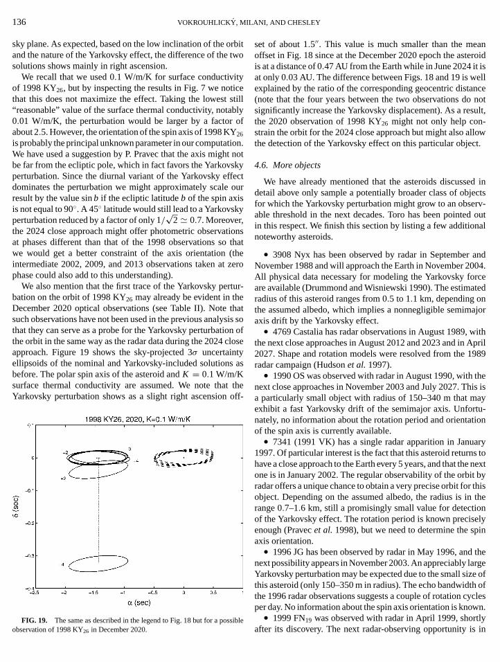
L

t

cs

i

e

y

i

te

s

nroidsellncenotult,

lowt.

d incts

rv-out

al

and04.ceted

ajor

ithpril989

theis isay-

ion

arys tonextbythisthe

nlyin

thergee ofofclesn.

ly


sky plane. As expected, based on the low inclination of the oand the nature of the Yarkovsky effect, the difference of thesolutions shows mainly in right ascension.

We recall that we used 0.1 W/m/K for surface conductivityof 1998 KY26, but by inspecting the results in Fig. 7 we notithat this does not maximize the effect. Taking the lowest“reasonable” value of the surface thermal conductivity, nota0.01 W/m/K, the perturbation would be larger by a factorabout 2.5. However, the orientation of the spin axis of 1998 KY26

is probably the principal unknown parameter in our computatWe have used a suggestion by P. Pravec that the axis mighbe far from the ecliptic pole, which in fact favors the Yarkovsperturbation. Since the diurnal variant of the Yarkovsky effdominates the perturbation we might approximately scaleresult by the value sinb if the ecliptic latitudeb of the spin axisis not equal to 90◦. A 45◦ latitude would still lead to a Yarkovskperturbation reduced by a factor of only 1/

√2' 0.7. Moreover,

the 2024 close approach might offer photometric observatat phases different than that of the 1998 observations sowe would get a better constraint of the axis orientation (intermediate 2002, 2009, and 2013 observations taken atphase could also add to this understanding).

We also mention that the first trace of the Yarkovsky perbation on the orbit of 1998 KY26 may already be evident in thDecember 2020 optical observations (see Table II). Notesuch observations have not been used in the previous analythat they can serve as a probe for the Yarkovsky perturbatiothe orbit in the same way as the radar data during the 2024 capproach. Figure 19 shows the sky-projected 3σ uncertaintyellipsoids of the nominal and Yarkovsky-included solutionsbefore. The polar spin axis of the asteroid andK = 0.1 W/m/Ksurface thermal conductivity are assumed. We note thatYarkovsky perturbation shows as a slight right ascension

FIG. 19. The same as described in the legend to Fig. 18 but for a possobservation of 1998 KY26 in December 2020.

ANI, AND CHESLEY

rbitwo

etillblyof

on.t notkyct

our

onsthat

thezero

ur-

thatis so

n oflose

as

theoff-

set of about 1.5′′. This value is much smaller than the meaoffset in Fig. 18 since at the December 2020 epoch the asteis at a distance of 0.47 AU from the Earth while in June 2024 it iat only 0.03 AU. The difference between Figs. 18 and 19 is wexplained by the ratio of the corresponding geocentric dista(note that the four years between the two observations dosignificantly increase the Yarkovsky displacement). As a resthe 2020 observation of 1998 KY26 might not only help con-strain the orbit for the 2024 close approach but might also althe detection of the Yarkovsky effect on this particular objec

4.6. More objects

We have already mentioned that the asteroids discussedetail above only sample a potentially broader class of objefor which the Yarkovsky perturbation might grow to an obseable threshold in the next decades. Toro has been pointedin this respect. We finish this section by listing a few additionnoteworthy asteroids.

• 3908 Nyx has been observed by radar in SeptemberNovember 1988 and will approach the Earth in November 20All physical data necessary for modeling the Yarkovsky forare available (Drummond and Wisniewski 1990). The estimaradius of this asteroid ranges from 0.5 to 1.1 km, depending onthe assumed albedo, which implies a nonnegligible semimaxis drift by the Yarkovsky effect.• 4769 Castalia has radar observations in August 1989, w

the next close approaches in August 2012 and 2023 and in A2027. Shape and rotation models were resolved from the 1radar campaign (Hudsonet al.1997).• 1990 OS was observed with radar in August 1990, with

next close approaches in November 2003 and July 2027. Tha particularly small object with radius of 150–340 m that mexhibit a fast Yarkovsky drift of the semimajor axis. Unfortunately, no information about the rotation period and orientatof the spin axis is currently available.• 7341 (1991 VK) has a single radar apparition in Janu

1997. Of particular interest is the fact that this asteroid returnhave a close approach to the Earth every 5 years, and that theone is in January 2002. The regular observability of the orbitradar offers a unique chance to obtain a very precise orbit forobject. Depending on the assumed albedo, the radius is inrange 0.7–1.6 km, still a promisingly small value for detectioof the Yarkovsky effect. The rotation period is known preciseenough (Pravecet al.1998), but we need to determine the spaxis orientation.• 1996 JG has been observed by radar in May 1996, and

next possibility appears in November 2003. An appreciably laYarkovsky perturbation may be expected due to the small sizthis asteroid (only 150–350 m in radius). The echo bandwidththe 1996 radar observations suggests a couple of rotation cyper day. No information about the spin axis orientation is know• 1999 FN19 was observed with radar in April 1999, short
ible
after its discovery. The next radar-observing opportunity is in

c.

i

yo

oh

,

o

s

-s in

in

pes

l

ehe

.with

d,r a

anddar-

mod-

ical

eling

ens,9.

er-

roid

tal

620

1620

r ob-


2018. Its small size, in the range 100–200 m, makes it an exlent candidate for revealing the Yarkovsky effect at that timeis worth noting that its recovery in 2018 would be improbabwithout the 1999 radar astrometry.

5. CONCLUSIONS

Although the problem of high orbital eccentricity has beesuccessfully dealt with in this paper, there remain a numberchallenging problems for future work. Most importantly, in acomputations of this paper we have applied a thermophysmodel based on a spherical body. For each of the asteroidsused a sphere with properly adjusted radius (so that the masthe asteroid is equal to the mass of its spherical approximatioHowever, the actual shape of these small objects is typicahighly irregular, and at the lowest level of approximation theshould be represented by a triaxial ellipsoid rather than bsphere. Developing the asteroid-tailored thermophysical mels for each of the cases would be valuable for refining resureported in this paper. Moreover, such models should take iaccount the complex evolution of the asteroid spin axis, in cotrast to the assumption of a constant orientation used throughthis work.

In light of the previous discussion we may say that alreain the next decade the orbit determination models of near-Eaasteroids will necessarily require that the Yarkovsky effectmodeled. However, we note that the conclusions of this pamay go even beyond this level. Acquiring radar observationdata for very small near-Earth asteroids, of which the obje1998 KY26 may be a first example, can leave us in a positiof studying the Yarkovsky effect in some detail. The size of torbital perturbation may allow us to not only detect the effeitself, but also to constrain some of the model parametersparticular the surface thermal conductivity. These parametmight, in turn, indicate the physical character of the objecsurface, thus complementing other types of observations.

ACKNOWLEDGMENTS

We thank G. Valsecchi for helpful discussions that initiated our workthis project and the other members of the OrbFit Consortium (M. Carpino aZ. Knezevic) for their contributions to the software system, that has been uin all the orbit determinations and observation predictions of this paper.are grateful to P. Chodas for assisting us with the correct interpretation ofradar data, and to S. Ostro for numerous suggestions that helped to shapfinal manuscript. We started this work with P. Farinella, whose suggestionscontributions were particularly valuable, but unfortunately he could not jous in the conclusive part of this research because of his health problemspremature death.

REFERENCES

Bottke, W. F., D. P. Rubincam, and J. A. Burns 2000. Dynamical evolutionmain belt meteoroids: Numerical simulations incorporating planetary pertbations and Yarkovsky thermal forces.Icarus145, 301–331.

Brouwer, D., and G. M. Clemence 1961.Methods of Celestial Mechanics. Aca-demic Press, New York.


el-It

le

nof

llcalwes ofn).llyyad-lts

nton-out

dyrth

beperalctne

ctin

erst’s

nnded

Wethee theandinand

ofur-

Broz, M., D. Vokrouhlicky, and P. Farinella 2000. Interaction of the Yarkovskydriven orbits of meteoroids and their precursors with the weak resonancethe main belt.Icarus, submitted for publication.

Casotto, S. 1992. Position and velocity perturbations in the orbital frameterms of classical element perturbations.Celest. Mech. Dynam. Astron.55,209–222.

De Angelis, G. 1995. Asteroid spin, pole and shape determinations.Planet.Space Sci.43, 649–682.

Drummond, J. D., and W. Z. Wisniewski 1990. The rotational poles and shaof 1580 Betulia and 3908 (1980PA) from one apparition.Icarus83, 349–359.

Farinella, P., and D. Vokrouhlický 1999. Semimajor axis mobility of asteroidafragments.Science283, 1507–1510.

Farinella, P., D. Vokrouhlický, and W. K. Hartmann 1998. Meteorite deliveryvia Yarkovsky orbital drift.Icarus132, 378–387.

Glegg, P. E., J. A. Bastin, and A. E. Gear 1966. Heat transfer in lunar rock.Mon.Not. R. Astron. Soc.133, 63–66.

Goldstein, R. M. 1969. Radar observations of Icarus.Science162, 903–904.

Graf, T., and K. Marti 1995. Collisional history of H chondrites.J. Geophys.Res.100, 21–47.

Harris, A. W. 1998. A thermal model for near-Earth asteroids.Icarus131, 291–301.

Hartmann, W. K., P. Farinella, D. Vokrouhlický, S. J. Weidenschilling, A.Morbidelli, F. Marzari, D. R. Davis, and E. Ryan 1999. Reviewing thYarkovsky effect: New light on the delivery of stones and irons from tasteroid belt.Meterit. Space Sci.34, A161–A168.

Herzog, G. F., S. Vogt, A. Albrecht, S. Xue, D. Fink, J. Klein, R. Middleton, HWeber, and L. Schultz 1997. Complex exposure histories for meteorites“short” exposure ages.Meteor. Planet. Sci.32, 413–422.

Hicks, M. D., M. S. Hanner, D. L. Rabinowitz, B. J. Burrati, T. J. HaywarU. Fink, and W. Grundy 1999. 6489 Golevka revisited: New evidence fopyroxene-rich near-Earth asteroid.Bull. Am. Astron. Soc.31, 1072.

Hudson, R. S., S. J, Ostro. and A. W. Harris 1997. Constraints on spin stateHapke parameters of Asteroid 4769 Castalia using lightcurves and a raderived shape model.Icarus130, 165–176.

Hudson, R. S., and 26 colleagues 2000. Radar observations and physicaleling of Asteroid 6489 Golevka.Icarus, in press.

Lieske, J. H., and G. W. Null 1969. Icarus and the determination of astronomconstants.Astron. J.74, 297–307.

Magnusson, P., and 46 colleagues 1997. Photometric observations and modof Asteroid 1620 Geographos.Icarus123, 227–244.

Mahapatra, P. R., S. J. Ostro, L. A. M. Benner, K. D. Rosema, R. F. JurgR. Winkler, R. Rose, J. D. Giorgini, D. K. Yeomans, and M. Slade 199Recent radar observations of Asteroid 1566 Icarus.Planet. Space Sci.47, 987–995.

Milani, A. 1999. The asteroid identification problem. I. Recovery of lost astoids.Icarus137, 269–292.

Mottola, S., and 28 colleagues 1997. Physical model of near-Earth aste6489 Golevka (1991 JX) from optical and infrared observations.Astron. J.114, 1234–1245.

Muller, T. G., J. S. V. Lagerros, and J. A. D. L. Blommaert 1999. Fundamenproperties and thermophysical modelling of asteroids after ISO.Bull. Am.Astron. Soc.31, 1075.

Ostro, S. J., and 11 colleagues 1995. Extreme elongation of Asteroid 1Geographos from radar images.Nature375, 474–476.

Ostro, S. J., and 12 colleagues 1996. Radar observations of AsteroidGeographos.Icarus121, 46–66.

Ostro, S. J., and 15 colleagues 1999a. Asteroids 4179 Toutatis: 1996 radaservations.Icarus137, 122–139.

Ostro, S. J., and 19 colleagues 1999b. Radar and optical observations of Asteroid1998 KY26.Science285, 557–559.

o

a

i

i

r

a-

as-

as-

the

avia.

maln

terial.

d I. I.

ites.


Pravec, P., M. Wolf, and L.Sarounov´a 1998. Lightcurves of 26 near-Earth asteroids.Icarus136, 124–153.

Rubincam, D. P. 1987. LAGEOS orbit decay due to infrared radiation frEarth.J. Geophys. Res.92, 1287–1294.

Rubincam, D. P. 1995. Asteroid orbit evolution due to thermal drag.J. Geophys.Res.100, 1585–1594.

Rubincam, D. P. 1998. Yarkovsky thermal drag on small asteroids and MEarth delivery.J. Geophys. Res.103, 1725–1732.

Shapiro, I. I., W. B. Smith, M. E. Ash, and S. Herrick 1971. General relativand the orbit of Icarus.Astron. J.76, 588–606.

Sitarski, G. 1992. On the relativistic motion of (1566) Icarus.Astron. J.104,1226–1229.

Sitarski, G. 1998. Motion of the minor planet 4179 Toutatis: Can we predictcollision with the Earth?Acta Astron.48, 547–561.

Spitale, J., and R. Greenberg 1999. Numerical investigation of the Yarkoveffect: Mutiny on the high e’s.Bull. Am. Astron. Soc.31, 1112.

Spitale, J., and R. Greenberg 2000. Numerical evaluation of the genYarkovsky effect: Effects on semimajor axis.Icarus, in press.

Veeder, G. J., M. S. Hanner, D. L. Matson, E. F. Tedesco, L. A. Lebofsand A. T. Tokunaga 1989. Radiometric of near-Earth asteroids.Astron. J.97,1211–1219.

Vokrouhlicky, D. 1998a. Diurnal Yarkovsky effect as a source of mobility ometer-sized asteroidal fragments: I. Linear theory.Astron. Astrophys.335,1093–1100.

Vokrouhlicky, D. 1998b. Diurnal Yarkovsky effect as a source of mobity of meter-sized asteroidal fragments: II. Non-sphericity Effects.Astron.Astrophys.338, 353–363.

Vokrouhlicky, D. 1999. A complete linear model for the Yarkovsky the
mal force on spherical asteroid fragments.Astron. Astrophys.344, 362–366.
ANI, AND CHESLEY

-

m

rs–

ty

its

sky

eral

ky,

f

l-

-

Vokrouhlicky, D., and M. Broz 1999. An improved model of the sesonal Yarkovsky force for the regolith-covered asteroid fragments.Astron.Astrophys.350, 1079–1084.

Vokrouhlicky, D., and P. Farinella 1998. The Yarkovsky seasonal effect onteroidal fragments: A nonlinearized theory for the plane-parallel case.Astron.J. 116, 2032–2041.

Vokrouhlicky, D., and P. Farinella 1999. The Yarkovsky seasonal effect onteroidal fragments: A non-linearized theory for spherical bodies.Astron. J.118, 3049–3060.

Vokrouhlicky, D., and P. Farinella 2000. Delivery of stony meteorites fromasteroid belt.Nature, in press.

Vokrouhlicky, D., M. Broz, P. Farinella, and Z. Kneˇzevic 2000. Yarkovsky-driven leakage of Koronis family members: I. The case of 2953 VysheslIcarus, in press.

Wechsler, A. E., P. E. Glaser, A. D. Little, and J. A. Fountain 1972. Therproperties of granulated materials. InThermal Characteristics of the Moo(J. W. Lucas, Ed.), pp. 215–241. MIT Press, Cambridge, MA.

Wesselink, A. J. 1948. Heat conductivity and nature of the lunar surface maBull. Astr. Inst. Nether.10, 351–363.

Yeomans, D. 1991. A comet among the near-Earth asteroids?Astron. J.101,1920–1928.

Yeomans, D. 1992. Erratum: “A comet among the near-Earth asteroids?”Astron.J. 104, 1266.

Yeomans, D., P. W. Chodas, M. S. Keesey, S. J. Ostro, J. F. Chandler, anShapiro 1992. Asteroid and comet orbits using radar data.Astron. J.103,303–317.

Yomogida, K., and T. Matsui 1983. Physical properties of ordinary chondrJ. Geophys. Res.88, 9513–9533.

Zaitsev, A. L., and 24 colleagues 1997. Intercontinental bistatic radar observa-tions of 6489 Golevka (1991 JX).Planet. Space Sci.45, 771–778.

yarkovsky effect on small near-earth asteroids

Documents