yuanyuan˜yang cong˜wang wireless rechargeable sensor …

123

S P R I N G E R B R I E F S I N E L E C T R I C A L A N D CO M P U T E R E N G I N E E R I N G

Yuanyuan YangCong Wang

Wireless Rechargeable Sensor Networks

SpringerBriefs in Electrical and ComputerEngineering

More information about this series at http://www.springer.com/series/10059

http://www.springer.com/series/10059

Yuanyuan Yang • Cong Wang

Wireless RechargeableSensor Networks

123

Yuanyuan YangDepartment of Electrical

and Computer EngineeringStony Brook UniversityStony Brook, NY, USA

Cong WangDepartment of Electrical

and Computer EngineeringStony Brook UniversityStony Brook, NY, USA

ISSN 2191-8112 ISSN 2191-8120 (electronic)SpringerBriefs in Electrical and Computer EngineeringISBN 978-3-319-17655-0 ISBN 978-3-319-17656-7 (eBook)DOI 10.1007/978-3-319-17656-7

Library of Congress Control Number: 2015936334

Springer Cham Heidelberg New York Dordrecht London© The Author(s) 2015This work is subject to copyright. All rights are reserved by the Publisher, whether the whole or part ofthe material is concerned, specifically the rights of translation, reprinting, reuse of illustrations, recitation,broadcasting, reproduction on microfilms or in any other physical way, and transmission or informationstorage and retrieval, electronic adaptation, computer software, or by similar or dissimilar methodologynow known or hereafter developed.The use of general descriptive names, registered names, trademarks, service marks, etc. in this publicationdoes not imply, even in the absence of a specific statement, that such names are exempt from the relevantprotective laws and regulations and therefore free for general use.The publisher, the authors and the editors are safe to assume that the advice and information in this bookare believed to be true and accurate at the date of publication. Neither the publisher nor the authors orthe editors give a warranty, express or implied, with respect to the material contained herein or for anyerrors or omissions that may have been made.

Printed on acid-free paper

Springer International Publishing AG Switzerland is part of Springer Science+Business Media (www.springer.com)

www.springer.com

www.springer.com

Recommended by Xuemin (Sherman) Shen

Preface

With an ever increasing demand of new wireless sensing applications, energyhas been the primary concern for wireless sensor networks. In particular, energyconservation has been studied extensively to extend network lifetime. A variety ofapproaches have been proposed in literature that can elongate network lifetime tosome extent. However, with limited energy storage, sensor’s battery would depleteeventually and replacing those batteries requires tremendous human efforts.

In this book, we describe a new approach to replenishing sensor’s battery viawireless charging without wires or plugs. We start with a detailed overview ofthe recent developments in wireless charging technologies and their applicationsin wireless sensor networks to highlight the advantages and disadvantages. We thenprovide a new hierarchical network architecture that adopts a mobile vehicle forwireless charging. We name such networks Wireless Rechargeable Sensor Networks(WRSNs). Based on this network architecture, we discuss several principles fromtheoretical aspects, and design communication protocols and recharge schedul-ing algorithms to maintain perpetual network operations. We also give networkperformance evaluation results in various criteria such as nonfunctional nodepercentage, network latency, and energy overhead. The state-of-the-art wirelesscharging technology covered in this book would help readers understand existingchallenges and inspire future research to improve energy efficiency and networklifetime for wireless sensor networks.

Stony Brook, NY, USA Yuanyuan YangFebruary 2015 Cong Wang

vii

Acknowledgments

The writing of this book was supported in part by the grant from US NationalScience Foundation under grant number ECCS-1307576.

ix

Contents

1 Introduction . . . . . . . . . . . . . . . . . . . . . . . . . . . . . . . . . . . . . . . . . . . . . . . . . . . . . . . . . . . . . . . . . . . 11.1 Introduction and Background . . . . . . . . . . . . . . . . . . . . . . . . . . . . . . . . . . . . . . . . . . 11.2 Wireless Charging Technology . . . . . . . . . . . . . . . . . . . . . . . . . . . . . . . . . . . . . . . . 3

1.2.1 Electromagnetic Radiation . . . . . . . . . . . . . . . . . . . . . . . . . . . . . . . . . . . . . 31.2.2 Magnetic Resonant Coupling . . . . . . . . . . . . . . . . . . . . . . . . . . . . . . . . . . 4

1.3 Summary . . . . . . . . . . . . . . . . . . . . . . . . . . . . . . . . . . . . . . . . . . . . . . . . . . . . . . . . . . . . . . . . 5References . . . . . . . . . . . . . . . . . . . . . . . . . . . . . . . . . . . . . . . . . . . . . . . . . . . . . . . . . . . . . . . . . . . . . . 5

2 Network Architecture and Principles . . . . . . . . . . . . . . . . . . . . . . . . . . . . . . . . . . . . . . . 92.1 Network Components . . . . . . . . . . . . . . . . . . . . . . . . . . . . . . . . . . . . . . . . . . . . . . . . . . 92.2 Principles in Wireless Rechargeable Sensor Networks . . . . . . . . . . . . . . . 11

2.2.1 Energy Neutrality. . . . . . . . . . . . . . . . . . . . . . . . . . . . . . . . . . . . . . . . . . . . . . . 112.2.2 Estimation of Node Lifetime. . . . . . . . . . . . . . . . . . . . . . . . . . . . . . . . . . . 132.2.3 Adaptive Recharge Threshold . . . . . . . . . . . . . . . . . . . . . . . . . . . . . . . . . 14


3 Distributed Node Status Reporting Protocol . . . . . . . . . . . . . . . . . . . . . . . . . . . . . . . 173.1 Overview . . . . . . . . . . . . . . . . . . . . . . . . . . . . . . . . . . . . . . . . . . . . . . . . . . . . . . . . . . . . . . . . 173.2 Protocol Design . . . . . . . . . . . . . . . . . . . . . . . . . . . . . . . . . . . . . . . . . . . . . . . . . . . . . . . . . 18

3.2.1 Head Election . . . . . . . . . . . . . . . . . . . . . . . . . . . . . . . . . . . . . . . . . . . . . . . . . . . 183.2.2 Status Request . . . . . . . . . . . . . . . . . . . . . . . . . . . . . . . . . . . . . . . . . . . . . . . . . . 193.2.3 Status Report and Recharge. . . . . . . . . . . . . . . . . . . . . . . . . . . . . . . . . . . . 203.2.4 Emergency Report and Recharge . . . . . . . . . . . . . . . . . . . . . . . . . . . . . . 213.2.5 Head Hierarchy Maintenance . . . . . . . . . . . . . . . . . . . . . . . . . . . . . . . . . . 22


xi

xii Contents

4 Recharge Scheduling . . . . . . . . . . . . . . . . . . . . . . . . . . . . . . . . . . . . . . . . . . . . . . . . . . . . . . . . . 254.1 Emergency Recharge Scheduling Problem . . . . . . . . . . . . . . . . . . . . . . . . . . . . 254.2 Normal Recharge Scheduling . . . . . . . . . . . . . . . . . . . . . . . . . . . . . . . . . . . . . . . . . . 28

4.2.1 Weighted-Sum Algorithm. . . . . . . . . . . . . . . . . . . . . . . . . . . . . . . . . . . . . . 314.2.2 Adaptive Recharge Scheduling Algorithm . . . . . . . . . . . . . . . . . . . . 32


5 Performance Evaluations . . . . . . . . . . . . . . . . . . . . . . . . . . . . . . . . . . . . . . . . . . . . . . . . . . . . 435.1 Parameter Settings . . . . . . . . . . . . . . . . . . . . . . . . . . . . . . . . . . . . . . . . . . . . . . . . . . . . . . 435.2 Comparison of Recharge Scheduling Algorithms. . . . . . . . . . . . . . . . . . . . . 445.3 Node Nonfunctionality . . . . . . . . . . . . . . . . . . . . . . . . . . . . . . . . . . . . . . . . . . . . . . . . . 445.4 Energy Evolution . . . . . . . . . . . . . . . . . . . . . . . . . . . . . . . . . . . . . . . . . . . . . . . . . . . . . . . 455.5 Duration of Nonfunctional Status . . . . . . . . . . . . . . . . . . . . . . . . . . . . . . . . . . . . . . 475.6 Data Collection Latency . . . . . . . . . . . . . . . . . . . . . . . . . . . . . . . . . . . . . . . . . . . . . . . . 485.7 Overhead of Node Status Collection Protocol. . . . . . . . . . . . . . . . . . . . . . . . . 495.8 Charging Vehicle’s Moving Energy Cost . . . . . . . . . . . . . . . . . . . . . . . . . . . . . . 495.9 Comparison with Static Optimization Approach . . . . . . . . . . . . . . . . . . . . . . 515.10 Summary . . . . . . . . . . . . . . . . . . . . . . . . . . . . . . . . . . . . . . . . . . . . . . . . . . . . . . . . . . . . . . . . 52References . . . . . . . . . . . . . . . . . . . . . . . . . . . . . . . . . . . . . . . . . . . . . . . . . . . . . . . . . . . . . . . . . . . . . . 52

6 Conclusions . . . . . . . . . . . . . . . . . . . . . . . . . . . . . . . . . . . . . . . . . . . . . . . . . . . . . . . . . . . . . . . . . . . . 53

Glossary . . . . . . . . . . . . . . . . . . . . . . . . . . . . . . . . . . . . . . . . . . . . . . . . . . . . . . . . . . . . . . . . . . . . . . . . . . . . 55

Acronyms

AC Alternating CurrentDC Direct CurrentCMST Capacitated Minimum Spanning TreeCVRP Capacitated Vehicle Routing ProblemEIRP Effective Isotropic Radiated PowerEV Electrical VehicleEW Esau-WilliamsFCC Federal Communication CommissionTSP Traveling Salesman ProblemVRP Vehicle Routing ProblemVRPTW Vehicle Routing Problem with Time WindowsWRSN Wireless Rechargeable Sensor NetworkWSN Wireless Sensor Network

xiii

Chapter 1Introduction

1.1 Introduction and Background

The next generation wireless networks rely on sensors to identify and extract usefulinformation from the environment. With the option to mount various types ofdetectors ranging from temperature, magnetic, pressure, acoustic sensors to morecomplex gyroscope, imaging, infrared, video sensors, wireless sensor networks(WSNs) provide an easy way to access information in the physical world [1, 2].It begins to find an increasing number of applications from our daily life to manymission-critical tasks. Typical examples in our daily life include temperature andhumidity sensors deployed indoors that can automatically control the climate. Inmission-critical tasks such as volcano or forest fire monitoring [3, 4], sensors alsoplay an irreplaceable role to provide accurate readings on time. For example,the traditional forest fire monitoring system depends on the analysis of satelliteimages. However, the accuracy of these systems is usually limited by image qualityand weather conditions. Sensors equipped with thermal imaging and temperaturedetectors can be deployed and transmit real-time data in a designated area [4].

The increasing demand for more complex sensors leads to higher energyconsumption on sensor nodes. To this end, energy conservation has been oneof the primary focuses in WSN research in the past decade. Since replacingsensor’s battery is infeasible or risky in many applications [3, 4], most of theresearch aims to maximize network lifetime. For a single node, duty cycling isone of the most effective methods to save energy [10]. It puts radio transceiversin sleep mode whenever there is no communication. To adopt this method in anetwork, wakeup/sleep scheduling of sensors is required to guarantee end-to-endcommunications [11, 12]. In addition, battery-aware routing and scheduling basedon battery recovery property have been studied to extend sensor node lifetime[13–15]. At the network level, researchers have considered maximizing networklifetime by optimizing either flow routing [16] or sensor missions [17, 18]. Besides,how data is collected also determines network lifetime. Traditional approach to

© The Author(s) 2015Y. Yang, C. Wang, Wireless Rechargeable Sensor Networks, SpringerBriefsin Electrical and Computer Engineering, DOI 10.1007/978-3-319-17656-7_1

1

2 1 Introduction

aggregating sensed data through a static data sink is known to be less energy efficientsince nodes close to the sink consume more energy to relay packets. These nodesusually form a bottleneck around the sink and put an upper limit on the networklifetime while other nodes may still have energy. This is regarded as the infamous“energy hole problem” [19]. A solution is to introduce a mobile data sink for datagathering [20–26]. It has been shown [25] that by carefully planning trajectory ofthe mobile sink, energy consumptions on sensor nodes can be balanced and networklifetime can be extended significantly.

Although these methods can prolong network lifetime to some extent, sensor’sbattery would deplete eventually and cause service interruptions. A promisingtechnique is to renew sensor’s battery by harvesting environmental energy such assolar and wind [5–7]. For example, solar harvesting can provide energy from solarpanels of similar size to sensor nodes [8]. It is also shown that multiple ambientenergy sources can be utilized to power sensor nodes in [9]. However, an inevitabledrawback of environmental energy harvesting is due to the inherent dynamics ofenergy sources. When energy sources are not available, sensor nodes may stopworking and it can lead to long data latency or data loss in the network.

Recently, finding an easy and reliable way to replenish sensor’s battery beginsto attract more attentions in the sensor network research community. Fortunately,breakthroughs in wireless charging technology have opened up a new dimension topower sensor nodes in distance without any wires or plugs. Pioneered by NikolaTesla [27] a century ago, it is only recently wireless charging enjoys so muchpopularity after the experimental realization by Kurs et al. [28]. It has been shownin [28] that a total of 60 W energy can be transferred between two magneticallycoupled coils over an air gap of 2 m with 40 % efficiency. The experimentalprototype is soon extended to power multiple devices in [29]. In the meanwhile, fastdevelopment of mobile devices and stagnant battery technology deliver the impetusto drive wireless charging technology into commercialization and many productsare now available. For example, charging pad called “Powermat c�” can rechargemultiple cell phones and PDAs simultaneously by simply putting them on thepad [30]. Powercast c� systems realize wireless charging for sensing devices up toseveral meters away [31]. This technology has demonstrated not only the strengthsto power small portable devices, but also the potentials to recharge ElectricalVehicles (EVs). With the ability to deliver 100 W of energy at high efficiency,wireless charging systems can be launched at power stations, parking lots or evenbeneath road surface to recharge EVs without any physical contact [32].

The main focus of this book is to examine how to employ wireless chargingin traditional battery-powered wireless sensor networks and we call such networksWireless Rechargeable Sensor Networks (WRSNs) henceforth. We start with adetailed overview of the recent developments in wireless charging technologies andtheir applications in WSNs to highlight the advantages and disadvantages. We thenintroduce controlled mobility to a hierarchical network in order to provide efficiencyand scalability. Based on the new network architecture, we discuss several importantprinciples from theoretical aspects. We also provide a distributed communicationprotocol for gathering node status information in real-time, followed by recharge

1.2 Wireless Charging Technology 3

scheduling algorithms that aim to maintain perpetual network operations. Finally,we give network performance evaluation results in various criteria such as nonfunc-tional node percentage, network latency, energy overhead, etc.

1.2 Wireless Charging Technology

In this section, we introduce two major techniques of wireless charging: electromag-netic radiation and magnetic resonant coupling, and their applications in WSNs.

1.2.1 Electromagnetic Radiation

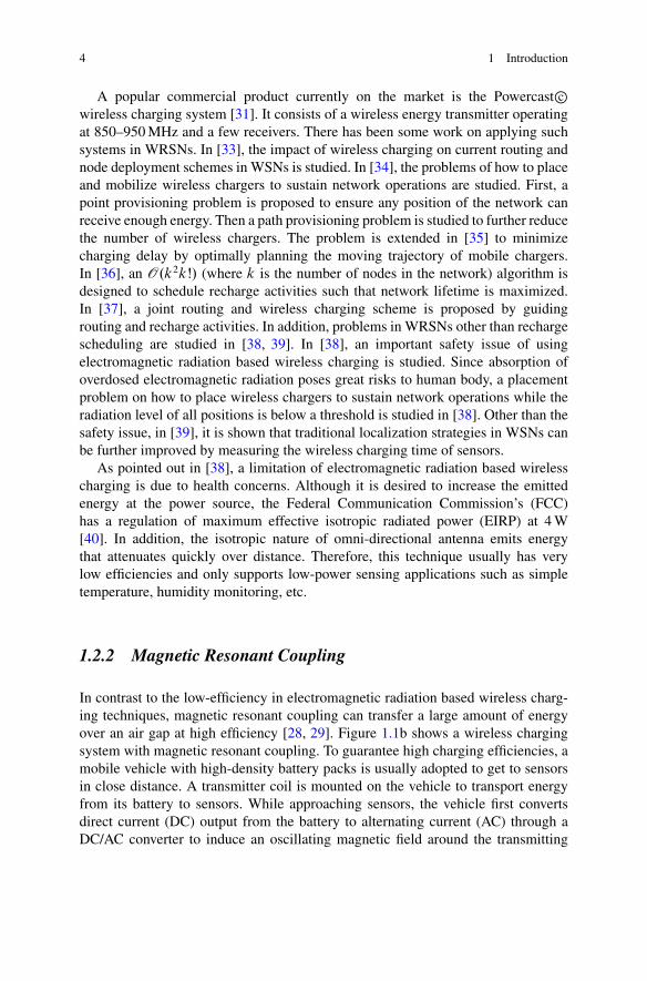
Electromagnetic waves have been used for communications since the last century.Recently, upon discovering the energy resides in the electromagnetic waves canbe captured to power ultra-low power devices, a great amount of research effortshave been devoted to scavenge energy in the ubiquitous electromagnetic waves.There are plenty of such energy sources such as TV towers, cellular stations or evenlocal Wi-Fi access points. However, due to the nature of isotropic wave propagation,received signal strength decreases dramatically with transmission distance. Thusonly a very small fraction of energy can be effectively captured from the air.Figure 1.1a shows a sketch of an electromagnetic radiation based wireless chargingsystem.

Transmit AntennaReceive Antenna

voltage

input load

a

b

Transmitter Circuit Receiver Circuit

Coupling

Fig. 1.1 Wireless charging systems. (a) Electromagnetic radiation. (b) Magnetic resonantcoupling

4 1 Introduction

A popular commercial product currently on the market is the Powercast c�wireless charging system [31]. It consists of a wireless energy transmitter operatingat 850–950 MHz and a few receivers. There has been some work on applying suchsystems in WRSNs. In [33], the impact of wireless charging on current routing andnode deployment schemes in WSNs is studied. In [34], the problems of how to placeand mobilize wireless chargers to sustain network operations are studied. First, apoint provisioning problem is proposed to ensure any position of the network canreceive enough energy. Then a path provisioning problem is studied to further reducethe number of wireless chargers. The problem is extended in [35] to minimizecharging delay by optimally planning the moving trajectory of mobile chargers.In [36], an O.k2kŠ/ (where k is the number of nodes in the network) algorithm isdesigned to schedule recharge activities such that network lifetime is maximized.In [37], a joint routing and wireless charging scheme is proposed by guidingrouting and recharge activities. In addition, problems in WRSNs other than rechargescheduling are studied in [38, 39]. In [38], an important safety issue of usingelectromagnetic radiation based wireless charging is studied. Since absorption ofoverdosed electromagnetic radiation poses great risks to human body, a placementproblem on how to place wireless chargers to sustain network operations while theradiation level of all positions is below a threshold is studied in [38]. Other than thesafety issue, in [39], it is shown that traditional localization strategies in WSNs canbe further improved by measuring the wireless charging time of sensors.

As pointed out in [38], a limitation of electromagnetic radiation based wirelesscharging is due to health concerns. Although it is desired to increase the emittedenergy at the power source, the Federal Communication Commission’s (FCC)has a regulation of maximum effective isotropic radiated power (EIRP) at 4 W[40]. In addition, the isotropic nature of omni-directional antenna emits energythat attenuates quickly over distance. Therefore, this technique usually has verylow efficiencies and only supports low-power sensing applications such as simpletemperature, humidity monitoring, etc.

1.2.2 Magnetic Resonant Coupling

In contrast to the low-efficiency in electromagnetic radiation based wireless charg-ing techniques, magnetic resonant coupling can transfer a large amount of energyover an air gap at high efficiency [28, 29]. Figure 1.1b shows a wireless chargingsystem with magnetic resonant coupling. To guarantee high charging efficiencies, amobile vehicle with high-density battery packs is usually adopted to get to sensorsin close distance. A transmitter coil is mounted on the vehicle to transport energyfrom its battery to sensors. While approaching sensors, the vehicle first convertsdirect current (DC) output from the battery to alternating current (AC) through aDC/AC converter to induce an oscillating magnetic field around the transmitting

References 5

coil. On the sensor side, the receiving coil is tuned to resonate at the same frequency.An alternating current is generated at the sensor’s output circuit. The AC is thenconverted back to DC to recharge sensor’s battery.

The potentials of using magnetic resonant coupling in WRSNs is studied in[41–45]. In [42], an optimization problem to maximize the ratio between chargingvehicle idling and working time is studied. A Hamiltonian cycle through all thesensor nodes is proved to be the shortest recharge path. Instead of rechargingall the nodes, in [41], only a number of nodes request for recharge are serviced,and this number is upper bounded by a tour length threshold to guarantee datalatency. During recharge, the charging vehicle simultaneously gathers data fromthe neighborhood in multi-hops and uploads all collected data to the base stationafter a recharging cycle is completed. A system-wide optimization is performedto maximize network utility by selecting optimal data rates and flow routing. In[44], optimal allocation of vehicle’s stopping time to recharge sensors at differentlocations is studied. Upon realizing the dynamics in sensors’ energy consumptions,to provide more accurate recharge decisions, a recharge framework is proposed in[45]. An NP-hard problem to minimize the movement cost of charging vehicles isstudied and several heuristic algorithms are proposed. In sum, magnetic resonantcoupling is a promising technology ready to support many energy-demandingmultimedia applications with enormous data communication and sensing activities.Therefore, in this book, we focus on applying this technology in WSNs.

1.3 Summary

In this chapter, we have presented a brief introduction to wireless chargingtechnology and its application in WSNs. We discuss its latest advances and describetwo typical techniques to perform wireless charging followed by a literature reviewof the most recent works in wireless sensor research community. The subsequentchapters provide a detailed coverage of several important issues in WRSNs includ-ing the basic network architecture, components, principles, a distributed node statusreporting protocol, recharge scheduling algorithms and performance evaluations.

References

1. I. Akyildiz, “Wireless sensor networks: a survey,” Computer networks, vol. 38, no. 4,pp. 393–422, 2002.

2. K. Sohrabi, “Protocols for self-organization of a wireless sensor network,” IEEE personalcommunications, vol. 7, no. 5, pp. 16–27, 2000.

3. W. A. Geoffrey, “Deploying a wireless sensor network on an active volcano,” IEEE InternetComputing, vol. 10, no. 2, pp. 18–25, 2006.

4. L. Yu, N. Wang, X. Meng, “Real-time forest fire detection with wireless sensor networks,”IEEE International Conference on Wireless Communications, Networking and Mobile Com-puting, vol.2, pp.1214–1217, 2005.

6 1 Introduction

5. T. Voigt, H. Ritter, J. Schiller ,“Utilizing solar power in wireless sensor networks,” IEEEInternational Conference on Local Computer Networks (LCN), 2003.

6. M. Rahimi, H. Shah, G. Sukhatme, J. Heideman and D. Estrin, “Studying the feasibility ofenergy harvesting in a mobile sensor network,” IEEE International Conference on Roboticsand Automation, 2003.

7. C. Wang, S. Guo and Y. Yang, “Energy-efficient mobile data collection in energy-harvestingwireless sensor networks,” The 20th IEEE International Conference on Parallel and Dis-tributed Systems (ICPADS 2014), Hsinchu, Taiwan, Dec. 2014.

8. J. Paradiso, T. Starner, “Energy scanverging for mobile and wireless electronics,” IEEE Journalof Pervasive Computing, vol. 4, no. 1, pp. 18–27, 2005.

9. C. Park and P. H. Chou, “AmbiMax: autonomous energy harvesting platform for multi-supplywireless sensor nodes,” IEEE International Conference on Sensing, Communication, andNetworking (SECON), vol. 1, pp. 168–177, 2006.

10. W. Ye, J. Heidemann, D. Estrin, “An energy-efficient MAC protocol for wireless sensornetworks,” IEEE INFOCOM, vol.3, pp. 1567–1576, 2002.

11. A. Keshavarzian, H. Lee and L. Venkatraman, “Wakeup scheduling in wireless sensornetworks,” ACM International Symposium on Mobile Ad Hoc Networking and Computing(MobiHoc), pp. 322–333, 2006.

12. Z. Zhang, M. Ma and Y. Yang, “Energy-efficient multi-hop polling in clusters of two-layeredheterogeneous sensor networks,” IEEE Transactions on Computers, vol. 57, no. 2, pp. 231–245,Feb. 2008.

13. C. Ma and Y. Yang, “A battery-aware scheme for routing in wireless ad hoc networks,” IEEETransactions on Vehicular Technology, vol. 60, no. 8, pp. 3919–3932, Oct. 2011.

14. C. Ma, Z. Zhang and Y. Yang, “Battery-aware scheduling in wireless mesh networks,”ACM/Springer Mobile Networks & Applications (MONET), vol. 13, pp. 228–241, 2008.

15. C. Ma and Y. Yang, “Battery-aware routing for streaming data transmissions in wirelesssensor networks,” ACM/Springer Mobile Networks & Applications (MONET), vol. 11, no. 5,pp. 757–767, October 2006.

16. C. J. Hwan and L. Tassiulas, “Maximum lifetime routing in wireless sensor networks.”IEEE/ACM Transactions on Networking, vol. 12, no. 4, pp. 609–619, 2004.

17. M. Bhardwaj and A.P. Chandrakasan, “Bounding the lifetime of sensor networks via optimalrole assignments,” IEEE INFOCOM, 2002.

18. M. Cardei, M. T. Thai, Y. Li, W. Wu, “Energy-efficient target coverage in wireless sensornetworks,” IEEE INFOCOM, 2005.

19. X. Wu, G. Chen and S. Das, “Avoiding energy holes in wireless sensor networks withnonuniform node distribution,” IEEE Transactions on Parallel and Distributed Systems, vol.19,no.5, pp. 710–720, 2008.

20. M. Ma and Y. Yang, “SenCar: An energy efficient data gathering mechanism for large scalemultihop sensor networks,” IEEE Transactions on Parallel and Distributed Systems, vol. 18,no. 10, pp. 1476–1488, October 2007.

21. J. Luo, J. P. Hubaux, “Joint sink mobility and routing to maximize the lifetime of wirelesssensor networks: the case of constrained mobility,” IEEE/ACM Transactions on Networking,vol. 18, no. 3, pp. 871–884, June 2010.

22. M. Zhao and Y. Yang, “Bounded relay hop mobile data gathering in wireless sensor networks,”IEEE Transactions on Computers, vol. 61, no. 2, pp. 265–277, Feb. 2012.

23. M. Zhao. M. Ma and Y. Yang, “Efficient data gathering with mobile collectors and space-division multiple access technique in wireless sensor networks,” IEEE Transactions onComputers, vol. 60, no. 3, pp. 400–417, March 2011.

24. M. Zhao and Y. Yang, “Optimization based distributed algorithms for mobile data gathering inwireless sensor networks,” IEEE Transactions on Mobile Computing, vol. 11, no. 10, pp. 1464–1477, October 2012.

25. M. Ma, Y. Yang and M. Zhao, “Tour planning for mobile data gathering mechanisms in wirelesssensor networks,” IEEE Transactions on Vehicular Technology, vol. 62, no. 4, pp. 1472–1483,May 2013.

References 7

26. M. Zhao, Y. Yang and C. Wang, “Mobile data gathering with load balanced clustering anddual data uploading in wireless sensor networks” to appear in IEEE Transactions on MobileComputing, 2015.

27. N. Tesla, “Apparatus for transmitting electrical energy,” U.S. Patent 11119732, Dec. 1914.28. A. Kurs, A. Karalis, R. Moffatt, J. D. Joannopoulos, P. Fisher and M. Soljacic, “Wireless power

transfer via strongly coupled magnetic resonances,” Science, vol. 317, pp. 83, 2007.29. A. Kurs, R. Moffatt and M. Soljacic, “Simultaneous mid-range power transfer to multiple

devices,”Applied Physics Letter, vol. 96, no. 4, article 4102, Jan. 2010.30. Powermat c�, “http://www.powermat.com.”31. Powercast Corp c�, “http://www.powercastco.com”.32. Hevo power c�, “http://www.hevopower.com.”33. B. Tong, Z. Li, G. Wang and W. Zhang, “How wireless power charging technology affects

sensor network deployment and routing,” IEEE Distributed Computing Systems (ICDCS),2010.

34. S. He, J. Chen, F. Jiang, D. Yau, G. Xing and Y. Sun,“Energy provisioning in wirelessrechargeable sensor networks,” IEEE Transactions on Mobile Computing, vol. 12, no. 10,pp. 1931–1942, Oct. 2013.

35. L. Fu, P. Cheng, Y. Gu, J. Chen and T. He, “Minimizing charging delay in wireless rechargeablesensor networks,” IEEE INFOCOM, pp. 2922–2930, 2013.

36. Y. Peng, Z. Li, W. Zhang and D. Qiao, “Prolonging sensor network lifetime through wirelesscharging,” IEEE Real-Time Systems Symposium (RTSS), pp. 129–139, 2010.

37. Z. Li, P. Yang, W. Zhang, and D. Qiao, “J-RoC: a Joint Routing and Charging Scheme toProlong Sensor Network Lifetime”, IEEE International Conference on Network Protocols(ICNP), 2011.

38. H. Dai, Y. Liu, G. Chen, X. Wu and T. He,“Safe charging for wireless power transfer,” IEEEINFOCOM, pp. 1105–1113, 2014.

39. Y. Shu, P. Cheng, Y. Gu, J. Chen and T. He,“TOC: Localizing wireless rechargeable sensorswith time of charge,” IEEE INFOCOM, pp. 388–396, 2014.

40. Online: “http://www.afar.net/tutorials/fcc-rules”.41. M. Zhao, J. Li and Y. Yang, “Joint mobile energy replenishment and data gathering in wireless

rechargeable sensor networks,” IEEE Transactions on Mobile Computing, vol. 13, no. 12,pp. 2689–2705, 2014.

42. Y. Shi, L. Xie, T. Hou and H. Sherali, “On renewable sensor networks with wireless energytransfer,” IEEE INFOCOM, pp. 1350–1358, 2011.

43. L. Xie, Y. Shi, T. Hou, W. Lou, H. Sherali and S. Midkiff, “On the renewable sensor networkswith wireless energy transfer: the multi-node case,” IEEE International Conference on Sensing,Communication, and Networking (SECON), 2012.

44. S. Guo, C. Wang and Y. Yang, “Joint mobile data gathering and energy provisioning in wirelessrechargeable sensor networks,” IEEE Transactions on Mobile Computing, vol. 13, no. 12,pp. 2836–2852, 2014.

45. C. Wang, J. Li, F. Ye and Y. Yang, “NETWRAP: An NDN based real-time wireless rechargingframework for wireless sensor networks,” IEEE Transactions on Mobile Computing, vol. 13,no. 6, pp. 1283–1297, 2014.

http://www.powermat.com

http://www.powercastco.com

http://www.hevopower.com

http://www.afar.net/tutorials/fcc-rules

Chapter 2Network Architecture and Principles

2.1 Network Components

Assume that sensor nodes are uniformly and randomly distributed in the network,and nodes are stationary and each node knows its deployed location. For scalableperformance, the network is divided into several areas and each area is furtherdivided to generate some new sub-areas. A new level is generated in each division.The divisions are based on geographical coordinates of the sensing field. Anexample of a 2-level WRSN network is shown in Fig. 2.1. The two areas representedby solid lines are generated at the first level. Then each area is further split intotwo sub-areas represented by dashed lines on the second level. Several key networkcomponents are explained below.

• Charging Vehicles: A charging vehicle has positioning systems (GPS) and knowsits location. The sensor locations are pre-processed during network initializationand known to the charging vehicles. The vehicles are equipped with high densitybattery packs and charging coils. They also have communication capability bylaunching powerful antennas. In this way, they can not only query the networkfor node status information but also communicate among themselves or to thebase station via long range communication technologies (e.g., cellular, WiMax).

• Base Station: The base station is used for collecting sensing data and performingnetwork management. The charging vehicles can be commanded remotely bythe network administrator via the base station. It also has computing capabilitiesto perform the tasks of calculating recharge sequences and dispatching chargingvehicles. When a charging vehicle almost depletes its own energy, it returns tothe base station for a quick battery replacement.

• Head Nodes: A head node is a sensor node that aggregates node’s statusinformation in its subordinate area. When requested by a charging vehicle orthe head node of its superior level, it aggregates node status information from thesubordinate sub-areas at the lower levels and sends to the requester.


9

10 2 Network Architecture and Principles

Fig. 2.1 Network architecture

• Proxy Nodes: An emergency occurs when a node’s battery energy falls belowa threshold (e.g., 10 %). It needs to be handled by the charging vehiclesimmediately. The head nodes on the top-level are selected as proxies so theycan aggregate emergency information from sensor nodes directly without propa-gating through the network hierarchy.

• Normal Nodes: A sensor node not selected as a head is a normal node. It reportsits status information to its superior head node, or sends emergency informationdirectly to its proxy when the battery energy drops below the recharge threshold.

Let N denote the total number of sensor nodes in the network and L denotethe side length of the square sensing field. Then the node density is � D N

L2 .For event-driven sensing applications with events occurring at each location withequal probability, spatially and temporally independent of each other, the datageneration process can be modeled as a Poisson process with average rate � [1].All sensors transmit at the same power level with fixed transmission range r . Theenergy consumed for transmitting/receiving a packet is et and er , respectively. Toobtain their values with respect to packet length l , we can utilize the model in [2].The base station is placed at the center of the field to collect sensed data in multi-hops. When receiving a status request, a sensor node transmits its status informationincluding energy level and lifetime to the head node in the sub-area. If its energydrops below the emergency threshold, it sends out an emergency recharge requestto the proxy node.

The network has m charging vehicles. Once the recharging voltage at the sensor’soutput circuit is enough to provide a charge, the recharge time is governed by batterycharacteristics. The typical recharge time required to bring battery energy from zeroto full capacity Cs is Tr time (e.g., for a Panasonic Ni-MH AAA battery [3] ofbattery capacity Cs D 780 mAh, Tr D 78 min). All charging vehicles are equippedwith high-density batteries of Ch.Ch � Cs/ and consume at ec J=m while movingat speed v m=s.

2.2 Principles in Wireless Rechargeable Sensor Networks 11

2.2 Principles in Wireless Rechargeable Sensor Networks

In this section, we introduce several principles in WRSNs from the theoreticalaspects. These include energy neutrality, number of charging vehicles, node lifetimeand adaptive recharge threshold.

2.2.1 Energy Neutrality

For a WRSN, the principle of energy neutrality must hold. That is,

E.T / � R.T / C E0 (2.1)

where T is the time duration, E.T / is the total energy consumption of the networkin T , R.T / is the total energy replenished into the network by the charging vehiclesin T and E0 is the initial energy of all the nodes. In other words, the energy neutralcondition states that the energy consumption of all the sensor nodes must be lessthan or equal to the total energy available in a long time perspective. Otherwise,nodes in the network would deplete energy eventually.

We can obtain the number of charging vehicles needed to satisfy Eq. (2.1). First,let us estimate R.T /. Since recharge time depends on the specific battery charac-teristics, the maximum energy a charging vehicle can put back into the network inTr time is at most Cs . The maximum charging capacity occurs when the vehiclerecharges nodes one after another without any idling time in between. The averagemoving time between two consecutive sensor locations can be estimated throughthe average distance between two random locations in the square field of length

L. From [5], we obtain the average distance d D 2p

2C10 ln.p

2C1/C4

30L � 0:52L.

For charging vehicles moving at constant speed v m/minute, the amount of energyreplenished into the network is,

R.T / D mCsT

0:52L=v C Tr

: (2.2)

E.T / on the left hand side of Eq. (2.1) is a random variable since the packet

generation process is Poisson. The network with length L has at most h D dp

2L2r

ehops to the boundaries. As studied in [4], it can be closely approximated by h

concentric rings and each inner ring carries traffic from all outer rings. Since nodesare uniformly and randomly distributed, the number of nodes in the i -th corona,is Ni D .2i � 1/r2�� for 0 < i � h. We start with the estimation of energy


consumption in each ring. The average energy consumption for the i -th ring is(0 < i � h),

�i D Ni �Tet ChX

jDiC1

Nj �T .et C er /

D r2��T�.h2 � i 2/.et C er / C .2i � 1/et

�(2.3)

By summing Eq. (2.3) from 1 to h, we obtain the total network energy consumption

E.T / D"

hX

iD1

.h2 � i 2/.et C er / C .2i � 1/er

#r2��T

D��

2

3h3 � 1

2h2 � 1

6h

�.et C er / C h2et

�r2��T (2.4)

Note that the derivation of total energy consumption is based on the fact that nodesgenerate packets independently and randomly following a Poisson process and thesum of Poisson random variables are still Poisson with mean equal to the sum oftheir average rates.

We can now plug R.T / and E.T / into Eq. (2.1). We have the following theorem.

Theorem 1. The probability for the energy neutral condition to hold is

Pop D ˚

0

[email protected] / C E0 � E.T /

qE.T /

1

CA (2.5)

where R.T / and E.T / are obtained in Eqs. (2.2) and (2.4), respectively. ˚.�/denotes the Cumulative Distribution Function of the Normal distribution.

Proof. Energy consumption in the network is taken by the sum of independentPoisson variables over T . When T is observed over a long time period, we canuse the Central Limit Theorem to approximate Poisson distribution by a Normaldistribution N .E.T /; E.T // (note that the mean and variance of a Poissondistribution is the same) [6].

From Theorem 1, we immediately have the following Proposition.

Proposition 1. The minimum number of charging vehicles required to maintainperpetual operation is

m D

2

6666

.˚�1.�/

qE.T / C E.T / � E0/.0:52L=v C Tr/

CsT

3

7777(2.6)

2.2 Principles in Wireless Rechargeable Sensor Networks 13

where ˚�1.�/ is the inverse Cumulative Distribution Function of Normal distribu-tion and � is a value very close to 1.

Proof. Since ˚�1.1/ ! 1, we consider the network achieves perpetual oper-ation with a very high probability approaching 1 but not equal to 1, e.g., � D0:99; ˚�1.0:99/ � 2:33. From Eq. (2.5), we have

mCsT0:52L=vCTr

C E0 � E.T /q

E.T /

� ˚�1.�/:

After some manipulations, the minimum number of charging vehicles, m, neededto satisfy the energy neutral condition can be obtained. This result can be used tocalculate the number charging vehicles needed in the network planning stage.

2.2.2 Estimation of Node Lifetime

In this subsection, we introduce a method to estimate how long a sensor nodecan survive given its current energy level. This information can help us constructeffective recharge schedules. Since a node’s energy consumption rate is a randomvariable and depends on traffic patterns, it is important for each node to know itstraffic amount which is generally determined by the number of hops from the basestation. This information can be obtained by message propagation from the basestation using a typical routing protocol and adjusted accordingly during the networkoperation.

From Eq. (2.3), the average traffic rate of a node in the j -th ring (1 � j � h) canbe easily calculated: �j D �.1 C .h2 � j 2/=.2j � 1//. Given current battery energyE, the maximum number of packets the node can transmit is n D b E

.etCer /c.

Theorem 2. Given a node with energy E at the j -th ring waiting to be recharged,it will survive time t with probability

P.Lj > t/ D 1 � �.n; �j t/

� .n/; (2.7)

where n D b E.etCer /

c, �.�; �/ and � .�/ are the respective lower incomplete gammafunction and complete gamma function [6].

Proof. The summation of interarrival times of packets until the sensor node canno longer transmit packets is the lifetime of the sensor node. Since the datageneration process is Poisson with rate �j , the interarrival time of packets is


exponentially distributed. It is known that the sum of independently identicallydistributed exponential variables results in a Gamma distribution with probabilitydensity function

fLj .x/ D �j e��j x .�j x/n�1

.n � 1/Š; x � 0 (2.8)

and the Cumulative Distribution Function of Gamma distribution is

P.x < t/ DZ t

0

�j e��j x .�j x/n�1

.n � 1/Šdx D �.n; �j t/

� .n/(2.9)

Proposition 2. Let Tl denote the estimated lifetime of a node in a WSRN. For arecharge sequence of N nodes, if a node at the j -th ring has probability �.n;�j Tl /

� .n/�

0, Tl D .N � 1/.Tr C p2L=v/, no matter where the node is placed in the recharge

sequence, it will not deplete battery energy before its recharging starts.

Proof. The worst case occurs when the node is placed at the end of the rechargesequence. The longest waiting time to get recharged is Tl D .N � 1/.Tr C p

2L=v/

since there are N � 1 nodes ahead withp

2L=v maximum traveling time betweentwo sensor nodes and

p2L is the diagonal of the square field. Once �.n;�j Tl /

� .n/� 0,

P.Lj > Tl/ approaches 1 so it is guaranteed to recharge the node before it depletesbattery energy.

Based on Proposition 2, given a recharge sequence, the probability that a node cansurvive the entire recharging process can be calculated. The recharge schedulingalgorithm in the following chapters takes this result as an input.

2.2.3 Adaptive Recharge Threshold

In this subsection, we consider the case that nodes with different traffic amounthave different recharge thresholds. The difference of energy consumption betweennodes at different locations is caused by different traffic load. That is, a node liesin the inner rings closer to the base station would relay more packets, so it isreasonable to have a higher recharge threshold than the nodes in the outer rings.On the other hand, if all the nodes follow a universal recharge threshold, nodesclose to the base station would deplete energy very fast and request recharge moreoften. This would also make the charging vehicles frequently visit these nodes andlead to unnecessary moving. To this end, the recharge thresholds should be setproportionally (adaptively) to energy consumption rates.

References 15

Let i .0 < j < 1/ denote the recharge thresholds for nodes at the j -th ring. Welet the ratio of recharge thresholds of ring i and ring j equal the ratio of their energyconsumption for data transmission. Suppose the recharge threshold of the first ringis 1. Then the thresholds for other rings are

i D .h2 � i 2/.et C er / C et .2i � 1/

.h2 � 1/.et C er / C et

1 � 2h2 � .i � 1/2 � i 2

2h2 � 1; (2.10)

where 0 < i � h. The approximation is taken under the assumption that et � er .To illustrate Eq. (2.10), e.g., h D 5, after 1 is set, we obtain 2 D 45

491, 3 D 37

491,

4 D 2549

1 and 5 D 949

1.

2.3 Summary

We have described basic network components and network model in this chapter.Several important theoretical aspects in Wireless Rechargeable Sensor Networkshave been discussed. These include the energy neutral conditions, number ofcharging vehicles to maintain perpetual operation, estimation of node lifetime andadaptive recharge thresholds. The theoretical results and analysis will be used in thedesigns of recharge scheduling algorithms later in this book.

References

1. V. Rai and R. N. Mahapartra, “Lifetime modeling of a sensor network,”Proceedings of IEEEDesign, Automation and Test in Europe (DATE), vol. 1, 2005.

2. W. R. Heinzelman, A. Chandrakasan and H. Balakrishnan, “Energy-efficient communicationprotocol for wireless microsensor networks,” IEEE Proceedings of the 33rd Annual HawaiiInternational Conference on System Sciences (HICSS), 2000.

3. Panasonic Ni-MH battery handbook,“http://www2.renovaar.ee/userfiles/Panasonic_Ni-MH_Handbook.pdf”.

4. X. Wu, G. Chen and S. Das, “Avoiding energy holes in wireless sensor networks withnonuniform node distribution,” IEEE Transaction on Parallel and Distributed Systems, vol.19,no.5, 2008.

5. S. Dunbar, “The average distance between points in geometric figures,” The College Mathemat-ics Journal, vol. 28, no. 3, 1997, pp. 187–197.

6. S. Ross, A First Course in Probability, 8th Ed, Prentice Hall, 2009.

http://www2.renovaar.ee/userfiles/Panasonic_Ni-MH_Handbook.pdf


Chapter 3Distributed Node Status Reporting Protocol

3.1 Overview

To perform effective recharge and maintain network operations, charging vehiclesshould obtain global node status information of sensors. This information includesresidual battery energy, node lifetime, identification, location, etc. Since sensorsdo not keep track of charging vehicle’s locations during operations, a trivial wayis to flood the network with status packets periodically. However, for a networkwith N nodes, O.N 3/ packet transmissions might be needed in the worst case.This is because that the number of edges in a completely connected graph isN.N�1/

2and there are N status packets from different nodes on all the edges.

Apparently, the cost becomes prohibitive for any network contains more than afew hundreds of nodes. Indeed, for each recharge maneuver, the charging vehicleonly picks a small subset of nodes with immediate energy demands for recharge,status information from other regions could be regarded as useless. If the uselessinformation can be filtered out before reported to the charging vehicles, a greatamount of communication overhead can be avoided. Therefore, we introduce a real-time communication protocol for node status gathering in the network.

The charging vehicles obtain the real-time node status information before makingany recharge decisions. Node status information is aggregated on head nodes atdifferent levels. For robustness, the head node is usually elected with the maximumbattery energy in its subordinate area. The head election process is initiated in thenetwork startup phase through propagation of head election packets. During theoperation, when a head node is low on energy, it will appoint another node withhigh energy in its area, and send out a head notification packet to notify the newhead node. The details will be discussed in the next subsection.

To start the information gathering process, charging vehicles send out statusrequest packets to poll the head nodes on the top-level first. Once the head nodesreceive such packets, they generate new status request packets for the lower level


17

18 3 Distributed Node Status Reporting Protocol

head nodes in respective subordinate areas. This process repeats down the networkhierarchy until the bottom-level status request packets reach all the nodes in thebottom-level subareas.

Once a sensor node receives a bottom-level status request, it responds bysending out a status packet that contains its current energy level, estimated lifetime,identification and position, etc. When the bottom-level head nodes receive suchstatus packets, they select sensor nodes with energy level below their correspondingrecharge thresholds, and forward their status information in a combined statuspacket to their superior head nodes. This process repeats from the bottom upalong the hierarchy until the top-level head nodes successfully aggregate all thestatus information from designated areas. This information is then sent to therequested charging vehicle. In the case that there are more than one chargingvehicles send out such request simultaneously, the top-level head nodes send theaggregated node status information to the vehicle with fewer communication hops.For overhead reduction, the head nodes take partial responsibilities to pre-selectnodes for recharge. On the bottom level, the head nodes only report those nodeswith energy level below the threshold.

Once a node’s energy falls below an emergency threshold (e.g., 10 % offull capacity), without waiting for the charging vehicles to send out request, itpreemptively transmits an emergency packet to the proxy node that manages its area.The route from each node to its proxy is established by head election messages fromthe proxy and updated during the operation accordingly. Once a charging vehiclefinishes recharging a node, it sends out an emergency request packet to see whetherthere is emergency. These packets are directed to the proxy nodes where updatedemergency lists are stored and they respond by sending back identifications, lifetimeestimations and energy levels to the charging vehicle. The charging vehicle receivesthis packet and adopts an appropriate recharge scheduling algorithm to decide therecharge sequence.

The mechanism in the head election protocol shares some similarities with [1, 2].In the following, we describe the new protocols for communication between headnodes on different levels.

3.2 Protocol Design

We describe the protocol design in this section for a network with l levels.

3.2.1 Head Election

At the initialization phase, the network performs head election starting from thebottom l-th level and this process is propagated up to the top level. Each nodegenerates a random number x and compares it with a pre-determined threshold K.

3.2 Protocol Design 19

If x > K, it floods a head election packet in its subarea at the l-th level. The packetcontains the random number x and its identification. Then the node sets it as itsmaximum random number at its local record xmax D x. Otherwise, if x � K, thenode waits for receiving packets from other nodes.

Upon receiving a head election packet, a node first compares the random numberfield in the packet with its local record xmax. If its local record is larger, the packet isdiscarded. Otherwise, the sensor updates xmax to that in the packet accordingly andrecords the identifier in the packet. Then it sends out the packet to all its neighborsexcept the one where packet is received from. This process can be regarded as adistributed fashion to elect the node with the maximum x in each subarea on thebottom level.

On the .l � 1/-th level, the newly elected head nodes compete for the heads onthis level following a similar manner. They flood new head election packets in theirsubareas on the .l � 1/-th level. Nodes follow the same procedure to compare thereceived random number x and finally the head nodes are elected. This process isrepeated until the heads on all the levels are elected.

To build intermediate routing information from each node to its head, the headelection packets that do not succeed in the comparison are not discarded except forthe bottom level. Instead, they are propagated throughout the respective subarea.This ensures the intermediate nodes to know the routes to the head nodes. Once anupper level head node wants to communicate with its subordinate head nodes, theseentries in the routing tables on each intermediate node can be utilized.

3.2.2 Status Request

The hierarchical head structure is constructed to facilitate the propagation of statusrequest packets. These packets collect the current status from nodes to offer chargingvehicles a global view of the network. The status information is gathered on demand.That is, it can be either sent out after a charging vehicle finishes recharging everynode or once in a while to reduce communication overhead in the network.

After the head hierarchy is constructed, the charging vehicles send statusrequest packets to query nodes that need recharge. Upon receiving such packets,intermediate nodes use the routing tables established during head election processto forward the packets to all top-level head nodes. At the same time, an intermediatenode also leaves an entry in its routing table pointing to the neighbor from which thestatus request packet is received. This entry is used to guide status packets back tothe charging vehicles. In Fig. 3.1, the propagation status request of a network withtwo levels is illustrated. After a status request is sent by a charging vehicle, statusinformation is converged from the bottom level to the top level and finally deliveredto the charging vehicle.

After receiving a status request packet, a top-level head generates a new statusrequest packet and transmits it to its child-heads. These packets use the routingentries set up during the head election process to find the lower-level head nodes.


Fig. 3.1 Illustrating propagation of different types of packets

Similarly, nodes also set up routing entries where these packets are coming fromso that later status packets can be aggregated at the upper level heads. This processrepeats down the head hierarchy until the bottom level heads are reached. Thoseheads then flood the status request packets in their respective subareas.

It could be the case that two or more charging vehicles are requesting node statussimultaneously. To avoid receiving duplicated information, we direct the statuspackets towards the charging vehicle with fewer hop counts. The status requestpacket carries a field to count the hops from the charging vehicle, i.e., the field growsby one at each intermediate node. Once multiple status request packets are receivedby a head node, an intermediate node updates its routing entries by recording onlythe neighbor with the smallest hop count. In this way, status information from ahead node follows the route to reach the charging vehicle with the smallest hopcount. Since the charging vehicles are moving during the operation, these routingentries are updated for each status request.

3.2.3 Status Report and Recharge

Once a node receives a bottom level status request packet, it responds withinformation including its current energy level, estimated lifetime, identification andposition. These packets are easily routed back to the bottom level heads based on therouting entries set up earlier. The head nodes quickly check if the reported energylevel of a node is less than the node’s recharge threshold. If so, the identification

3.2 Protocol Design 21

of the node is added to a local recharge list at the head node, and the energydemand is also added to a cumulative summation counter. Once the head finishescollecting status packets in its subarea, it sends out an aggregated status packet to itsupper level head node. The aggregated status packet contains the information fromnodes with energy below their recharge thresholds. Note that a method to computerecharge threshold adaptively is introduced in Sect. 2.2.3.

Upon receiving aggregated status packets from the lower level head node, a headnode always selects the one with the largest cumulative energy demand and forwardsit upwards the head hierarchy. Finally, the charging vehicle close to a head on thetop level receives which subarea has the largest energy demand and proceeds torecharge the nodes based on the recharge algorithms discussed later.

By entitling the head node some responsibilities to filter out some sub-areas,communication overhead can be minimized during the process of gathering nodestatus. This is important since node status information is gathered every once ina while, redundant information would not only enlarge the packet length but alsoincrease the computation complexity of recharge schedules.

Figure 3.1 gives a pictorial illustration of a network with two levels. The chargingvehicle sends out a status request to poll all the node status information from area 1.The energy request packet is relayed towards the head node in area 1 by nodes inareas 2 and 4. Upon receiving the energy request, the head node in area 1 aggregatesnode status in its area and reports to the charging vehicle. The packet is routed backfollowing the same route taken by the status request packet.

3.2.4 Emergency Report and Recharge

Emergency occurs when a node’s energy falls below the emergency energy thresh-old. These nodes should be taken care immediately to prevent them from depletingbattery energy. Once an emergency is detected, the node immediately sends out anemergency packet with its identification and energy level to the proxy node in itsarea. The proxy nodes are top level head nodes so the emergency packets do notneed to propagate through the head hierarchy. The routing information establishedearlier during the head election process can be used to direct these packets towardsthe proxy nodes.

The charging vehicle should frequently check whether there is emergency situa-tion by polling the proxy nodes through emergency request packets. In principle, toavoid any missing emergency, the charging vehicles should send out such packetsafter finishing recharging the current node. Once an intermediate node receives anemergency request packet, it updates the local routing entries to record where thispacket is coming from. This entry is used to route the emergency report packetsfrom the proxy nodes back to the charging vehicles. Since there could be multipleemergency nodes reported while there are also other normal recharge requests, a


charging vehicle needs to handle all the emergency situations within a specifiedtime (e.g., the expected time before next emergency occurs). We introduce severalrecharge scheduling strategies in the next chapter.

Figure 3.1 also shows an example with a node having emergency in area 3. Thenode immediately reports to the proxy node and the packet is further forwarded tothe charging vehicle upon an emergency request.

3.2.5 Head Hierarchy Maintenance

A head node may run out of energy since it usually engages in more activities thanother nodes. In this situation, head re-election is needed. In fact, only the headnodes on the bottom levels compete with each other for the head node on an upperlevel. Since a head node receives status report from all the nodes in its bottom levelsubarea, it knows the updated node status in its subarea. To reduce overhead, itcan easily appoint the node with the highest energy as the new head node. A headnotification packet is then flooded in the bottom level subarea to notify all the nodesof the new head node.

The generation of the new head triggers a new head election process up the headhierarchy. It floods a new head election packet in its subarea. Instead of a randomnumber, the packet carries the current energy level of the participating head node.Following the same procedure, nodes in the subarea compare the energy level in theincoming packet and only store the information with the maximum energy. Thenthe head node with the highest energy level is elected. If this is the same head node,the process stops to avoid unnecessary overhead. Otherwise, the new head triggersa sequence of head election in the upper level and this process repeats until a newhead node is elected on the top level.

3.3 Summary

In this chapter, we introduce a distributed communication protocol that can gathernode status information in real-time. The protocol uses different types of packets forcommunication. Initially, the network is divided hierarchically into different levelsand a head node in each area is selected for aggregating node status. A chargingvehicle first sends out a status request packet to collect node status from designatedareas. The packet propagates along the head hierarchy until the bottom level areasare reached. The node status information is gathered at the head nodes and reportedall the way up through the hierarchy until the charging vehicle is reached. In casea node is in emergent status, it preemptively sends out an emergency report tothe proxy node on the top level. Upon receiving an emergency request packet, theproxy reports all the emergency nodes to the charging vehicle. This structure enablesefficient node status collection and ensures scalability.

References 23

References

1. W. R. Heinzelman, A. Chandrakasan and H. Balakrishnan, “Energy-efficient communicationprotocol for wireless microsensor networks,” IEEE Proceedings of the 33rd Annual HawaiiInternational Conference on System Sciences (HICSS), 2000.

2. O. Younis and S. Fahmy, “Distributed clustering in ad-hoc sensor networks: a hybrid, energy-efficient approach”, IEEE Transations on Mobile Computing, vol. 3, no. 4, 2004.

Chapter 4Recharge Scheduling

4.1 Emergency Recharge Scheduling Problem

First, we discuss the optimal recharge policy to handle multiple emergencies.According to Sect. 3.2.4, a node that is on the verge to deplete its battery energy willsend an emergency recharge request to the proxy node on the top level. In addition,when the charging vehicle is idle, it polls the proxy node to obtain an emergentrecharge node list if there is any. Here, we consider the scenario where there aren emergent nodes to be recharged in Te time. Te is defined as the average inter-arrival time of emergencies during operations. The value of Te can be measuredand updated iteratively through the operation by charging vehicles. We assume thatthe sum of their energy demands is much less than the recharging capacity of thevehicle.

Since the charging vehicle may not finish recharging all n nodes within Te time,our objective is to maximize the amount of energy refilled into the network in Te .The problem can be formulated as a classic Orienteering Problem (OP) [1]. OPinvolves a set of points in the field with different rewards to be visited by a playerbefore time expiration. The objective is to maximize the rewards collected beforethe time expires. To model OP into our problem, the charging vehicle visits sensornodes for maximizing energy replenishment (reward) within inter-arrival period ofemergency Te . We consider a graph G D .V; E/ where vertex Vi represents theemergent sensor locations. The charging vehicle starts from the original location V0.E is the edges among sensor nodes. The recharging reward ri of sensor i is definedas the amount of energy replenished from the current energy level to full capacity.The edge cost is defined to be the traveling time tij between i and j plus therecharge time of node i (denoted as ti ). In order to be consistent with the original OPformulation, we virtually make the charging vehicle return to the starting locationafter Te by adding an edge of zero weight, i.e., the traveling time is ti0 D 0.


25

26 4 Recharge Scheduling

A decision variable xij for edge eij is introduced. xij D 1 if the edge Eij is visited,otherwise, it is 0. Variable ui is defined as the position of vertex i in the rechargingpath. The emergency recharge scheduling problem is formulated as follows.

P1 W maxnX

iD1

nX

jD1

ri xij; (4.1)

Subject to

nX

iD1

x0i DnX

iD1

xi0 D 1; (4.2)

nX

iD1

xik DnX

jD1

xkj � 1; 8k D 1; 2; : : : ; n (4.3)

nX

iD1

nX

jD1

.tij C ti /xij � Te; (4.4)

xij 2 f0; 1g; 8i; j D 1; 2; : : : ; n; (4.5)

1 � ui � n; 8i D 2; 3; : : : ; n; (4.6)

ui � uj C 1 � n.1 � xij/; 8i; j D 2; 3; : : : ; n: (4.7)

Constraint (4.2) guarantees that the recharging path starts from starting position 0and ends at starting position 0. Constraint (4.3) ensures the connectivity of the pathand that every node is visited at most once. Constraint (4.4) makes sure that thetime threshold Te is not exceeded. Constraint (4.5) imposes decision variable xij tobe 0–1 valued. Constraints (4.6) and (4.7) eliminate subtours in the planned route.These subtour elimination constraints are formulated according to [2, 9].

If time Te is set to infinity, OP is reduced to the classic Traveling SalesmenProblem with Profit which is known to be an NP-hard problem [3]. Therefore,adopting heuristic algorithms can achieve a balance between performance andcomputation complexity. A few algorithms have been proposed in [4–7] and asurvey of the problem is available in [1]. Tsiligirides [4] has developed a stochasticMonte Carlo technique to generate a large number of routes and used the divide-and-conquer method to select the best among them. A center-of-gravity heuristicalgorithm is proposed in [5]. Another algorithm consisting of five steps is proposedin [6]. Optimal solutions to the OP using the brand-and-cut method is introducedin [7]. However, these algorithms are quite complex in terms of efficiency andcomputational time. Given energy restrictions in the network and the urgency toresolve the emergent nodes, a fast and efficient algorithm is more desirable in thecontext of our problem.

Next, we show OP can be approximated into a Knapsack problem [8] in ourproblem. The Knapsack problem aims to maximize the value of items into a

4.1 Emergency Recharge Scheduling Problem 27

knapsack with limited size. Each item is associated with a known size. In fact, therecharge time of a node i is much more than the traveling time from vehicle’s currentlocation k to i (i.e., ti � tki). For example, replenishing a node to full capacityusually takes around an hour, the traveling time only takes a few minutes at most.Therefore, to maximize the amount of energy replenished within Te , we can focuson the recharge time of node i . Thus, Constraint (4.4) in the original OP formulation

can be rewritten asnX

iD1

ti yi � Te . Here, recharge time ti corresponds to the item size

and recharge reward ri is the item value in the Knapsack problem respectively. Withthis reduction, we have a much simpler formulation.

P2 W maxnX

iD1

ri yi ; (4.8)

Subject to

nX

iD1

ti yi � Te: (4.9)

Although Knapsack problem is known to be NP-complete [8], we can solve it inpolynomial time using dynamic programming techniques. Dynamic programmingis a strategy to break down a problem into many recurring small subproblems andsolve them in a recursive manner. We define a table R with entry R.i; t/ to representthe maximum recharging reward attained with total time duration less than t where1 � i � n and 1 � t � Te . Our goal is to compute every entry in the table towardsthe maximum value of R.n; Te/. We set all the entries R.0; t/ for 1 � t � Te to zeroinitially. For all the i and t in the table, if picking a new node for recharge exceedsTe , the reward remains unchanged R.i; t/ D R.i � 1; t/; otherwise, R.i; t/ Dmax.R.i �1; t/; ri CR.i �1; t � ti //. The pseudo-code of the algorithm is shown inTable 4.1. As there are two loops of size n and Te , the complexity of the algorithm isO.nTe/, which is much lower than directly implementing those algorithms designedfor OP.

Finally, it is important to examine the accuracy of such approximation. To seehow accurate this approximation achieves in our problem, we use brute force tocalculate the optimal solution to OP thereby providing a baseline for comparison.Due to exponentially increasing combinations of larger datasets, we manage to test

several cases for n varies from 3 to 12. We define the accuracy as 1�ˇ̌ˇ Rk�Rop

Rop

ˇ̌ˇ, where

Rk is the solution by Knapsack approximation and Rop is the optimal solution bybrute force. Table 4.2 shows that the accuracy is over 99 % for different Te .


Table 4.1 Algorithm to approximate orienteering problem

Input: Te , recharge time ti , table R with entry R.i; t/, 1 � i � n and 1 � t � Te

Output: maximum recharge reward and recharging nodes

Initialize R.0; t/ D 0, 1 � t � Te

For i from 1 to n

For t from 1 to Te

If ti � t , R.i; t/ D max.R.i � 1; t/; ri CR.i � 1; t � ti //

Else R.i; t/ D R.i � 1; t/

End IfEnd For

End For

Table 4.2 Accuracy of Knapsack approximations to optimal solutions

# Emergencies n 3 (%) 4 (%) 5 (%) 6 (%) 7 (%) 8 (%) 9 (%) 10 (%) 11 (%) 12 (%)

Te D 300 min 100 100 100 100 100 100 100 100 100 100

Te D 400 min 100 100 100 100 100 99.7 99.6 99.9 99.8 99.7

Te D 500 min 100 100 100 100 100 100 100 99.6 100 100

4.2 Normal Recharge Scheduling

Next, we discuss how to schedule multiple charging vehicles for normal batteryrecharge. In the process of normal recharge, it is also necessary to prevent nodes inthe recharge sequence from depleting battery energy. The objective is to minimizethe overall moving cost of charging vehicles while maintaining the perpetualnetwork operation and satisfying a few constraints. The first constraint comesfrom charging vehicle’s limited capacity whereas most of the previous works haveignored the moving energy of the vehicle and the limit of its recharge capacity[11, 12]. These simplifications may cause the charging vehicle to deplete energyen route, become stranded and unable to return to the base station. The secondconstraint is to meet sensors’ dynamic battery deadlines. This would require thevehicle to recharge some nodes earlier than others. For example, depending on thesize of recharge sequences, some nodes may need prioritized recharge to avoiddepleting battery energy. How to place these nodes in the recharge sequence toguarantee optimal and feasible solution is an interesting, yet difficult problem. Weformalize it into an optimization problem with these constraints and provide twoalgorithms to tackle the problem.

By using the method introduced in Sect. 2.2, we are able to estimate the numberof charging vehicles, m, needed based on energy balance in the network. Aftereach time the node status information is reported to the charging vehicles, arecharge scheduling problem is formed as follows. We denote the set of chargingvehicles as S D f1; 2; : : : ; mg and the set of nodes requesting for recharge asN D f1; 2; : : : ; ng. Consider a graph G D .V; E/, where vertex Vi (i 2 N )

4.2 Normal Recharge Scheduling 29

is the location of node i requests for recharge, and E is the set of edges. Duringthe operation, the vehicles could have different starting positions. We introduce anvirtual vertex V a

0 as the starting position of vehicle a. The weight of each edge Eij

is associated with the moving energy cost cij, which is proportional to the distancebetween nodes i and j . ca

0i represents the cost from initial position V a0 of vehicle

a to node i . Since different charging vehicles might have different energy duringthe run, we denote the battery energy of charging vehicle a as Ca (Ca � Ch). Thevalue of Ca determines the number of nodes it can recharge before it goes backto the base station for its own battery replacement. The energy demand for node i

is denoted as di (demand equals a node’s total battery capacity minus its residualenergy). Each sensor node i has lifetime Li and Ai is the arrival time of a vehicleat node i . We further introduce two decision variables xa

ij for edge Eij and yia forvertex Vi . The decision variable xa

ij is 1 if an edge is visited by vehicle a, otherwise,it is 0. The decision variable yia is 1 if and only if node i is served by vehicle a,otherwise, it is 0. ui is the position of vertex i in the recharge tour. The objective isto minimize the total moving cost of the charging vehicles while guaranteeing thatthe recharge capacities of charging vehicles are not exceeded and no sensor nodedepletes battery energy.

P1 W max� mX

aD1

nX

iD1

nX

jD1

cijxaij C

mX

aD1

nX

iD1

ca0i x

a0i

(4.10)

Subject to

nX

jD1

xa0j D 1; a 2 S ; (4.11)

nX

iD1

xik DnX

jD1

xkj D 1; k 2 N ; (4.12)

nX

iD1

di yia CnX

iD1

nX

jD1

cijxaij C

nX

iD1

ca0i x

a0i � Ca; a 2 S (4.13)

mX

aD1

yia D 1; i 2 N ; (4.14)

Ai � Li ; i 2 N ; (4.15)

xaij 2 f0; 1g; i; j 2 N ; a 2 S ; (4.16)

yia 2 f0; 1g; i 2 N ; a 2 S ; (4.17)

1 � ui � n; i 2 N ; (4.18)

ui � uj C .n � m/xij � n � m � 1; i; j 2 N ; i ¤ j: (4.19)


In the above formulation, Constraint (4.11) states that the recharge path for eachcharging vehicle starts at an initial position 0. Constraint (4.12) ensures theconnectivity of the path and every vertex is visited at most once. Constraints (4.13)and (4.14) guarantee the vehicle’s battery energy is not depleted and each sensor isrecharged by only one charging vehicle. Constraint (4.15) guarantees arrival timeof a charging vehicle is within each sensor’s lifetime. Constraints (4.16) and (4.17)impose xij and yia to be 0–1 valued. Constraints (4.18) and (4.19) eliminate thesubtour in the planned routes, which is formulated according to [9]. The problemcan be reduced to the classic Traveling Salesmen Problem (TSP) with unlimitedrecharge capacity and unspecified node’s battery deadline. Clearly, since TSP is awell known NP-hard problem [8], the recharge scheduling problem is also NP-hard.

A direct solution to the recharge scheduling problem that accounts for bothvehicle’s capacity and node’s deadline is rare in existing literature due to itshardness. Therefore, we first review some literatures that have partially solved theproblem. A similar problem to TSP is the Vehicle Routing Problem (VRP) [10].In VRP, a fleet of vehicles start from the same depot and visit client locations todeliver goods. The difference between VRP and TSP is that the salesmen in TSPare allowed to start from different locations whereas vehicles usually start fromthe same location. In addition, the number of vehicles could be undetermined inVRP and more vehicles can be added in order to meet the demands from clients.The Capacitated Vehicle Routing Problem (CVRP) is studied in [13–15]. In [13],a method is proposed to decompose the problem into a convex combination ofTSP tours and the tours are examined if the capacity constraint is violated. In [14],tree-based CVRP is studied and a 2-approximation algorithm is proposed. In [15],exact solutions of CVRP are explored by a combination of branch-and-cut andLagrangian relaxation methods. Time constraint is also important in many VRPs.For example, a store may only accept goods delivery from 9:00AM to 5:00PMduring regular business hours. How to schedule the fleet of vehicles to make thedeliveries within clients’ specified time windows is called Vehicle Routing Problemwith Time Windows (VRPTW). The problem is studied in [16–19]. In [16], a localsearch algorithm is proposed to reduce the computation of checking the feasibilityof the time constraint. In [17], a theoretical approach of 3 log n-approximationalgorithm is sought based on established subroutines (where n is the number ofnodes). In [18, 19], a relaxed time constraint that allows late arrivals is considered.

Most of these works adopt standard optimization techniques that are effectivefor datasets with small size and static inputs. Therefore, the optimization can bedone offline by computers with strong computing power. In contrast, the wirelesssensing environment is statistical in nature. That is, the inputs of energy requestwould change for each run and the size of such request could be large. Besides,the charging vehicle’s energy declines while moving and recharging sensors. Theexisting solutions cannot handle these dynamic situations. Further, due to limitedcomputing power on the vehicles, it is not cost-effective and efficient to implementalgorithms with high complexity. To this end, our objective is to design algorithmsthat are suitable to the dynamic nature of the recharge scheduling problem.


There are several challenges to solve this complex problem. The first challengeis that the charging vehicles’ energy constantly decreases due to moving andrecharging sensor nodes. Thus, the recharge route should be built with cautionto reflect the vehicle’s current energy level and traveling costs to node locations.The second challenge comes from the dynamics of energy consumption due todata transmissions. Some nodes consume energy at higher rates and have shorterlifetime than others. These nodes usually lie on the main routing path and should betaken care of more frequently than others to maintain the operation of the network.The optimal solution to this problem is between achieving conflicting goals. Onone hand, to keep all the nodes running, we need to push the charging vehicles torecharge as many nodes as possible. On the other hand, the desire to reduce overallcost needs to minimize the moving distance of charging vehicles. At the same time,the recharge decisions should account for node’s lifetime and vehicle’s own batteryenergy as well. We can see that an ideal solution should achieve a good balancebetween the two objectives without sacrificing either. In the next subsections, wepresent two such algorithms.

4.2.1 Weighted-Sum Algorithm

First, we present a fast algorithm that leverages the weighted sum of node’s lifetimeand vehicle’s traveling time. Given a charging vehicle’s current location at k andtwo nodes i and j , there are important metrics to affect their orders in the rechargesequence: the traveling time between k to i , j (tki; tkj), and their lifetime li , lj . Ifnode j is bound to deplete its battery while node i can still last for a while, thevehicle should recharge j first even if j is located further away than i . Therefore,we can see that to maintain perpetual operations, a trade-off has to be made betweenmeeting sensor’s battery deadlines and minimizing vehicle’s traveling cost. Weintroduce a weighted sum wij below

wij D ˛tij C .1 � ˛/lj : (4.20)

For a charging vehicle residing at node i , wij is used to decide which node j

to recharge next. A node with a smaller weighted value is more desirable andshould be visited with higher priority. The weight parameter ˛ affects the choice ofrecharging schedules. When ˛ D 1, the algorithm reduces to the nearest neighboralgorithm that the vehicle always recharges the closest node first regardless ofbattery deadlines; when ˛ D 0, it picks the node with the earliest battery deadlinefirst regardless of the traveling time. When the vehicle detects its own battery isabout to deplete, it returns to the base station for battery replacement.

Figure 4.1 shows an example of a charging vehicle with three sensor nodes.The lifetime and the traveling time on each edge are shown in the figure. Fordemonstration purpose, we vary ˛ from 0, 0.5 to 1 and assume the recharge takes3,600 s (seconds) to finish. At time 0 s, the vehicle calculates the weight for sensor


Fig. 4.1 An example of weighted sum algorithm with one charging vehicle and three sensor nodes

nodes 1, 2 and 3. The minimum weights are circled. When ˛ D 1, node 3 has theminimum weight of 200 (purely traveling time); when ˛ D 0:5, node 1 hasthe minimum weight of 1,050; when ˛ D 0, node 1 also has the minimum weightof 1,800. At this point, if node 3 is visited next, node 1 would have depleted itsenergy after finishing recharge node 3. Therefore, the choice of ˛ D 1 is infeasiblein this example and node 1 is visited first. After node 1 has been recharged, choosingnode 3 results in the minimum weight for both ˛ D 0:5 and ˛ D 0. Therefore, therecharge schedule follows 0 � 1 � 3 � 2 in this example.

We can see that the weight parameter ˛ also affects the feasibility of the solution.Since the total distance is not simply inversely proportional to ˛, we cannot use abinary search method to locate the best ˛ value. To this end, we find ˛ by searchingthrough a list of candidate ˛ values, A. For example, ˛ D 0; 0:05; 0:1; 0:15; : : : ; 1:0,where jAj D 21. In this way, a desirable trade-off is achieved between optimalityand complexity.

While there are multiple charging vehicles calculating the recharge sequencetogether, they exchange their location information via long range radio communica-tions. Current technologies such as cellular communications and WiMax can easilyrealize such coordinations. At the beginning of recharge scheduling, an updatedrecharge node list is synchronized on all the vehicles. We label the vehicles in ordersso they begin the calculation of the next node sequentially. After a vehicle selects anode for recharge, it broadcasts its decision so other vehicles can remove this node intheir recharge node list at this point. This operation avoids possible conflicts wheremultiple charging vehicles select the same node for recharge. Table 4.3 shows thepseudo-code of the entire algorithm.

4.2.2 Adaptive Recharge Scheduling Algorithm

In this subsection, we further provide an adaptive recharge scheduling algorithm.Since energy requests can come from any location in the network, directing the


Table 4.3 Recharge scheduling—weighted sum algorithm

Input: Weight parameter ˛ 2 Œ0; 1 in stepsize 1=.A� 1/, current position of vehicle at node k,

set of energy requests N , traveling time from i to j , tij, lifetime li ;8i; j 2M .

Output: Recharge sequence Q.

Initialize minDistD1, obtain updated recharge node list N , set Qt D ;.

For ˛ D 0; : : : ; 1 in an increment of 1=.A� 1/

While N ¤ ;8j 2 N Compute wkj ˛tkj C .1� ˛/lj .

Find j arg minj

wkj. Broadcast node j has been selected to other vehicles.

Update its local N N � j , add j to the end of Qt , move to position j for recharge.

Update lifetime of the rest nodes 8i 2 N , li li � tkj � tj .

If li � 0,

Declare infeasible and inform base station.

End IfEnd WhileIf solution is feasible,

Compute total cost dist(Qt ).

End IfIf dist(Qt ) < minDist,

minDist dist(Qt ), Q Qt .

End IfEnd ForIf the vehicle’s battery is about to deplete, it returns to the base station for battery replacement.

charging vehicles to move back and forth in the field for long distance would incurextra moving cost. To this end, we first partition the network adaptively given theenergy request. By partitioning the network, the charging vehicles are confined intheir own regions so that long distance moving can be avoided. Then to capturevehicle’s recharge capacity, we generate Capacitated Minimum Spanning Trees(CMST) on the nodes. The trees preselect which subset of sensor nodes the chargingvehicle should recharge to minimize traveling cost and ensure that the total weightof the tree is within the capacity threshold. Finally, we perform route improvementson the nodes in CMST by capturing node’s dynamic battery deadlines.

4.2.2.1 Adaptive Network Partitioning

In the first step, based on node status information gathered, the base station canhelp charging vehicles partition the network into m regions adaptively and assign aworking region for each vehicle. The result is then disseminated to vehicles vialong range radio. We utilize the well-known K-means algorithm to perform thepartition [20]. The K-means algorithm is a method to partition the network intodifferent regions with the square sum of distance minimized with respect to the


region’s centroid. In this way, the vehicle would move in a confined scope with lessmoving distance.

The objective in the K-means algorithm is to minimize the intra-region squaresum of distances between sensor nodes,

S DmX

jD1

nX

iD1

kn.j /i � �.j /k2 (4.21)

where kn.j /i � �.j /k2 is the square distance between a recharge node ni of region

j to the region’s centroid �.j / (computed by taking the mean of x; y coordinates).The K-means algorithm operates in a recursive fashion.

First, for m charging vehicles, m sensor nodes are selected as the initial centroidof m regions. We can randomly pick m nodes from N . Then we assign each nodeto the centroid closest to its location. After all the nodes have been assigned to acentroid, we calculate the coordinates of a new centroid again by summing all x andy coordinates and then taking the average. This step is repeated until the centroidsno longer change. The resultant centroid is a virtual position that has the minimalsum of distances to all the nodes in the region and the charging vehicle can use it asa starting position to recharge those nodes.

Figure 4.2 shows a snapshot taken during the operation of 70 recharge requests.Four charging vehicles need to cooperate to resolve these energy requests. In the firststep, as shown in Fig. 4.3, the network is partitioned into four regions adaptivelyaccording to the recharge requests using the K-means algorithm. Each chargingvehicle is assigned a region that is close to its current location.

Fig. 4.2 A snapshot ofrecharge request from sensornodes

0 50 100 1500

50

100

150Recharge Requests

X Axis

Y A

xis


Fig. 4.3 Adaptive networkpartition according to energyrequest

0 50 100 1500

50

100

150Adaptive Network Partitioning (Step 1)

Field X Axis

Fie

ld Y

Axi

s

4.2.2.2 Generating Capacitated Minimum Spanning Tree

In the second step, after a number of m regions are generated, the vehicles selectthe closest region from its current location through coordinations. To decide arecharge tour, we need to ensure each charging vehicle’s recharge capacity is notexceeded (Eq. (4.13)) and at the same time, we also want to minimize their movingenergy cost. To achieve this, we first find the Capacitated Minimum Spanning Tree(CMST) [21] on the energy request. CMST guarantees the sum of energy demandsis within charging vehicle’s capacity and the minimum moving cost can be foundby constructing the minimum spanning tree. In this way, we can ensure sensornodes close to each other are placed on the same tree and later covered by the samerecharge route.

Finding the optimal solution of CMST on a set of nodes is not easy. It requires tosearch over all possible trees and pick the one with the lowest cost, which involvesexponential computations. An efficient algorithm proposed by Esau-Williams (EW)can find a suboptimal solution very close to the optimal solution in polynomialtime [21]. The main idea of EW algorithm is to merge any two subtrees when thereis a “saving” in the total cost.

The original EW algorithm might have some limitations to apply directly toour problem. First, only the energy demands from nodes are considered whiletwo subtrees are merging whereas the traveling cost on the tree edges is not.Second, multiple CMSTs could be generated for a charging vehicle with limitedcapacity. Which tree should the charging vehicle select in order to maximizeenergy efficiency? Here, we introduce an extended EW algorithm in the context


of our problem. For the first problem, given the number of nodes in a CMST, adeterministic upper bound on the shortest tour length is derived as

p2.n � 2/ab C

2.a C b/ for a rectangle of side lengths a and b and n nodes in [22]. Thus, oncewe know the number of nodes in the tree, we can estimate the vehicle’s maximummoving cost. For the square sensing field with L side length and a subtree with nb

nodes, we develop a loose upper bound on moving cost, .p

2.nb � 2/ C 2/Lec ,where ec is the moving energy cost (J/m). Second, since each time the vehicleonly recharges one CMST, in the case that multiple such trees are generated, thevehicle has to make a selection that maximizes the energy efficiency. Here, the ratiobetween the total energy demand to the total edge weights of the tree is calculatedand compared. The vehicle would select the tree with the maximum ratio. In thisway, we can distribute limited energy resources from the charging vehicles into thenetwork and improve the overall energy efficiency of the network.

We now describe the extended EW algorithm in detail. To compute CMST,each charging vehicle updates a distance matrix containing the edge costs of thetree nodes. Let Na with na nodes denote the recharge set for a charging vehicle(Sm

aD1 Na D N ). A trade-off function fi is defined for each node fi D min.cij/ �c0i and j 2 Pi . Pi is the set of neighbors of i . Function min.cij/ finds the minimumcost from node i to its neighbor j in Pi . Function c0i is the cost from node i to thevehicle’s starting position (i.e., the root of the tree). To reduce intra-region movingcost, the centroid of the region from network partition is set as the root of the tree.The trade-off function evaluates whether there is a saving of the total cost to mergesubtrees of nodes i and j . If fi > 0, it means merging the two subtrees would incurextra cost so it is preferred for the charging vehicle to directly travel from the rootto each subtree. If fi < 0, it means merging the two subtrees would have a savingof the total energy cost and the most negative fi results in the most saving.

Therefore, in each iteration, we compute the trade-off function fi for each subtreeand search through all the values to look for the most negative fi (i.e., the minimumvalue). We denote the minimum value by fk and find node j as k’s minimum costneighbor. If the sum of total demands from the subtrees of k and j plus upperbound of their traveling cost is less than the recharge capacity (which means we cancover the subtrees of k and j under the current recharge capacity), we merge thesubtrees of k and j . This step successfully captures the charging vehicle’s capacityconstraint in Eq. (4.13). Since merging subtrees of k and j results in lower totalcost to k, moving from the root directly to k is no longer minimum and should beavoided. The algorithm removes the edge from k to the root by setting the entry c0k

in the distance matrix to 1.After two subtrees have been successfully merged, the minimum cost from all

those tree nodes to the root should be updated. This is achieved by updating theminimum cost in the distance matrix from the tree nodes to the root by setting thevalue to min.c0i /, where i are all nodes in the newly merged tree.

On the other hand, if merging subtrees of k and j causes a violation to exceedvehicle’s capacity, any further actions to merge k to j should be restricted becausethese two subtrees cannot be covered by the charging vehicle in a single run. Thenwe recompute the trade-off function to look for the next neighboring node that


Table 4.4 Extended Esau-Williams algorithm for charging vehicle a

Input: Recharging node set Na, distance matrix D, recharge capacity Ca, energy demand

di , i 2 Na.

Output: CMST with the maximum ratio between energy demands and sum of edge costs.

Initialize trade-off function f < 0, weight of each tree, Ci D 0.

While (all fi < 0)

Find neighbor mi of i results min cost, minmi

D.i; mi /.

Compute trade-off value list fi D D.i; mi /�D.1; i/, 8i 2 Na.

Find k and j resulting most negative trade-off value, k mini

.f /; j mk:

DoAdd new nodes Nnew k C j if not exist in current trees

If weight of merging subtree of Nnew < Ca

Add Nnew to tree i , update cumulative weight of i , Ci ,

Declare Nnew is accepted.

ElseUpdate D.k; j / 1, search for the next min cost neighbor for k.

mk minmk

D.k; mk/, recompute trade-off for k, fk D D.k; mk/�D.1; k/,

Declare Nnew is rejected.

End IfUntil (Nnew is accepted) or (all fi � 0)

End WhileSelect a tree results maximum ratio between energy demands and sum of edge costs.

results in minimum trade-off until the next valid neighboring node j is found andmerged to the existing trees. The iteration continues until all the trade-offs becomenonnegative, in other words, no more saving can be made.

If multiple CMST are generated, the charging vehicle selects a tree with themaximal ratio of energy demand to the sum of tree’s edge cost. Later, nodes in thistree are recharged first by forming a recharge route using the route improvementalgorithm introduced next. After the charging vehicle finishes recharging all thenodes in a tree, it checks whether its energy falls below a threshold. If so, it returnsto the base station for battery replacement. Table 4.4 shows the pseudo-code of theextended EW algorithm.

Figure 4.4 constructs the CMST on the energy request. Note that the CMST isconstructed in a parallel fashion so that each vehicle only works on a subset of thetotal recharging node set.

4.2.2.3 Insertion Algorithm for Recharge Route Improvement

After the CMST is computed, the next step is to find a recharge sequence such thatno sensor node would deplete its battery energy during the recharging process. Fora CMST, let Nc denote the node set for charging vehicle a (Nc � Na). From thetheoretical principles discussed earlier, we know that if a node’s lifetime satisfies


Fig. 4.4 Each vehicleconstructs CMST in itsdesignated region

0 50 100 1500

50

100

150

Capacitated Minimum Spanning Trees (Step 2)

Field X Axis

Fie

ld Y

Axi

s

conditions Theorem 2, the node can be placed anywhere in the recharge sequencewithout depleting its energy. These nodes form a feasible node set Nf . Otherwise, anode needs to be prioritized in the recharge sequence according to its lifetime. Notethat nodes report emergency during normal recharging process would most likelyneed the prioritized recharge. These nodes form a prioritized set denoted by Np andNf [ Np D Nc .

First, since the particular recharging order of feasible nodes does not matter,we first find the shortest path among them using a TSP algorithm (e.g., O.n2/

nearest neighbor heuristic algorithm [23], where n is the number of nodes). Theresult from the TSP solution serves as the initial sequence from the feasible nodeset and the recharge sequence of the shortest path is denoted by � . The next step isvery important. The algorithm needs to insert each node from the prioritized set Np

into � and makes sure each insertion does not violate the overall time feasibilityimposed by nodes’ battery deadlines (Eq. (4.15)). Nodes in Np are first sorted in adescending order regarding their lifetimes and the sorted sequence is denoted as ˝.Starting from the first node in ˝, nodes are inserted one after another into � . LetAi denote the arrival time of the charging vehicle at the i -th node in the shortestpath � , i D f1; 2; : : : ; nf g. To insert the j -th node ˝j from ˝ into � , we firstfind a location mt in � such that Amt � l˝j and AmtC1 > l˝j where l˝j is ˝j ’slifetime. We call mt the tentative maximum position to insert ˝j . It indicates themaximum number of nodes in � that can be served before node ˝j depletes itsbattery. Since it is possible that all the remaining j˝j � j nodes in ˝ could beinserted before ˝j , the sum of their recharge time would elongate the service timeof ˝j and might make ˝j to deplete battery energy prematurely. Therefore, themaximum position for ˝j should accommodate the recharge time from all laterinsertions. Based on mt , we further look for the maximum position m such thatAm � Amt � Pnp

iDjC1 ti and AmC1 > Amt � Pnp

iDjC1 ti , where ti is the recharge


Table 4.5 Route improvement insertion subalgorithm

Input: CMST Nc , lifetime li and recharge time ti , i 2 Nc ,

distance matrix D, feasible set Nf satisfying Proposition 2 in Section 2.2.2.

Output: Recharge sequence � .

Compute the shortest path of the feasible set, � TSP(Nf ), Sort Np in a descending

order regarding lifetime as ˝, initialize i 1, node position k 1 in the last step.

While ˝ ¤ ;Find tentative max position mt in � such that Amt � l˝i and Amt C1 > l˝i

Further find the max insertion position m such that

Am � Amt �Pnp

kDiC1 tk and AmC1 > Amt �Pnp

kDiC1 tk .

If Cannot find m � 0.

Break, return infeasible and report.

End IfSet minimum cost cmin 1:

For x from 0 to m

Insert ˝i into � , get temporary sequence �t , calculate cost c Pj�t j�1j D1 D.j; j C 1/:

If c < cmin, � �t , cmin c, k x. End IfEnd Fori i C 1, update ˝ ˝ � i

End WhileReturn recharge sequence � , minimum cost cmin.

time of ˝j . At this point, node ˝j can be inserted into � with the maximumposition m. Among these positions, the one with minimum cost is selected as thefinal insertion position. A new sequence � is obtained after the insertion and ˝j

is removed from ˝. The iteration continues until ˝ is exhausted or an infeasiblesolution is encountered. Table 4.5 shows the pseudo-code of the route improvementinsertion algorithm.

Figure 4.5 illustrates how the insertion algorithm works. We consider theprioritized set with two nodes ˝1 and ˝2 with lifetime 80 and 65 min, respectively.They need to be inserted into the feasible recharge sequence. We first find thatthe tentative maximum position k0 to insert ˝1 is between nodes 5 and 6 sinceA5 < l˝1 < A6. To accommodate the insertion of ˝2 later, the maximum positionk that ˝1 can be inserted is between nodes 4 and 5 (since A3 < A5 � t˝2 < A4).Then we search all the four possible locations (before nodes 1, 2, 3 and 4) and findthat the position after node 2 and before node 3 minimizes the moving cost. Thus˝1 is inserted between nodes 2 and 3. We repeat the procedure for ˝2. Since it isthe only node left in the sorted list, we can directly calculate the maximum positionk and find the minimum cost insertion position.

For the CMST in Figs. 4.4 and 4.6 shows the results of improved rechargingroutes on the selected trees.


Fig. 4.5 Illustration of insertion algorithm for recharge route improvement

Fig. 4.6 Improve rechargeroutes by node insertion

0 50 100 1500

50

100

150Generate Recharging Routes (Step 3)

Field X Axis

Fie

ld Y

Axi

s

References 41

4.2.2.4 Computation Complexity

The time complexity of the two algorithms can be analyzed as follows. The worstcase occurs when there is only one charging vehicle available to recharge all N

nodes. In the weighted sum algorithm, node selection takes O.N 2/ time and thereare a total number of A tests needed. Therefore, the time complexity of the weightedsum algorithm is O.AN2/.

For the adaptive recharge scheduling algorithm, the extended EW algorithmrequires .N 2 C 2N / iterations to find the minimum trade-off value at the outerloop. In the inner loop, the worst case is that for a node with the minimum trade-off value, all its neighbors are rejected due to capacity violations. So N iterationsare required. Thus, the extended EW algorithm has time complexity O.N 3/. Forthe route improvement algorithm, running a TSP algorithm requires O.N 2/ time.Sorting nodes’ lifetimes requires O.N log N / time and insertion requires O.N 2/

time. Hence, time complexity of the route improvement algorithm is O.N 2/ and theadaptive recharge scheduling algorithm takes O.N 3/ time. When A is less than N ,weighted sum algorithm is faster than the adaptive algorithm.

4.3 Summary

In this chapter, we have discussed several recharge scheduling algorithms fordifferent scenarios. In case of emergency recharge, a charging vehicle needs toresolve multiple emergencies at different locations. The problem is formulatedinto the classic Orienteering Problem that aims to maximize the total amount ofrecharged energy in a given time period. Based on the fact that recharging timeis much larger than traveling time, the problem can be simplified into a Knapsackproblem solved by dynamic programming with high accuracy.

In the meanwhile, normal recharge operations requires the charging vehicle toaccount for its own recharge capacity and different sensor’s battery deadlines. Itis formulated into a Capacitated Vehicle Routing Problem with Battery Deadlinesand two algorithms are provided. The first algorithm leverages a weighted sum ofsensor’s lifetime and vehicle’s traveling time and tries to minimize the weightedvalue at each recharge. The second algorithm adaptively partitions the network,constructs Capacitated Minimum Spanning Trees and improves the recharge routefinally.

References

1. P. Vansteenwegen, W. Souffriau and D. Van Oudheusden, “The orienteering problem: a survey,”European Journal of Operation Research, vol. 209, no. 1, 2011.

2. C. Miller, A. Tucker and R. Zemlin,“Integer programming formulations and travellingsalesman problems,” Journal of the ACM, pp. 326–329, 1960.


3. D. Feillet, P. Dejax and M. Gendreau, “Traveling salesman problems with profits,” Transporta-tion Science, vol. 39, no. 2, 2005.

4. T. Tsiligirides, “Heuristic methods applied to orienteering,” Journal of the Operation ResearchSociety, vol. 35, no. 9, pp. 797–809, 1984.

5. B. Golden, A. Assad and R. Dahl, “The orienteering problem,” Naval Research Logistics 34,pp. 307–318, 1987.

6. I. Chao, B. Golden and E. Wasil, “A fast and effective heuristic for the orienteering problem,”European Journal of Operation Research, vol. 88, no. 3, 1996.

7. M. Fischetti, J. S. Gonzalez and P. Toth, “Solving the orienteering problem through branch-and-cut,” INFORMS Journal on Computing, vol. 10, no. 2, pp. 133–148, 1998.

8. R. Karp. “Reducibility Among Combinatorial Problems,” Complexity of Computer Computa-tions, pp. 85–103, 1972.

9. B. Gavish, “A note on the formulation of the m-salesman traveling salesman problem,”Management Science, 1976.

10. P. Toth and V. Daniele, “The vehicle routing problem,” Society for Industrial and AppliedMathematics, 2001.

11. M. Zhao, J. Li and Y. Yang, “Joint mobile energy replenishment and data gathering in wirelessrechargeable sensor networks,” IEEE Transactions on Mobile Computing, vol. 13, no. 12,pp. 2689–2705, 2014.

12. C. Wang, J. Li, F. Ye and Y. Yang, “NETWRAP: An NDN based real-time wireless rechargingframework for wireless sensor networks,” IEEE Transactions on Mobile Computing, vol. 13,no. 6, pp. 1283–2852, 2014.

13. T. Ralph, “On the capacitated vehicle routing problem,” Mathematical programming, vol. 94no. 2–3, pp. 343–359, 2003.

14. B. Chandran and S. Raghavan, “Modeling and solving the capacitated vehicle routing problemon trees,” The Vehicle Routing Problem: Latest Advances and New Challenges, pp 239–261,2008.

15. R. Fukasawa, “Robust branch-and-cut-and-price for the capacitated vehicle routing problem,”Mathematical programming, vol. 106, no. 3, pp. 491–511, May, 2006.

16. M.W.P. Savelsbergh, “Local search in routing problems with time windows,” Annals ofOperation Research, pp. 285–305, 1985.

17. N. Bansal, A. Blum, S. Chawla and A. Meyerson, “Approximation algorithms for Deadline-TSP and Vehicle Routing with Time Windows,” ACM Symposium on Theory of Computing(STOC), 2004.

18. H.C. Lau, M. Sim and K. M. Teo,“Vehicle routing problem with time windows and a limitednumber of vehicles”,European Journal of Operation Research, 148, pp. 559–569, 2003.

19. E. Taillard, P. Badeau, M. Gendreau, F. Geurtin and J.Y. Potvin, “A tabu search heuristic for thevehicle routing problem with soft time windows,”Transportation Science, vol. 31, pp. 170–186,1997.

20. J. MacQueen, “Some methods for classification and analysis of multivariate observations,”Proceedings of the 5th Berkeley Symposium on Mathematical Statistics and Probability, vol.1, no. 14, 1967.

21. L.R. Esau and K.C. Williams, “On teleprocessing system design: part II-a method forapproximating the optimal network,” IBM System Journal, vol. 5, pp. 142–147, 1966.

22. P. Jaillet, “Probabilistic traveling salesman problem,” Ph.D. Dissertation, MIT, 1985.23. T.H. Cormen, C. E. Leiserson, R. L. Rivest and C. Stein, Introduction to Algorithms, MIT

Press, 2001.

Chapter 5Performance Evaluations

5.1 Parameter Settings

In the evaluation, 500 sensor nodes are uniformly and randomly deployed over asquare sensing field with 200 m side length. The transmission distance is set to15 m. Nodes use Dijsktra’s shortest path algorithm [2] to route data packets to thebase station at an average rate of � D 3 pkt/min following the Poisson process.Time is equally slotted and each time slot is 1 min. Following the relationshipdescribed in Sect. 2.2.3, nodes have adaptive recharge thresholds regarding their hopcounts to the base station. Nodes are equipped with CC2430 communication modulethat draws 27 mA at 3 V while in operative mode [4]. The packets have the samelength of 30 bytes and transmission bit rate is 1 Kbps so the energy consumption fortransmitting and receiving is 2 mJ.

Once the charging voltage at sensor’s reception circuit is enough to provide aneffective charge, the recharge time depends on the specific battery characteristics.An off-the-shelf Panasonic AAA battery model is used. The recharge curves can beobtained from [1] with a maximum recharge time at 78 min. Using curve fitting inMATLAB, we obtain a very close approximation of battery recharge time shown inFig. 5.1.

The charging vehicle carries high density battery packs, e.g., standard 12A, 5 Vbattery, and consumes at a rate of 5 J/m energy while moving at a constant speed of1 m/s (calculated in [3]). To see how the performance is affected by the number ofcharging vehicles, m is varied from 1 to 5 and the simulations are run for 4 months.In the weighted sum algorithm, the weighted parameter ˛ changes from 0 to 1 in anincrement of 0:01 so A D 101.


43

44 5 Performance Evaluations

Fig. 5.1 Modeling thefunction of battery rechargetime

0 20 40 60 800

20

40

60

80

100

Time (mins)

Bat

tery

Cap

acity

(%

)

Curve Fitting − Recharge Time Function

recharge functioncurve fitting

5.2 Comparison of Recharge Scheduling Algorithms

We first examine the performance of the recharge scheduling algorithms in minimiz-ing the moving cost of charging vehicles and compare it with the optimal solution.Due to NP-hardness of the recharge scheduling problem, acquiring optimal solutionrequires exponentially increasing computational efforts with respect to the numberof recharge requests. It becomes prohibitive for more than 10 requests. To thisend, the optimal results for some small-size networks are obtained as baselinesfor comparison purpose. The recharge requests are set to emerge uniformly andrandomly from any location in the sensing field and the results are averaged over100 simulation runs. Figure 5.2 shows the sum of moving energy consumption onthe charging vehicles for the optimal solution and the results from the weighted sumand adaptive algorithms. The adaptive algorithm provides an average of 1.05 ratioto the optimal solution whereas the weighted sum algorithm consumes an additional10 % more energy. Thus, although the adaptive algorithm is a little more complexthan the weighted algorithm, it is able to achieve very close approximation to theoptimal solution.

5.3 Node Nonfunctionality

When a sensor node depletes battery energy, it is not functional anymore untilthe next recharge. Nonfunctional nodes may lead to loss of connectivity, networkcongestion and disruption so they should be avoided during the operation. Figure 5.3compares the percentage of nonfunctional nodes between the weighted sum andadaptive recharge scheduling algorithms. For the weighted sum algorithm, when

5.4 Energy Evolution 45

Fig. 5.2 Compareperformance of algorithmswith the optimal solution

4 6 8 102500

3000

3500

4000

4500

5000

5500

6000

Number of nodes

Mov

ing

ener

gy c

ost (

J)

Performance Comparison of Algorithms

Optimal SolutionWeighted−sum AlgorithmAdaptive Algorithm

m D 1–3, there is a surge of nonfunctional nodes to over 20 % around 20 daysuntil the network stabilizes after 40 days. The spike is due to a majority of sensorsrequest for recharge around the same period of time so the recharge capacities ofthe charging vehicles are temporarily exceeded. In contrast, the adaptive algorithmprovides better performance. For m D 2; 3, the spikes disappear and the percentageof nonfunctional nodes is contained within 10 % at network equilibrium. Theimprovement is because that, although the weighted sum algorithm takes nodelifetime as a factor to compute the recharge sequence, it may not select the optimalnode for recharge due to the choice of weighted parameter ˛. That is, the chargingvehicles only serve the node with the least weight value each time but this choiceonly reflects a compromise between traveling cost and lifetime priority, whichcould be far from optimal for the entire recharge sequence. The adaptive algorithmhas taken battery deadline into consideration by inserting nodes that need priorityrecharge into an established node sequence and guaranteed that each insertiondoes not violate the time feasibility constraint. It is worth pointing out that whenm D 5, the adaptive algorithm can maintain the perpetual operation for all thenodes (keeping nonfunctional nodes at zero).

5.4 Energy Evolution

The trace of energy status in the network is demonstrated in Fig. 5.4. Due tothe similarity of curve shapes, we have plotted evolution of energy consumptionand recharge for the adaptive algorithm in Fig. 5.4a and their cumulative value inFig. 5.4b. When m D 1, it is not sufficient to sustain network operations so nodesdeplete energy and become nonfunctional. This corresponds to the drop on theenergy consumption curve during the first 10 days for m D 1 in Fig. 5.4a. Therecharge capacity from only one charging vehicle can barely suffice all the energy


Fig. 5.3 Comparison ofnonfunctional nodes. (a)Weighted-sum algorithm. (b)Adaptive algorithm

0 20 40 60 80 100 1200

20

40

60

80

100

Simulation Time (day)

Per

cent

age(

%)

Nonfunctional Nodes using Weighted Sum Algorithm

m=1m=2m=3m=4m=5

m=1

m=2

m=5m=3 m=4

a

0 20 40 60 80 100 1200

20

40

60

80

100


Per

cent

age

(%)

Nonfunctional Nodes using Adaptive Algorithm

m=1m=2m=3m=4m=5

m=1

m=2

m=5m=3m=4

b

demands so it puts an upper limit on the total energy consumptions in the networkand the two curves reach an equilibrium at about 40 days. For m D 5, around 5times energy is recharged into the network and each drop of energy consumption(indicating when there are nonfunctional nodes) corresponds to a surge in energyrecharge. This represents m D 5 can resolve nonfunctional nodes more effectively.

The cumulative energy status in the network for m D 1 and 5 is shown inFig. 5.4b. To visualize the gaps between curves, the curves in the first 30 days areplotted. If the energy consumption curve is above the recharging curve, more energyhas been consumed by the nodes than that has been refilled into the network, andvice versa. For m D 1, the energy consumption curve is above the recharge curve.A much wider gap is observed during the first 10 days and as soon as nodes beginto deplete their battery energy, the gap becomes smaller. For m D 5, the rechargingcurve always stays above the energy consumption curve.

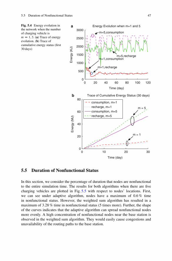
5.5 Duration of Nonfunctional Status 47

Fig. 5.4 Energy evolution inthe network when the numberof charging vehicle ism D 1; 5. (a) Trace of energyevolution. (b) Trace ofcumulative energy status (first30 days)

0 20 40 60 80 100 1200

500

1000

1500

2000

2500

3000Energy Evolution when m=1 and 5

Time (day)

Ene

rgy

(KJ)

m=1,consumption

m=1,recharge

m=5,recharge

m=5,consumption

a

0 10 20 300

20

40

60

80Trace of Cumulative Energy Status (30 days)

Time (day)

Ene

rgy

(MJ)

consumption, m=1recharge, m=1consumption, m=5recharge, m=5

m = 1

m = 5

b

5.5 Duration of Nonfunctional Status

In this section, we consider the percentage of duration that nodes are nonfunctionalto the entire simulation time. The results for both algorithms when there are fivecharging vehicles are plotted in Fig. 5.5 with respect to nodes’ locations. First,we can see under adaptive algorithm, nodes have a maximum of 0.6 % timein nonfunctional status. However, the weighted sum algorithm has resulted in amaximum of 3.28 % time in nonfunctional status (5 times more). Further, the shapeof the curves indicates that the adaptive algorithm can spread nonfunctional nodesmore evenly. A high concentration of nonfunctional nodes near the base station isobserved in the weighted sum algorithm. They would easily cause congestions andunavailability of the routing paths to the base station.


0100

200

0

100

2000

2

4

X−Axis (m)

Percentage of Nonfunctional Time − Weighted Sum Algorithm

Y−Axis (m)

Max value = 3.28%

a

0100

200

0

100

2000

2

4

X−Axis (m)

Percentage of Nonfunctional Time − Adaptive Algorithm

Y−Axis (m)

Max value = 0.6%

b

Fig. 5.5 Evaluation of percentage time that nodes are nonfunctional. (a) Weighted-sum algorithm.(b) Adaptive algorithm

5.6 Data Collection Latency

Data collection latency depends on whether a routing path is available. To success-fully transmit all sensed data to the base station timely, all the nodes on the routingpaths should be functional. If a node depletes battery energy and no alternate routeis available, the packets will be buffered at sensors until the path is restored bythe charging vehicle. Shortest path trees are formed using the Dijsktra’s algorithmrooted at the base station. Figure 5.6 shows the average data collection delay overthe entire simulation time. Since the adaptive algorithm has higher capability ofhandling nonfunctional nodes than the weighted sum algorithm, 45 % less data delayis achieved with the adaptive algorithm.

5.8 Charging Vehicle’s Moving Energy Cost 49

Fig. 5.6 Evaluation of datacollection delay

1 2 3 4 50

20

40

60

80

100Evaluation of Average Data Collection Latency

Number of Charging Vehicles m

Dat

a C

olle

ctio

n La

tenc

y (m

ins)

Weighted−sum Algorithm

Adaptive Algorithm

5.7 Overhead of Node Status Collection Protocol

The communication overhead represents the energy consumed for transmittingall types of control packets, e.g., head selection, status request/report, emergencyrequest/report and head notification packets. Figure 5.7 shows the evolution ofcommunication energy overhead during 4 months simulation time. First, comparedto the energy cost for transmitting sensed data, the overhead in the communicationprotocol is not significant. Its energy consumption is around 10 mJ/day comparedto at least 8.64 J/day for transmitting sensed data packets. Second, there is a certainamount of overhead during the network setup phase (around 40–60 mJ/day per node)due to the head selection process. During the operation, when a head node is lowon energy, it sends out a head notification packet to appoint a new head node. Thehead selection would then propagate up through the hierarchy. This process alsocontributes to the overhead from 20 to 120 days time. Further, for different numberof charging vehicles, more communication overhead is observed when the numberof charging vehicles is not enough (m D 1; 2). In this case, recharge requests andhead re-selection are performed more often than m D 3–4 so higher communicationoverhead is expected for fewer charging vehicles.

5.8 Charging Vehicle’s Moving Energy Cost

We now examine the moving energy cost on the charging vehicles. Since thevehicles also consume energy while moving, one of the goals is to design rechargescheduling algorithms that can provide extra savings in the charging vehicle’smoving cost. Figure 5.8 shows the average energy cost per vehicle for the weightedsum and adaptive algorithms. It is interesting to see that when m D 1–3, the


Fig. 5.7 Evaluation ofenergy overhead of nodestatus reporting protocol

0 20 40 60 80 100 1200

20

40

60

80Energy Overhead from Node Status Reporting


Ene

rgy

Ove

rhea

d (m

J)

m=1

m=2

m=3

m=4

Fig. 5.8 Evaluation ofcharging vehicle’s movingcost for weighted sum andadaptive algorithms

1 2 3 4 50

200

400

600

800

1000

1200Evaluation of moving energy cost

Number of Charging Vehicles m

Mov

ing

Ene

rgy

Cos

t (K

J)


Adaptive Algorithm

weighted sum algorithm is more energy efficient than the adaptive algorithm. Thisis because that when the number of vehicles is not enough (m D 1–3) to supportperpetual operation, there are always energy requests so the weighted sum algorithmselects the nearest node with the least lifetime. When m D 4–5, the energyrequest becomes sporadic during operations. The weighted sum algorithm that onlyrecharges the node with the least weighted value might make the vehicle movelong distance. In contrast, the adaptive algorithm partitions the network into smallerregions so the vehicles have much shorter moving distance in each recharge. Thisreduces the moving cost significantly.

5.9 Comparison with Static Optimization Approach 51

5.9 Comparison with Static Optimization Approach

Finally, we compare the performance of the two algorithms with the static opti-mization approach used in [5]. In the static approach, a charging vehicle selectsnodes with energy less than the normal recharge threshold and calculates theshortest recharging tour among the selected nodes. We first compare the percentageof nonfunctional nodes shown in Fig. 5.9. The number of nonfunctional nodes ismuch higher for the static approach. For m D 1, there are 60 % nonfunctionalnodes whereas the weighted-sum and adaptive algorithms result in less than 30 %nonfunctional nodes. This is because the static approach does not consider nodelifetime and only follows a pre-computed sequence to recharge nodes.

Next, we look at the emergency response time which is the duration from a nodereports emergency until it is recharged. Shorter response time means the chargingvehicle can respond rapidly to emergencies. Figure 5.10 shows the average responsetime to emergencies when the number of nodes varies from 250 to 500. We cansee while the adaptive algorithm takes around 4 and 14 h (for N D 250 and 500,respectively), the static approach takes much longer time (around 24 and 45 h). Thereason of such improvement is that we have differentiated emergency and normalrecharging operations. However, in [5], nodes are treated regardless of their lifetime.This would incur extended recharge delay for some emergent nodes and causebattery depletion. As a result, the static approach degrades fast as the network sizeincreases.

Fig. 5.9 Comparing thepercentage of nonfunctionalnodes between differentschemes

0 20 40 60 80 100 1200

20

40

60

80


Per

cent

age(

%)

Nonfunctional nodes of different schemes

Static Approach


Adaptive Algorithm


Fig. 5.10 Comparingemergency response timebetween different schemes

N=250 N=5000

20

40

60

Evaluation of emergency response time

Number of Nodes

Ave

rage

Res

pons

e T

ime

(h) Static Approach

Weighted−sum AlgorithmAdaptive Algorithm

5.10 Summary

This chapter provides the performance evaluation results of some important perfor-mance metrics in WRSNs. From comparisons between the presented algorithmsand optimal solution, we can see that the adaptive algorithm can achieve veryclose approximation to the optimal solution and provide an additional 10 % costsaving over the weighted sum algorithm. With more sophisticated algorithm design,the adaptive algorithm provides much better performance than the weighted sumalgorithm in reducing the number of nonfunctional nodes, data collection delay andmoving cost. The communication overhead of the node status reporting protocol isalso examined. It indicates that the energy overhead is negligible compared to theenergy consumed for transmitting data packets. These results can offer insights fordesigning real WRSNs.

References

1. Panasonic Ni-MH battery handbook, “http://www2.renovaar.ee/userfiles/Panasonic_Ni-MH_Handbook.pdf”.

2. T.H. Cormen, C. E. Leiserson, R. L. Rivest and C. Stein, Introduction to Algorithms, MIT Press,2001.

3. Battery Calculator, “http://www.evsource.com/battery_calculator.php.”4. TI CC2430 Datasheet, “http://www.ti.com/product/cc2430.”5. M. Zhao, J. Li and Y. Yang, “Joint mobile energy replenishment and data gathering in wireless

rechargeable sensor networks,” IEEE Transactions on Mobile Computing, vol. 13, no. 12,pp. 2689–2705, 2014.



http://www.evsource.com/battery_ calculator.php

http://www.ti.com/product/cc2430

Chapter 6Conclusions

In this book, we discuss how to apply the novel wireless charging technologyto traditional wireless sensor networks to provide perpetual network operation.First, we provide a comprehensive literature review on the state-of-the-art wirelesscharging techniques and their impacts. Then we introduce the network architecturefor wireless rechargeable sensor networks by describing the functionality of networkcomponents and their features. We analyze several important theoretical aspects andderive important principles for the perpetual operation condition to hold.

We provide a distributed communication protocol for collecting node statusin a scalable manner. We further examine the recharge scheduling problem foremergency and normal node recharge. To recharge multiple emergent nodes, weshow how to formulate the problem into an Orienteering problem and describea solution based on dynamic programming. For normal recharge, we give twoscheduling algorithms. The first algorithm uses a weighted value to account formoving cost and node’s lifetime. The second algorithm partitions the networkadaptively, forms Capacitated Minimum Spanning Trees for each charging vehicle,and finally improves the recharge route. We also present extensive simulation resultsto compare the performance between the two algorithms in different criteria.

With this book, we hope to shed some light on the current research statusof wireless rechargeable sensor networks, and those characterizations of variousdesigns in the book could inspire future research. Another aim of this book is toprovide a solution to tackle the energy issues in many distributed systems. We expectreaders to find this book useful and supportive when facing many challenges indesigning future wireless sensor networks and distributed systems.


53

Glossary

AAdaptive network partition, 37–41Area, 1, 9, 10, 17, 18, 21, 22

BBase station, 5, 9, 10, 14, 28, 29, 31, 33, 34,

37, 43, 47, 48

CCapacitated Minimum Spanning Tree, 33–39Charging vehicle, 5, 9–15, 17–22, 25, 28–38,

41, 43–45, 47–50

DDynamic programming, 27, 41, 53

EElectromagnetic radiation, 3–4Emergency, 10, 18, 21–22, 25–28, 38, 41, 49,

51–53Energy neutral, 11–13, 15Esau-Williams (EW) algorithm, 35–37, 41

HHead election, 17–19, 21, 22Head node, 9, 10, 17–22, 49Head notification, 17, 49

KK-means, 33Knapsack problem, 26, 27

MMagnetic resonant coupling, 3–5

NNode lifetime, 1, 11, 13-15, 17

OOrienteering problem (OP), 25–28, 41, 53

PPrioritized recharge, 28, 38Proxy, 10, 18, 21, 22, 25

RRecharge threshold, 10, 11, 14–15, 18, 20, 21,

43, 51

SStatus report, 17–22, 50, 52Status request, 10, 17–22, 49

© The Author(s) 2015Y. Yang, C. Wang, Wireless Rechargeable Sensor Networks, SpringerBriefsin Electrical and Computer Engineering, DOI 10.1007/978-3-319-17656-7

55

56 Glossary

TTraveling salesmen problem (TSP), 30, 38, 41

VVehicle routing problem, 30, 41

WWeighted-sum algorithm, 31–33, 46, 48Wireless charging, 2–5, 53Wireless rechargeable sensor network

(WRSN), 2, 4, 5, 9, 11–15, 53Wireless sensor network (WSNs), 1–5, 53

yuanyuan˜yang cong˜wang wireless rechargeable sensor …

Documents