1

Zero-Delay Sequential Transmission of MarkovSources over Burst Erasure Channels

Farrokh Etezadi, Ashish Khisti and Mitchell Trott

Abstract—A setup involving zero-delay sequential transmissionof a vector Markov source over a burst erasure channel is studied.A sequence of source vectors is compressed in a causal fashion atthe encoder, and the resulting output is transmitted over a bursterasure channel. The destination is required to reconstruct eachsource vector with zero-delay, but those source sequences that areobserved either during the burst erasure, or in the interval oflength W following the burst erasure need not be reconstructed.The minimum achievable compression rate is called the rate-recovery function. We assume that each source vector is sampledi.i.d. across the spatial dimension and from a stationary, first-order Markov process across the temporal dimension.

For discrete sources the case of lossless recovery is considered,and upper and lower bounds on the rate-recovery function areestablished. Both these bounds can be expressed as the rate forpredictive coding, plus a term that decreases at least inverselywith the recovery window length W . For Gauss-Markov sourcesand a quadratic distortion measure, upper and lower bounds onthe minimum rate are established when W = 0. These boundsare shown to coincide in the high resolution limit. Finally anothersetup involving i.i.d. Gaussian sources is studied and the rate-recovery function is completely characterized in this case.

Index Terms—Joint Source-Channel Coding, DistributedSource Coding, Gauss-Markov Sources, Kalman Filter, BurstErasure Channels, Multi-terminal Information Theory, Rate-distortion Theory.

I. INTRODUCTION

REal-time streaming applications require both the sequen-tial compression, and playback of multimedia frames

under strict latency constraints. Linear predictive techniquessuch as DPCM have long been used to exploit the sourcememory in such systems. However predictive coding schemesalso exhibit a significant level of error propagation in thepresence of packet losses [1]. In practice one must developtransmission schemes that satisfy both the real-time constraintsand are robust to channel errors.

There exists an inherent tradeoff between the underlyingtransmission-rate and the error-propagation at the receiverin all video streaming applications. Commonly used videocompression formats such as H.264/MPEG and HEVC use acombination of intra-coded and predictively-coded frames tolimit the amount of error propagation. The predictively-codedframes are used to improve the compression efficiency whereas

Manuscript submitted June 2013, revised December 2013.Farrokh Etezadi (fetezadi@comm.utoronto.ca) and Ashish Khisti

(akhisti@comm.utoronto.ca) are with the University of Toronto, Toronto,ON, Canada, Mitchell Trott was with HP Labs, Palo Alto, USA. This workwas supported by an NSERC Discovery Research Grant, a Hewlett-PackardInnovation Research Program award and an Ontario Early Research Award.This work was presented in parts at the 2012 IEEE Data CompressionConference and the 2012 Allerton Conference on Communication, Controland Computing.

the intra-coded frames limit the amount of error propagation.Other techniques including forward error correction codes [2],leaky DPCM [3] and distributed video coding [4] can also beused to trade off the transmission rate with error propagation.Despite this, such a tradeoff is not well understood even inthe case of a single isolated packet loss [5].

In this paper we study the information theoretic tradeoff be-tween the transmission rate and error propagation in a simplesource-channel model. We assume that the channel introducesan isolated erasure burst of a certain maximum length, sayB. The encoder observes a sequence of vector sources andcompresses them in a causal fashion. The decoder is requiredto reconstruct each source vector with zero delay, except thosethat occur during the error propagation window. The decodercan declare a don’t-care for all the source sequences that occurin this window. We assume that is period spans the duration ofthe erasure burst, as well an interval of length W immediatelyfollowing it. We study the minimum rate required R(B,W ),and define it as the rate-recovery function.

We first consider the case of discrete sources and losslessreconstruction and establish upper and lower bounds on theminimum rate. Both these bounds can be expressed as therate of the predictive coding scheme, plus an additionalterm that decreases at-least as H(s)/(W + 1) where H(s)denotes the entropy of the source symbol. Our lower boundis obtained through connection to a certain multi-terminalsource coding problem that captures the tension in encodinga source sequence during the error-propagation period, andoutside it. The upper bound is based on a natural random-binning scheme. We also consider the case of Gauss-Markovsources and a quadratic distortion measure. We again establishupper and lower bounds on the minimum rate when W = 0,i.e., when instantaneous recovery following the burst erasureis imposed. We observe that our upper and lower boundscoincide in the high resolution limit, thus establishing therate-recovery function in this regime. Finally we consider adifferent setup involving i.i.d. Gaussian sources, and a specialrecovery constraint, and obtain an exact characterization of therate-recovery function in this special case. Many of our resultsalso naturally extend to the case when the channel introducesmultiple erasure bursts.

The remainder of the paper is organized as follows. Wediscuss related literature in Section II. The problem setup isdescribed in Section III and a summary of the main results isprovided in Section IV. We treat the case of discrete sourcesand lossless recovery in Section V and establish upper andlower bounds on the minimum rate. The optimality of binningfor the special case of symmetric sources and memorylessencoders is established in Section VI. In Section VII we

2

consider the case of Gauss-Markov source with a quadraticdistortion constraint. Section VIII studies another setup in-volving independent Gaussian sources and a sliding windowrecovery constraint, where an exact characterization of theminimum rate is obtained. Conclusions appear in Section IX.

Notations: Throughout this paper we represent the Eu-clidean norm operator by || · || and the expectation operatorby E[·]. The notation “log” is used for the binary logarithm,and rates are expressed in bits. The operations H(.) and h(.)denote the entropy and the differential entropy, respectively.The “slanted sans serif” font a and the normal font a repre-sent random variables and their realizations respectively. Thenotation ani = ai,1, . . . , ai,n represents a length-n sequenceof symbols at time i. The notation [f ]ji for i < j representsfi, fi+1, . . . , fj .

II. RELATED WORKS

Problems involving real-time coding and compression havebeen studied from many different perspectives in relatedliterature. The compression of a Markov source, with zeroencoding and decoding delays, was studied in an early work byWitsenhausen [6]. In this setup, the encoder must sequentiallycompress a (scalar) Markov source and transmit it over an idealchannel. The decoder must reconstruct the source symbolswith zero-delay and under an average distortion constraint. Itwas shown in [6] that for a k-th order Markov source model,an encoding rule that only depends on the k most recent sourcesymbols, and the decoder’s memory, is sufficient to achieve theoptimal rate. Similar structural results have been obtained in anumber of followup works, see e.g., [7] and references therein.The authors in [8] considered real-time communication ofa memoryless source over memoryless channels, with orwithout the presence of unit-delay feedback. The encodingand decoding is sequential with a fixed finite lookahead atthe encoder. The authors propose conditions under whichsymbol-by-symbol encoding and decoding, without lookahead,is optimal and more generally characterize the optimal encoderas a solution to a dynamic programming problem.

In another line of work, the problem of sequential codingof correlated vector sources in a multi-terminal source codingframework was introduced by Viswanathan and Berger [9].In this setup, a set of correlated sources must be sequentiallycompressed by the encoder, whereas the decoder at each stageis required to reconstruct the corresponding source sequence,given all the encoder outputs up to that time. It is noted in [9]that the correlated source sequences can model consecutivevideo frames and each stage at the decoder maps to sequentialreconstruction of a particular source frame. This setup is anextension of the well-known successive refinement problemin source coding [10]. In followup works, in reference [11]the authors consider the case where the encoders at each timehave access to previous encoder outputs rather than previoussource frames. Reference [12] considers an extension wherethe encoders and decoders can introduce non-zero delays. Allthese works assume ideal channel conditions. Reference [13]considers an extension of [9] where at any given stage thedecoder has either all the previous outputs, or only the present

output. A robust extension of the predictive coding schemeis proposed and shown to achieve the minimum sum-rate.However this setup does not capture the effect of packet lossesover a channel, where the destination has access to all thenon erased symbols. To our knowledge, only reference [3]considers the setting of sequential coding over a randompacket erasure channel. The source is assumed to be Gaussian,spatially i.i.d. and temporally autoregressive. A class of linearpredictive coding schemes is studied and an optimal schemewithin this class, with respect to the excess distortion ratio met-ric is proposed. Our proposed coding scheme is qualitativelydifferent from [3], [13] and involves a random binning basedapproach, which is inherently robust to the side-informationat the decoder.

In other related works, the joint source-channel coding of avector Gaussian source over a vector Gaussian channel withzero reconstruction delay has also been extensively studied.While optimal analog mappings are not known in general,a number of interesting approaches have been proposed ine.g. [14], [15] and related references. Reference [16] studiesthe problem of sequential coding of the scalar Gaussian sourceover a channel with random erasures. In [5], the authorsconsider a joint source-channel coding setup and propose theuse of distributed source coding to compensate the effect ofchannel losses. However no optimality results are presented forthe proposed scheme. Sequential random binning techniquesfor streaming scenarios have been proposed in e.g. [17], [18]and the references therein.

To the best of our knowledge, there has been no prior workthat studies an information theoretic tradeoff between error-propagation and compression efficiency in real-time streamingsystems.

III. PROBLEM STATEMENT

In this section we introduce our source and channel modelsand the associated definition of the rate-recovery function.

We assume that the communication spans the intervali ∈ [−1,L]. At each time i, a source vector sni is sampled,whose symbols are drawn independently across the spatialdimension, and from a first-order Markov chain across thetemporal dimension, i.e.,

Pr( sni = sni | sni−1 = sni−1, sni−2 = sni−2, . . . , sn−1 = sn−1)

=

n∏k=1

p1(si,k|si−1,k), 0 ≤ i ≤ L. (1)

The underlying random variables si constitute a time-invariant, stationary and a first-order Markov chain with acommon marginal distribution denoted by ps(·) over an al-phabet S. The sequence sn−1 is sampled i.i.d. from ps(·) andrevealed to both the encoder and decoder before the start of thecommunication. It plays the role of a synchronization frame.

A rate-R encoder computes an index fi ∈ [1, 2nR] at timei, according to an encoding function

fi = Fi(sn−1, s

n0 , ..., s

ni

), 0 ≤ i ≤ L. (2)

Note that the encoder in (2) is a causal function of the sourcesequences. A memoryless encoder satisfies Fi(·) = Fi(sni )

3

sn−1 sn0

f0

f0

sn0

sn1

f1

f1

sn1

sn2

f2

f2

sn2

snj−1

fj−1

fj−1

snj−1

snj

fj

?

−

snj+1

fj+1

?

−

snj+B−1

fj+B−1

?

−

snj+B

fj+B

fj+B

−

snj+B+W−1

fj+B+W−1

fj+B+W−1

−

snj+B+W

fj+B+W

fj+B+W

snj+B+W

snj+B+W+1

fj+B+W+1

fj+B+W+1

snj+B+W+1

Erased Not to be recovered

Error Propagation Window

Fig. 1: Problem Setup: The encoder output fi is a function of all the past source sequences. The channel introduces a bursterasure of length up to B. The decoder produces sni upon observing the channel outputs up to time i. As indicated, the decoderis not required to produce those source sequences that are observed either during the burst erasure, or a period of W followingit. The first sequence, sn−1 is a synchronization frame available to both the source and destination.

i.e., the encoder does not use the knowledge of the pastsequences. Naturally a memoryless encoder is very restrictive,and we will only use it to establish some special results.

The channel takes each fi as input and either outputs gi = fior an erasure symbol i.e., gi = ?. We consider the class ofburst erasure channels. For some particular j ≥ 0, it introducesa burst erasure such that gi = ? for i ∈ j, j+1, ..., j+B′−1and gi = fi otherwise i.e.,

gi =

?, i ∈ [j, j + 1, . . . , j +B′ − 1]

fi, else,(3)

where the burst length B′ is upper bounded by B.Upon observing the sequence gii≥0, the decoder is re-

quired to reconstruct each source sequence with zero delayi.e.,

sni = Gi(g0, g1, . . . , gi, sn−1), i /∈ j, . . . , j +B′ +W − 1

(4)

where sni denotes the reconstruction sequence and j denotesthe time at which burst erasure starts in (3). The destination isnot required to produce the source vectors that appear eitherduring the burst erasure or in the period of length W followingit. We call this period the error propagation window. Fig. 1provides a schematic of the causal encoder (2), the channelmodel (3), and the decoder (4).

A. Rate-Recovery Function

We define the rate-recovery function under lossless andlossy reconstruction constraints.

1) Lossless Rate-Recovery Function: We first consider thecase when the reconstruction in (4) is required to be lossless.We assume that the source alphabet is discrete and the entropyH(s) is finite. A rate RL(B,W ) is feasible if there exists asequence of encoding and decoding functions and a sequenceεn that approaches zero as n→∞ such that, Pr(sni 6= sni ) ≤εn for all source sequences reconstructed as in (4). We seekthe minimum feasible rate RL(B,W ), which is the lossless

TABLE I: Summary of notation used in the paper.

SourceParameters

Source Symbol sSource Reproduction s

Temporal Correlation Coefficientof Gauss-Markov Source Model ρ

ChannelParameters

Channel Input fChannel Output g

Maximum Burst Length BGuard Length between Consecutive Bursts L

SystemParameters

Length of Source Sequences nCommunication Duration LRecovery Window Length W

PerformanceMetrics

Rate RAverage Distortion D

rate-recovery function. In this paper, we will focus on infinite-horizon case, R(B,W ) = limL→∞RL(B,W ), which will becalled the rate-recovery function for simplicity.

2) Lossy Rate-Recovery Function: We also consider thecase where reconstruction in (4) is required to satisfy anaverage distortion constraint:

lim supn→∞

E

[1

n

n∑k=1

d(si,k, si,k)

]≤ D (5)

for some distortion measure d : R2 → [0,∞). The rate Ris feasible if a sequence of encoding and decoding functionsexists that satisfies the average distortion constraint. The min-imum feasible rate RL(B,W,D), is the lossy rate-recoveryfunction. The study of lossy rate-recovery function for thegeneral case appears to be quite challenging. In this paperwe will focus on the class of Gaussian-Markov sources, withquadratic distortion measure, i.e. d(s, s) = (s− s)2, where theanalysis simplifies. We will again focus on infinite-horizoncase, R(B,W,D) = limL→∞RL(B,W,D) which we simplycall the rate-recovery function. Table I summarizes the notationused throughout the paper.

Remark 1. Note that our proposed setup only considers a

4

single burst erasure during the entire duration of communi-cation. When we consider lossless recovery at the destinationour results immediately extend to channels involving multi-ple burst erasures with a certain guard interval separatingconsecutive bursts. When we consider Gauss-Markov sourceswith a quadratic distortion measure, we will explicitly treatthe channel with multiple burst erasures and compare theachievable rates with that of a single burst erasure channel.

B. Practical Motivation

Note that our setup assumes that the size of both thesource frames and channel packets is sufficiently large. Arelevant application for the proposed setup is video streaming.Video frames are generated at a rate of approximately 60 Hzand each frame typically contains several hundred thousandpixels. The inter-frame interval is thus ∆s ≈ 17 ms. Supposethat the underlying broadband communication channel has abandwidth of Ws = 2.5 MHz. Then in the interval of ∆s

the number of symbols transmitted using ideal synchronousmodulation is N = 2∆sWs ≈ 84, 000. Thus the block lengthbetween successive frames is sufficiently long that capacityachieving codes could be used and the erasure model andlarge packet sizes is justified. The assumption of spatially i.i.d.frames could reasonably approximate the video innovationprocess generated by applying suitable transform on originalvideo frames. Such models have been also used in earlierworks e.g., [3], [9], [11]–[13].

Possible applications of the burst loss model consideredin our setup include fading wireless channels and congestionin wired networks. We note that the present paper does notconsider a statistical channel model but instead considers aworst case channel model. As mentioned before even the effectof such a single burst loss has not been well understood inthe video streaming setup and therefore our proposed setupis a natural starting point. Furthermore while the statisticalmodels are used to capture the typical behaviour of channelerrors, the atypical behaviour is often modelled (see e.g., [19,Sec. 6.10]) using a worst-case approach. Therefore in low-latency applications where the local channel dynamics arerelevant such models are often used (see e.g., [20]–[23]).Finally we note that earlier works (see e.g., [3]) that considerstatistical channel models, also ultimately simplify the systemby analyzing the effect of each burst erasure separately insteady state.

IV. MAIN RESULTS

We summarize the main results of this paper. We notein advance that throughout the paper, the upper bound onthe rate-recovery function indicates the rate achievable by aproposed coding scheme and the lower bound corresponds toa necessary condition that the rate-recovery function of anyfeasible coding scheme has to satisfy. Section IV-A treats thelossless rate-recovery function and presents lower and upperbounds in Theorem 1. Corollary 2 presents the lossless rate-recovery function for a special case of symmetric sources,when restricted to memoryless encoders. Section IV-B treatsthe lossy rate-recovery function for the class of Gauss-Markov

sources. Prop. 1 presents a lower bound, whereas Prop. 2 andProp. 3 present upper bounds on lossy rate-recovery functionfor the single and multiple burst erasure channel modelsrespectively. Our bounds coincide in the high resolution limit,as stated in Corollary 3. Finally Section IV-C treats anothersetup involving independent Gaussian sources, with a slidingwindow recovery constraint, and establishes the associatedrate-recovery function.

A. Lossless Rate-Recovery Function

Theorem 1. (Lossless Rate-Recovery Function) For the sta-tionary, first-order Markov, discrete source process, the loss-less rate-recovery function satisfies the following upper andlower bounds: R−(B,W ) ≤ R(B,W ) ≤ R+(B,W ), where

R+(B,W )=H(s1|s0) +1

W + 1I(sB ; sB+1|s0), (6)

R−(B,W )=H(s1|s0) +1

W + 1I(sB ; sB+W+1|s0). (7)

Notice that the upper and lower bounds (6) and (7) coincidefor W = 0 and W → ∞, yielding the rate-recovery functionin these cases. We can interpret the term H(s1|s0) as theamount of uncertainty in si when the past sources are perfectlyknown. This term is equivalent to the rate associated with idealpredictive coding in absence of any erasures. The second termin both (6) and (7) is the additional penalty that arises dueto the recovery constraint following a burst erasure. Noticethat this term decreases at-least as H(s)/(W + 1), thus thepenalty decreases as we increase the recovery period W . Notethat the mutual information term associated with the lowerbound is I(sB ; sB+W+1|s0) while that in the upper bound isI(sB ; sB+1|s0). Intuitively this difference arises because in thelower bound we only consider the reconstruction of snB+W+1

following an erasure bust in [1, B] while, as explained below inCorollary 1 the upper bound involves a binning based schemethat reconstructs all sequences (snB+1, . . . , s

nB+W+1) at time

t = B +W + 1.A proof of Theorem 1 is provided in Section V. The lower

bound involves a connection to a multi-terminal source codingproblem. This model captures the different requirements im-posed on the encoder output following a burst erasure and inthe steady state. The following Corollary provides an alternateexpression for the achievable rate and makes the connectionto the binning technique explicit.

Corollary 1. The upper bound in (6) is equivalent to thefollowing expression

R+(B,W ) =1

W + 1H(sB+1, sB+2, . . . , sB+W+1|s0). (8)

The proof of Corollary 1 is provided in Appendix A.We make several remarks. First, the entropy term in (8)is equivalent to the sum-rate constraint associated with theSlepian-Wolf coding scheme in simultaneously recoveringsnB+1, s

nB+2, . . . , s

nB+W+1 when sn0 is known. Note that due

to the stationarity of the source process, the rate expression in

5

(8) suffices for recovering from any burst erasure of lengthup to B, spanning an arbitrary interval. Second, note thatin (8) we amortize over a window of length W + 1 assnB+1, . . . , s

nB+W+1 are recovered simultaneously at time

t = B+W +1. Note that this is the maximum window lengthover which we can amortize due to the decoding constraint.Third, the results in Theorem 1 immediately apply when thechannel introduces multiple bursts with a guard spacing of atleast W + 1. This property arises due to the Markov natureof the source. Given a source sequence at time i, all thefuture source sequences snt t>i are independent of the pastsnt t<i when conditioned on sni . Thus when a particularsource sequence is reconstructed at the destination, the decoderbecomes oblivious to past erasures. Finally, while the resultsin Theorem 1 are stated for the rate-recovery function over aninfinite horizon, upon examining the proof of Theorem 1, itcan be verified that both the upper and lower bounds hold forthe finite horizon case, i.e. RL(B,W ), when L ≥ B +W .

A symmetric source is defined as a Markov source such thatthe underlying Markov chain is also reversible i.e., the randomvariables satisfy (s0, . . . , sl)

d= (sl, . . . , s0), where the equality

is in the sense of distribution [24]. Of particular interest to usis the following property satisfied for each t:

pst+1,st(sa, sb) = pst−1,st(sa, sb), ∀sa, sb ∈ S (9)

i.e., we can “exchange” the source pair (snt+1, snt ) with

(snt−1, snt ) without affecting the joint distribution. An exam-

ple of a symmetric source is the binary symmetric source:snt = snt−1 ⊕ znt , where znt t≥0 is an i.i.d. binary sourceprocess (in both temporal and spatial dimensions) with themarginal distribution Pr(zt,i = 0) = p, the marginal distribu-tion Pr(st,i = 0) = Pr(st,i = 1) = 1

2 and ⊕ denotes modulo-2addition.

Corollary 2. For the class of symmetric Markov sources thatsatisfy (9), the lossless rate-recovery function when restrictedto the class of memoryless encoders i.e., fi = Fi(sni ), is givenby

R(B,W ) =1

W + 1H(sB+1, sB+2, . . . , sB+W+1|s0). (10)

The proof of Corollary 2 is presented in Section VI. Theconverse is obtained by again using a multi-terminal sourcecoding problem, but obtaining a tighter bound by exploitingthe memoryless property of the encoders and the symmetricstructure (9).

B. Gauss-Markov Sources

We study the lossy rate-recovery function when sni is sampled i.i.d. from a zero-mean Gaussian distribution,N (0, σ2

s), along the spatial dimension and forms a first-orderMarkov chain across the temporal dimension i.e.,

si = ρsi−1 + ni (11)

where ρ ∈ (0, 1) and ni ∼ N (0, σ2s(1 − ρ2)). Without loss

of generality we assume σ2s = 1. We consider the quadratic

distortion measure d(si, si) = (si − si)2 between the source

symbol si and its reconstruction si. In this paper we focuson the special case of W = 0, where the reconstruction mustbegin immediately after the burst erasure. We briefly remarkabout the case when W > 0 at the end of Section VII-B.As stated before unlike the lossless case, the results of Gauss-Markov sources for single burst erasure channels do not readilyextend to the multiple burst erasures case. Therefore, we treatthe two cases separately.

1) Channels with Single Burst Erasure: In this channelmodel, as stated in (3), we assume that the channel can intro-duce a single burst erasure of length up to B during the trans-mission period. Define RGM-SE(B,D) , R(B,W = 0, D) asthe lossy rate-recovery function of Gauss-Markov sources withsingle burst erasure channel model.

Proposition 1 (Lower Bound–Single Burst). The lossy rate-recovery function of the Gauss-Markov source for single bursterasure channel model when W = 0 satisfies

RGM-SE(B,D) ≥ R−GM-SE(B,D) ,

1

2log

(Dρ2 + 1− ρ2(B+1) +

√∆

2D

)(12)

where ∆ , (Dρ2 + 1− ρ2(B+1))2 − 4Dρ2(1− ρ2B).

The proof of Prop. 1 is presented in Section VII-A. Theproof considers the recovery of a source sequence snt , given aburst erasure in the interval [t−B, t−1] and extends the lowerbounding technique in Theorem 1 to incorporate the distortionconstraint.

Proposition 2 (Upper Bound–Single Burst). The lossy rate-recovery function of the Gauss-Markov source for single bursterasure channel model when W = 0 satisfies

RGM-SE(B,D) ≤ R+GM-SE(B,D) , I(st; ut|st−B) (13)

where ut , st + zt, and zt is sampled i.i.d. from N (0, σ2z).

Also st−B , st−B + e and e ∼ N(0,Σ(σ2

z)/(1− Σ(σ2z)))

with

Σ(σ2z) ,

1

2

√(1− σ2

z)2(1− ρ2)2 + 4σ2z(1− ρ2) +

1− ρ2

2(1− σ2

z),

(14)

is independent of all other random variables. The test channelnoise σ2

z > 0 is chosen to satisfy[1

σ2z

+1

1− ρ2B(1− Σ(σ2z))

]−1

≤ D. (15)

This is equivalent to σ2z satisfying

E[(st − st)

2]≤ D, (16)

where st denotes the minimum mean square estimate (MMSE)of st from st−B , ut.

The following alternative rate expression for the achievablerate in Prop. 2, provides a more explicit interpretation of the

6

0 0.2 0.4 0.6 0.8 10

0.2

0.4

0.6

0.8

1

ρ

Rate

Bits/S

ym

bol

Upper Bound

Lower Bound

D = 0.3B=1

D = 0.2B=1

D = 0.2B=2

D = 0.3B=2

Fig. 2: Lower and upper bounds of lossy rate-recoveryfunction RGM-SE(B,D) versus ρ for D = 0.2, D = 0.3and B = 1, B = 2.

0 0.2 0.4 0.6 0.8 10

0.5

1

1.5

2

2.5

3

3.5

D

Rate

Bits/S

ym

bol

Upper Bound

Lower Bound

ρ = 0.9

B=2ρ = 0.9

B=1

ρ = 0.7

B=2 ρ = 0.7

B=1

Fig. 3: Lower and upper bounds of lossy rate-recoveryfunction RGM-SE(B,D) versus D for ρ = 0.9, ρ = 0.7and B = 1, B = 2.

coding scheme.

R+GM-SE(B,D) = lim

t→∞I(st; ut|[u]t−B−1

0 ) (17)

where the random variables ut are obtained using the sametest channel in Prop. 2. Notice that the test channel noiseσ2z > 0 is chosen to satisfy E

[(st − st)

2]≤ D where st

denotes the MMSE of st from [u]t−B−10 , ut in steady state,

i.e. t→∞. Notice that (17) is based on a quantize and binningscheme when the receiver has side information sequencesun0 , . . . , unt−B−1. The proof of Prop. 2 which is presentedin Section VII-B also involves establishing that the worst caseerasure pattern during the recovery of snt spans the interval[t − B − 1, t − 1]. The proof is considerably more involvedas the reconstruction sequences unt do not form a Markovchain.

As we will show subsequently, the upper and lower boundsin Prop. 1 and Prop. 2 coincide in the high resolution limit.Numerical evaluations suggest that the bounds are close fora wide range of parameters. Fig. 2 and Fig. 3 illustrate somesample comparison plots.

2) Channels with Multiple Burst Erasures: We also con-sider the case where the channel can introduce multiple bursterasures, each of length no greater than B and with a guardinterval of length at-least L separating consecutive bursts. Theencoder is defined as in (2). We again only consider the casewhen W = 0. Upon observing the sequence gii≥0, thedecoder is required to reconstruct each source sequence withzero delay, i.e.,

sni = Gi(g0, g1, . . . , gi, sn−1), whenever gi 6= ? (18)

such that the reconstructed source sequence sni satisfies anaverage mean square distortion of D. The destination is notrequired to produce the source vectors that appear during anyof the burst erasures. The rate R(L,B,D) is feasible if a se-quence of encoding and decoding functions exists that satisfiesthe average distortion constraint. The minimum feasible rateRGM-ME(L,B,D), is the lossy rate-recovery function.

Proposition 3 (Upper Bound–Multiple Bursts). The lossyrate-recovery function RGM-ME(L,B,D) for Gauss-Markovsources over the multiple burst erasures channel satisfies thefollowing upper bound:

RGM-ME(L,B,D) ≤ R+GM-ME(L,B,D) ,

I(ut; st|st−L−B , [u]t−B−1t−L−B+1) (19)

where st−L−B = st−L−B + e, where e ∼ N (0, D/(1−D)).Also for any i, ui , si + zi and zi is sampled i.i.d. fromN (0, σ2

z) and the noise in the test channel, σ2z > 0 satisfies

E[(st − st)

2]≤ D (20)

and st denotes the MMSE estimate of st fromst−L−B , [u]t−B−1

t−L−B+1, ut.

The proof of Prop. 3 presented in Section VII-C is againbased on quantize-and-binning technique and involves charac-terizing the worst-case erasure pattern by the channel. Notealso that the rate expression in (19) depends on the minimumguard spacing L, the maximum burst erasure length B anddistortion D, but is not a function of time index t, as the testchannel is time invariant and the source process is stationary.An expression for computing σ2

z is provided in Section VII-C.While we do not provide a lower bound for RGM-ME(L,B,D)we remark that the lower bound in Prop. 1 also applies to themultiple burst erasures setup.

Fig. 4 provides numerical evaluation of the achievable ratefor different values of L. We note that even for L as smallas 4, the achievable rate in Prop. 3 is virtually identical tothe rate for single burst erasure in Prop. 2. This strikingly fastconvergence to the single burst erasure rate appears due tothe exponential decay in the correlation coefficient betweensource samples as time-lag increases.

3) High Resolution Regime: For both the single and multi-ple burst erasures models, the upper and lower bounds on lossyrate-recovery function for W = 0 denoted by R(L,B,D)coincide in the high resolution limit as stated below.

7

0.55 0.6 0.65 0.7 0.75 0.80.06

0.07

0.08

0.09

0.1

0.11

0.12

0.13

0.14

0.15

ρ

Rate

Bits/S

ym

bol

Multiple Erasure Bursts

Single Erasure Burst, Upper Bound

Single Erasure Burst, Lower Bound

L=3

L=1

L=2

L=4

(a) D = 0.8

0.55 0.6 0.65 0.7 0.75 0.8

0.25

0.3

0.35

0.4

0.45

ρ

Rate

Bits/S

ym

bol

Multiple Erasure Bursts

Single Erasure Burst, Upper Bound

Single Erasure Burst, Lower Bound

L=1

L=2

L=3

(b) D = 0.5

Fig. 4: Achievable rates for multiple burst erasures model for different values of guard length L separating burst erasurescomparing to single burst erasure. As L grows, the rate approaches the single erasure case. The lower bound for single erasurecase is also plotted for comparison (B = 1).

0.1 0.2 0.3 0.4 0.5 0.6 0.7 0.8 0.90

0.2

0.4

0.6

0.8

1

1.2

1.4

1.6

1.8

2

D

Rate

Bits/S

ym

bol

Single Erasure Burst, Upper Bound

Naive Wyner−Ziv

Single Erasure Burst, Lower Bound

ρ = 0.9

ρ = 0.8

Fig. 5: A comparison of achievable rates for the Gauss-Markovsource (B = 1).

Corollary 3. In the high resolution limit, the Gauss-Markovlossy rate-recovery function satisfies the following:

R(L,B,D) =1

2log

(1− ρ2(B+1)

D

)+ o(D). (21)

where limD→0 o(D) = 0.

The proof of Corollary 3 is presented in Section VII-D.It is based on evaluating the asymptotic behaviour of thelower bound in (12) and the upper bound in Prop. 3, in highresolution regime. Notice that the rate expression in (21) doesnot depend on the guard separation L. The intuition behindthis is as follows. In the high resolution regime, the outputof the test channel, i.e. ut, becomes very close to the originalsource st. Therefore the Markov property of the original sourceis approximately satisfied by these auxiliary random variablesand hence the past sequences are not required. The rate in (21)can also be approached by a Naive Wyner-Ziv coding scheme

that only makes use of the most recently available sequenceat the decoder [25]. The rate of this scheme is given by:

RNWZ(B,D) , I(st; ut|ut−B−1) (22)

where for each i, ui = si + zi and zi ∼ N (0, σ2z) and σ2

z

satisfies the following distortion constraint

E[(st − st)2] ≤ D (23)

where st is the MMSE estimate of st from ut−B−1, ut.Fig. 5 reveals that while the rate in (22) is near optimal

in the high resolution limit, it is in general sub-optimal whencompared to the rates in (19) when ρ = 0.9. As we decreaseρ, the performance loss associated with this scheme appearsto reduce.

C. Gaussian Sources with Sliding Window Recovery Con-straints

In this section we consider a specialized source model anddistortion constraint, where it is possible to improve upon thebinning based upper bound. Our proposed scheme attains therate-recovery function for this special case and is thus optimal.This example illustrates that the binning based scheme can besub-optimal in general.

1) Source Model: We consider a sequence of i.i.d. Gaussiansource sequences i.e., at time i, sni is sampled i.i.d. accordingto a zero mean unit variance Gaussian distribution N (0, 1),independent of the past sources. At each time we associate anauxiliary source

tni =(sni sni−1 . . . sni−K

)(24)

which is a collection of the past K + 1 source sequences. Notethat tni constitutes a first-order Markov chain. We will definea reconstruction constraint with the sequence tni .

2) Encoder: The (causal) encoder at time i generates anoutput given by fi = Fi(sn−1, . . . , s

ni ) ∈ [1, 2nR].

3) Channel Model: The channel can introduce a bursterasure of length up to B in an arbitrary interval [j, j+B−1].

8

si−2d2

si−1d1

sid0

titi−1ti−2ti−3

si−2

si−1

si

titi−1ti−2ti−3

sisi−1si−2si−3

timeii−1i−2i−3

Fig. 6: Schematic of the Gaussian sources with sliding windowrecovery constraints for K = 2. The source si, drawn aswhite circles, are independent sources and ti is defined asa collection of K + 1 = 3 most recent sources. The sourcesymbols along the diagonal lines are the same. The decoderat time i recovers si, si−1 and si−2 within distortions d0, d1

and d2, respectively where d0 ≤ d1 ≤ d2. In figure the colourdensity of the circle represents the amount of reconstructiondistortion.

4) Decoder: At time i the decoder is interested in re-producing a collection of past K + 1 sources1 within adistortion vector d = (d0, d1, · · · , dK) i.e., at time i thedecoder is interested in reconstructing (sni , . . . , s

ni−K) where

E[||sni−l − sni−l||2

]≤ ndl must be satisfied for l ∈ [0,K].

We assume throughout that d0 ≤ d1 ≤ . . . ≤ dK whichcorresponds to the requirement that the more recent sourcesequences must be reconstructed with a smaller average dis-tortion.

In Fig. 6, the source symbols si are shown as white circles.The symbols ti and ti are also illustrated for K = 2. Thedifferent shading for the sub-symbols in ti corresponds todifferent distortion constraints.

If a burst erasure spans the interval [j, j+B−1], the decoderis not required to output a reproduction of the sequences tnifor i ∈ [j, j +B +W − 1].

The lossy rate-recovery function denoted by R(B,W,d) isthe minimum rate required to satisfy these constraints.

Remark 2. One motivation for considering the above setup isthat the decoder might be interested in computing a functionof the last K + 1 source sequences at each time e.g.,, vi =∑Kj=0 α

jsi−j . A robust coding scheme, when the coefficientα is not known to the encoder is to communicate sni−j withdistortion dj at time i to the decoder.

Theorem 2. For the proposed Gaussian source model with anon-decreasing distortion vector d = (d0, . . . , dK) with 0 <

1In this section it is sufficient to assume that any source sequence with atime index j < −1 is a constant sequence.

di ≤ 1, the lossy rate-recovery function is given by

R(B,W,d) =1

2log

(1

d0

)+

1

W + 1

minK−W,B∑k=1

1

2log

(1

dW+k

). (25)

The proof of Theorem 2 is provided in Section VIII.The coding scheme for the proposed model involves usinga successive refinement codebook for each sequence sni toproduce B + 1 layers and carefully assigning the sequence oflayered codewords to each channel packet. A simple quantizeand binning scheme in general does not achieve the rate-recovery function in Theorem 2. A numerical comparisonof the lossy rate-recovery function with other schemes ispresented in Section VIII.

This completes the statement of the main results in thispaper.

V. GENERAL UPPER AND LOWER BOUNDS ON LOSSLESSRATE-RECOVERY FUNCTION

In this section we present the proof of Theorem 1. Inparticular, we show that the rate-recovery function satisfiesthe following lower bound.

R ≥ R−(B,W ) = H(s1|s0) +1

W + 1I(sB , sB+W+1|s0).

(26)

which is inspired by a connection to a multi-terminal sourcecoding problem introduced in Section V-A. Based on thisconnection, the proof of the lower bound in general form in(26) is presented in Section V-B. Then by proposing a codingscheme based on random binning, we show in Section V-Cthat the following rate is achievable.

R ≥ R+(B,W ) = H(s1|s0) +1

W + 1I(sB , sB+1|s0). (27)

A. Connection to Multi-terminal Source Coding Problem

We first present a multi-terminal source coding setup whichcaptures the tension inherent in the streaming setup. We focuson the special case when B = 1 and W = 1. At anygiven time j the encoder output fj must satisfy two objectivessimultaneously: 1) if j is outside the error propagation periodthen the decoder should use fj and the past sequences toreconstruct snj ; 2) if j is within the recovery period then fjmust only help in the recovery of a future source sequence.

Fig. 7 illustrates the multi-terminal source coding problemwith one encoder and two decoders that captures these con-straints. The sequences (snj , s

nj+1) are revealed to the encoder

and produces outputs fj and fj+1. Decoder 1 needs to recoversnj given fj and snj−1 while decoder 2 needs to recover snj+1

given snj−2 and (fj , fj+1). Thus decoder 1 corresponds to thesteady state of the system when there is no loss while decoder2 corresponds to the recovery immediately after an erasurewhen B = 1 and W = 1. We note in advance that the multi-terminal source coding setup does not directly correspond to

9

snj , snj+1

Encoder

Decoder1

snjfj

snj−1

Decoder2

snj+1

fj+1

snj−2

Fig. 7: Multi-terminal problem setup associated with ourproposed streaming setup when W = B = 1. The erasureat time t = j − 1 leads to two virtual decoders with differentside information as shown.

providing genie-aided side information in the streaming setup.In particular this setup does not account for the fact that theencoder has access to all previous source sequences and thedecoders have access to past channel outputs. Nevertheless themain steps of the lower bound developed in the multi-terminalsetup are then generalized rather naturally in the formal proofof the lower bound in the next sub-section.

For the above multi-terminal problem, we establish a lowerbound on the sum rate as follows:

n(R1 +R2)

≥ H(fj , fj+1)

≥ H(fj , fj+1|snj−2)

= H(fj , fj+1, snj+1|snj−2)−H(snj+1|fj , fj+1, s

nj−2)

= H(fj , snj+1|snj−2) +H(fj+1|fj , snj−2, s

nj+1)

−H(snj+1|fj , fj+1, snj−2) (28)

≥ H(fj , snj+1|snj−2)− nεn (29)

= H(snj+1|snj−2) +H(fj |snj+1, snj−2)− nεn

≥ H(snj+1|snj−2)+H(fj |snj+1, snj−1, s

nj−2)− nεn (30)

≥ H(snj+1|snj−2)+H(snj |snj+1, snj−1, s

nj−2)− 2nεn (31)

= H(snj+1|snj−2)+H(snj |snj+1, snj−1)− 2nεn (32)

= nH(s3|s0) + nH(s1|s2, s0)− 2nεn (33)

where (28) follows from the chain rule of entropy, (29) followsfrom the fact that snj+1 must be recovered from fj , fj+1, s

nj−2

at decoder 2 hence Fano’s inequality applies and (30) followsfrom the fact that conditioning reduces entropy. Eq. (31)follows from Fano’s inequality applied to decoder 1 and (32)follows from the Markov chain associated with the sourceprocess. Finally (33) follows from the fact that the sourceprocess is memoryless. Dividing throughout by n in (33) andtaking n→∞ yields

R1 +R2 ≥ H(s1|s0, s2) +H(s3|s0). (34)

Tightness of Lower Bound: As a side remark, we note thatthe sum-rate lower bound in (34) can be achieved if Decoder1 is further revealed snj+1. Note that the lower bound (34)also applies in this case since the Fano’s Inequality applied

to decoder 1 in (31) has snj+1 in the conditioning. We claimthat R1 = H(sj |sj+1, sj−1) and R2 = H(sj+1|sj−2) areachievable. The encoder can achieve R1 by random binning ofsource snj with snj−1, s

nj+1 as decoder 1’s side information

and achieve R2 by random binning of source snj+1 withsnj−2 as decoder 2’s side information. Thus revealing theadditional side information of snj+1 to decoder 1, makes thelink connecting fj to decoder 2 unnecessary.

Also note that the setup in Fig. 7 reduces to the sourcecoding problem in [26] if we set snj−2 = φ. It is also a suc-cessive refinement source coding problem with different sideinformation at the decoders and special distortion constraintsat each of the decoders. However to the best of our knowledgethe multi-terminal problem in Fig. 7 has not been addressed inthe literature nor has the connection to our proposed streamingsetup been considered in earlier works.

In the streaming setup, the symmetric rate i.e., R1 = R2 =R is of interest. Setting this in (34) we obtain:

R ≥ 1

2H(s1|s0, s2) +

1

2H(s3|s0). (35)

It can be easily shown that the expression in (35) and theright hand side of the general lower bound in (7) for B =W = 1 are the equivalent using a simple calculation.

R−(B = 1,W = 1)

= H(s1|s0) +1

2I(s1; s3|s0)

= H(s1|s0) +1

2H(s3|s0)− 1

2H(s3|s0, s1)

=1

2H(s1, s2|s0) +

1

2H(s3|s0)− 1

2H(s3|s1) (36)

=1

2H(s2|s0) +

1

2H(s1|s0, s2) +

1

2H(s3|s0)− 1

2H(s3|s1)

(37)

=1

2H(s1|s0, s2) +

1

2H(s3|s0) (38)

where the first term in (36) follows from the Markov Chainproperty s0 → s1 → s2, the last term in (36) follows from theMarkov Chain property s1 → s2 → s3 and (38) follows fromthe fact that the source model is stationary, thus the first andlast term in (37) are the same.

As noted before the above proof does not directly apply tothe streaming setup as it does not take into account that thedecoders have access to all the past encoder outputs, and thatthe encoder has access to all the past source sequences. Wenext provide a formal proof of the lower bound that showsthat this additional information does not help.

B. Lower Bound on Lossless Rate-Recovery Function

For any sequence of (n, 2nR) codes we show that there isa sequence εn that vanishes as n→∞ such that

R ≥ H(s1|s0) +1

W + 1I(sB+W+1; sB |s0)− εn. (39)

We consider that a burst erasure of length B spans theinterval [t − B − W, t − W − 1] for some t ≥ B + W . Itsuffices to lower bound the rate for this erasure pattern. By

10

considering the interval [t−W, t], following the burst erasurewe have the following.

(W + 1)nR ≥ H([f ]tt−W )

≥ H([f ]tt−W |[f ]t−B−W−10 , sn−1) (40)

where (40) follows from the fact that conditioning reducesthe entropy. By definition, the source sequence snt must berecovered from [f ]t−B−W−1

0 , [f ]tt−W , sn−1 Applying Fano’s

inequality we have that

H(snt |[f ]t−B−W−10 , [f ]tt−W , s

n−1) ≤ nεn. (41)

Therefore we have

H([f ]tt−W | [f ]t−B−W−10 , sn−1)

= H(snt , [f ]tt−W | [f ]t−B−W−10 , sn−1)

−H(snt |[f ]t−B−W−10 , [f ]tt−W , s

n−1) (42)

≥ H(snt | [f ]t−B−W−10 , sn−1)

+H([f ]tt−W | snt , [f ]t−B−W−10 , sn−1)− nεn. (43)

where (42) and the first two terms of (43) follow from theapplication of chain rule and the last term in (43) followsform (41). Now we bound each of the two terms in (43). Firstwe note that:

H(snt |[f ]t−B−W−10 , sn−1)

≥ H(snt |[f ]t−B−W−10 , snt−B−W−1, s

n−1) (44)

= H(snt |snt−B−W−1) (45)= H(snB+W+1|sn0 ) (46)= nH(sB+W+1|s0), (47)

where (44) follows from the fact that conditioning reducesentropy and (45) follows from the Markov relation

(sn−1, [f ]t−B−W−10 )→ snt−B−W−1 → snt .

Eq. (46) and (47) follow from the stationary and memorylesssource model.

Furthermore the second term in (43) can be lower boundedusing the following series of inequalities.

H([f ]tt−W | snt , [f ]t−B−W−1

0 , sn−1

)≥ H

([f ]t−1

t−W∣∣ snt , [f ]t−W−1

0 , sn−1

)(48)

= H([f ]t−1

t−W , snt−W , . . . , s

nt−1|snt , [f ]t−W−1

0 , sn−1

)−H

(snt−W , . . . , s

nt−1

∣∣snt , [f ]t−10 , sn−1

)≥ H

([f ]t−1

t−W , snt−W , . . . , s

nt−1|snt , [f ]t−W−1

0 , sn−1

)−Wnεn

(49)

≥ H(snt−W , . . . , s

nt−1

∣∣snt , [f ]t−W−10 , sn−1

)−Wnεn

≥ H(snt−W , . . . , s

nt−1

∣∣snt , [f ]t−W−10 , snt−W−1, s

n−1

)−Wnεn

= H(snt−W , s

nt−W+1, . . . , s

nt−1

∣∣snt , snt−W−1

)−Wnεn (50)

= nH(sB+1, sB+2, . . . , sB+W |sB , sB+W+1)−Wnεn (51)= nH(sB+1, sB+2, . . . , sB+W , sB+W+1|sB)

− nH(sB+W+1|sB)−Wnεn

= n(W + 1)H(s1|s0)− nH(sB+W+1|sB)−Wnεn (52)

Note that in (48), in order to lower bound the entropy term,we reveal the codewords [f ]t−W−1

t−B−W which is not originally

available at the decoder and exploit the fact that conditioningreduces the entropy. This step in deriving the lower bound maynot be necessarily tight, however it is the best lower boundwe have for the general problem. Also (49) follows from thefact that according to the problem setup snt−W , . . . , snt−1must be decoded when sn−1 and all the channel codewordsbefore time t, i.e. [f ]t−1

0 , are available at the decoder, HenceFano’s inequality again applies. The expression above (50) alsofollows from conditioning reduces entropy. Eq. (50) followsfrom the fact that

(sn−1, [f ]t−W−10 )→ snt−W−1 → (snt−W , . . . , s

nt−1). (53)

Eq. (51) and (52) follow from memoryless and stationarity ofthe source sequences. Combining (43), (47) and (52) we havethat

H([f ]tt−W

∣∣ [f ]t−B−W−10 , sn−1

)≥ nH(sB+W+1|s0)+

n(W + 1)H(s1|s0)− nH(sB+W+1|sB)− (W + 1)nεn(54)

Finally from (54) and (40) we have that,

nR ≥ nH(s1|s0)+n

W + 1[H(sB+W+1|s0)−H(sB+W+1|sB)− (W + 1)εn]

= nH(s1|s0)+n

W + 1[H(sB+W+1|s0)−H(sB+W+1|sB , s0)− (W + 1)εn]

= nH(s1|s0) +n

W + 1I(sB+W+1; sB |s0)− nεn (55)

where the second step above follows from the Markov con-dition s0 → sB → sB+W+1. As we take n → ∞ werecover (39). This completes the proof of the lower boundin Theorem 1.

We remark that the derived lower bound holds for any t ≥B + W . Therefore, the lower bound (39) on lossless rate-recovery function also holds for finite-horizon rate-recoveryfunction whenever L ≥ B +W .

Finally we note that in our setup we are assuming a peakrate constraint on ft. If we assume the average rate constraintacross ft the lower bound still applies with minor modificationsin the proof.

C. Upper Bound on Lossless Rate-Recovery Function

In this section we establish the achievability of R+(B,W )in Theorem 1 using a binning based scheme. At each time theencoding function fi in (2) is the bin-index of a Slepian-Wolfcodebook [27], [28]. Following a burst erasure in [j, j+B−1],the decoder collects fj+B , . . . , fj+W+B and attempts to jointlyrecover all the underlying sources at t = j + W + B. UsingCorollary 1 it suffices to show that

R+ =1

W + 1H(sB+1, . . . , sB+W+1|s0) + ε (56)

is achievable for any arbitrary ε > 0.We use a codebook C which is generated by randomly

partitioning the set of all typical sequences Tnε (s) into 2nR+

bins. The partitions are revealed to the decoder ahead of time.

11

Upon observing sni the encoder declares an error if sni /∈Tnε (s). Otherwise it finds the bin to which sni belongs to andsends the corresponding bin index fi. We separately considertwo possible scenarios at the decoder.

First suppose that the sequence sni−1 has already beenrecovered. Then the destination attempts to recover sni from(fi, s

ni−1). This succeeds with high probability if R+ >

H(s1|s0), which is guaranteed via (56). If we define prob-ability of the error event Ei , sni 6= sni conditioned on thecorrect recovery of sni−1, i.e. E i−1, as follows

P(n)e,1 , P (Ei|E i−1) (57)

then for the rates satisfying R+ > H(s1|s0) and in particularfor R+ in (56), it is guaranteed that

limn→∞

P(n)e,1 = 0. (58)

Next consider the case where sni is the first sequence tobe recovered after the burst erasure. In particular the bursterasure spans the interval [i−B′ −W, i−W − 1] for someB′ ≤ B. The decoder thus has access to sni−B′−W−1, beforethe start of the burst erasure. Upon receiving fi−W , . . . , fi thedestination simultaneously attempts to recover (sni−W , . . . , s

ni )

given (sni−B′−W−1, fi−W , . . . , fi). This succeeds with highprobability if,

(W + 1)nR =

i∑j=i−W

H(fj) (59)

> nH(si−W , . . . , si|si−B′−W−1) (60)= nH(sB′+1, . . . , sB′+W+1|s0) (61)

where (61) follows from the fact that the sequence of variablessi is a stationary process. Whenever B′ ≤ B it immediatelyfollows that (61) is also guaranteed by (56). Define P (n)

e,2 asthe probability of error in sni given (sni−B−W−1, fi−W , . . . , fi),i.e.

P(n)e,2 , P (Ei|E i−B−W−1). (62)

For rate satisfying (61), which is satisfied through (56), it isguaranteed that

limn→∞

P(n)e,2 = 0. (63)

Analysis of the Streaming Decoder: As described inproblem setup, the decoder is interested in recovering allthe source sequences outside the error propagation windowwith vanishing probability of error. Assume a communicationduration of L and a single burst erasure of length 0 < B′ ≤ Bspanning the interval [j, j + B′ − 1], for 0 ≤ j ≤ L. Thedecoder fails if at least one source sequences outside the errorpropagation window is erroneously recovered, i.e. sni 6= sni forsome i ∈ [0, j − 1] ∪ [j +B′ +W + 1,L]. For this particularchannel erasure pattern, the probability of decoder’s failure,

denoted by P (n)F , can be bounded as follows.

P(n)F ≤

j−1∑k=0

P (Ek|E0, E1, . . . , Ek−1)+

P (Ej+B′+W+1|E0, . . . , Ej−1)+L∑

k=j+B′+W+2

P (Ek|E0, . . . , Ej−1, Ej+B′+W+1, . . . , Ek−1)

(64)

= (L −B′ −W )P(n)e,1 + P

(n)e,2 ≤ LP

(n)e,1 + P

(n)e,2 (65)

where P (n)e,1 and P

(n)e,2 are defined in (57) and (62). Eq. (65)

follows from the fact that, because of the Markov propertyof the source model, all the terms in the first and the lastsummation in (64) are the same and equal to P (n)

e,1 .According to (58) and (63), for any rate satisfying (56) and

for any L, n can be chosen large enough such that the upperbound on P

(n)F in (65) approaches zero. Thus the decoder

fails with vanishing probability for any fixed L. This in turnestablishes the upper bound on R(B,W ), when L → ∞. Thiscompletes the justification of the upper bound.

VI. SYMMETRIC SOURCES: PROOF OF COROLLARY 2In this section we establish that the lossless rate-recovery

function for symmetric Markov sources restricted to class ofmemoryless encoders is given by

R(B,W ) =1

W + 1H(sB+1, . . . , sB+W+1|s0). (66)

The achievability follows from Theorem 1 and Corollary 1.We thus only need to prove the converse to improve upon thegeneral lower bound in (7). The lower bound for the specialcase when W = 0 follows directly from (7) and thus we onlyneed to show the lower bound for W ≥ 1. For simplicity inexposition we illustrate the case when W = 1. Then we needto show that

R(B,W = 1) ≥ 1

2H(sB+1, sB+2|s0) (67)

The proof for general W > 1 will follow along similar linesand will be sketched thereafter.

Assume that a burst erasure spans time indicesj −B, . . . , j − 1. The decoder must recover

snj+1 = Gj+1

([f ]j−B−1

0 , fj , fj+1, sn−1

). (68)

Furthermore if there is no erasure until time j then

snj = Gj(

[f ]j0, sn−1

)(69)

must hold. Our aim is to establish the following lower boundon the sum-rate.

2R ≥ H(sj+1|sj) +H(sj |sj−B−1). (70)

The lower bound (67) then follows since

R ≥ 1

2(H(sj+1|sj) +H(sj |sj−B−1))

=1

2(H(sj+1|sj , sj−B−1) +H(sj |sj−B−1)) (71)

=1

2H(sj+1, sj |sj−B−1) =

1

2H(sB+1, sB+2|s0), (72)

12

snjEncoderj

Decoderj

snjfj

snj−1

snj+1Encoderj+1

Decoderj+1

snj+1

fj+1

snj−B−1

(a)

snjEncoderj

Decoderj

snjfj

snj+1

snj+1Encoderj+1

Decoderj+1

snj+1

fj+1

snj−B−1

(b)

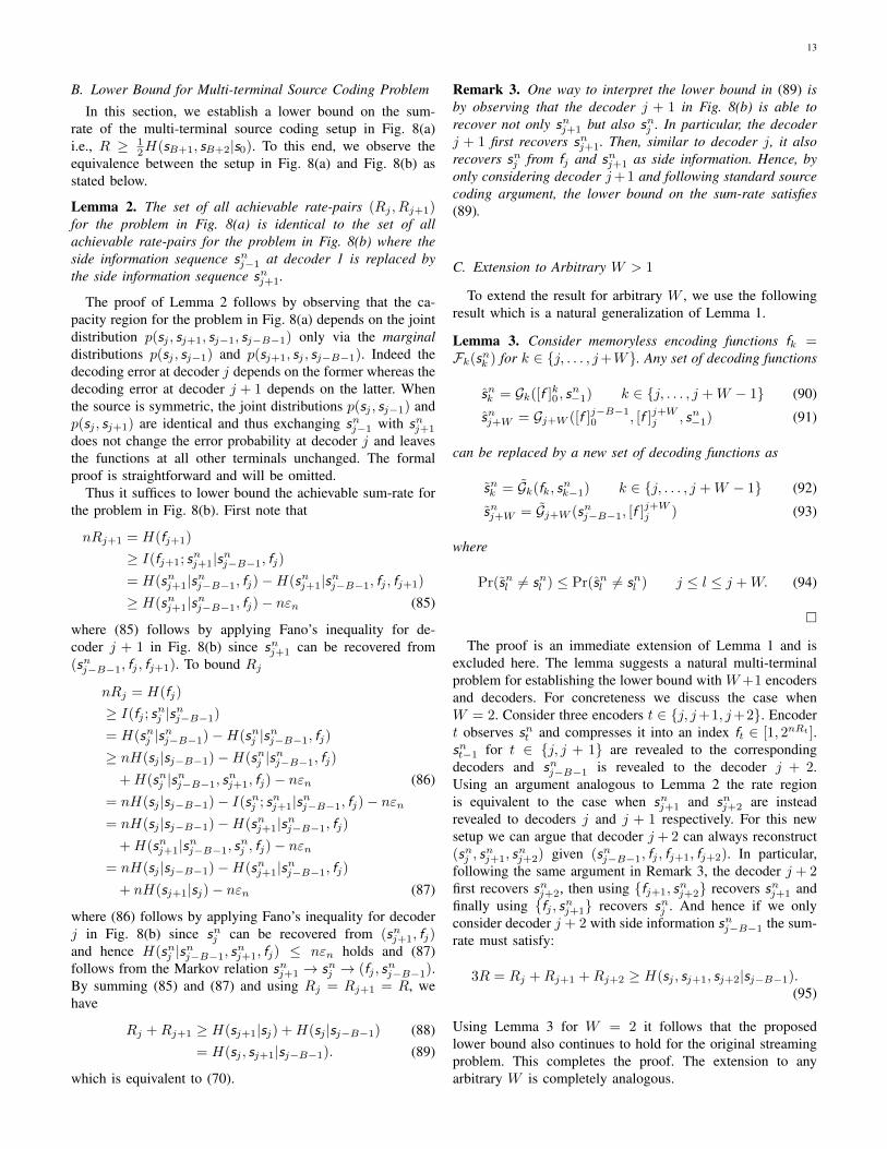
Fig. 8: Connection between the streaming problem and the multi-terminal source coding problem. The setup on the right isidentical to the setup on the left, except with the side information sequence snj−1 replaced with snj+1. However the rate regionfor both problems are identical for symmetric Markov sources.

where (71) follows from the Markov chain property sj−B−1 →sj → sj+1, and the last step in (72) follows from stationarityof the source model.

To establish (70) we make a connection to a multi-terminalsource coding problem in Fig. 8(a). We accomplish this inseveral steps as outlined below.

A. Multi-Terminal Source Coding

Consider the multi-terminal source coding problem withside information illustrated in Fig. 8(a). In this setup there arefour source sequences drawn i.i.d. from a joint distributionp(sj+1, sj , sj−1, sj−B−1). The two source sequences snj andsnj+1 are revealed to the encoders j and j+ 1 respectively andthe two sources snj−1 and snj−B−1 are revealed to the decodersj and j + 1 respectively. The encoders operate independentlyand compress the source sequences to fj and fj+1 at ratesRj and Rj+1 respectively. Decoder j has access to (fj , s

nj−1)

while decoder j + 1 has access to (fj , fj+1, snj−B−1). The two

decoders are required to reconstruct

snj = Gj(fj , snj−1) (73)

snj+1 = Gj+1(fj , fj+1, snj−B−1) (74)

respectively such that Pr(sni 6= sni ) ≤ εn for i = j, j + 1.Note that the multi-terminal source coding setup in Fig. 8(a)

is similar to the setup in Fig. 7, except that the encoders do notcooperate and fi = Fi(sni ), due to the memoryless property.We exploit this property to directly show that a lower boundon the multi-terminal source coding setup in Fig. 8(a) alsoconstitutes a lower bound on the rate of the original streamingproblem.

Lemma 1. For the class of memoryless encoding functions,i.e. fj = Fj(snj ), the decoding functions snj = Gj([f ]j0, s

n−1)

and snj+1 = Gj+1([f ]j−20 , fj , fj+1, s

n−1) can be replaced by the

following decoding functions

snj = Gj(fj , snj−1) (75)

snj+1 = Gj+1(fj , fj+1, snj−2, ) (76)

such that

Pr(snj 6= snj ) ≤ Pr(snj 6= snj ) (77)

Pr(snj+1 6= snj+1) ≤ Pr(snj+1 6= snj+1). (78)

Proof. Assume that the extra side-informations snj−1 is re-vealed to the decoder j. Now define the maximum a posterioriprobability (MAP) decoder as follow.

snj = Gj([f ]j0, sn−1, s

nj−1) , argmax

snj

p(snj |[f ]j0, sn−1, s

nj−1)

(79)

where we dropped the subscript in conditional probabilitydensity for sake of simplicity. It is known that the MAP de-coder is optimal and minimizes the decoding error probability,therefore

Pr(snj 6= snj ) ≤ Pr(snj 6= snj ) (80)

Also note that

snj = Gj([f ]j0, sn−1, s

nj−1) = argmax

snj

p(snj |[f ]j0, sn−1, s

nj−1)

(81)= argmax

snj

p(snj |fj , snj−1) (82)

, Gj(fj , snj−1) (83)

where (82) follows form the following Markov property.([f ]j−1

0 , sn−1

)→ (fj , s

nj−1)→ snj . (84)

It can be shown through similar steps that the decoder definedin (76) exists with the error probability satisfying (78). Thiscompletes the proof.

The conditions in (75) and (76) show that any rate that isachievable in the streaming problem in Fig. 1 is also achievedin the multi-terminal source coding setup in Fig. 8(a). Hencea lower bound to this source network also constitutes a lowerbound to the original problem. In the next section we find alower bound on the rate for the setup in Fig. 8(a).

13

B. Lower Bound for Multi-terminal Source Coding Problem

In this section, we establish a lower bound on the sum-rate of the multi-terminal source coding setup in Fig. 8(a)i.e., R ≥ 1

2H(sB+1, sB+2|s0). To this end, we observe theequivalence between the setup in Fig. 8(a) and Fig. 8(b) asstated below.

Lemma 2. The set of all achievable rate-pairs (Rj , Rj+1)for the problem in Fig. 8(a) is identical to the set of allachievable rate-pairs for the problem in Fig. 8(b) where theside information sequence snj−1 at decoder 1 is replaced bythe side information sequence snj+1.

The proof of Lemma 2 follows by observing that the ca-pacity region for the problem in Fig. 8(a) depends on the jointdistribution p(sj , sj+1, sj−1, sj−B−1) only via the marginaldistributions p(sj , sj−1) and p(sj+1, sj , sj−B−1). Indeed thedecoding error at decoder j depends on the former whereas thedecoding error at decoder j + 1 depends on the latter. Whenthe source is symmetric, the joint distributions p(sj , sj−1) andp(sj , sj+1) are identical and thus exchanging snj−1 with snj+1

does not change the error probability at decoder j and leavesthe functions at all other terminals unchanged. The formalproof is straightforward and will be omitted.

Thus it suffices to lower bound the achievable sum-rate forthe problem in Fig. 8(b). First note that

nRj+1 = H(fj+1)

≥ I(fj+1; snj+1|snj−B−1, fj)

= H(snj+1|snj−B−1, fj)−H(snj+1|snj−B−1, fj , fj+1)

≥ H(snj+1|snj−B−1, fj)− nεn (85)

where (85) follows by applying Fano’s inequality for de-coder j + 1 in Fig. 8(b) since snj+1 can be recovered from(snj−B−1, fj , fj+1). To bound Rj

nRj = H(fj)

≥ I(fj ; snj |snj−B−1)

= H(snj |snj−B−1)−H(snj |snj−B−1, fj)

≥ nH(sj |sj−B−1)−H(snj |snj−B−1, fj)

+H(snj |snj−B−1, snj+1, fj)− nεn (86)

= nH(sj |sj−B−1)− I(snj ; snj+1|snj−B−1, fj)− nεn= nH(sj |sj−B−1)−H(snj+1|snj−B−1, fj)

+H(snj+1|snj−B−1, snj , fj)− nεn

= nH(sj |sj−B−1)−H(snj+1|snj−B−1, fj)

+ nH(sj+1|sj)− nεn (87)

where (86) follows by applying Fano’s inequality for decoderj in Fig. 8(b) since snj can be recovered from (snj+1, fj)and hence H(snj |snj−B−1, s

nj+1, fj) ≤ nεn holds and (87)

follows from the Markov relation snj+1 → snj → (fj , snj−B−1).

By summing (85) and (87) and using Rj = Rj+1 = R, wehave

Rj +Rj+1 ≥ H(sj+1|sj) +H(sj |sj−B−1) (88)= H(sj , sj+1|sj−B−1). (89)

which is equivalent to (70).

Remark 3. One way to interpret the lower bound in (89) isby observing that the decoder j + 1 in Fig. 8(b) is able torecover not only snj+1 but also snj . In particular, the decoderj + 1 first recovers snj+1. Then, similar to decoder j, it alsorecovers snj from fj and snj+1 as side information. Hence, byonly considering decoder j+1 and following standard sourcecoding argument, the lower bound on the sum-rate satisfies(89).

C. Extension to Arbitrary W > 1

To extend the result for arbitrary W , we use the followingresult which is a natural generalization of Lemma 1.

Lemma 3. Consider memoryless encoding functions fk =Fk(snk ) for k ∈ j, . . . , j+W. Any set of decoding functions

snk = Gk([f ]k0 , sn−1) k ∈ j, . . . , j +W − 1 (90)

snj+W = Gj+W ([f ]j−B−10 , [f ]j+Wj , sn−1) (91)

can be replaced by a new set of decoding functions as

snk = Gk(fk, snk−1) k ∈ j, . . . , j +W − 1 (92)

snj+W = Gj+W (snj−B−1, [f ]j+Wj ) (93)

where

Pr(snl 6= snl ) ≤ Pr(snl 6= snl ) j ≤ l ≤ j +W. (94)

The proof is an immediate extension of Lemma 1 and isexcluded here. The lemma suggests a natural multi-terminalproblem for establishing the lower bound with W+1 encodersand decoders. For concreteness we discuss the case whenW = 2. Consider three encoders t ∈ j, j+1, j+2. Encodert observes snt and compresses it into an index ft ∈ [1, 2nRt ].snt−1 for t ∈ j, j + 1 are revealed to the correspondingdecoders and snj−B−1 is revealed to the decoder j + 2.Using an argument analogous to Lemma 2 the rate regionis equivalent to the case when snj+1 and snj+2 are insteadrevealed to decoders j and j + 1 respectively. For this newsetup we can argue that decoder j + 2 can always reconstruct(snj , s

nj+1, s

nj+2) given (snj−B−1, fj , fj+1, fj+2). In particular,

following the same argument in Remark 3, the decoder j + 2first recovers snj+2, then using fj+1, s

nj+2 recovers snj+1 and

finally using fj , snj+1 recovers snj . And hence if we onlyconsider decoder j + 2 with side information snj−B−1 the sum-rate must satisfy:

3R = Rj +Rj+1 +Rj+2 ≥ H(sj , sj+1, sj+2|sj−B−1).(95)

Using Lemma 3 for W = 2 it follows that the proposedlower bound also continues to hold for the original streamingproblem. This completes the proof. The extension to anyarbitrary W is completely analogous.

14

VII. LOSSY RATE-RECOVERY FOR GAUSS-MARKOVSOURCES

We establish lower and upper bounds on the lossy rate-recovery function of Gauss-Markov sources when an imme-diate recovery following the burst erasure is required i.e.,W = 0. For the single burst erasure case, the proof of thelower bound in Prop. 1 is presented in Section VII-A whereasthe proof of the upper bound in Prop. 2 is presented inSection VII-B. The proof of Prop. 3 for the multiple burst era-sures case is presented in Section VII-C. Finally the proof ofCorollary 3, which establishes the lossy rate-recovery functionin the high resolution regime is presented in Section VII-D.

A. Lower Bound: Single Burst Erasure

Consider any rate R code that satisfies an average distortionof D as stated in (5). For each i ≥ 0 we have

nR ≥ H(fi)

≥ H(fi|[f ]i−B−10 , sn−1) (96)

= I(sni ; fi|[f ]i−B−10 , sn−1) +H(fi|sni , [f ]i−B−1

0 , sn−1)

≥ h(sni |[f ]i−B−10 , sn−1)− h(sni |fi, [f ]i−B−1

0 , sn−1) (97)

where (96) follows from the fact that conditioning reduces theentropy.

We now present an upper bound for the second term anda lower bound for the first term in (97). We first establish anupper bound for the second term in (97). Suppose that the bursterasure occurs in the interval [i−B, i− 1]. The reconstructionsequence sni must be a function of (fi, [f ]i−B−1

0 , sn−1). Thuswe have

h(sni |[f ]i−B−10 , fi, s

n−1) = h(sni − sni | [f ]i−B−1

0 , fi, sn−1)

≤ h(sni − sni )

≤ n

2log(2πeD), (98)

where the last step uses the fact that the expected averagedistortion between sni and sni is no greater than D, and appliesstandard arguments [29, Ch. 13].

To lower bound the first term in (97), we successively usethe Gauss-Markov relation (11) to express:

si = ρ(B+1)si−B−1 + n (99)

for each i ≥ B and n ∼ N (0, 1− ρ2(B+1)) is independent ofsi−B−1. Using the Entropy Power Inequality [29] we have

22nh(sni |[f ]i−B−1

0 ,sn−1) ≥

22nh(ρB+1sni−B−1|[f ]i−B−1

0 ,sn−1) + 22nh(nn) (100)

This further reduces to

h(sni | [f ]i−B−10 , sn−1) ≥

n

2log(ρ2(B+1)2

2nh(sni−B−1|[f ]i−B−1

0 ,sn−1)+2πe(1−ρ2(B+1))).

(101)

It remains to lower bound the entropy term in the right handside of (101). We show the following in Appendix B.

Lemma 4. For any k ≥ 0

22nh(snk |[f ]k0 ,s

n−1) ≥ 2πe(1− ρ2)

22R − ρ2

(1−

(ρ2

22R

)k)(102)

Upon substituting, (102), (101), and (98) into (97) we obtainthat for each i ≥ B + 1

R ≥ 1

2log

[ρ2(B+1)(1− ρ2)

D(22R − ρ2)

(1−

(ρ2

22R

)i−B−1)

+1− ρ2(B+1)

D

]. (103)

Selecting the largest value of i, i.e. L, yields the tightestlower bound. As mentioned earlier, we are interested in infinitehorizon when L → ∞, which yields the tightest lower bound,we have

R ≥ 1

2log

(ρ2(B+1)(1− ρ2)

D(22R − ρ2)+

1− ρ2(B+1)

D

)(104)

Rearranging (104) we have that

D24R − (Dρ2 + 1− ρ2(B+1))22R + ρ2(1− ρ2B) ≥ 0(105)

Since (105) is a quadratic equation in 22R, it can be easilysolved. Keeping the root that yields R > 0 results in the lowerbound in (12) in Prop. 1. This completes the proof.

Remark 4. Upon examining the proof of the lower bound ofProp. 1, we note that it applies to any source process thatsatisfies (11) and where the additive noise is i.i.d. N (0, 1 −ρ2). We do not use the fact that the source process is itself aGaussian process.

B. Coding Scheme: Single Burst Erasure

The achievable rate is based on quantization and binning.For each i ≥ 0, we consider the test channel

ui = si + zi, (106)

where zi ∼ N (0, σ2z) is independent Gaussian noise. At time

i we sample a total of 2n(I(ui;si)+ε) codeword sequences i.i.d.from N (0, 1 + σ2

z). The codebook at each time is partitionedinto 2nR bins. The encoder finds the codeword sequence unitypical with the source sequence sni and transmits the bin indexfi assigned to uni .

The decoder, upon receiving fi attempts to decode uni attime i, using all the previously recovered codewords unj :0 ≤ j ≤ i − 1, gj 6= ? and the source sequence sn−1 as sideinformation. The reconstruction sequence sni is the minimummean square error (MMSE) estimate of sni given uni and thepast sequences. The coding scheme presented here is based onbinning, similar to lossless case discussed in Section V-C. Themain difference in the analysis is that, unlike the lossless case,neither the recovered sequences uni nor reconstructed sourcesequences sni inherit the Markov property of the originalsource sequences sni . Therefore, unlike the lossless case, the

15

Lemma 5:Connection to Gaussian Many-help-one

Source Coding Problem.

Lemma 6:Worst-case Characterization of Burst

Erasure and Steady State Analysis.

Lemma 7 and Section VII-B2:Rate Evaluation

Fig. 9: Flowchart summarizing the proof steps of Prop. 2.

B′

s−1 X X X X X X X X X? ? ? ? ?

1 t−B′−k t−k−1 t

Fig. 10: Schematic of single burst erasure channel model. Thechannel inputs in the interval [t−B′−k, t−k−1] is erased forsome 0 ≤ B′ ≤ B and k ∈ [0, t− B′]. The rest are availableat the decoder, as shown by check mark in the figure.

decoder does not reset following a burst erasure, once theerror propagation is completed. Since the effect of a bursterasure persists throughout, the analysis of achievable rate issignificantly more involved.

Fig. 9 summarizes the main steps in proving Prop. 2. Inparticular, in Lemma 5, we first derive necessary parametricrate constraints associated with every possible erasure pattern.Second, through the Lemma 6, we characterize the the worst-case erasure pattern that dominates the rate and distortionconstraints. Finally in Lemma 7 and Section VII-B2, weevaluate the achievable rate to complete the proof of Prop. 2.

1) Analysis of Achievable Rate: Given a collection ofrandom variables V , we let the MMSE estimate of si bedenoted by si(V), and its associated estimation error is denotedby σ2

i (V), i.e.,

si(V)= E [si | V] (107)

σ2i (V)= E[(si − si(V))

2]. (108)

We begin with a parametric characterization of the achiev-able rate.

Lemma 5. A rate-distortion pair (R,D) is achievable, if forevery t ≥ 0, B′ ∈ [0, B] and k ∈ [0, t−B′] we have

R ≥ λt(k,B′) , I(st; ut | [u]t−B′−k−1

0 , [u]t−1t−k, s−1), (109)

and the test-channel (106) satisfies

γt(k,B′) , E

[(st − st([u]t−B

′−k−10 , [u]tt−k, s−1)

)2]

= σ2t ([u]t−B

′−k−10 , [u]tt−k, s−1) ≤ D. (110)

where σ2t (·) and st(·) are defined in (108) and (107) respec-

tively.

Proof. Consider the decoder at any time t ≥ 0 outside theerror propagation window. Assume that a single burst erasureof length B′ ∈ [0, B] spans the interval [t−B′− k, t− k− 1]for some k ∈ [0, t−B′] i.e.,

gj =

?, j ∈ t−B′ − k, . . . , t− k − 1fj , else.

(111)

The schematic of the erasure channel is illustrated in Fig. 10.Notice that k = 0 represents the case of the most recentburst erasure spanning the interval [t − B′ − 1, t − 1]. Thedecoder is interested in first successfully recovering unt andthen reconstructing snt within distortion D by performingMMSE estimation of snt from all the previously recoveredsequences uni where i ≤ t and gi 6= ?. The decoder succeedswith high probability if the rate constraint satisfies (109) (seee.g., [30]) and the distortion constraint satisfies (110). If theseconstraints hold for all the possible triplets (t, B′, k), thedecoder is guaranteed to succeed in reproducing any sourcesequence within desired distortion D.

Finally in the streaming setup, we can follow the argumentsimilar to that in Section V-C to argue that the decodersucceeds in the entire horizon of L provided we select thesource length n to be sufficiently large. The formal proof isomitted here.

As a result of Lemma 5, in order to compute the achievablerate, we need to characterize the worst case values of (t, k, B′)that simultaneously maximize λt(k,B) and γt(k,B). Wepresent such a characterization next.

Lemma 6. The functions λt(k,B) and γt(k,B) satisfy thefollowing properties:

1) For all t ≥ B′ and k ∈ [0, t−B′], λt(k,B′) ≤ λt(0, B′)and γt(k,B

′) ≤ γt(0, B′), i.e. the worst-case erasure

pattern contains the burst erasure in the interval [t −B, t− 1].

2) For all t ≥ B and 0 ≤ B′ ≤ B, λt(0, B′) ≤ λt(0, B)and γt(0, B

′) ≤ γt(0, B), i.e. the worse-case erasurepattern includes maximum burst length.

3) For a fixed B, the functions λt(0, B) and γt(0, B) areboth increasing with respect to t, for t ≥ B, i.e. theworse-case erasure pattern happens in steady state (i.e.,t→∞) of the system.

4) For all t < B, 0 ≤ B′ ≤ t and k ∈ [0, t − B′],λt(k,B

′) ≤ λB(0, B) and γt(k,B′) ≤ γB(0, B) i.e.,

the burst erasure spanning [0, B−1] dominates all bursterasures that terminate before time B − 1.

Proof. Before establishing the proof, we state two inequalitieswhich are established in Appendix C. For each k ∈ [1 : t−B′]

16

s−1 s0 st−B′−k−1 st−B′−k st−k st−k+1 st−1 st

u0 ut−B′−k−1 ut−B′−k ut−k ut−k+1 ut−1 ut

Fig. 11: Replacing ut−B′−k by ut−k improves the estimate ofst and ut.

we have that:

h(ut|[u]t−B′−k−1

0 , [u]t−1t−k, s−1)

≤ h(ut|[u]t−B′−k

0 , [u]t−1t−k+1, s−1), (112)

h(st|[u]t−B′−k−1

0 , [u]tt−k, s−1)

≤ h(st|[u]t−B′−k

0 , [u]tt−k+1, s−1). (113)

The above inequalities state that the conditional differentialentropy of ut and st is reduced if the variable ut−B′−k is re-placed by ut−k in the conditioning and the remaining variablesremain unchanged. Fig. 11 provides a schematic interpretationof the above inequalities. The proof in Appendix C exploitsthe specific structure of the Gaussian test channel (106) andGaussian sources to establish these inequalities.

In the remainder of the proof, we establish each of the fourproperties separately.

1) We show that both λt(k,B′) and γt(k,B′) are decreasingfunctions of k for k ∈ [1 : t−B′].

λt(k,B′) = I(st; ut|[u]t−B

′−k−10 , [u]t−1

t−k, s−1)

= h(ut|[u]t−B′−k−1

0 , [u]t−1t−k, s−1)− h(ut|st)

≤ h(ut|[u]t−B′−k

0 , [u]t−1t−k+1, s−1)− h(ut|st)

(114)

= I(st; ut|[u]t−B′−k

0 , [u]t−1t−k+1, s−1)

= λt(k − 1, B′) (115)

where (114) follows from using (112). In a similar fashionsince

γt(k,B′) = σ2

t

([u]t−B

′−k0 , [u]tt−k+1, s−1

)is the MMSE estimation error of st given(

[u]t−B′−k

0 , [u]tt−k+1, s−1

), we have

1

2log (2πe · γt(k,B′)) = h(st|[u]t−B

′−k−10 , [u]tt−k, s−1)

≤ h(st|[u]t−B′−k

0 , [u]tt−k+1, s−1)(116)

=1

2log (2πe · γt(k − 1, B′)) (117)

where (116) follows from using (113). Since f(x) =12 log(2πex) is a monotonically increasing function it followsthat γt(k,B′) ≤ γt(k − 1, B′). By recursively applying (115)and (117) until k = 1, the proof of property (1) is complete.

2) We next show that the worst case erasure pattern alsohas the longest burst. This follows intuitively since the decoder

can just ignore some of the symbols received over the channel.Thus any rate achieved with the longest burst is also achievedfor the shorter burst. The formal justification is as follows. Forany B′ ≤ B we have,

λt(0, B′) = I(st; ut|[u]t−B

′−10 , s−1)

= h(ut|[u]t−B′−1

0 , s−1)− h(ut|st) (118)

= h(ut|[u]t−B−10 , [u]t−B

′−1t−B , s−1)− h(ut|st)

≤ h(ut|[u]t−B−10 , s−1)− h(ut|st) (119)

= I(st; ut|[u]t−B−10 , s−1) (120)

= λt(0, B) (121)

where (118) and (120) follows from the Markov chainproperty

ut → st → [u]t−j−10 , s−1, j ∈ B,B′ (122)

and (119) follows from the fact that conditioning reducesdifferential entropy. In a similar fashion the inequalityγt(0, B

′) ≤ γt(0, B) follows from the fact that the estimationerror can only be reduced by having more observations.

3) We show that both λt(0, B) and γt(0, B) are increasingfunctions with respect to t. Intuitively as t increases the effectof having s−1 at the decoder vanishes and hence the requiredrate increases. Consider

λt+1(0, B) = I(st+1; ut+1|[u]t−B0 , s−1)

= h(ut+1|[u]t−B0 , s−1)− h(ut+1|st+1)

= h(ut+1|[u]t−B0 , s−1)− h(ut|st) (123)

≥ h(ut+1|[u]t−B0 , s−1, s0)− h(ut|st) (124)

= h(ut+1|[u]t−B1 , s0)− h(ut|st) (125)

= h(ut|[u]t−B−10 , s−1)− h(ut|st) (126)

= I(st; ut|[u]t−B−10 , s−1)

= λt(0, B) (127)

where (123) and (126) follow from time-invariant property ofthe source model and the test channel, (124) follows from thefact that conditioning reduces differential entropy and (125)uses the following Markov chain property

u0, s−1 → [u]t−B1 , s0 → ut+1. (128)

Similarly,

1

2log (2πe · γt+1(0, B)) = h(st+1|[u]t−B0 , ut+1, s−1)

≥ h(st+1|[u]t−B0 , ut+1, s0, s−1)

= h(st+1|[u]t−B1 , ut+1, s0) (129)

= h(st|[u]t−B−10 , ut, s−1)

=1

2log (2πe · γt(0, B)) (130)

where (129) follows from the following Markov chain property

u0, s−1 → [u]t−B1 , ut+1, s0 → st+1. (131)

Since (127) and (130) hold for every t ≥ B the proof ofproperty (3) is complete.

17

4) Note that for t < B we have 0 ≤ B′ ≤ t and thus wecan write

λt(k,B′) ≤ λt(0, B′) (132)≤ λt(0, t) (133)= h(ut|s−1)− h(ut|st)= h(ut|s−1)− h(uB |sB)

= h(uB |sB−t−1)− h(uB |sB)

≤ h(uB |s−1)− h(uB |sB) (134)= λB(0, B) (135)

where (132) follows from part 1 of the lemma, (133) is basedon the fact that the worse-case erasure pattern contains mostpossible erasures and follows from the similar steps used inderiving (121) and using the fact that if t < B, the bursterasure length is at most t. Eq. (134) follows from the factthat whenever t < B the relation s−1 → sB−t−1 → uB holdssince t < B is assumed. In a similar fashion we can show thatγt(k,B

′) ≤ γB(0, B).This completes the proof of lemma 6.

Following the four parts of Lemma 6, it follows that theworst-case erasure pattern happens at steady state i.e. t→∞when there is a burst of length B which spans [t−B, t− 1].According to this and Lemma 5, any pair (R,D) is achievableif

R ≥ limt→∞

λt(0, B) (136)

D ≥ limt→∞

γt(0, B) (137)

Lemma 7. Consider ui = si + zi and suppose the noisevariance σ2

z satisfies

Γ(B, σ2z) , lim

t→∞E[(st − st([u]t−B−1

0 , ut))2]

(138)

= limt→∞

σ2t

([u]t−B−1

0 , ut)≤ D. (139)

The following rate is achievable:

R = Λ(B, σ2z) , lim

t→∞I(st; ut|[u]t−B−1

0 ). (140)

Proof. It suffices to show that any test channel satisfying (139)also implies (137) and any rate satisfying (140) implies (136).These relations can be established in a straightforward manneras shown below.

R = Λ(B, σ2z) = lim

t→∞I(st; ut|[u]t−B−1

0 )

= limt→∞

(h(ut|[u]t−B−1

0 )− h(ut|st))

(141)

≥ limt→∞

(h(ut|[u]t−B−1

0 , s−1)− h(ut|st))

(142)= limt→∞

λt(0, B) (143)

and

D ≥ Γ(B, σ2z) = lim

t→∞E[(st − st([u]t−B−1

0 , ut))2]

(144)

≥ limt→∞

E[(st − st([u]t−B−1

0 , ut, s−1))2](145)

= limt→∞

γt(0, B) (146)

We conclude that Γ(B, σ2z) = D, the rate R+

GM-SE(B,D) =Λ(B, σ2

z) is achievable.2) Numerical Evaluation: We derive an expression for

numerically evaluating the noise variance σ2z in (106) and also

establish (13) and (16).To this end it is helpful to consider the following single-

variable discrete-time Kalman filter for i ∈ [0, t−B − 1],

si = ρsi−1 + ni, ni ∼ N(0, 1− ρ2) (147)

ui = si + zi, zi ∼ N(0, σ2z). (148)

Note that si can be viewed as the state of the system updatedaccording a Gauss-Markov model and ui as the output of thesystem at each time i, which is a noisy version of the state si.Consider the system in steady state i.e. t → ∞. The MMSEestimation error of st−B given all the previous outputs up totime t − B − 1 i.e. [u]t−B−1

0 is expressed as (see, e.g., [31,Example V.B.2]):

Σ(σ2z) , lim

t→∞σ2t−B([u]t−B−1

0 ) (149)

=1

2

√(1− σ2

z)2(1− ρ2)2 + 4σ2z(1− ρ2) +

1− ρ2

2(1− σ2

z)

(150)

Also using the orthogonality principle for MMSE estimationwe have

[u]t−B−10 → st−B([u]t−B−1

0 )→ st−B → st (151)

Thus we can express

st−B = st−B([u]t−B−10 ) + e (152)

where the noise e ∼ N (0,Σ(σ2z

)) is independent of the

observation set [u]t−B−10 . Equivalently we can express (see

e.g. [32])

st−B([u]t−B−10 ) = αst−B + e (153)

where

α , 1− Σ(σ2z

)(154)

and e ∼ N(0,Σ

(σ2z

) (1− Σ

(σ2z

)))is independent of st−B .

Thus we have

Λ(B, σ2z) = lim

t→∞I(st; ut|[u]t−B−1

0 )

= limt→∞

I(st; ut|st−B([u]t−B−10 ))

= limt→∞

I(st; ut|αst−B + e)

= limt→∞

I(st; ut|st−B + e)

= I(st; ut|st−B) (155)

18

where we have used (153) ande ∼ N (0,Σ

(σ2z

)/(1− Σ

(σ2z

))). This establishes (13)

in Prop. 2. In a similar manner,

Γ(B, σ2z) = lim

t→∞σ2t ([u]t−B−1

0 , ut)

= limt→∞

σ2t (st−B([u]t−B−1

0 ), ut)

= limt→∞

σ2t (αst−B + e, , ut)

= limt→∞

σ2t (st−B + e, ut)

= σ2t (st−B , ut) (156)

which establishes (16). Furthermore since

st = ρBst−B + n (157)

where n ∼ N (0, 1− ρ2B),

Γ(B, σ2z) = σ2

t (st−B , ut) (158)

=

[1

σ2z

+1

1− ρ2B (1− Σ(σ2z))

]−1

(159)

where (159) follows from the application of MMSE estimatorand using (157), (152) and the definition of the test channel in(106). Thus the noise σ2

z in the test channel (106) is obtainedby setting

Γ(B, σ2z) = D. (160)

This completes the proof of Prop. 2.

Remark 5. When W > 0, the generalization of Lemma 6appears to involve a rate-region corresponding to the Berger-Tung inner bound [33] and the analysis is considerably moreinvolved. Furthermore hybrid schemes involving predictivecoding and binning may lead to an improved performanceover the binning-only scheme. Thus the scope of this problemis well beyond the results in this paper.

C. Coding Scheme: Multiple Burst Erasures with Guard In-tervals

We study the achievable rate using the quantize and binningscheme with test channel (106) when the channel introducesmultiple burst erasures each of length no greater than Band with a guard interval of at-least L symbols separatingconsecutive burst erasures. While the coding scheme is thesame as the single burst erasure channel model and is basedon quantize and binning and MMSE estimation at the decoder,characterizing the worst case erasure pattern of the channel ismain challenge and requires some additional steps.

1) Analysis of Achievable Rate: We introduce the followingnotation in our analysis. Let Ωt denote the set of time indicesup to time t− 1 when the channel packets are not erased i.e.,

Ωt = i : 0 ≤ i ≤ t− 1, gi 6= ?, (161)

and let us define

sΩ = si : i ∈ Ω, (162)uΩ = ui : i ∈ Ω. (163)

B BL L

sts−1

? ? ? ? ?X X X X X X X X X X X X X X

(0) (1) (2) (3) (4) (5) (6) (8) (9) (10) (13)(14)(15)

(a) Ω?18(13)=0, 1, 2, 3, 4, 5, 6, 8, 9, 10, 13, 14, 15B B B BL L L

sts−1

? ? ? ? ? ? ? ?X X X X X X X X X X X

(0) (3) (4) (5) (8) (9) (10) (13)(14)(15)

(b) Ω?18 =0, 3, 4, 5, 8, 9, 10, 13, 14, 15

Fig. 12: Schematic of the erasure patterns in Lemma 9 fort = 18, L = 3 and B = 2. Fig. 12a illustrates, Ω?t (θ) in part 1of Lemma 9. The non-erased symbols are denoted by check-marks. Fig. 12b illustrates Ω?t as stated in part 2 of Lemma 9.

Given the erasure sequence Ωt, and given gt = ft, thedecoder can reconstruct unt provided that the test channel isselected such that the rate satisfies (see e.g., [30])

R ≥ λt(Ωt) , I(st; ut|uΩt, s−1). (164)

and the distortion constraint satisfies

γt(Ωt) , E[(st − st(uΩt

, ut, s−1))2]

= σ2t (uΩt , ut, s−1) ≤ D (165)

for each t ≥ 0 and each feasible set Ωt. Thus we areagain required to characterize the Ωt for each value of tcorresponding to the worst-case erasure pattern. The followingtwo lemmas are useful towards this end.

Lemma 8. Consider the two sets A,B ⊆ N each of sizer as A = a1, a2, · · · , ar, B = b1, b2, · · · , br such that1 ≤ a1 < a2 < · · · < ar and 1 ≤ b1 < b2 < · · · < br andfor any i ∈ 1, . . . , r, ai ≤ bi. Then the test channel (106)satisfies the following:

h(st|uA, s−1) ≥ h(st|uB , s−1), ∀t ≥ br (166)h(ut|uA, s−1) ≥ h(ut|uB , s−1), ∀t > br. (167)

The proof of Lemma 8 is available in Appendix D.

Lemma 9. Assume that at time t, gt = ft and let Ωt be asdefined in (161) .

1) Among all feasible sets Ωt of size |Ωt| = θ, λt(Ωt)and γt(Ωt) are maximized by a set Ω?t (θ) where all theerasures happen in the closest possible locations to timet.

2) For each fixed t, both λt(Ω?t (θ)) and γt(Ω?t (θ)) are max-imized by the minimum possible value of θ. Equivalently,the maximizing set, denoted by Ω?t , corresponds to theerasure pattern with maximum number of erasures.

3) Both λt(Ω?t ) and γt(Ω

?t ) are increasing functions with

respect to t.

The proof of Lemma 9 is presented in Appendix E. Wepresent an example in Fig. 12 to illustrate Lemma 9. We

19

assume t = 18. The total number of possible erasures upto time t = 18 is restricted to be 5, or equivalently thenumber of non-erased packets is θ = 13 in Fig 12a. The setΩ?18(13) indicates the set of non-erased indices associated withthe worst case erasure pattern. Based on part 2 of Lemma 9,Fig. 12b shows the worst case erasure pattern for time t = 18,which includes the maximum possible erasures.

Following the three steps in Lemma 9 a rate-distortion pair(R,D) is achievable if

R ≥ limt→∞

λt(Ω?t ) (168)

D ≥ limt→∞

γt(Ω?t ) (169)

Lemma 10. Any test channel noise σ2z satisfying (19) and (20)

in Prop. 3, i.e.

R ≥ I(st; ut|st−L−B , [u]t−B−1t−L−B+1) (170)

D ≥ σ2t (st−L−B , [u]t−B−1

t−L−B+1, ut) (171)

where st−L−B = st−L−B + e, where e ∼ N (0, D/(1−D)),also satisfies (168) and (169).

Proof. See Appendix F.

This completes the proof of Prop 3.2) Numerical Evaluation: We derive the expression for nu-

merically evaluating σ2z . To this end, first note that the estima-

tion error of estimating st−B−1 from st−L−B , [u]t−B−1t−L−B+1

can be computed as follows.

η(σ2z) , σ2

t−B−1(st−L−B , [u]t−B−1t−L−B+1)

= E[s2t−B−1

]− E [st−B−1U]

(E[UTU

])−1E[st−B−1U

T]

(172)

= 1−A1(A2)−1AT1 (173)

where we define

U ,[ut−B−1 ut−B−2 . . . ut−L−B+1 st−L−B

]and (.)T denotes the transpose operation. Also note that A1

and A2 can be computed as follows.

A1 = (1, ρ, ρ2, · · · , ρL−1) (174)

A2 =

1 + σ2

z ρ · · · ρL−2 ρL−1

ρ 1 + σ2z · · · ρL−3 ρL−2

......

. . ....

...ρL−2 ρL−3 · · · 1 + σ2

z ρρL−1 ρL−2 · · · ρ 1 + D

1−D

(175)

According to (171) we can write

D = σ2t (st−L−B , [u]t−B−1

t−L−B+1, ut) (176)

= σ2t

(st−B−1(st−L−B , [u]t−B−1

t−L−B+1), ut)

=

[1

σ2z

+1

1− ρ2(B+1)(1− η(σ2z))

]−1

(177)

Therefore by solving (177) the expression for σ2z can be

obtained. Finally the achievable rate is computed as:

R+GM-ME(L,B,D) = I(st; ut|st−L−B , [u]t−B−1

t−L−B+1)

= h(st|st−L−B , [u]t−B−1t−L−B+1)− h(st|st−L−B , [u]t−B−1

t−L−B+1, ut)

= h(st|st−B−1(st−L−B , [u]t−B−1

t−L−B+1))− 1

2log(2πeD)

=1

2log(

2πe(

1− ρ2(B+1)(1− η(σ2z))))− 1

2log(2πeD)

=1

2log

(1− ρ2(B+1)(1− η(σ2

z))

D

). (178)

D. High Resolution Regime

We investigate the behavior of the lossy rate-recoveryfunctions for Gauss-Markov sources for single and multi-ple burst erasure channel models, i.e. RGM-SE(B,D) andRGM-ME(L,B,D), in the high resolution regime and establishCorollary 3. The following inequalities can be readily verified.

R−GM-SE(B,D) ≤ RGM-SE(B,D) ≤RGM-ME(L,B,D) ≤ R+

GM-ME(L,B,D) (179)

The first and the last inequalities in (179) are by definition andthe second inequality follows from the fact that the rate achiev-able for multiple erasure model is also achievable for singleburst erasure as the decoder can simply ignore the availablecodewords in reconstructing the source sequences. Accordingto (179), it suffices to characterize the high resolution limit ofR−GM-SE(B,D) and R+

GM-ME(L,B,D) in Prop. 1 and Prop. 3respectively.

For the lower bound note that as D → 0 the expression for∆ in (12) satisfies

∆ , (Dρ2+1−ρ2(B+1))2−4Dρ2(1−ρ2B)→ (1−ρ2(B+1))2.

Upon direct substitution in (12) we have that

limD→0

R−GM-SE(B,D)− 1

2log

(1− ρ2(B+1)

D

)= 0, (180)

as required.To establish the upper bound note that according to Prop. 3

we can write

R+GM-ME(L,B,D)

= I(st; ut|st−L−B , [u]t−B−1t−L−B+1)

= h(st|st−L−B , [u]t−B−1t−L−B+1)− h(st|st−L−B , [u]t−B−1

t−L−B+1, ut)

= h(st|st−L−B , [u]t−B−1t−L−B+1)− 1

2log(2πeD) (181)

where the last term follows from the definition of st−L−B inProp. 3. Also we have

h(st|st−B−1) ≤ h(st|st−L−B , [u]t−B−1t−L−B+1) ≤ h(st|ut−B−1)

(182)

where the left hand side inequality in (182) follows from thefollowing Markov property,

st−L−B , [u]t−B−1t−L−B+1 → st−B−1 → st (183)

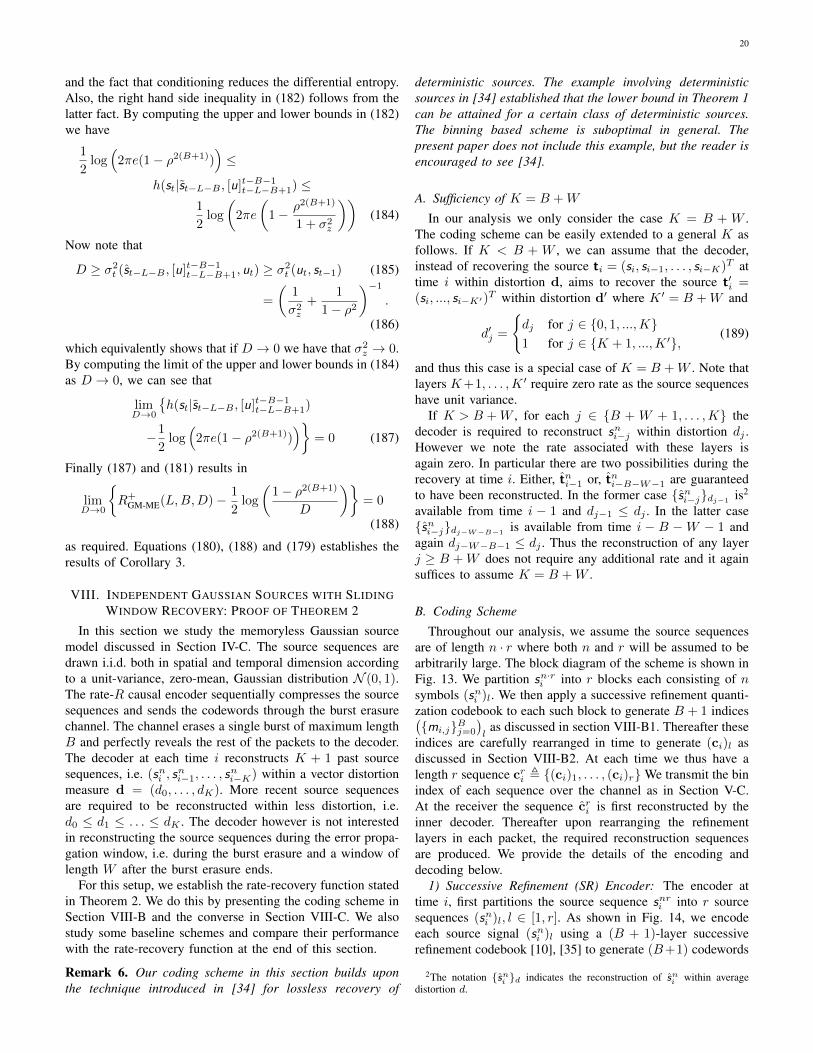
20

and the fact that conditioning reduces the differential entropy.Also, the right hand side inequality in (182) follows from thelatter fact. By computing the upper and lower bounds in (182)we have

1

2log(

2πe(1− ρ2(B+1)))≤

h(st|st−L−B , [u]t−B−1t−L−B+1) ≤

1

2log

(2πe

(1− ρ2(B+1)

1 + σ2z

))(184)

Now note that

D ≥ σ2t (st−L−B , [u]t−B−1

t−L−B+1, ut) ≥ σ2t (ut, st−1) (185)

=

(1

σ2z

+1

1− ρ2

)−1

.

(186)

which equivalently shows that if D → 0 we have that σ2z → 0.

By computing the limit of the upper and lower bounds in (184)as D → 0, we can see that

limD→0

h(st|st−L−B , [u]t−B−1

t−L−B+1)

−1

2log(

2πe(1− ρ2(B+1)))

= 0 (187)

Finally (187) and (181) results in

limD→0

R+

GM-ME(L,B,D)− 1

2log

(1− ρ2(B+1)

D

)= 0

(188)

as required. Equations (180), (188) and (179) establishes theresults of Corollary 3.

VIII. INDEPENDENT GAUSSIAN SOURCES WITH SLIDINGWINDOW RECOVERY: PROOF OF THEOREM 2

In this section we study the memoryless Gaussian sourcemodel discussed in Section IV-C. The source sequences aredrawn i.i.d. both in spatial and temporal dimension accordingto a unit-variance, zero-mean, Gaussian distribution N (0, 1).The rate-R causal encoder sequentially compresses the sourcesequences and sends the codewords through the burst erasurechannel. The channel erases a single burst of maximum lengthB and perfectly reveals the rest of the packets to the decoder.The decoder at each time i reconstructs K + 1 past sourcesequences, i.e. (sni , s

ni−1, . . . , s

ni−K) within a vector distortion

measure d = (d0, . . . , dK). More recent source sequencesare required to be reconstructed within less distortion, i.e.d0 ≤ d1 ≤ . . . ≤ dK . The decoder however is not interestedin reconstructing the source sequences during the error propa-gation window, i.e. during the burst erasure and a window oflength W after the burst erasure ends.

For this setup, we establish the rate-recovery function statedin Theorem 2. We do this by presenting the coding scheme inSection VIII-B and the converse in Section VIII-C. We alsostudy some baseline schemes and compare their performancewith the rate-recovery function at the end of this section.

Remark 6. Our coding scheme in this section builds uponthe technique introduced in [34] for lossless recovery of

deterministic sources. The example involving deterministicsources in [34] established that the lower bound in Theorem 1can be attained for a certain class of deterministic sources.The binning based scheme is suboptimal in general. Thepresent paper does not include this example, but the reader isencouraged to see [34].

A. Sufficiency of K = B +W

In our analysis we only consider the case K = B + W .The coding scheme can be easily extended to a general K asfollows. If K < B + W , we can assume that the decoder,instead of recovering the source ti = (si, si−1, . . . , si−K)T attime i within distortion d, aims to recover the source t′i =(si, ..., si−K′)

T within distortion d′ where K ′ = B +W and

d′j =

dj for j ∈ 0, 1, ...,K1 for j ∈ K + 1, ...,K ′,

(189)

and thus this case is a special case of K = B +W . Note thatlayers K+1, . . . ,K ′ require zero rate as the source sequenceshave unit variance.

If K > B +W , for each j ∈ B + W + 1, . . . ,K thedecoder is required to reconstruct sni−j within distortion dj .However we note the rate associated with these layers isagain zero. In particular there are two possibilities during therecovery at time i. Either, tni−1 or, tni−B−W−1 are guaranteedto have been reconstructed. In the former case sni−jdj−1

is2

available from time i − 1 and dj−1 ≤ dj . In the latter casesni−jdj−W−B−1

is available from time i − B −W − 1 andagain dj−W−B−1 ≤ dj . Thus the reconstruction of any layerj ≥ B +W does not require any additional rate and it againsuffices to assume K = B +W .

B. Coding Scheme

Throughout our analysis, we assume the source sequencesare of length n · r where both n and r will be assumed to bearbitrarily large. The block diagram of the scheme is shown inFig. 13. We partition sn·ri into r blocks each consisting of nsymbols (sni )l. We then apply a successive refinement quanti-zation codebook to each such block to generate B + 1 indices(mi,jBj=0

)l

as discussed in section VIII-B1. Thereafter theseindices are carefully rearranged in time to generate (ci)l asdiscussed in Section VIII-B2. At each time we thus have alength r sequence cri , (ci)1, . . . , (ci)rWe transmit the binindex of each sequence over the channel as in Section V-C.At the receiver the sequence cri is first reconstructed by theinner decoder. Thereafter upon rearranging the refinementlayers in each packet, the required reconstruction sequencesare produced. We provide the details of the encoding anddecoding below.

1) Successive Refinement (SR) Encoder: The encoder attime i, first partitions the source sequence snri into r sourcesequences (sni )l, l ∈ [1, r]. As shown in Fig. 14, we encodeeach source signal (sni )l using a (B + 1)-layer successiverefinement codebook [10], [35] to generate (B+1) codewords

2The notation sni d indicates the reconstruction of sni within averagedistortion d.

21

snri

snri

SourcePartitioning

Block

Bin IndexAssignment

fi ∈ [0, 2nrR]

JointTypicalityDecoder

crj ,i−W≤j≤i

BurstErasureChannel

SourceReproduction

Block

SR Code1

LR Block1

(sni )1 (ci)1(mi,jBj=0)1

SR Code2

LR Block2

(sni )2 (ci)2(mi,jBj=0)2

SR Coder−1

LR Blockr−1

(sni )r−1 (ci)r−1(mi,jBj=0)r−1

SR Coder

LR Blockr

(sni )r (ci)r(mi,jBj=0)r

Fig. 13: Schematic of encoder and decoder for i.i.d. Gaussian with sliding window recovery constraint. SR and LR indicatesuccessive refinement and layer rearrangement (Sections VIII-B1 and VIII-B2), respectively.

sni

Encoder Decoder

Encoder Decoder

Encoder Decoder

Encoder Decoder

B Bsni dB+W

mi,B Mi,B

B−1 B−1sni dB+W−1

mi,B−1 Mi,B−1

1 1sni dW+1

mi,1Mi,1

0 0sni d0

mi,0Mi,0

Fig. 14: (B + 1)-layer coding scheme based on successiverefinement (SR). Note that for each k ∈ [0, B], mi,k is of rateRk and Mi,k is of rate Rk. The dashed box represents the SRcode.

whose indices are given by (mi,0)l, (mi,1)l, . . . , (mi,B)lwhere (mi,j)l ∈ 1, 2, . . . , 2nRj for j ∈ 0, 1, . . . , B and

Rj =

12 log(dW+1

d0) for j = 0

12 log(

dW+j+1

dW+j) for j ∈ 1, 2, . . . , B − 1

12 log( 1

dW+B) for j = B,

(190)

The j-th layer uses indices

(Mi,j)l , (mi,j)l, . . . , (mi,B)l (191)

for reproduction and the associated rate with layer j is givenby:

Rj =

∑Bk=0 Rk = 1

2 log( 1d0

) for j = 0∑Bk=j Rk = 1

2 log( 1dW+j

) for j ∈ 1, 2, . . . , B,(192)

and the corresponding distortion associated with layer j equalsd0 for j = 0 and dW+j for j ∈ 1, 2, . . . , B.

From Fig. 14 it is clear that for any i and j ∈ 0, . . . , B,the j-th layer Mi,j is a subset of j − 1-th layer Mi,j−1, i.e.Mi,j ⊆Mi,j−1.

2) Layer Rearrangement (LR) and Binning: In this stagethe encoder rearranges the outputs of the SR blocks associatedwith different layers to produce an auxiliary set of sequencesas follows3.

ci ,

Mi,0

Mi−1,1

Mi−2,2

...Mi−B,B

(193)

In the definition of (193) we note that Mi,0 consists of allthe refinement layers associated with the source sequence attime i. It can be viewed as the “innovation symbol” since itis independent of all past symbols. It results in a distortion ofd0. The symbol Mi−1,1 consists of all refinement layers of thesource sequence at time i−1, except the last layer and resultsin a distortion of d1. Recall that Mi−1,1 ⊆Mi−1,0. In a similarfashion Mi−B,B is associated with the source sequence at timei − B and results in a distortion of dB . Fig. 15 illustrates aschematic of these auxiliary codewords.

Note that as shown in Fig. 14 the encoder at each timegenerates r independent auxiliary codewords (ci)1, . . . , (ci)r.Let cri be the set of all r codewords. In the final step,the encoder generates fi, the bin index associated with thecodewords cri and transmit this through the channel. The binindices are randomly and independently assigned to all thecodewords beforehand and are revealed to both encoder anddecoder.

3We suppress the index l in (191) for compactness.

22

ci

Mi,0

Mi−1,1

Mi−2,2

Mi−B,B

ci−1

Mi−1,0

Mi−2,1

Mi−3,2

Mi−B−1,B

ci−2

Mi−2,0

Mi−3,1

Mi−4,2

Mi−B−2,B

ci−W+1

Mi−W+1,0

Mi−W,1

Mi−W−1,2

Mi−B−W+1,B

ci−W

Mi−W,0

Mi−W−1,1

Mi−W−2,2

Mi−B−W,B

Fig. 15: Schematic of the auxiliary codewords defined in (193). The codewords are temporally correlated in a diagonal formdepicted using ellipses. In particular, as shown in Fig. 14, Mi−j,j ⊆ Mi−j,j−1. Based on this diagonal correlation structure,the codewords depicted in the boxes are sufficient to know all the codewords .

3) Decoding and Rate Analysis: To analyze the decodingprocess, first consider the simple case where the actual code-words cri defined in (193), and not the assigned bin indices,are transmitted through the channel. In this case, wheneverthe channel packet is not erased by the channel, the decoderhas access to the codewords cri . According to the problemsetup, at anytime i outside the error propagation window,when the decoder is interested in reconstructing the originalsource sequences, it has access to the past W + 1 channelpackets, i.e. (fi−W , . . . , fi−1, fi). Therefore, the codewords(cri , c

ri−1, . . . , c

ri−W ) are known to the decoder. Now consider

the following claim.

Claim 1. The decoder at each time i is able to reconstructthe source sequences within required distortion vector if eitherthe sequences (cri , c

ri−1, . . . , c

ri−W ) or (tn·ri−1, c

ri ) is available.

Proof. Fig. 15 shows a schematic of the codewords.First consider the case where (cri , c

ri−1, . . . , c

ri−W ) is

known. According to (193) the decoder also knows(Mr

i,0,Mri−1,0, . . . ,M

ri−W,0). Therefore, according to SR

structure depicted in Fig. 14, the source sequences(snri , snri−1, . . . , s

nri−W ) are each known within distortion d0.

This satisfies the original distortion constraint as d0 ≤ dkfor each k ∈ 1, . . . ,W. In addition, since ci−W is known,according to (193), (Mr

i−W−1,1,Mri−W−2,2, . . . ,M

ri−B−W,B)

is known and according to SR structure depicted in Fig. 14 thesource sequences (snri−W−1, s

nri−W−2, . . . , s

nri−B−W ) are known

within distortion (dW+1, dW+2, . . . , dB+W ) which satisfiesthe distortion constraint. Now consider the case where tni−1

and cri are available, i.e. tnri−1 is already reconstructed withinthe required distortion vector, the decoder is able to reconstructtnri from tnri−1 and cri . In particular, from Mr

i the sourcesequence snri is reconstructed within distortion d0. Also re-construction of snri−k within distortion dk−1 is already availablefrom ti for k ∈ [1, B + W ] which satisfies the distortionconstraint as dk−1 ≤ dk.

Thus we have shown that if actual codewords cri definedin (193) are transmitted the required distortion constraints aresatisfied. It can be verified from (193) and (192) that the rate

associated with the cri is given by

RC =

B∑k=0

Rk =1

2log

(1

d0

)+

B∑j=1

1

2log

(1

dW+j

)(194)

Thus compared to the achievable rate (25) in Theorem 2 weare missing the factor of 1

W+1 in the second term. To reducethe rate, note that, as shown in Fig. 15 and based on definitionof the auxiliary codewords in (193), there is a strong temporalcorrelation among the consecutive codewords. We thereforebin the set of all sequences cri into 2nrR bins as in Section V-C.The encoder, upon observing cri , only transmits its bin indexfi through the channel. We next describe the decoder andcompute the minimum rate required to reconstruct cri .

Outside the error propagation window, one of the followingcases can happen as discussed below. We claim that in eithercase the decoder is able to reconstruct cri as follows.

• In the first case, the decoder has already recovered cri−1

and attempts to recover cri given (fi, cri−1). This succeeds

with high probability if

nR ≥ H(ci|ci−1) (195)= H(Mi,0,Mi−1,1, . . . ,Mi−B,B |ci−1) (196)= H(Mi,0,Mi−1,1, . . . ,Mi−B,B |Mi−1,0,Mi−2,1, . . . ,

. . .Mi−B,B−1,Mi−B−1,B) (197)= H(Mi,0) (198)= nR0 (199)

where we use (193) in (196) and (197), and the factthat layer j is a subset of layer j − 1 i.e., Mi−j,j ⊆Mi−j,j−1 in (198). Thus the reconstruction of cri followssince the choice of (25) satisfies (199). Thus accordingto the second part of Claim 1, the decoder is able toreconstruct tn·ri .

• In the second case we assume that the decoder has notyet successfully reconstructed cri−1 but is required toreconstruct cri . In this case cri is the first sequence tobe recovered following the end of the error propagationwindow. Our proposed decoder uses (fi, fi−1, . . . , fi−W )to simultaneously reconstruct (cri , . . . , c

ri−W ). This suc-

23

ceeds with high probability provided:

n(W + 1)R

≥ H(ci−W , ci−W+1, . . . , ci)

= H(ci−W ,Mi−W+1,0,Mi−W+2,0, . . . ,Mi,0) (200)

= H(ci−W ) +

W∑k=1

H(Mi−W+k,0) (201)

= H(Mi−W,0,Mi−W−1,1, . . . ,Mi−B−W,B)

+

W∑k=1

H(Mi−W+k,0)

= n

B∑k=1

Rk + n(W + 1)R0 (202)

where in (200) we use the fact that the sub-symbols sat-isfy Mi,j+1 ⊆Mi,j as illustrated in Fig. 15. In particular,in computing the rate in (200) all the sub-symbols inci−W and the sub-symbols Mj,0 for j ∈ [i −W + 1, i]need to be considered. From (199), (202) and (192), therate R is achievable if

R ≥ R0 +1

W + 1

B∑k=1

Rk (203)

=1

2log

(1

d0

)+

1

2(W + 1)

B∑k=1

log

(1

dW+k

).

(204)

as required. Thus, the rate constraint in (204) is sufficientfor the decoder to recover the codewords (cri , . . . , c

ri−W )

right after the error propagation window and to recon-struct tn·ri according to Claim 1.

Thus, the rate constraint in (204) is sufficient for the decoderto succeed in reconstructing the source sequences withinrequired distortion constraints at the anytime i outside errorpropagation window. This completes the justification of theupper bound in Theorem 2.

C. Converse for Theorem 2

We need to show that for any sequence of codes that achievea distortion tuple (d0, . . . , dW+B) the rate is lower boundedby (204). As in the proof of Theorem 1, we consider a bursterasure of length B spanning the time interval [t−B−W, t−W − 1]. Consider,

(W + 1)nR ≥ H([f ]tt−W )

≥ H([f ]tt−W |[f ]t−B−W−10 , sn−1) (205)

where the last step follows from the fact that conditioningreduces entropy. We need to lower bound the entropy term in

(205). Consider

H([f ]tt−W |[f ]t−B−W−10 , sn−1)

= I([f ]tt−W ; tnt |[f ]t−B−W−10 , sn−1)+

H([f ]tt−W |[f ]t−B−W−10 , tnt , s

n−1) (206)

= h(tnt |[f ]t−B−W−10 , sn−1)− h(tnt |[f ]t−B−W−1

0 , [f ]tt−W , sn−1)+

H([f ]tt−W |[f ]t−B−W−10 , tnt , s

n−1)

= h(tnt )− h(tnt |[f ]t−B−W−10 , [f ]tt−W , s

n−1)+

H([f ]tt−W |[f ]t−B−W−10 , tnt , s

n−1) (207)

where (207) follows since tnt = (snt−B−W , . . . , snt ) is indepen-

dent of ([f ]t−B−W−10 , sn−1) as the source sequences sni are

generated i.i.d. . By expanding tnt we have that

h(tnt ) = h(snt−B−W , . . . , snt−W−1) + h(snt−W , . . . , s

nt ),

(208)

and

h(tnt |[f ]t−B−W−10 , [f ]tt−W , s

n−1)

= h(snt−B−W , . . . , snt−W−1|[f ]t−B−W−1

0 , [f ]tt−W , sn−1)+

h(snt−W , . . . , s

nt |[f ]t−B−W−1

0 , [f ]tt−W , snt−B−W ,

. . . , snt−W−1, sn−1

)(209)

We next establish the following claim whose proof is inAppendix G.

Lemma 11. The following two inequalities holds.

h(snt−B−W , . . . , snt−W−1)−

h(snt−B−W , . . . , snt−W−1|[f ]t−B−W−1

0 , [f ]tt−W , sn−1)

≥B∑i=1

n

2log (

1

dW+i) (210)

h(snt−W , . . . , snt )−

h(snt−W , . . . , s

nt |[f ]t−B−W−1

0 , [f ]tt−W , snt−B−W ,

. . . , snt−W−1, sn−1

)+H([f ]tt−W |[f ]t−B−W−1

0 , tnt , sn−1)

≥ n(W + 1)

2log(

1

d0) (211)

Proof. See Appendix G.

From (207), (208), (209), (210) and (211), we can write

H([f ]tt−W |[f ]t−B−W−1

0 , sn−1

)≥

n

2

B∑i=1

log

(1

dW+i

)+n(W + 1)

2log

(1

d0

). (212)

Substituting (212) into (205) and taking n→∞, we recover

R ≥ 1

2log2

(1

d0

)+

1

2(W + 1)

B∑j=1

log2

(1

dW+j

). (213)

as required.

24

D. Illustrative Suboptimal Schemes

We compare the optimal lossy rate-recovery function withthe following suboptimal schemes.

1) Still-Image Compression: In this scheme, the encoderignores the decoder’s memory and at time i ≥ 0 encodes thesource ti in a memoryless manner and sends the codewordsthrough the channel. The rate associated with this scheme is

RSI(d) = I(ti; ti) =

K∑k=0

1

2log

(1

dk

)(214)

In this scheme, the decoder is able to recover the sourcewhenever its codeword is available, i.e. at all the times exceptwhen the erasure happens.

2) Wyner-Ziv Compression with Delayed Side Information:At time i the encoders assumes that ti−B−1 is alreadyreconstructed at the receiver within distortion d. With thisassumption, it compresses the source ti according to Wyner-Ziv scheme and transmits the codewords through the channel.The rate of this scheme is

RWZ(B,d) = I(ti; ti |ti−B−1) =

B∑k=0

1

2log

(1

dk

)(215)

Note that, if at time i, ti−B−1 is not available, ti−1 is availableand the decoder can still use it as side-information to constructti since I(ti; ti |ti−B−1) ≥ I(ti; ti |ti−1).

As in the case of Still-Image Compression, the Wyner-Zivscheme also enables the recovery of each source sequenceexcept those with erased codewords.

3) Predictive Coding plus FEC: This scheme consists ofpredictive coding followed by a Forward Error Correction(FEC) code to compensate the effect of packet losses of thechannel. As the contribution of B erased codewords need tobe recovered using W+1 available codewords, the rate of thisscheme can be computed as follows.

RFEC(B,W,d) =B +W + 1

W + 1I(ti; ti |ti−1) (216)

=B +W + 1

2(W + 1)log

(1

d0

)(217)

4) GOP-Based Compression: This scheme consists of pre-dictive coding where the synchronization sources (I-frames)are inserted periodically to prevent error propagation. Thesynchronization frames are transmitted with the rate R1 =I(ti; ti) and the rest of the frames are transmitted at therate R2 = I(ti; ti |ti−1) using predictive coding. Wheneverthe erasure happens the decoder fails to recover the sourcesequences until the next synchronization source and then thedecoder becomes synced to the encoder. In order to guaranteethe recovery of the sources, the synchronization frames haveto be inserted with the period of at most W + 1. This resultsin the following average rate expression.

R =1

(W + 1)I(ti; ti) +

W

(W + 1)I(ti; ti |ti−1) (218)

=1

2(W + 1)

K∑k=0

log(1

dk) +

W

2(W + 1)log(

1

d0) (219)

0 2 4 6 8 101.5

2

2.5

3

3.5

4

4.5

5

W (Recovery Window Length)

Rate

(B

its−

per−

Tra

nsm

issio

n)

R(B,W,d)RSIRWZRFECRGOP

Fig. 16: Comparison of rate-recovery of suboptimal systemsto minimum possible rate-recovery function for different re-covery window length W . We assume K = 5, B = 2 and adistortion vector d = (0.1, 0.25, 0.4, 0.55, 0.7, .85).

In Fig. 16, we compare the result in Theorem 2 with thedescribed schemes. It can be observed from Fig. 16 thatexcept when W = 0 none of the other schemes are optimal.The Predictive Coding plus FEC scheme, which is a naturalseparation based scheme and the GOP-based compressionscheme are suboptimal even for relatively large values of W .Also note that the GOP-based compression scheme reducesto Still-Image compression for W = 0.

IX. CONCLUSIONS

We presented a real-time streaming scenario where a se-quence of source vectors must be sequentially encoded, andtransmitted over a burst erasure channel. The source vectorsmust be reconstructed with zero delay at the destination.However those sequences that occur during the erasure burstor a period of length W following the burst need not bereconstructed. We assume that the source vectors are sampledi.i.d. across the spatial dimension and from a first-order,stationary, Markov process across the temporal dimension. Westudy the minimum achievable compression rate, which wedefine to be the rate-recovery function in our setup.

For the case of discrete sources and lossless recovery, weestablish upper and lower bounds on the rate-recovery functionand observe that they coincide for the special cases whenW = 0 and W → ∞. More generally both our upperand lower bound expressions can be expressed as the rateof predictive coding plus another term that decreases at-leastinversely with W . For the restricted class of memorylessencoders and symmetric sources, we establish that a binningbased scheme is optimal. For the case of Gauss-Markovsources and a quadratic distortion measure, we establish upperand lower bounds on the minimum rate when W = 0 andobserve that these bounds coincide in the high-resolutionregime. The achievability is based on a quantize and binningscheme, but the analysis is a non-trivial extension of thelossless case as the reconstruction sequences at the destination

25

do not form a Markov chain. We also study another setupinvolving independent Gaussian sources and a sliding-windowreconstruction constraint where the rate-recovery function isattained using a successive refinement coding scheme.

We believe that the present work can be extended in anumber of directions. The focus in this paper has been oncausal encoders and zero-delay decoders. It is interesting toconsider more general encoders with finite-lookahead anddecoders with delay constraint. Some such extensions havebeen recently considered in [36]. Secondly, the paper considersonly the case of burst-erasure channels. It may be interestingto consider channels that introduce both burst erasures andisolated erasures as considered recently in the channel codingcontext [21]. Thirdly, our present setup assumes that withinthe recovery period, a complete outage is declared, and noreconstruction is necessary. Finally our paper only addressedthe case of lossless recovery for discrete sources. Extensionsto lossy reconstruction, analogous to the case of Gaussiansources, will require characterization of the worst-case erasuresequence for a general source model, which appears challeng-ing. This may be further generalized by considering partialrecovery with a higher distortion during the recovery period.Such extensions will undoubtedly lead to a finer understandingof tradeoffs between compression rate and error propagationin video transmission systems.

APPENDIX APROOF OF COROLLARY 1

We want to show the following equality.

R+(B,W ) = H(s1|s0) +1

W + 1I(sB ; sB+1|s0)

=1

W + 1H(sB+1, sB+2, . . . , sB+W+1|s0)

(220)

According to the chain rule of entropies, the term in (220)can be written as

H(sB+1, sB+2, . . . , sB+W+1|s0) (221)

= H(sB+1|s0) +

W∑k=1

H(sB+k+1|s0, sB+1, . . . , sB+k)

= H(sB+1|s0) +WH(s1|s0) (222)= H(sB+1|s0)−H(sB+1|sB , s0) +H(sB+1|sB , s0)

+WH(s1|s0) (223)= H(sB+1|s0)−H(sB+1|sB , s0) +H(sB+1|sB)

+WH(s1|s0) (224)= I(sB+1; sB |s0) + (W + 1)H(s1|s0) (225)

= (W + 1)R+(B,W ) (226)

where (222) follows from the Markov property

(s0, sB+1, . . . , sB+k−1)→ sB+k → sB+k+1 (227)

for any k and from the stationarity of the sources which foreach k implies that

H(sB+k+1|sB+k) = H(s1|s0). (228)

Note that in (223) we add and subtract the same term and (224)also follows from the Markov property of (227) for k = 0.

APPENDIX BPROOF OF LEMMA 4

Define qk , 22nh(snk |f

k,sn−1). We need to show that

qk ≥2πe(1− ρ2)

22R − ρ2

(1−

(ρ2

22R

)k)(229)

Consider the following entropy term.

h(snk |[f ]k0 , sn−1) = h(snk |[f ]k−1

0 , sn−1)− I(fk; snk |[f ]k−10 , sn−1)

= h(snk |[f ]k−10 , sn−1)−

H(fk|[f ]k−10 , sn−1) +H(fk|snk , [f ]k−1

0 , sn−1)

≥ h(snk |[f ]k−10 , sn−1)−H(fk) (230)

≥ n

2log(ρ22

2nh(snk−1|[f ]k−1

0 ,sn−1) + 2πe(1− ρ2))− nR

(231)

where (230) follows from the fact that conditioning reducesentropy and (231) follows from the Entropy Power Inequalitysimilar to (101). Thus

qk ≥ρ2

22Rqk−1 +

2πe(1− ρ2)

22R. (232)

By repeating the iteration in (232), we have

qk ≥ (ρ2

22R)kq0 +

2πe(1− ρ2)

22R

k−1∑l=0

(ρ2

22R)l (233)

≥ 2πe(1− ρ2)

22R − ρ2

(1−

(ρ2

22R

)k), (234)

where (234) follows from the fact 0 < ρ2

22R < 1 for any ρ ∈(0, 1) and R > 0. This completes the proof.

APPENDIX CPROOF OF (235) AND (236)

We need to show (112) and (113), i.e. we need to establishthe following two inequities for each k ∈ [1 : t−B′]

h(ut|[u]t−B′−k−1

0 , [u]t−1t−k, s−1) ≤h(ut|[u]t−B

′−k0 , [u]t−1

t−k+1, s−1) (235)

h(st|[u]t−B′−k−1

0 , [u]tt−k, s−1) ≤h(st|[u]t−B

′−k0 , [u]tt−k+1, s−1). (236)

We first establish the following Lemmas.

Lemma 12. Consider random variables X0,X1,X2,Y1,Y2that are jointly Gaussian, Xk ∼ N (0, 1), k ∈ 0, 1, 2, X0 →X1 → X2 and that for j ∈ 1, 2 we have:

Xj= ρjXj−1 + Nj , (237)Yj= Xj + Zj . (238)

Assume that Zj ∼ N (0, σ2z) are independent of all random

variables and likewise Nj ∼ N (0, 1 − ρ2j ) for j ∈ 1, 2 are

also independent of all random variables. The structure ofcorrelation is sketched in Fig. 17. Then we have that:

σ2X2

(X0,Y2) ≤ σ2X2

(X0,Y1) (239)

26

X0 X1 X2

Y1 Y2

Z1 Z2

N1 N2ρ1 ρ2

Fig. 17: Relationship of the Variables for Lemma 12.

where σ2X2

(X0,Yj) denotes the minimum mean square errorof estimating X2 from X0,Yj.

Proof. By applying the standard relation for the MMSE esti-mation error we have (see e.g. [32])

σ2X2

(X0,Y1)

= E[X22 ]−(

E[X2Y1] E[X2X0])( E[Y 2

1 ] E[X0Y1]E[X0Y1] E[X2

0 ]

)−1(E[X2Y1]E[X2X0]

)(240)

= 1− ρ22

(1 ρ1

)(1 + σ2z ρ1

ρ1 1

)−1(1ρ1

)(241)

= 1− ρ21ρ

22σ

2z − ρ2

1ρ22 + ρ2

2

1 + σ2z − ρ2

1

(242)

where we use the fact that E[X20 ] = 1, E[Y 2

1 ] = 1 + σ2z ,

E[X0Y1] = ρ1, E[X2X0] = ρ0ρ1 and E[X2Y1] = ρ2. In asimilar fashion it can be shown that:

σ2X2

(X0,Y2) = 1−(1 ρ1ρ2

)(1 + σ2z ρ1ρ2

ρ1ρ2 1

)−1(1

ρ1ρ2

)(243)

= 1− ρ21ρ

22σ

2z − ρ2

1ρ22 + 1

1 + σ2z − ρ2

1ρ22

(244)

To establish (239) we only need to show that,

ρ21ρ

22σ

2z − ρ2

1ρ22 + 1

1 + σ2z − ρ2

1ρ22

≥ ρ21ρ

22σ

2z − ρ2

1ρ22 + ρ2

2

1 + σ2z − ρ2

1

(245)

It is equivalent to showing

1 + σ2z − ρ2

1

1 + σ2z − ρ2

1ρ22

≥ ρ21ρ

22σ

2z − ρ2

1ρ22 + ρ2

2

ρ21ρ

22σ

2z − ρ2

1ρ22 + 1

(246)

or equivalently

1− ρ21(1− ρ2

2)

1 + σ2z − ρ2

1ρ22

≥ 1− 1− ρ22

ρ21ρ

22σ

2z − ρ2

1ρ22 + 1

(247)

which is equivalent to showing

ρ21

1 + σ2z − ρ2

1ρ22

≤ 1

ρ21ρ

22σ

2z − ρ2

1ρ22 + 1

. (248)

However note that (248) can be immediately verified sincethe left hand side has the numerator smaller than the righthand side and the denominator greater than the right handside whenever ρ2

i ∈ (0, 1). This completes the proof.

Lemma 13. Consider the Gauss-Markov source model (11)and the test channel in Prop. 3. For a fixed t, k ∈ [1, t] and

a set Ω ⊆ [t − k, t], consider two sets of random variablesW1 and W2 each jointly Gaussian with st−k such that thefollowing Markov property holds:

W1 → st−k → st,uΩ (249)W2 → st−k → st,uΩ (250)

If the MMSE error in st−k satisfies , σ2t−k(W1) ≤ σ2

t−k(W2)then we have

h(st|W1,uΩ) ≤ h(st|W2,uΩ), ∀Ω ⊆ [t− k, t] (251)h(ut|W1,uΩ) ≤ h(ut|W2,uΩ), ∀Ω ⊆ [t− k, t− 1].

(252)

Proof. Since the underlying random variables are jointlyGaussian, we can express the MMSE estimates of st−k fromWj , j ∈ 1, 2 as follows (see e.g. [32])

st−k(W1) = α1st−k + e1 (253)st−k(W2) = α2st−k + e2 (254)

where e1 ∼ N (0, E1) and e2 ∼ N (0, E2) are Gaussianrandom variables both independent of st−k. Furthermore theconstants in (253) and (254) are given by

αj = 1− σ2t−k(Wj) (255)

Ej = σ2t−k(Wj)(1− σ2

t−k(Wj)) (256)

for j = 1, 2. To establish (251), we have

h(st|W1,uΩ) = h(st|st−k(W1),uΩ) (257)= h(st|α1st−k + e1,uΩ) (258)≤ h(st|α2st−k + e2,uΩ) (259)= h(st|st−k(W2),uΩ) (260)= h(st|W2,uΩ) (261)

where (257) and (261) follows from the following Markovproperty.

W1 → st−k(W1)→ st, uΩ (262)W2 → st−k(W2)→ st, uΩ (263)

(258) and (260) follows from (253) and (254) and (259)follows from the fact that σ2

t−k(W1) ≤ σ2t−k(W2) implies

thatE1

α21

≤ E2

α22

(264)

Thus the only difference between (258) and (259) is that thevariance of the independent noise component in the first termis smaller in the former. Clearly we obtain a better estimateof st in (258), which justifies the inequality in (259).

Eq. (252) can be established as an immediate consequenceof (251). Since the noise zt in the test channel is Gaussianand independent of all other random variables, we have

Var(ut|Wj ,uΩ) = Var(st|Wj ,uΩ) + σ2z (265)

where the notation Var(a|W) indicates the noise variance ofestimating a from W . As a result,

h(ut|Wj ,uΩ) =1

2log(

22h(st|Wj ,uΩ) + 2πeσ2z

). (266)

27

Thus (251) immediately imples (252).

We now establish (235) and subsequently establish (236) ina similar fashion. Consider the following two steps.

1) First by applying Lemma 12 we show.

σ2t−k([u]t−B

′−k−10 , ut−k, s−1) ≤

σ2t−k([u]t−B

′−k−10 , ut−B′−k, s−1), (267)

i.e., knowing [u]t−B′−k−1

0 , ut−k, s−1 rather than[u]t−B

′−k−10 , ut−B′−k, s−1, improves the estimate of

the source st−k. Let st−B′−k([u]t−B′−k−1

0 , s−1) be theMMSE estimator of st−B′−k given ([u]t−B

′−k−10 , s−1).

Note that st−B′−k([u]t−B′−k−1

0 , s−1) is a sufficient statisticof st−B′−k given [u]t−B

′−k−10 , s−1 and thus we have that:

[u]t−B′−k−1

0 , s−1 →st−B′−k([u]t−B

′−k−10 , s−1)→ st−B′−k → st−k. (268)

Therefore, by application of Lemma 12 for X0 =st−B′−k([u]t−B

′−k−10 , s−1), X1 = st−B′−k, Y1 = ut−B′−k,

X2 = st−k and Y2 = ut−k, we have

σ2t−k([u]t−B

′−k−10 , ut−k, s−1)

= σ2t−k(st−B′−k([u]t−B

′−k−10 , s−1), ut−k) (269)

≤ σ2t−k(st−B′−k([u]t−B

′−k−10 , s−1), ut−B′−k) (270)

= σ2t−k([u]t−B

′−k−10 , ut−B′−k, s−1). (271)

where (269) and (271) both follow from (268). This completesthe claim in (267).

2) In the second step, we apply Lemma 13 for

W1 = [u]t−B′−k−1

0 , ut−k, s−1 (272)

W2 = [u]t−B′−k−1

0 , ut−B′−k, s−1 (273)Ω = [t− k + 1, t− 1] (274)

we have

h(ut | [u]t−B

′−k−10 , [u]t−1

t−k, s−1

)≤

h(ut | [u]t−B

′−k0 , [u]t−1

t−k+1, s−1

)(275)

and again by applying Lemma 13 for W1 and W2 in (272)and (273) and Ω = [t− k + 1, t], we have

h(st | [u]t−B

′−k−10 , [u]tt−k, s−1

)≤

h(st | [u]t−B

′−k0 , [u]tt−k+1, s−1

)(276)

This establishes (235) and (236) and equivalently (112) and(113).

APPENDIX DPROOF OF LEMMA 8

For reader’s convenience, we first repeat the statement ofthe Lemma. Consider the two sets A,B ⊆ N each of sizer as A = a1, a2, · · · , ar, B = b1, b2, · · · , br such that1 ≤ a1 < a2 < · · · < ar and 1 ≤ b1 < b2 < · · · < br and

for any i ∈ 1, . . . , r, ai ≤ bi. Then the test channel (106)satisfies the following:

h(st|uA, s−1) ≥ h(st|uB , s−1), ∀t ≥ br (277)h(ut|uA, s−1) ≥ h(ut|uB , s−1), ∀t > br. (278)

We first prove (277) by induction as follows. The proofof (278) follows directly from (277) as discussed at the endof this section.• First we show that (277) is true for r = 1, i.e. given

0 ≤ a1 ≤ b1 and for all t ≥ b1 we need to show

h(st | ua1 , s−1) ≥ h(st | ub1 , s−1). (279)

We apply Lemma 12 in Appendix C forX0,X1,X2,Y1,Y2 = s−1, sa1 , sb1 , ua1 , ub1 whichresults in

h(sb1 |ua1 , s−1) ≥ h(sb1 |ub1 , s−1) (280)

Thus (279) holds for t = b1. For any t > b1 we can alwaysexpress st = ρt−b1sb1 + n where n ∼ N (0, 1− ρ2(t−b1)) andalso we can express sb1 = sb1(uj , s−1) + wj for j ∈ a1, b1where wj ∼ N (0, σ2

b1(uj , s−1)) is the MMSE estimation error.

For j ∈ a1, b1, we have

st = ρt−b1 sb1(uj , s−1) + ρt−b1wj + n. (281)

Then we have

σ2t (ua1

, s−1) = ρ2(t−b1)σ2b1(ua1

, s−1) + 1− ρ2(t−b1) (282)

≥ ρ2(t−b1)σ2b1(ub1 , s−1) + 1− ρ2(t−b1) (283)

= σ2t (ub1 , s−1) (284)

where (283) immediately follows from (280). Thus (284)establishes (279) and the proof of the base case is nowcomplete.• Now assume that (277) is true for r, i.e. for the sets Ar, Br

of size r satisfying ai ≤ bi for i ∈ 1, · · · , r and any t ≥ br,

h(st|uAr, s−1) ≥ h(st|uBr

, s−1) (285)

We show that the lemma is also true for the sets Ar+1 =Ar, ar+1 and Br+1 = Br, br+1 where ar ≤ ar+1, br ≤br+1 and ar+1 ≤ br+1. We establish this in two steps.

1) We show that

h(st|uAr+1 , s−1) ≥ h(st|uAr , ubr+1 , s−1). (286)

By application of Lemma 12 for

X0,X1,X2,Y1,Y2 =

sar (uAr, s−1), sar+1

, sbr+1, uar+1

, ubr+1 (287)

we have

h(sbr+1|sar (uAr

, s−1), uar+1)

≥ h(sbr+1|sar (uAr

, s−1), ubr+1) (288)

Thus (286) holds for t = br+1. For t ≥ br+1 we can usethe argument analogous to that leading to (284). We omitthe details as they are completely analogous. This establishes(286).

28

2) Next we show that

h(st|uAr, ubr+1

, s−1) ≥ (289)h(st|uBr+1

, s−1). (290)

First note that based on the induction hypothesis in (285)for t = br+1 we have

h(sbr+1|uAr

, s−1) ≥ h(sbr+1|uBr

, s−1) (291)

and equivalently

σ2br+1

(uAr, s−1) ≥ σ2

br+1(uBr

, s−1) (292)

Now by application of Lemma 13 for k = t− br and

W1 = uBr , s−1 (293)W2 = uAr , s−1 (294)Ω = br+1 (295)

and noting that Wj → sbr → (sbr+1 , uΩ) for j = 1, 2 we have

h(st|uAr , ubr+1 , s−1) ≥ h(st|uBr , ubr+1 , s−1) (296)

which is equivalent to (290).Combining (286) and (290) we have h(st|uAr+1

, s−1) ≥h(st|uBr+1 , s−1) which shows that (277) is also true for r+1.

This completes the induction and the proof of (277) forgeneral r.

Finally note that (277) implies (278) as follows.

h(ut|uAr , s−1) =1

2log(

22h(st|uAr ,s−1) + 2πeσ2z

)(297)

≥ 1

2log(

22h(st|uBr ,s−1) + 2πeσ2z

)(298)

= h(ut|uBr , s−1) (299)

where (297) follows from the fact that the noise in the testchannel is independent. Also (298) follows from (277). Thiscompletes the proof.

APPENDIX EPROOF OF LEMMA 9

We prove each part separately as follows.1) For any feasible set Ωt with size θ we have

λt(Ωt) = I(st; ut|uΩt, s−1)

= h(ut|uΩt, s−1)− h(ut|st)

≤ h(ut|uΩ?t (θ), s−1)− h(ut|st) (300)

= I(st; ut|uΩ?t (θ), s−1)

= λt(Ω?t (θ)) (301)

where (300) follows from the application of Lemma 8 withA = Ω?t (θ) and B = Ωt, which by construction of Ω?t (θ)clearly satisfy the required condition. Also note that

1

2log (2πeγt(Ωt)) = h(st|ut,uΩt

, s−1)

≤ h(st|ut,uΩ?t (θ), s−1) (302)

=1

2log (2πeγt(Ω

?t (θ))) (303)

where (302) follows from Lemma 8 for the sets A =Ω?t (θ), t and B = Ωt, t. Thus we have γt(Ωt) ≤γt(Ω

?t (θ)).

2) We next argue that both λt(Ω?t (θ)) and γt(Ω?t (θ)) attaintheir maximum values with the minimum possible θ. Recallfrom Part 1 that when the number of erasures ne = t − θ isfixed, the worst case sequence must have all erasure positionsas close to t as possible. Thus if ne ≤ B the worst casesequence consists of a single burst spanning [t− ne, t− 1]. IfB < ne ≤ 2B, the worst case sequence must have two bursterasures spanning [t−ne−L, t−B−L−1]∪[t−B, t−1]. Moregenerally the worst case sequence will consist of a sequence ofburst erasures each (except possibly the first one) of length Bseparated by a guard interval of length L. Thus the non-erasedindices associated with decreasing values of θ are nested, i.e.θ1 ≤ θ2 implies that Ω?t (θ1) ⊆ Ω?t (θ2). Further note thatadding more elements in the non-erased indices Ω?t (·) can onlydecrease both λt(·) and γt(·), i.e. Ω?t (θ1) ⊆ Ω?t (θ2) impliesthat λt(Ω?t (θ1)) ≥ λt(Ω

?t (θ2)) and γt(Ω?t (θ1)) ≥ γt(Ω

?t (θ2)).

Thus the worst case Ω?t (θ) must constitute the minimumpossible value of θ. The formal proof, which is analogousto the second part of Lemma 6 will be skipped.

3) This property follows from the fact that in steady state theeffect of knowing s−1 vanishes. In particular we show belowthat λt+1(Ω?t+1) ≥ λt(Ω?t ) and γt+1(Ω?t+1) ≥ γt(Ω?t ).

λt+1(Ω?t+1)

= I(st+1; ut+1|uΩ?t+1, s−1)

= h(ut+1|uΩ?t+1, s−1)− h(ut+1|st+1)

≥ h(ut+1|uΩ?t+1, s−1, s0)− h(ut+1|st+1) (304)

= h(ut+1|uΩ?t+1\0, s0)− h(ut+1|st+1) (305)

= h(ut|uΩ?t, s−1)− h(ut|st) (306)

= I(st; ut|uΩ?t, s−1)

= λt(Ω?t ) (307)

where (304) follows from the fact that conditioning reducesthe differential entropy. Also in (305) the notation Ω?t+1\0indicates the set Ω?t+1 when the index 0 is excluded if 0 ∈Ω?t+1. It can be easily verified that the set Ω?t is equivalentto the set obtained by left shifting the elements of the setΩ?t+1\0 by one. Then (305) follows from this fact and thefollowing Markov property.

u0, s−1 → uΩ?t+1\0, s0 → ut+1 (308)

Eq. (306) follows from the time-invariant property of sourcemodel and the test channel. Also note that

1

2log(2πeγt+1(Ω?t+1)

)= h(st+1|ut+1,uΩ?

t+1, s−1)

≥ h(st+1|ut+1,uΩ?t+1, s−1, s0)

(309)= h(st+1|ut+1,uΩ?

t+1\0, s0) (310)

= h(st|ut,uΩ?t, s−1) (311)

=1

2log (2πeγt(Ω

?t )) (312)

29

where (309) follows from the fact that conditioning reduces thedifferential entropy, (310) follows from the following Markovproperty

u0, s−1 → uΩ?t+1\0, ut+1, s0 → st+1 (313)

and (311) again follows from the time-invariant property ofsource model and the test channel.

APPENDIX FPROOF OF LEMMA 10

We need to show

I(st; ut|st−L−B , [u]t−B−1t−L−B+1) ≥ lim

t→∞λt(Ω

?t )

= limt→∞

I(st; ut|uΩ?t, s−1) (314)

σ2t (st−L−B , [u]t−B−1

t−L−B+1, ut) ≥ limt→∞

γt(Ω?t )

= limt→∞

σ2t (uΩ?

t, ut, s−1) (315)

For any t > L+B, we can write

λt(Ω?t ) = I(st; ut|uΩ?

t, s−1) (316)

= I(st; ut|uΩ?t−L−B

, [u]t−B−1t−L−B+1, s−1) (317)

= I(st; ut|st−L−B(uΩ?t−L−B

, s−1), [u]t−B−1t−L−B+1)

(318)

≤ I(st; ut|αst−L−B + e, [u]t−B−1t−L−B+1) (319)

= I(st; ut|st−L−B + e, [u]t−B−1t−L−B+1)

= I(st; ut|st−L−B , [u]t−B−1t−L−B+1) (320)

= R+GM-ME(L,B,D) (321)

where (317) follows from the structure of Ω?t in Lemma 9,(318) follows from the Markov relation

uΩ?t−L−B

, s−1 → st−L−B(uΩ?t−L−B

, s−1), [u]t−B−1t−L−B+1→ st (322)

and in (319) we introduce α = 1−D ande ∼ N (0, D(1−D)). This follows from the fact thatthe estimate st−L−B(uΩ?

t−L−B, s−1) satisfies the average

distortion constraint of D. In (320) we re-normalize the testchannel so that e ∼ N (0, D/(1 − D)). Taking the limit of(321) when t→∞, results in (314). Also note that

γt(Ω?t ) = σ2

t (uΩ?t, ut, s−1)

= σ2t (uΩ?

t−L−B, [u]t−B−1

t−L−B+1, ut, s−1)

= σ2t (st−L−B(uΩ?

t−L−B, s−1), [u]t−B−1

t−L−B+1, ut)

(323)

≤ σ2t (αst−L−B + e, [u]t−B−1

t−L−B+1, ut) (324)

= σ2t (st−L−B + e, [u]t−B−1

t−L−B+1, ut) (325)

= σ2t (st−L−B , [u]t−B−1

t−L−B+1, ut) (326)

where (323) follows from the following Markov property (322)and (324) again follows from the fact that the estimatest−L−B(uΩ?

t−L−B, s−1) satisfies the distortion constraint. All

the constants and variables in (324) and (325) are as definedbefore. Again, taking the limit of (326) when t → ∞ resultsin (315).

According to (321) and (326) if we choose the noise in thetest channel σ2

z to satisfy

σ2t (st−L−B , [u]t−B−1

t−L−B+1, ut) = D (327)

then the test channel and the rate R+GM-ME(L,B,D) defined in

(321) both satisfy rate and distortion constraints in (168) and(169) and therefore R+

GM-ME(L,B,D) is achievable.

APPENDIX GPROOF OF LEMMA 11

We first show that (210) which is repeated in (328) at thetop of next page. From the fact that conditioning reduces thedifferential entropy, we can lower bound the left hand sidein (328) by

B−1∑i=0

(h(snt−B−W+i)

−h(snt−B−W+i|[f ]t−B−W−10 , [f ]tt−W , s

n−1))

(329)

We show that for each i = 0, 1, . . . , B − 1

h(snt−B−W+i)−h(snt−B−W+i|[f ]t−B−W−10 , [f ]tt−W , s

n−1) ≥

n

2log

(1

dB+W−i

), (330)

which then establishes (328). Recall that since there is a bursterasure between time t ∈ [t−B−W, t−W − 1] the receiveris required to reconstruct

tnt =[snt , . . . , s

nt−B−W

](331)

with a distortion vector (d0, . . . , dB+W ) i.e., a reconstruc-tion of snt−B−W+i is desired with a distortion of dB+W−ifor i = 0, 1, . . . , B + W when the decoder is revealed([f ]t−B−W−1

0 , [f ]tt−W ). Hence

h(snt−B−W+i)− h(snt−B−W+i|[f ]t−B−W−10 , [f ]tt−W , s

n−1)

= h(snt−B−W+i)− h(snt−B−W+i|[f ]t−B−W−1

0 ,

[f ]tt−W , sn−1, snt−B−W+idB+W−i

)(332)

≥ h(snt−B−W+i)− h(snt−B−W+i|snt−B−W+idB+W−i)

(333)≥ h(snt−B−W+i)− h(snt−B−W+i − snt−B−W+idB+W−i

)(334)

Since we have that

E

1

n

n∑j=1

(st−B−W+i,j − st−B−W+i,j)2

≤ dB+W−i

(335)

It follows from standard arguments that [29, Chapter 13] that

h(snt−B−W+i−snt−B−W+idB+W−i) ≤ n

2log 2πe(dB+W−i).

(336)Substituting (336) into (334) and the fact that h(snt−B−W+i) =n2 log 2πe establishes (330).

30

h(snt−B−W , . . . , snt−W−1)− h(snt−B−W , . . . , s

nt−W−1|[f ]t−B−W−1

0 , [f ]tt−W , sn−1) ≥

B∑i=1

n

2log (

1

dW+i) (328)

h(snt−W , . . . , snt )− h(snt−W , . . . , s

nt |[f ]t−B−W−1

0 , [f ]tt−W , snt−B−W , . . . , s

nt−W−1, s

n−1)

+H([f ]tt−W |[f ]t−B−W−10 , tnt , s

n−1) ≥ n(W + 1)

2log(

1

d0) (337)

Now we establish (211) which is repeated in (337) at thetop of next page. Since (snt−W , . . . , s

nt ) are independent we

can express the left-hand side in (337) as:

I(snt−W , . . . , s

nt ; [f ]tt−W |[f ]t−B−W−1

0 , snt−B−W ,

. . . , snt−W−1, sn−1

)+H([f ]tt−W |[f ]t−B−W−1

0 , tnt , sn−1) (338)

= H([f ]tt−W |[f ]t−B−W−10 , snt−B−W , . . . , s

nt−W−1, s

n−1)

(339)

≥ H([f ]tt−W |[f ]t−W−10 , snt−B−W , . . . , s

nt−W−1, s

n−1)

≥ I([f ]tt−W ; snt−W , . . . , s

nt |[f ]t−W−1

0 , snt−B−W ,

. . . , snt−W−1, sn−1

)(340)

The above mutual information term can be bounded asfollows:

h(snt−W , . . . , snt |[f ]t−W−1

0 , snt−B−W , . . . , snt−W−1, s

n−1)

− h(snt−W , . . . , snt |[f ]t0, s

nt−B−W , . . . , s

nt−W−1, s

n−1)

= h(snt−W , . . . , snt )

− h(snt−W , . . . , snt |[f ]t0, s

nt−B−W , . . . , s

nt−W−1, s

n−1)

(341)≥ h(snt−W , . . . , s

nt )− h(snt−W , . . . , s

nt |snt−W d0

, . . . , snt d0)

(342)

≥W∑i=0

(h(snt−W+i)− h(snt−W+i − snt−W+id0)

)≥

W∑i=0

n

2log(

1

d0) =

n(W + 1)

2log(

1

d0) (343)

where (341) follows from the independence of (snt−W , . . . , snt )

from the past sequences, and (342) follows from the fact thatgiven the entire past [f ]t0 each source sub-sequence needs to bereconstructed with a distortion of d0 and the last step followsfrom the standard approach in the proof of the rate-distortiontheorem. This establishes (337).

This completes the proof.

REFERENCES

[1] Y. Wang, S. Wenger, J. Wen, and A. Katsaggelos, “Error resilient videocoding techniques,” IEEE Signal Processing Magazine, vol. 17, no. 4,pp. 61–82, 2000.

[2] W. Tan and A. Zakhor, “Video multicast using layered FEC and scalablecompression,” IEEE Transactions on Circuits and Systems for VideoTechnology, vol. 11, pp. 373–386, 2001.

[3] Y. Huang, Y. Kochman, and G. Wornell, “Causal transmission of coloredsource frames over a packet erasure channel,” in DCC, 2010, pp. 129–138.

[4] S. S. Pradhan and K. Ramchandran, “Distributed source coding usingsyndromes (DISCUS): Design and construction,” IEEE Trans. Inform.Theory, vol. 49, pp. 626–643, Mar. 2003.

[5] J. Wang, V. Prabhakaran, and K. Ramchandran, “Syndrome-based robustvideo transmission over networks with bursty losses,” in ICIP, Atlanta,GA, 2006.

[6] H. S. Witsenhausen, “On the structure of real-time source coders,” BellSyst. Tech. J., vol. 58, no. 6, pp. 1437–1451, Jul-Aug 1979.

[7] D. Teneketzis, “On the structure of optimal real-time encoders anddecoders in noisy communication,” IEEE Trans. Inform. Theory, vol. 52,no. 9, pp. 4017–4035, sep 2006.

[8] H. Asnani and T. Weissman, “Real-time coding with limited lookahead,”IEEE Trans. Inform. Theory, vol. 59, no. 6, pp. 3582–3606, 2013.

[9] H. Viswanathan and T. Berger, “Sequential coding of correlated sources,”IEEE Trans. Inform. Theory, vol. 46, no. 1, pp. 236 –246, jan 2000.

[10] W. H. Equitz and T. M. Cover, “Successive refinement of information,”IEEE Trans. Inform. Theory, vol. 37, pp. 269–275, Mar. 1991.

[11] J. Wang and X. Wu, “Information flows in video coding,” in DataCompression Conference (DCC), 2010, pp. 149–158.

[12] N. Ma and P. Ishwar, “On delayed sequential coding of correlatedsources,” IEEE Trans. Inform. Theory, vol. 57, pp. 3763–3782, 2011.

[13] L. Song, J. Chen, J. Wang, and T. Liu, “Gaussian robust sequentialand predictive coding,” IEEE Trans. Inform. Theory, vol. 59, no. 6, pp.3635–3652, 2013.

[14] S. Y. Chung, “On the construction of some capacity approaching codingschemes,” Ph.D. dissertation, Mass. Instit. of Tech., 2000.

[15] X. Chen and E. Tuncel, “Zero-delay joint source-channel coding for theGaussian Wyner-Ziv problem,” in ISIT, 2011, pp. 2929–2933.

[16] T. Arildsen, M. N. Murthi, S. V. Andersen, and S. H. Jensen, “Onpredictive coding for erasure channels using a Kalman framework,”IEEE Trans. Signal Processing, vol. 57, no. 11, pp. 4456–4466, 2009.

[17] C. Chang, “Streaming source coding with delay,” Ph.D. dissertation,U. C. Berkeley, 2007.

[18] S. Draper, C. Chang, and A. Sahai, “Sequential random binning forstreaming distributed source coding,” in Proc. Int. Symp. Inform. Theory,2005, pp. 1396–1400.

[19] R. G. Gallager, Information Theory and Reliable Communication. JohnWiley and Sons, 1968.

[20] E. Martinian, “Dynamic information and constraints in source andchannel coding,” Ph.D. dissertation, Mass. Instit. of Tech., 2004.

[21] A. Badr, A. Khisti, W. Tan, and J. Apostolopoulos, “Streaming codes forchannels with burst and isolated erasures,” in Proc. IEEE INFOCOMM,June 2013.

[22] O. Tekin, T. Ho, H. Yao, and S. Jaggi, “On erasure correction codingfor streaming,” in ITA, 2012, pp. 221–226.

[23] D. Leong and T. Ho, “Erasure coding for real-time streaming,” in ISIT,2012.

[24] D. Aldous, “Reversible Markov chains and random walkson graphs (Chapter 3),” unpublished notes, available athttp://www.stat.berkeley.edu/∼aldous/RWG/book.html, Sep. 2002.

[25] Y. Oohama, “Gaussian multiterminal source coding,” IEEE Trans. In-form. Theory, vol. 43, no. 6, pp. 1912–1923, 1997.

[26] I. Csiszar and J. Korner, “Towards a general theory of source networks,”IEEE Trans. Inform. Theory, vol. 26, no. 2, pp. 155 – 165, mar 1980.

[27] T. M. Cover, “A proof of the data compression theorem of Slepian andWolf for ergodic sources,” IEEE Trans. Inform. Theory, vol. IT-21, no. 2,pp. 226–228, 1995.

[28] D. Slepian and J. K. Wolf, “Noiseless coding of correlated informationsources,” IEEE Trans. Inform. Theory, vol. 19, pp. 471–480, July 1973.

[29] T. M. Cover and J. A. Thomas, Elements of Information Theory. JohnWiley and Sons, 1991.

31

[30] S. Tavildar, P. Viswanath, and A. B. Wagner, “The Gaussian many-help-one distributed source coding problem,” IEEE Trans. Inform. Theory,vol. 56, no. 1, pp. 564–581, 2010.

[31] H. V. Poor, An Introduction to Signal Detection and Estimation, 2ndEd. NewYork: Springer Verlag.

[32] A. S. Willsky, G. W. Wornell, and J. H. Shapiro, Stochastic Processes,Detection and Estimation. 6.432 Course Notes, Department of Elec-trical Engineering and Computer Science, MIT, 2003.

[33] S. Tung, “Multiterminal source coding,” Ph.D. dissertation, CornellUniversity, 1978.

[34] F. Etezadi and A. Khisti, “Prospicient real-time coding of Markovsources over burst erasure channels: Lossless case,” in Proc. DataCompression Conf., Apr. 2012.

[35] B. Rimoldi, “Successive refinement of information: Characterization ofthe achievable rates,” IEEE Trans. Inform. Theory, vol. 40, pp. 253–259,Jan. 1994.

[36] F. Etezadi and A. Khisti, “Sequential transmission of Markov sourcesover burst erasure channels,” in International Zurich Seminar, 2014.