zurichopenrepositoryand universityofzurich year: 2012

Zurich Open Repository andArchiveUniversity of ZurichMain LibraryStrickhofstrasse 39CH-8057 Zurichwww.zora.uzh.ch

Year: 2012

Specific discharge variability in a boreal landscape

Lyon, Steve W ; Nathanson, Marcus ; Spans, André ; Grabs, Thomas J ; Laudon, Hjalmar ; Temnerud,Johan ; Bishop, Kevin H ; Seibert, Jan

Abstract: Specific discharge variations within a mesoscale catchment were studied on the basis of threesynoptic sampling campaigns. These were conducted during stable flow conditions within the Kryck-lan catchment study area in northern Sweden. During each campaign, about 80 individual locationswere measured for discharge draining from catchment areas ranging between 0.12 and 67 km2. Thesedischarge samplings allowed for the comparison between years within a given season (September 2005versus September 2008) and between seasons within a given year (May 2008 versus September 2008) ofspecific discharge across this boreal landscape. There was considerable variability in specific dischargeacross this landscape. The ratio of the interquartile range (IQR) defined as the difference between the75th and 25th percentiles of the specific discharges to the median of the specific discharges ranged from37% to 43%. Factor analysis was used to explore potential relations between landscape characteristicsand the specific discharge observed for 55 of the individual locations that were measured in all threesynoptic sampling campaigns. Percentage wet area (i.e., wetlands, mires, and lakes) and elevation werefound to be directly related to the specific discharge during the drier September 2008 sampling while po-tential annual evaporation was found to be inversely related. There was less of a relationship determinedduring the wetter post spring flood May 2008 sampling and the late summer rewetted September 2005sampling. These results indicate the ability of forests to “dry out” parts of the catchment over the sum-mer months while wetlands “keep wet” other parts. To demonstrate the biogeochemical implications ofsuch spatiotemporal variations in specific discharge, we estimate dissolved organic carbon (DOC) exportswith available data for the May 2008 and September 2008 samplings using both the spatially variableobserved specific discharges and the spatially constant catchment average values. The average absolutedifference in DOC export for the various subcatchments between using a variable and using a constantspecific discharge was 28% for the May 2008 sampling and 20% for the September 2008 sampling.

DOI: https://doi.org/10.1029/2011WR011073

Posted at the Zurich Open Repository and Archive, University of ZurichZORA URL: https://doi.org/10.5167/uzh-67266Journal ArticlePublished Version

Originally published at:Lyon, Steve W; Nathanson, Marcus; Spans, André; Grabs, Thomas J; Laudon, Hjalmar; Temnerud,Johan; Bishop, Kevin H; Seibert, Jan (2012). Specific discharge variability in a boreal landscape. WaterResources Research, 48:W08506.DOI: https://doi.org/10.1029/2011WR011073

Specific discharge variability in a boreal landscape

Steve W. Lyon,1,2Marcus Nathanson,1André Spans,3 Thomas Grabs,1,4Hjalmar Laudon,5

Johan Temnerud,6,7 Kevin H. Bishop,4,6 and Jan Seibert1,4,8

Received 22 June 2011; revised 16 May 2012; accepted 10 June 2012; published 9 August 2012.

[1] Specific discharge variations within a mesoscale catchment were studied on thebasis of three synoptic sampling campaigns. These were conducted during stable flowconditions within the Krycklan catchment study area in northern Sweden. During eachcampaign, about 80 individual locations were measured for discharge draining fromcatchment areas ranging between 0.12 and 67 km2. These discharge samplings allowed forthe comparison between years within a given season (September 2005 versus September2008) and between seasons within a given year (May 2008 versus September 2008) ofspecific discharge across this boreal landscape. There was considerable variability inspecific discharge across this landscape. The ratio of the interquartile range (IQR) definedas the difference between the 75th and 25th percentiles of the specific discharges to themedian of the specific discharges ranged from 37% to 43%. Factor analysis was used toexplore potential relations between landscape characteristics and the specific dischargeobserved for 55 of the individual locations that were measured in all three synopticsampling campaigns. Percentage wet area (i.e., wetlands, mires, and lakes) and elevationwere found to be directly related to the specific discharge during the drier September2008 sampling while potential annual evaporation was found to be inversely related.There was less of a relationship determined during the wetter post spring flood May 2008sampling and the late summer rewetted September 2005 sampling. These results indicatethe ability of forests to “dry out” parts of the catchment over the summer months whilewetlands “keep wet” other parts. To demonstrate the biogeochemical implications ofsuch spatiotemporal variations in specific discharge, we estimate dissolved organic carbon(DOC) exports with available data for the May 2008 and September 2008 samplingsusing both the spatially variable observed specific discharges and the spatially constantcatchment average values. The average absolute difference in DOC export for the varioussubcatchments between using a variable and using a constant specific discharge was 28%for the May 2008 sampling and 20% for the September 2008 sampling.

Citation: Lyon, S. W., M. Nathanson, A. Spans, T. Grabs, H. Laudon, J. Temnerud, K. H. Bishop, and J. Seibert (2012),Specific discharge variability in a boreal landscape, Water Resour. Res., 48, W08506, doi:10.1029/2011WR011073.

1. Introduction

[2] Recently, the call for new constructs of how to treatthe inherent heterogeneity found in hydrologic systems hasbeen put forward. This focuses on moving beyond the status

quo of having to explicitly characterize or prescribe land-scape heterogeneity in our modeling representations ofhydrologic systems and suggests an attempt to explore thesets of organizing principles that might underlie the hetero-geneity and complexity [McDonnell et al., 2007]. This likelyrequires looking into the landscape and discerning the dis-tributed response of hydrologic systems. The idea of lookinginto the landscape at distributed responses is not entirelynew to research hydrology. The call for distributed obser-vations has gone up time [Klemeš, 1986] and again[Hornberger and Boyer, 1995] to aid in understandinghydrological processes. The main shift to come about fromtaking a new vantage point of heterogeneity is to askwhether there is a simple explanation for the existence oflandscape heterogeneities and process complexity, and ifthere are simple ways to describe organizing principles thatgovern their emergence, maintenance and interconnections[McDonnell et al., 2007].[3] Focusing on and increasing understanding of the

emergence of heterogeneity in hydrologic response across alandscape is not a hydrological exercise for its own sake.

1Department of Physical Geography and Quaternary Geology,Stockholm University, Stockholm, Sweden.

2Bert Bolin Centre for Climate Research, Stockholm University,Stockholm, Sweden.

3Institute of Landscape Ecology, Westfälische Wilhelms-UniversityMünster, Germany.

4Department of Earth Sciences, Uppsala University, Uppsala, Sweden.5Department of Forest Ecology and Management, SLU, Umeå, Sweden.6Department of Aquatic Sciences and Assessment, SLU, Uppsala,

Sweden.7Swedish Meteorological and Hydrological Institute, Norrköping, Sweden.8Department of Geography, University of Zurich, Zurich, Switzerland.

Corresponding author: S. W. Lyon, Physical Geography and QuaternaryGeology, Stockholm University, SE-106 91 Stockholm, Sweden.([email protected])

©2012. American Geophysical Union. All Rights Reserved.0043-1397/12/2011WR011073

WATER RESOURCES RESEARCH, VOL. 48, W08506, doi:10.1029/2011WR011073, 2012

W08506 1 of 13

Heterogeneity and/or landscape variability in hydrologicresponse has influence across disciplines. For example,water and biogeochemical (e.g., carbon and nitrogen) cyclesoperate and interact with each other at different spatiotem-poral scales and, while much research has focused onunderstanding their cycling at one scale or another, knowl-edge gaps still exist in linking these cycles across scalesrelevant to ecosystem functioning and human interactions[Hyvönen et al., 2007; Lohse et al., 2009]. This goes hand-in-hand with the need for hydrologists to develop a newunderstanding of how all the associated components in thelandscape (climate, soils, vegetation, and topography) havecoevolved in the past and how they might do so in the future[Wagener et al., 2010].[4] Taking a more pragmatic view along these lines of

landscape heterogeneity in hydrologic response, particu-larly with respect to chemical transport, a description oflandscape-scale patterns in chemical outputs requires that thespatial variation of the discharge has the same resolution ofsampling as sites for water chemistry [Grayson et al., 1997;Salvia et al., 1999; Temnerud et al., 2007]. Considering totalorganic carbon (TOC), for example, the two main factorsthat determine its terrestrial export and thus its concentrationin surface waters are the terrestrial sources of TOC and thehydrological mobilization of these sources [Ågren et al.,2007; Lyon et al., 2011]. Further, since the amount ofwater flowing in a stream network is spatially correlatedalong the stream network, the flux of chemicals from alandscape depends largely on the patterns of landscape ele-ments together with patterns of specific discharge of water[Temnerud et al., 2007].[5] The spatiotemporal variability of specific discharge

within and across catchments, however, is poorly under-stood and often assumed to be constant (although this israrely verified). Such an assumption can lead to large mis-representations in the quantification of hydrologically drivenchemical or nutrient fluxes as illustrated by Lindgren et al.[2007]. Over the past two decades, research into variabilityof specific discharge (e.g., from Woods et al. [1995] throughAsano and Uchida [2010]) has often considered represen-tative elementary area (REA) concepts that hypothesize self-similarity in basin response above a threshold area and atendency of larger basins to average the variability in localrunoff patterns seen across smaller areas [Wood et al., 1988].[6] Seminal work by Woods et al. [1995] showed, based

on field measurements, that specific discharge tended todecrease with increasing catchment area more quickly thanmight be expected if the catchments were random samples.Following from this benchmarking support of the conceptsof REA, field studies based around continuous-flow data[Shaman et al., 2004; Uchida et al., 2005], low-flow chem-istry [Wolock et al., 1997; Temnerud et al., 2007; Didszunand Uhlenbrook, 2008; Asano and Uchida, 2010], storm-flow tracers [Didszun and Uhlenbrook, 2008], and meanresidence times [Hrachowitz et al., 2010] have also high-lighted the decrease in hydrologic variability [i.e., Uchidaet al., 2005] with increasing catchment areas. However,there is still much to be learned process-wise [e.g., Buttle andEimers, 2009] looking at the variability in catchments andheadwater systems smaller than the thresholds often indi-cated in REA-type studies and the impact of such variability(both spatially and temporally) on the biogeochemical exportfrom the landscape. These headwaters are also of interest in

their own right as they represent the vast majority of streamlength and are the scale at which many management deci-sions are made [Bishop et al., 2008]. The aggregatedbehavior of the larger scale may also obscure the processes indifferent landscape elements that could respond to drivers ofenvironmental change in ways that are not evident from theobserved behavior at the REA scale [Temnerud et al., 2007;Laudon et al., 2011].[7] The main goal of this study was to characterize the

spatiotemporal variability in the specific discharge withinthe 67 km2 Krycklan catchment located in boreal Sweden.The analyses were carried out using unique dischargeobservations collected during three separate field samplingcampaigns. These measurements allow for the comparisonof variations in specific discharge within an autumn seasonbetween years (September 2005 versus September 2008) andwithin a year between the spring and autumn seasons (May2008 versus September 2008). In addition, we explore therole of uncertainty in explaining spatial patterns of vari-ability found in this study. This helps move beyond previousfield-based studies by explicitly ruling out potential sys-tematic error in flow measurements or area delineations asthe main source of observed patterns in spatiotemporal var-iability. We also investigated empirical links between theobserved variability and catchment properties, as well as theimplications for aquatic export of chemical constituents fromthe landscape. Such links provide a clear framework forimproving our hydrologic process understanding in thisand potentially other boreal areas as it highlights howpatterns of wetness (and conversely dryness) emerge acrossthe landscape.

2. Methodology

[8] The Krycklan catchment study area has its main outletat 64�12′N and 19�52′E in the Svartberget Long-TermEcology Research (LTER) located approximately 50 kmnorthwest of Umeå, Sweden. It is host to several multidis-ciplinary research projects related to water quality, hydrol-ogy, stream biodiversity and climate effects. Building onprevious work [e.g., Buffam et al., 2007; Laudon et al.,2007; Grabs et al. 2009; Grabs, 2010; Lyon et al., 2010],this study considers the role of the landscape in relation tothe spatiotemporal variability in specific discharge seenacross the main 67 km2 boreal Krycklan catchment duringthree synoptic sampling campaigns.

2.1. Synoptic Sampling of Discharge

[9] Three synoptic surveys were conducted in conjunctionwith the present study. All surveys were conducted over 4 to8 consecutive days during relatively stable flow. The sam-pling locations selected for each synoptic survey correspondto major stream confluences and ongoing field studies in theKrycklan catchment study (Figure 1). The first survey wasconducted during the autumn season between 12 September2005 and 19 September 2005 and had 78 sampling locations.The second survey was conducted during the spring seasonbetween 20May 2008 and 24May 2008 and had 84 samplinglocations. The third survey was conducted again during theautumn between 9 September 2008 and 12 September 20 andhad 72 sampling locations. From the three sampling cam-paigns there were a total of 55 common sampling locationswhere discharge was measured during each campaign. For

LYON ET AL.: SPECIFIC DISCHARGE VARIABILITY IN A BOREAL LANDSCAPE W08506W08506

2 of 13

simplicity, the two autumn campaigns are referred to asSeptember 2005 and September 2008, respectively, and thespring campaign is referred to as May 2008 for the remainderof this study.[10] At each of the sampling locations, discharge was

measured using either a salt dilution method or a velocity-area (current meter) method. The salt dilution method wasused at the majority of sampling locations (typically morethan 90% of measurements) considered as it is more appro-priate for turbulent/fast flowing, small or rocky streamchannels [Day, 1977]. This is often the case in the low-orderstreams at higher elevations in the Krycklan catchment.Discharge measurements were made using the salt dilutionmethod based on a slug injection [Hudson and Fraser, 2005].At sampling locations where the salt dilution method was notappropriate (typically at locations with low streamflowvelocities), a velocity-area midsection method [Maidment,1992] was employed to measure discharge.[11] While the goal with each sampling campaign was to

measure over periods with no rainfall, a minor rainfall eventoccurred during the September 2005 campaign. Measure-ments collected during this rainfall event were excludedfrom analysis. To remove potential influences of reduction

of flows (recession) during the periods associated with eachof the synoptic surveys and reduce the influence of the minorrain event occurring in the September 2005 campaign, dis-charge measured at each sampling location was scaled to onecommon time based on continuous measurements from apermanent discharge station where discharge is monitoredcontinuously with a 90� V notch in a heated dam house. Thisstation at the outlet of the 0.5 km2 Svartberget catchment hasbeen used in numerous studies representing both catchment-scale processes [e.g., Bishop et al., 1990; Köhler et al., 2008;Haei et al., 2010] and conditions for all of Krycklan [e.g.,Ågren et al., 2007; Björkvald et al., 2008; Bergknut et al.,2010]. Each discharge measurement was scaled by divid-ing with the ratio of the discharge at the reference locationwhen the measurement was made to the average discharge atthe reference location over the entire sampling campaign.Scaled discharge measurements thus correspond to esti-mated average discharge at each sampling location over theentire campaign.[12] In addition to measuring discharge at each of the

sampling locations, water samples were manually grabbedfrom the stream to determine dissolved organic carbon(DOC) concentrations for the May 2008 and September

Figure 1. Map showing the location of the sampling points where flow was measured during the synop-tic sampling campaigns considered in this study at the Krycklan catchment study area. As the number ofmeasurements made in each campaign varied (due mainly to time constraints associated with the cam-paigns), the 55 locations that were shared by all three campaigns are indicated. The catchment outlet islocated at 64�12′N and 19�52′E while the outlet of the Svartberget catchment is identified with a large cir-cle, and cross-hatching indicates areas of deeper sediment deposits.


3 of 13

2008 samplings. Samples were analyzed using a Shimadzutotal organic carbon-VPCH analyzer and DOC concentra-tions inferred from existing empirical relationships for thesesites between DOC concentrations and total organic carbonconcentrations.

2.2. Estimating Specific DischargeAcross the Landscape

[13] For each site in the synoptic sampling campaign, thespecific discharge was determined. This specific discharge isdefined as the discharge observed at a point in the streamnetwork per unit contributing area draining to that point. Thecontributing area draining into each sampling location wasdefined using a geographical information system (GIS)topographic analysis. This consisted of delineating flowpathways and contributing areas to the stream network usinga 5 m digital elevation model (DEM) derived from lidarmeasurements in the Hydrology Toolbox available in ArcGIS9.2 (ESRI ®). To ensure proper delineation of contrib-uting area extents and to make sure “digital” streams mat-ched with the “real” streams, known streams and diversionsbased on site surveys and existing mapping were burnedinto the DEM prior to delineation of contributing areas inthe GIS.

2.3. Spatial Comparison Across the Landscape

2.3.1. Landscape Characterizations[14] There are numerous landscape characteristics that

have the potential to influence how specific discharge variesacross a catchment. Thus, as always, there is the questionhow many and which landscape characterizations to inves-tigate. In this study, we adopted the view that there is likelyto be a high amount of autocorrelation between main topo-graphic features, soils, and land use as these characteristic(in this landscape) tend to develop in concert. As such, somesubset of all potential characteristics motivated by investi-gations in this area [e.g., Laudon et al., 2007; Grabs et al.,2009; Lyon et al., 2010] should suffice (Table 1). Whilethis list of 11 parameters is by no means a comprehensiverepresentation of possible landscape characteristics, we feelthis is a fair cross section of the potential landscape char-acteristics often considered.

[15] Each landscape characteristic in Table 1 requiressome quantitative representation for a given contributingarea to compare with the specific discharges. For area, thetotal contributing areas were used. Slope was derived foreach DEM pixel and the average occurring in the contribut-ing area was considered. Similarly, the topographic wetnessindex [e.g., Beven and Kirkby, 1979] was computed for eachDEM pixel and the average considered. The elevation andelevation above stream are average values determined fromtopographic analysis of the DEM [e.g., Seibert and McGlynn,2007; Grabs et al., 2009; Grabs et al., 2010]. The percen-tages of land and soil coverage (i.e., tills; sediments; and wetareas as wetlands, mires, and lakes) were determined in theGIS per each contributing area based on the available localland use and soil classification maps. Readers interested inthese characterizations are referred to Laudon et al. [2007] orLyon et al. [2010] for more details.[16] The final landscape “characteristics” considered were

the average tree volume, the yearly net shortwave radiation,and the potential annual evaporation. Values of average treevolume for each contributing area were determined fromforest maps for 2005 over the entire Krycklan catchmentavailable through the Department of Forest Resource Man-agement, Swedish University of Agricultural Sciences. Thesevalues were assumed to not change significantly between 2005and 2008. Yearly net shortwave radiation was calculated as thesum of total monthly total shortwave radiationmaps calculatedin SAGA GIS 2.06 [Conrad, 2007; Böhner et al., 2008].Potential annual evaporation was calculated by summingmonthly potential evaporation estimates using the radiation-based Turc equations [Maidment, 1992; Xu and Singh, 2000].See auxiliary material for full details and parameter valuesused in calculating both the net shortwave radiation and thepotential annual evaporation for the Krycklan catchment.1

Similar to the forest volume, these values were assumed to notchange significantly between 2005 and 2008 and were deter-mined as long-term averages.2.3.2. Relating Landscapes to Specific Discharge[17] To test the relation between landscape characteristics

and specific discharges, a multivariate common factor anal-ysis (FA) was performed. Only the 55 common sampling

Table 1. Landscape Characteristics (and Relevant Metadata) Considered in the Factor Analysis and Related to the Variations in SpecificDischarges From the Three Synoptic Sampling Campaignsa

Landscape Characteristic Methodology (Data Source) Resolution (Map Type)

Area Delineated from lidar DEM similar to Grabs et al. [2009] 5 � 5 m (Raster)Percent sediment Determined from Quaternary deposits coverage map

(available through Geological Survey of Sweden)1:100 000 (Shape)

Percent wet areas Determined from land use/land cover map(available through Lantmäteriet)

1:100 000 (Shape)

Percent till Determined from Quaternary deposits coverage map(available through Geological Survey of Sweden)

1:100 000 (Shape)

Elevation Calculated from lidar DEM similar to Grabs et al. [2009] 5 � 5 m (Raster)Slope Calculated from lidar DEM similar to Seibert and McGlynn [2007] 5 � 5 m (Raster)Elevation above stream Calculated from lidar DEM similar to Seibert and McGlynn [2007] 5 � 5 m (Raster)Topographic wetness index (TWI) Calculated from lidar DEM similar to Grabs et al. [2010] 5 � 5 m (Raster)Shortwave radiation see auxiliary material 5 � 5 m (Raster)Potential annual evaporation see auxiliary material 5 � 5 m (Raster)Tree volume Determined from National Forest Inventory map

(Available through Department of Forest Resource Management,Swedish University of Agricultural Sciences)

5 � 5 m (Raster)

aFor characteristics that are distributed in nature (e.g., Slope), the average across the area considered was used in the factor analysis.

1Auxiliary materials are available in the HTML. doi:10.1029/2011wr011073.


4 of 13

locations were used in the FA to avoid any potential bias. FAwas performed under three cases: (1) considering all catch-ments, (2) considering those draining areas less than 10 km2,and (3) considering those draining areas less than 3 km2. Thiswas done to investigate for potential changes in interactionsbetween landscape characteristics and specific dischargesacross spatial scales and, with respect to the set of smallestcatchments (those draining areas less than 3 km2) limitpotential correlation errors due to using nested subcatchments.[18] FA, also called principal axis factoring, was performed

using the oblique (nonorthogonal) rotation method Oblimin(d = 0) and Kaiser normalization (using SPSS (StatisticalPackage for the Social Sciences) v19). The Kaiser-Meyer-Olkin (KMO) measure of sampling adequacy tests whetherthe partial correlations among variables are small enough toensure the validity of the FA. In addition, a Bartlett’s test ofsphericity tests level of correlation between the variablesconsidered in a FA to determine if the combination ofvariables are suitable for structure detection. In FA the var-iance of a single variable is decomposed into common var-iance that is shared by other variables included in the modeland unique variance that is unique to a particular variable[Gauch, 1982]. FA can be interpreted in a similar manner toprincipal component analysis (PCA), with the difference thatPCA considers only the total variance and makes no dis-tinction between common and unique variance whereas FAdoes [Gauch, 1982]. Oblique rotation allows the factors inFA to correlate. If the factors are truly uncorrelated,orthogonal and oblique rotation produces similar results[Costello and Osborne, 2005].[19] To apply the FA in this study, all landscape char-

acteristics and specific discharges were tested together withpoorly performing variables identified and removed in aniterative manner. As such, if a variable made the matrixindefinite (i.e., the eigenvalues were not positive) or the FAdid not converge (after 100 iterations) or if KMO < 0.5 andBartlett’s test >0.01, the FA was considered not valid toperform and those variables with the lowest communalitiesafter extraction were removed. Thus, starting with the full setof landscape characteristics considered in each FA, thevariables with negative impact on the FA were identified andremoved and the FA was repeated with the remaining vari-ables. This procedure of variable removal was repeated untila valid FA was achieved (which, as such, may not contain allthe variables considered in Table 1) that meets the previ-ously stated criteria. Table 2 summarizes the final adequacystatistics achieved for the FA cases considered. It should benoted that, based on analysis of Scree plots (not shown) foreach FA case considered, a minimum number of commonfactors equal two was appropriate (i.e., eigenvalues above 1)in all cases considered.

2.4. Assessing the Potential Influence of Errors in FlowMeasurement and Catchment Delineation

[20] Errors in flow measurements and catchment areadelineation are always present. These errors might have a

systematic influence on the contribution to the catchmentsize-related pattern observed in the variability of specificdischarge. For example, assuming a random error of a cer-tain absolute size associated with catchment area calcula-tions on flows would have a larger influence on the specificdischarge in small catchments than in large catchments. Thisleads to the hypothesis that the observed decrease in thevariability of specific discharge as catchment area increasesis simply an artifact of a constant level of random error.[21] To test this, a Monte Carlo modeling exercise was

conducted to determine what level of random error needed ineither flow measurements or catchment area estimates toreproduce the pattern of variability observed in specific dis-charge related to catchment size, i.e., the larger variability inspecific discharge on smaller catchments compared to largercatchments. This modeling exercise of assigning error wasconducted with the specific discharge determined for theMay 2008 campaign. This sampling campaign was selectedsince it exhibits the largest range and most variability ofspecific discharge values. A Monte Carlo approach was usedto create 1000 different “realizations” of the possible obser-vations of specific discharge at all measurement locations (84for the May 2008 sampling) assuming the same degree ofrandom error in either flow measurements or catchment size.[22] For the first approach to the error analysis, the mean

and standard deviation of the errors were adjusted for allcatchments at once to best reproduce the pattern of variationin specific discharge across all sizes of catchments at thesame time (i.e., the entire Krycklan catchment study area)until the average standard deviation of specific dischargeacross all the model realizations matched that of theobserved specific discharges. This approach to assign ran-dom errors assumes that any random error in stream mea-surements or catchment delineation is constant across allscales. The question addressed was, thus, whether a constantbut random source of error (e.g., equipment error, or eleva-tion model error) could lead to the variability observed inspecific discharge.[23] In a second approach to the error analysis constant

random error across all scales was not assumed. Instead, theobservations for the May 2008 sampling were separated intofour catchment size classes (>10 km2; 3 km2 to 10 km2;1 km2 to 3 km2; and <1 km2). These four catchment sizeclasses were selected such that they each contained about thesame number of catchments. A random error was thenassigned to either the flow measurements or catchment areadelineations (depending on the case being considered) tosimulate the influence of uncertainty when determining spe-cific discharge. To determine the random error populationused in each catchment size class, the observed variabilitywithin each size class during May 2008 was used to optimizethe mean and standard deviation of the error population. Thestructure for defining this random error was based on thestandard error for each catchment size class observed in May2008 assuming a normal distribution of error within each sizeclass (i.e., the error is random). This standard error was theniteratively adjusted independently in each size class across allrealizations until the standard deviation of specific dischargein each size class averaged across all the realizations matchedthat observed in each class for May 2008.[24] This approach, in effect, is equivalent to optimizing

the standard error for each size class of catchment needed toreproduce the observed variation in specific discharge values

Table 2. Final Adequacy Statistics of Kaiser-Meyer-Olkin (KMO)and Bartlett’s Test Scores for Factor Analysis

Statistic All Catchments <10 km2 <3 km2

KMO 0.603 0.572 0.528Bartlett’s <0.001 <0.001 <0.001


5 of 13

for the May 2008 sampling campaign. We then used thisrandom error structure in flow measurements and catchmentsize to test the hypothesis that the errors in flow or catchmentdelineation are responsible for the larger variability ofobserved specific discharge in small catchments and thelower variability further downstream.

2.5. Potential Influence of Specific DischargeVariability on DOC Export

[25] To quantify the impact of spatiotemporal variabilityin specific discharge on biogeochemical export, we com-bined the specific discharge observations with the observedDOC concentrations from the May 2008 and September2008 sampling campaigns. The flux rate of DOC leavingeach catchment sampled was determined assuming two dif-ferent representations of specific discharge for this boreal

landscape. The first used the observed and spatially variablespecific discharge values resulting from the synoptic sam-pling campaigns. The second approach assumed that thespecific discharge for the entire catchment could be representedusing the average and spatially constant value determinedfrom all observations during a given sampling campaign.This simple approach allowed for direct quantification of theinfluence of specific discharge variability within this land-scape on DOC export.

3. Results

3.1. Specific Discharge

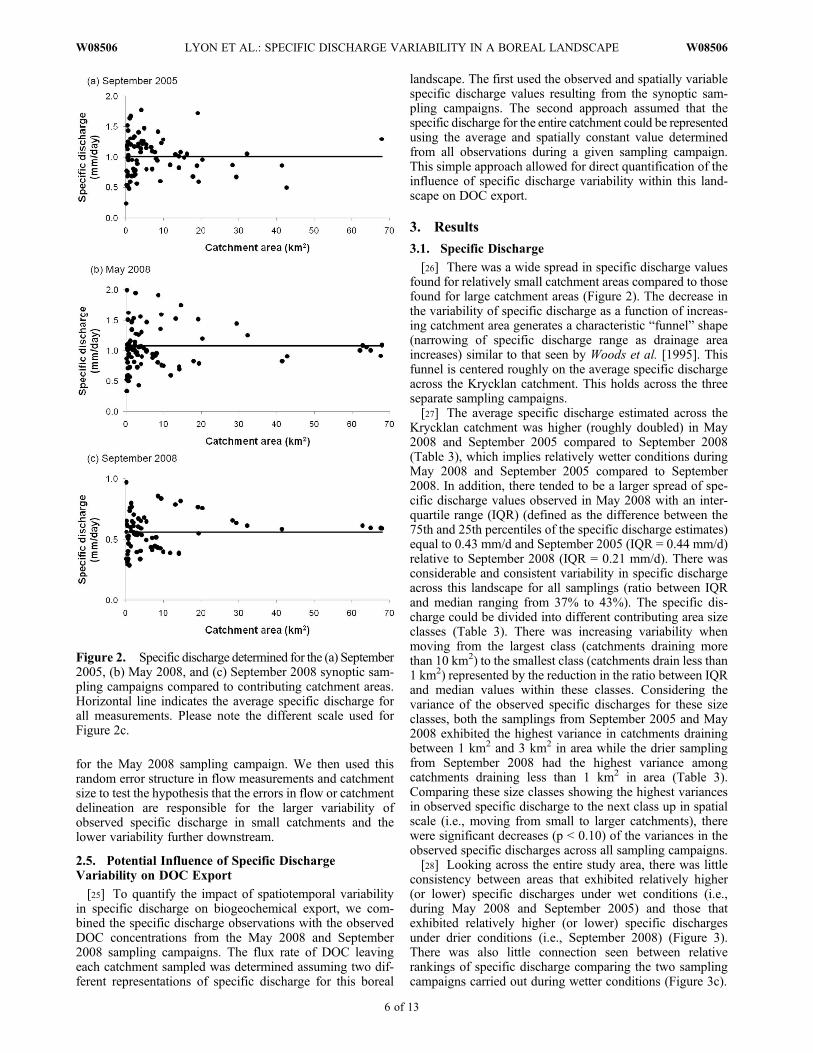
[26] There was a wide spread in specific discharge valuesfound for relatively small catchment areas compared to thosefound for large catchment areas (Figure 2). The decrease inthe variability of specific discharge as a function of increas-ing catchment area generates a characteristic “funnel” shape(narrowing of specific discharge range as drainage areaincreases) similar to that seen by Woods et al. [1995]. Thisfunnel is centered roughly on the average specific dischargeacross the Krycklan catchment. This holds across the threeseparate sampling campaigns.[27] The average specific discharge estimated across the

Krycklan catchment was higher (roughly doubled) in May2008 and September 2005 compared to September 2008(Table 3), which implies relatively wetter conditions duringMay 2008 and September 2005 compared to September2008. In addition, there tended to be a larger spread of spe-cific discharge values observed in May 2008 with an inter-quartile range (IQR) (defined as the difference between the75th and 25th percentiles of the specific discharge estimates)equal to 0.43 mm/d and September 2005 (IQR = 0.44 mm/d)relative to September 2008 (IQR = 0.21 mm/d). There wasconsiderable and consistent variability in specific dischargeacross this landscape for all samplings (ratio between IQRand median ranging from 37% to 43%). The specific dis-charge could be divided into different contributing area sizeclasses (Table 3). There was increasing variability whenmoving from the largest class (catchments draining morethan 10 km2) to the smallest class (catchments drain less than1 km2) represented by the reduction in the ratio between IQRand median values within these classes. Considering thevariance of the observed specific discharges for these sizeclasses, both the samplings from September 2005 and May2008 exhibited the highest variance in catchments drainingbetween 1 km2 and 3 km2 in area while the drier samplingfrom September 2008 had the highest variance amongcatchments draining less than 1 km2 in area (Table 3).Comparing these size classes showing the highest variancesin observed specific discharge to the next class up in spatialscale (i.e., moving from small to larger catchments), therewere significant decreases (p < 0.10) of the variances in theobserved specific discharges across all sampling campaigns.[28] Looking across the entire study area, there was little

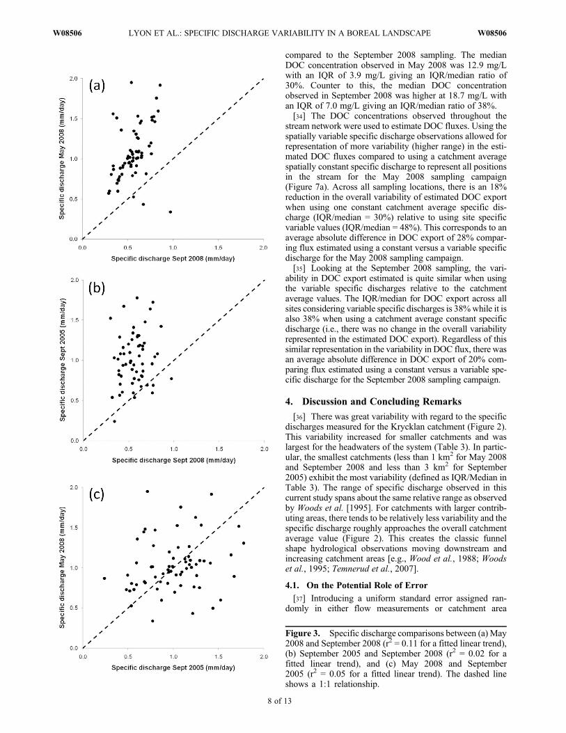
consistency between areas that exhibited relatively higher(or lower) specific discharges under wet conditions (i.e.,during May 2008 and September 2005) and those thatexhibited relatively higher (or lower) specific dischargesunder drier conditions (i.e., September 2008) (Figure 3).There was also little connection seen between relativerankings of specific discharge comparing the two samplingcampaigns carried out during wetter conditions (Figure 3c).

Figure 2. Specific discharge determined for the (a) September2005, (b) May 2008, and (c) September 2008 synoptic sam-pling campaigns compared to contributing catchment areas.Horizontal line indicates the average specific discharge forall measurements. Please note the different scale used forFigure 2c.


6 of 13

3.2. Landscape Interactions and Factor Analysis

[29] FA (Figure 4a) demonstrated that during the rela-tively drier September 2008 sampling the specific dischargeof streams in the Krycklan study catchment were positivelyrelated to both the area of wetlands and the average elevationwhile it was inversely related to potential annual evapora-tion. This is seen by the common orientation and distancefrom the origin of these characteristics along one of the mainfactor axes. The May 2008 and September 2005 specificdischarges, however, were less related to these (or other)landscape characteristics.[30] To test if relationships between landscape and spe-

cific discharge changed moving from large to small catch-ments (and explore statistical independence among theheadwaters), FA was repeated for progressively smallersubsets of catchments defined by contributing areas less than10 km2 (Figure 4b) and less than 3 km2 (Figure 4c). Therewas a consistent direct relationship between percentage ofwet areas and average elevation and inverse relationship withpotential annual evaporation for the September 2008 cam-paign when looking at smaller catchments. The relationshipof specific discharge to these characteristics in smallercatchments were weaker in both May 2008 and September2005, when soils were wetter and specific discharges werehigher. It should be noted that under the criterion consideredin this study, the percentage till characteristic was neverincluded in any of the final FA variable sets.[31] The results of the FA can be further illustrated

through simple regression (Figure 5). Clearly, there is apositive relationship between percentage wet areas andspecific discharge and a negative relationship betweenpotential annual evaporation and specific discharge duringthe relatively drier September 2008 sampling. While thegeneral trends for such relationships remained, their strength

decreases for either the May 2008 or September 2005 spe-cific discharges (similar to what was seen in the FA).

3.3. Potential Influence of Flow Measurementand Catchment Area Calculation Errors

[32] To test whether measurement errors were responsiblefor larger between-catchment variation in specific dischargefor smaller catchments than larger catchments, the mean andstandard deviation of errors in flow measurement or catch-ment area delineation were determined (Table 4). The singlesize of error (either absolute or relative) in flow optimized toreproduce the variability for the entire catchment was 3 L s�1

or 2%. The error in catchment delineation was 10 ha or 1%.The single optimized error value, however, did not success-fully represent the pattern of variation in specific discharge asa function of catchment size (r2 of 0.01 to 0.02 in Table 4 andFigure 6). When considering four separate catchment sizeclasses, the size of the random errors needed to reproduce thespecific discharge variability within each size class variedacross the four catchment size classes (Table 4). The abso-lute/relative error in flow varied from 2 L s�1/41% in thesmallest catchments to 80 L s�1/18% in the largest size class.The absolute/relative error in delineating catchment sizevaried from 10 ha/19% in the smallest catchments to 230 ha/7% in the largest size class. Combining these different opti-mized random errors across the different size classes it waspossible to better reproduce the variability in observed spe-cific discharge for the May 2008 campaign than when using aconstant error for all size classes (Figure 6).

3.4. Potential Influence of Specific DischargeVariability on DOC Export

[33] Observed DOC concentrations in the stream watersampling demonstrated less variability across the Krycklancatchment study area during the May 2008 sampling

Table 3. Summary Statistics of Specific Discharges From the Three Synoptic Sampling Campaigns in the Krycklan Catchment StudyAreaa

CampaignNumber ofCatchments

Average(mm/d)

Median(mm/d)

Standard Deviation(mm/d)

Optimized Variance(mm/d)2 IQR (mm/d) IQR/Median

All CatchmentsSeptember 2005 78 1.01 1.01 0.32 0.10 0.44 43%May 2008 84 1.08 1.01 0.41 0.17 0.43 43%September 2008 72 0.56 0.56 0.15 0.02 0.21 37%

Catchments > 10 km2

September 2005 18 0.94 0.91 0.28 0.08 0.22 24%May 2008 20 1.06 1.01 0.32 0.10 0.40 40%September 2008 17 0.61 0.61 0.14 0.02 0.10 17%

10 km2 > Catchments > 3 km2


3 km2 > Catchments > 1 km2


1 km2 > CatchmentsSeptember 2005 19 0.89 0.95 0.35 0.12 0.54 57%May 2008 24 0.95 0.95 0.39 0.15 0.45 47%September 2008 17 0.49 0.49 0.18 0.03 0.23 48%

aFurther, the specific discharges are divided into groupings by catchment contributing area. IQR is the interquartile range taken as the difference betweenthe 75th and 25th percentiles of the specific discharge estimates.


7 of 13

compared to the September 2008 sampling. The medianDOC concentration observed in May 2008 was 12.9 mg/Lwith an IQR of 3.9 mg/L giving an IQR/median ratio of30%. Counter to this, the median DOC concentrationobserved in September 2008 was higher at 18.7 mg/L withan IQR of 7.0 mg/L giving an IQR/median ratio of 38%.[34] The DOC concentrations observed throughout the

stream network were used to estimate DOC fluxes. Using thespatially variable specific discharge observations allowed forrepresentation of more variability (higher range) in the esti-mated DOC fluxes compared to using a catchment averagespatially constant specific discharge to represent all positionsin the stream for the May 2008 sampling campaign(Figure 7a). Across all sampling locations, there is an 18%reduction in the overall variability of estimated DOC exportwhen using one constant catchment average specific dis-charge (IQR/median = 30%) relative to using site specificvariable values (IQR/median = 48%). This corresponds to anaverage absolute difference in DOC export of 28% compar-ing flux estimated using a constant versus a variable specificdischarge for the May 2008 sampling campaign.[35] Looking at the September 2008 sampling, the vari-

ability in DOC export estimated is quite similar when usingthe variable specific discharges relative to the catchmentaverage values. The IQR/median for DOC export across allsites considering variable specific discharges is 38%while it isalso 38% when using a catchment average constant specificdischarge (i.e., there was no change in the overall variabilityrepresented in the estimated DOC export). Regardless of thissimilar representation in the variability in DOC flux, there wasan average absolute difference in DOC export of 20% com-paring flux estimated using a constant versus a variable spe-cific discharge for the September 2008 sampling campaign.

4. Discussion and Concluding Remarks

[36] There was great variability with regard to the specificdischarges measured for the Krycklan catchment (Figure 2).This variability increased for smaller catchments and waslargest for the headwaters of the system (Table 3). In partic-ular, the smallest catchments (less than 1 km2 for May 2008and September 2008 and less than 3 km2 for September2005) exhibit the most variability (defined as IQR/Median inTable 3). The range of specific discharge observed in thiscurrent study spans about the same relative range as observedby Woods et al. [1995]. For catchments with larger contrib-uting areas, there tends to be relatively less variability and thespecific discharge roughly approaches the overall catchmentaverage value (Figure 2). This creates the classic funnelshape hydrological observations moving downstream andincreasing catchment areas [e.g., Wood et al., 1988; Woodset al., 1995; Temnerud et al., 2007].

4.1. On the Potential Role of Error

[37] Introducing a uniform standard error assigned ran-domly in either flow measurements or catchment area

Figure 3. Specific discharge comparisons between (a) May2008 and September 2008 (r2 = 0.11 for a fitted linear trend),(b) September 2005 and September 2008 (r2 = 0.02 for afitted linear trend), and (c) May 2008 and September2005 (r2 = 0.05 for a fitted linear trend). The dashed lineshows a 1:1 relationship.


8 of 13

calculations across the entire range of catchment sizes couldnot produce results similar to those seen in this study, i.e., adecrease in specific discharge variability with increase inarea. To achieve the observed results, different error dis-tributions and thus standard errors were needed for differentsize classes of contributing areas (Figure 6). Dividing the

catchments into four size classes and optimizing a standarderror in flow or area delineation made it possible to reproducethe characteristic “funnel” shape in specific discharge vari-ability versus area. But the errors needed in flow were not inagreement with the potential size of these errors. A 40% errorin flow measurement on the small catchments, or even aroughly 30% error on the 1 km2 to 10 km2 catchments(Table 4) is not realistic. The errors in flow needed to give thepatterns of variability in specific discharge are greater thanestimated from repeated flow measurements (about 5%).[38] The relative error representing these optimized stan-

dard errors can be put into perspective by comparison withthe confidence intervals provided in the study by Woodset al. [1995]. From their Figure 4, for flows approximatelyof the same order of magnitude seen at Krycklan (about5–500 L s�1) one would roughly expect about 5% to 10%of error associated with measuring of flow. Such “real”relative error values in flow measurements are much lowerthan those optimized values (Table 4) needed to create thespecific discharge funnel shape (Figure 6). As such, it isunlikely that the pattern seen between specific dischargeand area is due to error.[39] The plausibility of the errors in catchment delineation

required to reproduce the variation in the 4 size classes (7% to19% from Table 4) are less well documented. A 20% errorin catchment area might be possible for those catchments<1 km2 or those from 1 km2 to 3 km2 (Table 4). But ifthere were an error in catchment area, then one wouldexpect the catchments with higher estimated specific dis-charges due to this error would remain consistently highacross all sampling campaigns. This was not the case of theobservations, since the small catchments with relativelyhigh and low specific discharge relative to the mean variedbetween the three campaigns. This suggests that catchmentsize errors are not the source of the variability in specificdischarge between the smaller catchments (e.g., Figure 3).

4.2. Temporal Variability in Specific Discharge Acrossthe Landscape

[40] In late spring (May 2008) this boreal landscape isextremely wet due to previously near-saturated conditionsduring spring freshet. As the landscape transitions fromspring through summer into autumn (September 2008), adrier landscape emerges (Figure 3a). This has been observedas a reduction in variability of shallow groundwater tablebetween May 2008 and September 2008 in the Krycklancatchment study area [Grabs, 2010; Lyon et al., 2011]. Thedistribution of wet areas and potential evaporation withelevation are the main landscape characteristics determiningthe emergence of specific discharge patterns as this boreallandscape moves from wet to dry conditions over the sum-mer (Figures 4 and 5). This is consistent with transpirationfrom the forest stands in this boreal system promoting the“drying out” of the landscape through the summer period.This is counteracted by the wet areas, which tend to increasewith elevation, and appear to keep parts of the landscaperelatively wetter through the summer.[41] Under rewetting conditions (e.g., September 2005),

however, this is negated and the relationship between drycondition specific discharges and landscape that developedover the summer months diminishes (Figure 4). Thisrewetting, however, may not result in exactly the samespatial distribution of specific discharge as that observed

Figure 4. Factor analysis showing the multivariate rela-tions between the landscape characteristics in Table 1 andthe synoptically observed specific discharges from the threecampaigns for the specific discharges across (a) all catch-ments, (b) those less than 10 km2, and (c) those less than3 km2. The number in parentheses on each axis indicatestotal variance explained by each factor.


9 of 13

Figure 5. Relationship between specific discharge and percentage wet areas in catchments for(a) September 2005, (b) May 2008, and (c) September 2008 and between specific discharge and potentialannual evaporation for (d) September 2005, (e) May 2008, and (f) September 2008.

Table 4. Standard Errors Needed to Reproduce the Specific Discharge Variability From FlowMeasurements or Catchment Area CalculationsAcross the Entire Krycklan Catchment Study Area and the Size Classes Considered in the May 2008 Sampling Campaigna

Size ClassNumber ofCatchments

AverageFlow(L/s)

AverageArea(km2)

StandardDeviationof Flow(L/s)

StandardDeviationof Area(km2)

StandardError Needed

in Flow(L/s)

Standard ErrorNeeded inArea (km2)

Error ofAverageFlow

Error ofAverageArea

Flow ErrorModel r2

Area ErrorModel r2

All 84 126.2 9.9 210.3 17.7 3 0.1 2% 1% 0.02 0.01>10 km2 19 433.0 35.4 263.4 22.5 80 2.3 18% 7% 0.02 0.263 km2 to 10 km2 26 71.2 6.0 41.9 2.4 20 0.6 28% 10% 0.19 0.051 km2 to 3 km2 15 26.1 1.9 10.8 0.6 9 0.4 34% 21% 0.02 0.01<1 km2 24 5.6 0.5 3.0 0.2 2 0.1 41% 19% 0.02 0.03

aThe Flow and Area error model r2 are for the observations against the respective standard error models.


10 of 13

during wet conditions at the end of the spring freshet(May 2008) (Figure 3c). This is also seen by the relationshipbetween the September 2005 synoptic campaign and the May2008 synoptic campaign in the FA (Figure 4a).[42] As such, the results of this study clearly indicate the

ability of forests to dry out parts of the catchment over thesummer months while wetlands keep wet other parts in thisboreal landscape (Figure 5). Such control of the landscapeforms a potential organizing principle [i.e.,McDonnell et al.,2007] governing (to some extent) process complexity duringpart of the year [e.g., Harpold et al., 2010; Jencso et al.,2010; McDaniel et al., 2008; Spence et al., 2010;McNamara et al., 2005]. This raises hope for characterizingsimilarity and modeling hydrologic response across scales in

these headwater boreal systems. But it also underlines theimportance of considering the variability of specific dis-charge in studies of landscape export as patterns in flow maybe associated with patterns in concentration that could leadto errors when estimating landscape exports with differentconcentrations across the landscape, but uniform specificdischarge.

4.3. Implications for Transport and BiogeochemicalFlux Modeling

[43] The specific discharge spatial variability found inthis current study has important implications for biogeo-chemical transport monitoring and modeling. Consider thecase of DOC export from these boreal systems. Large

Figure 6. Error analysis model simulations (white symbols) assuming random error in (a) flow measure-ments or (b) catchment area calculations needed to reproduce the observed specific discharge for May2008 (black symbols) determined in this study. The simulations here are the final averaged “realizations”that give the same pattern of specific discharge across scales observed in May 2008. Table 4 has the finaloptimized standard error values. The gray symbols show the pattern of specific discharge assuming a uni-form random error across all scales. Horizontal dashed lines correspond to the size classes considered.


11 of 13

spatial variability in DOC soil water concentrations [Grabs,2010; Lyon et al., 2011] and stream water concentrations[Buffam et al., 2007; Temnerud and Bishop, 2005] have beenobserved across this and many other boreal systems. As such,estimating organic carbon (or other biogeochemical) exportsusing a uniform specific discharge will potentially lead toinaccurate export values if there is a nonrandom relationbetween specific discharge and concentrations at any givenpoint in time in the catchment [Temnerud et al., 2007]. Thisis explicitly demonstrated in this study (Figure 7) whereusing the uniform specific discharge lead to 20–28% averageabsolute error in DOC export. Further, for the samplingsconsidered in this study, the spatial variability in specificdischarge appears to have a larger influence on the variabilityof estimated DOC flux under wet conditions (May 2008 andFigure 7a) than relatively drier conditions (September 2008and Figure 7b).[44] Clearly, as demonstrated by the current study,

adopting one uniform specific discharge value at the catch-ment scale is troublesome and would not allow for capturingthe full extent of the spatial variability present in the system.This is consistent with the general interactions seen between

temporally varying flow-generating zones that mobilizespatially distributed source zones [Basu et al., 2010] or thespecific interactions seen in Krycklan between ripariansource zones and temporal water table fluctuations [Seibertet al., 2009]. Still, there appears to be some connectionbetween specific discharge and the landscape for part of theyear (Figure 4). This provides some basic organizing prin-ciples around which to quantify the current state of hydro-logical processes in this boreal landscape. The combinedroles of forests and wet areas, for example, create landscapefactors that are “latent” under wet conditions (e.g., May2008 and/or September 2005) and more “patent” in drierconditions (e.g., September 2008).[45] The understanding of current interactions between

landscape and hydrologic response in boreal systems iscrucial to the development of effective and efficient futuremanagement scenarios that must both consider streamflowconditions at ungauged locations and allow for interpretationof hydrochemical behavior [Buttle and Eimers, 2009]. Thisis particularly true with regards to estimating chemicalfluxes (e.g., DOC) from current and potential future borealforested landscapes.

[46] Acknowledgments. The lead author (S.L.) acknowledges supportin the form of funding from the Swedish Research Council (VR) and the BertBolin Centre for Climate Research (BBCC), which is supported by a Linnaeusgrant from VR and the Swedish Research Council Formas, and funding fromVR (grant 2011-4390). We also acknowledge the support to the Krycklancatchment study from VR (grant 2005-4289), Formas (ForWater), FutureForests, SKB and Elforsk-HUVA. M.N. thanks the Ministry of Educationand Research of the Swedish Government and the Education Administrationat the City of Stockholm for support in the form of funding. Some data usedhere are from the Swedish Meteorological and Hydrological Institute (SMHI)and were produced with support from the Swedish Radiation ProtectionAuthority and the Swedish Environmental Agency. Forest vegetation dataused in this study were kindly provided by the Department of Forest ResourceManagement, Swedish University of Agricultural Sciences. Anton Lindahl,Anneli Ågren, and the entire Krycklan catchment study crew for help withsampling and GIS analysis.

ReferencesÅgren, A., I. Buffam, M. Jansson, and H. Laudon (2007), Importance of sea-sonality and small streams for the landscape regulation of dissolved organiccarbon export, J. Geophys. Res., 112, G03003, doi:10.1029/2006JG000381.

Asano, Y., and T. Uchida (2010), Is representative elementary area definedby a simple mixing of variable small streams in headwater catchments?,Hydrol. Processes, 24, 666–671, doi:10.1002/hyp.7589.

Basu, N. B., et al. (2010), Nutrient loads exported from managed catch-ments reveal emergent biogeochemical stationarity, Geophys. Res. Lett.,37, L23404, doi:10.1029/2010GL045168.

Bergknut, M., S. Meijer, C. Halsall, A. Agren, H. Laudon, S. Kohler, K. C.Jones, M. Tysklind, and K.Wiberg (2010),Modelling the fate of hydropho-bic organic contaminants in a boreal forest catchment: A cross disciplinaryapproach to assessing diffuse pollution to surface waters, Environ. Pollut.,158, 2964–2969, doi:10.1016/j.envpol.2010.05.027.

Beven, K. J., and M. J. Kirkby (1979), Towards a simple, physically based,variable contributing area model of catchment hydrology, IAHS Bull., 24,43–69, doi:10.1080/02626667909491834.

Bishop, K. H., H. Grip, and A. O’Neill (1990), The origins of acid runoff ina hillslope during storm events, J. Hydrol., 116, 35–61, doi:10.1016/0022-1694(90)90114-D.

Bishop, K., I. Buffam, M. Erlandsson, J. Fölster, H. Laudon, J. Seibert, andJ. Temnerud (2008), Aqua incognita: The unknown headwaters, Hydrol.Processes, 22, 1239–1242, doi:10.1002/hyp.7049.

Björkvald, L., I. Buffam, H. Laudon, and C. M. Mörth (2008), Hydrogeo-chemistry of Fe and Mn in small boreal catchments: The role of sea-sonality, landscape type and scale, Geochim. Cosmochim. Acta, 72,2789–2804, doi:10.1016/j.gca.2008.03.024.

Böhner, J., T. Blaschke, and L. Montanarella (Eds.) (2008), SAGA: Systemfor an Automated Geographical Analysis,Hamburger Beitr. Phys. Geogr.

Figure 7. Dissolved organic carbon (DOC) flux estimatedfor the (a) May 2008 and (b) September 2008 sampling cam-paigns assuming either variable specific discharge (blacksymbols) or constant specific discharge (white symbols)across the Krycklan catchment study area.


12 of 13

Landschaftsökol. 19, Inst. of Geogr., Univ. of Hamburg, Hamburg,Germany.

Buffam, I., H. Laudon, J. Temnerud, C. M. Mörth, and K. Bishop (2007),Landscape-scale variability of acidity and dissolved organic carbon dur-ing spring flood in a boreal stream network, J. Geophys. Res., 112,G01022, doi:10.1029/2006JG000218.

Buttle, J. M., and M. C. Eimers (2009), Scaling and physiographic controlson streamflow behavior on the Precambrian Shield, south-centralOntario, J. Hydrol., 374, 360–372, doi:10.1016/j.jhydrol.2009.06.036.

Conrad, O. (2007), SAGA—Entwurf, Funktionsumfang und Anwendungeines Systems für Automatisierte Geowissenschaftliche Analysen, elec-tronic doctoral dissertation thesis, 221 pp., Univ. of Göttingen, Göttingen,Germany.

Costello, A. B., and J. W. Osborne (2005), Best practices in exploratoryfactor analysis: Four recommendations for getting the most from youranalysis, Pract. Assess. Res. Eval., 10(7), 1–9.

Day, T. J. (1977), Observed mixing lengths in mountain streams, J. Hydrol.,35(1–2), 125–136, doi:10.1016/0022-1694(77)90081-6.

Didszun, J., and S. Uhlenbrook (2008), Scaling of dominant runoff genera-tion processes: Nested catchments approach using multiple tracers,WaterResour. Res., 44, W02410, doi:10.1029/2006WR005242.

Gauch, H. G. (1982), Multivariate Analysis in Community Ecology,289 pp., Cambridge Univ. Press, Cambridge, U. K.

Grabs, T. (2010), Water quality modeling based on landscape analysis:Importance of riparian hydrology, Ph.D. thesis, Stockholm Univ.,Stockholm.

Grabs, T., J. Seibert, K. Bishop, and H. Laudon (2009), Modeling spatialpatterns of saturated areas: A comparison of the topographic wetnessindex and a dynamic distributed model, J. Hydrol., 373, 15–23,doi:10.1016/j.jhydrol.2009.03.031.

Grabs, T., K. G. Jencso, B. L. McGlynn, and J. Seibert (2010), Calculatingterrain indices along streams: A new method for separating stream sides,Water Resour. Res., 46, W12536, doi:10.1029/2010WR009296.

Grayson, R. B., C. J. Gippel, B. L. Finlayson, and B. T. Hart (1997),Catchment-wide impacts on water quality: The use of ‘snapshot’ sam-pling during stable flow, J. Hydrol., 199(1–2), 121–134, doi:10.1016/S0022-1694(96)03275-1.

Haei, M., M. G. Öquist, I. Buffam, A. Ågren, P. Blomkvist, K. Bishop,M. Ottosson Löfvenius, and H. Laudon (2010), Cold winter soilsenhance dissolved organic carbon concentrations in soil and streamwater, Geophys. Res. Lett., 37, L08501, doi:10.1029/2010GL042821.

Harpold, A. A., S. W. Lyon, P. A. Troch, and T. S. Steenhuis (2010), Thehydrological effects of lateral preferential flow paths in a glaciated water-shed in the northeastern USA, Vadose Zone J., 9, 397–414, doi:10.2136/vzj2009.0107.

Hornberger, G. M., and E. W. Boyer (1995), Recent advances in watershedmodeling, U.S. Natl. Rep. Int. Union Geod. Geophys. 1991–1994, Rev.Geophys., 33, 949–957, doi:10.1029/95RG00288.

Hrachowitz, M., C. Soulsby, D. Tetzlaff, and M. Speed (2010), Catchmenttransit times and landscape controls—Does scale matter?,Hydrol. Processes,24, 117–125, doi:10.1002/hyp.7510.

Hudson, R., and J. Fraser (2005), Introduction to salt dilution gauging forstreamflow measurement, part IV: The mass balance (or dry injection)method, Streamline Watershed Manage. Bull., 9(1), 6–12.

Hyvönen, R., et al. (2007), The likely impact of elevated CO2, nitrogendeposition, increased temperature and management on carbon sequestra-tion in temperate and boreal forest ecosystems: A literature review, NewPhytol., 173, 463–480, doi:10.1111/j.1469-8137.2007.01967.x.

Jencso, K. G., B. L. McGlynn, M. N. Gooseff, K. E. Bencala, and S. M.Wondzell (2010), Hillslope hydrologic connectivity controls ripariangroundwater turnover: Implications of catchment structure for riparianbuffering and stream water sources, Water Resour. Res., 46, W10524,doi:10.1029/2009WR008818.

Klemeš, V. (1986), Dilettantism in hydrology: Transition or destiny, WaterResour. Res., 22, 177S–188S, doi:10.1029/WR022i09Sp0177S.

Köhler, S. J., I. Buffam, H. Laudon, and K. H. Bishop (2008), Climate’scontrol of intra-annual and interannual variability of total organic carbonconcentration and flux in two contrasting boreal landscape elements,J. Geophys. Res., 113, G03012, doi:10.1029/2007JG000629.

Laudon, H., V. Sjöblom, I. Buffam, J. Seibert, and M. Mörth (2007), Therole of catchment scale and landscape characteristics for runoff generation ofboreal streams, J. Hydrol., 344, 198–209, doi:10.1016/j.jhydrol.2007.07.010.

Laudon, H., M. Berggren, A. Ågren, I. Buffam, K. Bishop, T. Grabs,M. Jansson, and S. Köhler (2011), Patterns and dynamics of dissolvedorganic carbon (DOC) in boreal streams: The role of processes,

connectivity and scaling, Ecosystems, 14(6), 880–893, doi:10.1007/s10021-011-9452-8.

Lindgren, G. A., S. Wrede, J. Seibert, and M. Wallin (2007), Nitrogensource apportionment modeling and the effect of land-use class relatedrunoff contributions, Nord. Hydrol., 38(4–5), 317–331, doi:10.2166/nh.2007.015.

Lohse, K. A., P. D. Brooks, J. C. McIntosh, T. Meixner, and T. E. Huxman(2009), Interactions between biogeochemistry and hydrologic systems,Annu. Rev. Environ. Resour., 34, 65–96, doi:10.1146/annurev.environ.33.031207.111141.

Lyon, S. W., H. Laudon, J. Seibert, M. Mörth, D. Tetzlaff, and K. H. Bishop(2010), Controls on snowmelt water mean transit times in northern borealcatchments, Hydrol. Processes, 24, 1672–1684, doi:10.1002/hyp.7577.

Lyon, S. W., T. Grabs, H. Laudon, K. H. Bishop, and J. Seibert (2011),Variability of groundwater levels and total organic carbon in the riparianzone of a boreal catchment, J. Geophys. Res., 116, G01020, doi:10.1029/2010JG001452.

Maidment, D. R. (Ed.) (1992), Handbook of Hydrology, McGraw-Hill,New York.

McDaniel, P. A., M. P. Regan, E. Brooks, J. Boll, S. Barndt, A. Falen, S. K.Young, and J. E. Hammel (2008), Linking fragipans, perched water tables,and catchment scale hydrological processes, Catena, 73, 166–173,doi:10.1016/j.catena.2007.05.011.

McDonnell, J. J., et al. (2007), Moving beyond heterogeneity and processcomplexity: A new vision for watershed hydrology, Water Resour.Res., 43, W07301, doi:10.1029/2006WR005467.

McNamara, J. P., D. Chandler,M. Seyfried, and S. Achet (2005), Soil moisturestates, lateral flow, and streamflow generation in a semi-arid, snowmelt-drivencatchment, Hydrol. Processes, 19, 4023–4038, doi:10.1002/hyp.5869.

Salvia, M., J. F. Iffly, P. Vander Borght, M. Sary, and L. Hoffmann (1999),Application of the ‘snapshot’ methodology to a basin-wide analysis ofphosphorus and nitrogen at stable low flow, Hydrobiologia, 410, 97–102,doi:10.1023/A:1003892830838.

Seibert, J., and B. McGlynn (2007), A new triangular multiple flow direc-tion algorithm for computing upslope areas from gridded digital elevationmodels, Water Resour. Res., 43, W04501, doi:10.1029/2006WR005128.

Seibert, J., T. Grabs, S. Kohler, H. Laudon, M. Winterdahl, and K. Bishop(2009), Linking soil- and stream-water chemistry based on a riparianflow-concentration integration model, Hydrol. Earth Syst. Sci., 13,2287–2297, doi:10.5194/hess-13-2287-2009.

Shaman, J., M. Stieglitz, and D. Burns (2004), Are big basins just the sumof small catchments?, Hydrol. Processes, 18, 3195–3206, doi:10.1002/hyp.5739.

Spence, C., X. J. Guan, R. Phillips, N. Hedstrom, R. Granger, and B. Reid(2010), Storage dynamics and streamflow in a catchment with a variablecontributing area, Hydrol. Processes, 24, 2209–2221, doi:10.1002/hyp.7492.

Temnerud, J., and K. Bishop (2005), Spatial variation of stream water chem-istry in two Swedish boreal catchments: Implications for environmentalassessment, Environ. Sci. Technol., 39(6), 1463–1469, doi:10.1021/es040045q.

Temnerud, J., J. Seibert, M. Jansson, and K. Bishop (2007), Spatial varia-tion in discharge and concentrations of organic carbon in a catchmentnetwork of boreal streams in northern Sweden, J. Hydrol., 342(1–2),72–87, doi:10.1016/j.jhydrol.2007.05.015.

Uchida, T., Y. Asano, Y. Onda, and S. Miyata (2005), Are headwaters justthe sum of hillslopes?, Hydrol. Processes, 19, 3251–3261, doi:10.1002/hyp.6004.

Wagener, T., M. Sivapalan, P. A. Troch, B. L. McGlynn, C. J. Harman,H. V. Gupta, P. Kumar, P. S. C. Rao, N. B. Basu, and J. S. Wilson(2010), The future of hydrology: An evolving science for a changingworld, Water Resour. Res., 46, W05301, doi:10.1029/2009WR008906.

Wolock, D. M., J. Fan, and G. B. Lawrence (1997), Effects of basin size onlow-flow stream chemistry and subsurface contact time in the Neversink Riverwatershed, New York,Hydrol. Processes, 11, 1273–1286, doi:10.1002/(SICI)1099-1085(199707)11:9<1273::AID-HYP557>3.0.CO;2-S.

Wood, E. F., M. Sivapalan, K. Beven, and L. Band (1988), Effects of spatialvariability and scale with implications to hydrologic modeling,J. Hydrol., 102, 29–47, doi:10.1016/0022-1694(88)90090-X.

Woods, R., M. Sivapalan, and M. Duncan (1995), Investigating the repre-sentative elementary area concept: An approach based on field data,Hydrol. Processes, 9, 291–312, doi:10.1002/hyp.3360090306.

Xu, C. Y., and V. P. Singh (2000), Evaluation and generalization ofradiation-based methods for calculating evaporation, Hydrol. Processes,14(2), 339–349, doi:10.1002/(SICI)1099-1085(20000215)14:2<339::AID-HYP928>3.0.CO;2-O.


13 of 13

zurichopenrepositoryand universityofzurich year: 2012

Documents