In this chapter we’ll learn about ‘confidence intervals.’

A confidence interval is a range that captures the ‘true value’ of a statistic with a specified probability (i.e. ‘confidence’).

Let’s figure out what this means.

To do so we need to continue exploring the principles of statistical inference: using samples to make estimates about a population.

See, e.g., King et al., Designing Social Inquiry, on the topic of inference.

Remember that fundamental to statistical inference are probability principles that allow us to answer the question: what would happen if we repeated this random sample many times, independently and under the same conditions?

According to the laws of probability, each independent, random sample of size-n from the same population yields the following:

true value +/- random error

The procedure, to repeat, must be a random sample or a randomized experiment (or, at very least, independent observations from a population) in order for probability to operate.

If not, the use of statistical inference is invalid.

Remember also that sample means are unbiased estimates of the population mean; & that the standard deviation of sample means can be made narrower by (substantially) increasing the size of random samples-n.

Further: remember that means are less variable & more normally distributed than individual observations.

If the underlying population distribution is normal, then the sampling distribution of the mean will also be normal.

There’s also the Law of Large Numbers.

And last but perhaps most important, there’s the Central Limit Theorem: given a simple random sample from a population with any distribution of x, when n is large the sampling distribution of sample means is approximately normal.

That is, in large samples weighted averages are distributed as normal variables.

The Central Limit Theorem allows us to use normal probability calculations to answer questions about sample means from many observations even when the population distribution is not normal.

Of course, the sample size must be large enough to do so.

N=30 is a common benchmark threshold for the Central Limit Theorem, but N=100 or more may be required, depending on the variability of the distribution.

Greater N is required with greater variability in the variable of interest (as well as to have sufficient observations to conduct hypothesis tests).

The Point of Departure for Inferential Statistics

Here, now, is the most basic problem in inferential statistics: you’ve drawn a random sample & estimated a sample mean.

How reliable is this estimate? After all, repeated random samples of the same sample size-n in the same population would be unlikely to give the same sample mean.

How do you know, then, where the sample mean obtained would be located in the variable’s sampling distribution: i.e. on its histogram displaying the sample means for all possible random samples of the same size-n in the same population?

Can’t we simply rely on the fact that the sample mean is an unbiased estimator of the population mean?

No, we can’t: that only says that the sample mean of a random sample has no systematic tendency to undershoot or overshoot the population mean.

We still don’t know if, e.g., the sample mean we obtained is at the very low end or the very high end of the histogram of the sampling distribution, or is located somewhere around the center.

In other words, a sample estimate without an indication of variability is of little value.

In fact, what’s the worst thing about a sample of just one observation?

Answer

A sample of one observation doesn’t allow us to estimate the variability of the sample mean over repeated random samples of the same size in the same population.

See Freedman et al., Statistics.

To repeat, a sample estimate without an indication of variability is of little value.

What must we do?

The solution has to do with a sample mean’s standard deviation, divided by the square root of the sample size-n.

Thus we compute the sample mean’s standard deviation & divide it by the square root of the sample size-n: this is called the standard error (see Moore/McCabe/Craig Chapter 7).

Introduction to Confidence Intervals

What does the result allow us to do?

It allows us to situate the sample mean’s variability within the sampling distribution of the sample mean: the distribution of sample means for all possible random samples of the same size from the same population.

It is the standard deviation of the sampling distribution of the sample mean (i.e. of the sample mean over repeated independent random samples of the same size & in the same population).

And it allows us to situate the sample mean’s variability in terms of the 68 – 95 – 99.7 Rule.

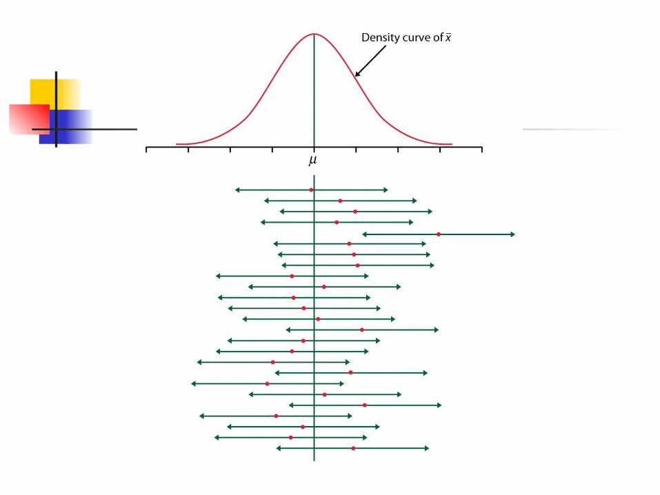
The probability is 68% that x-mean lies within +/- one standard deviation of the population mean (i.e. the true value); 95% that x-mean lies within +/- two standard deviations of the population mean; & 99.7% that x-mean lies within +/- three standard deviations of the population mean.

A common practice in statistics is to use the benchmark of +/- two standard deviations: i.e. a range likely to capture 95% of sample means obtained by repeated random samples of the same size-n in the same population.

We can therefore conclude: we’re 95% certain that this sample mean falls within +/- two standard deviations of the population mean—i.e. of the true population value.

Unfortunately, it also means that we still have room for worry: 5% of such samples will not obtain a sample mean within this range—i.e. will not capture the true population value.

The interval either captures the parameter (i.e. population mean) or it doesn’t.

What’s worse: we never know when the confidence interval captures the interval or not.

As Freedman et al. put it, a 95% confidence interval is “like buying a used car. About 5% turn out to be lemons.”

Recall that conclusions are always uncertain.

In any event, we’ve used our understanding of how the laws of probability work in the long run—with repeated random samples of size-n from the same population—to express a specified degree of confidence in the results of this one sample.

That is, the language of statistical inference uses the fact about what would happen in the long run to express our confidence in the results of any one random sample of independent observations.

If things are done right, this is how we interpret a 95% confidence interval: “This number was calculated by a method that captures the true population value in 95% of all possible samples.”

Again, it’s a range that captures the ‘true value’ of a statistic with a specified probability (i.e. confidence).

To repeat: the confidence interval either captures the parameter (i.e. the true population value) or it doesn’t—there’s no in between.

Warning!

A confidence interval addresses sampling error, but not non-sampling error.

What are the sources of non-sampling error?

Standard deviation vs. Standard error

Standard deviation: average deviation from the mean for a set of numbers.

Standard error: estimated average variation from the expected value of the sample mean for repeated, independent random samples of the same size & from the same population.

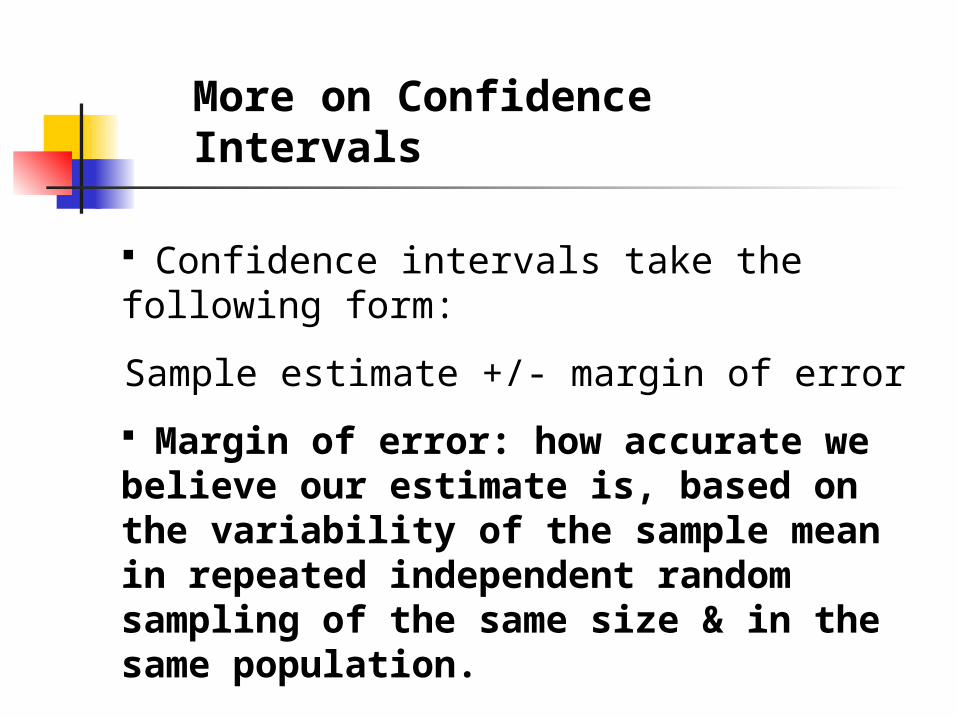
More on Confidence Intervals

Confidence intervals take the following form:

Sample estimate +/- margin of error

Margin of error: how accurate we believe our estimate is, based on the variability of the sample mean in repeated independent random sampling of the same size & in the same population.

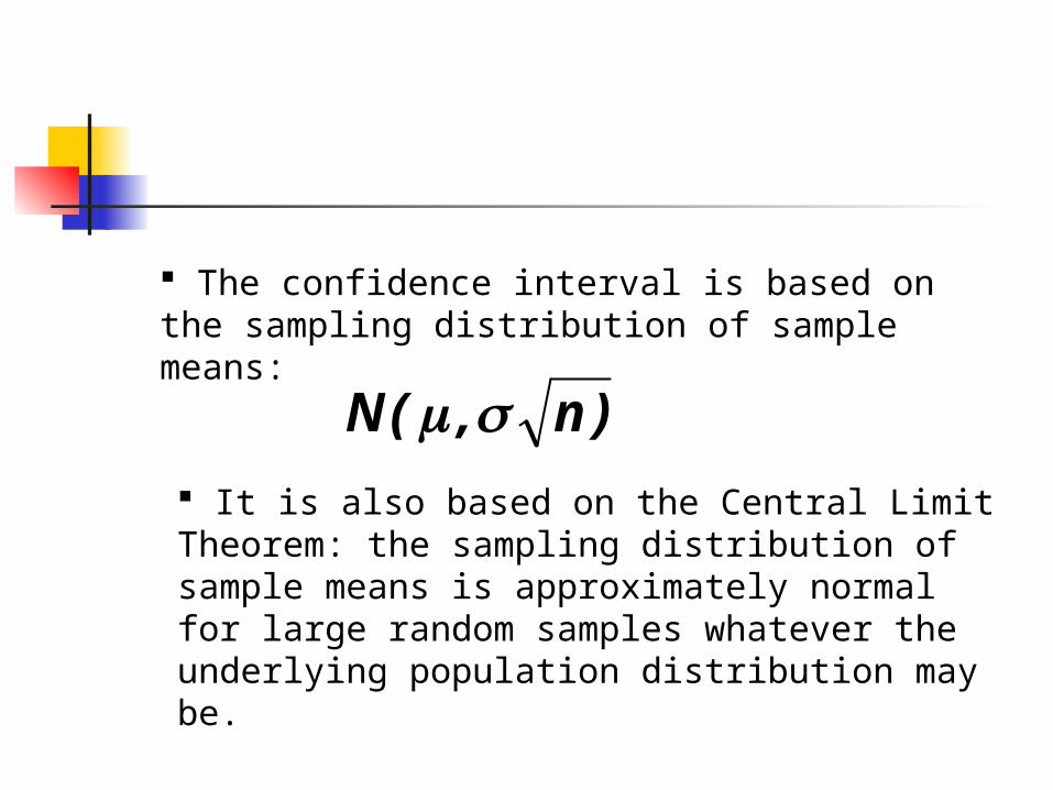
)n ,(N

The confidence interval is based on the sampling distribution of sample means:

It is also based on the Central Limit Theorem: the sampling distribution of sample means is approximately normal for large random samples whatever the underlying population distribution may be.

That is, what really matters is that the sampling distribution of sample means is normally distributed—not how the particular sample of observations is distributed (or whether the population distribution is normally distributed).

If the sample size is less than 30 or the assumption of population normality doesn’t hold, see Moore/McCabe/Craig on bootstrapping and Stata ‘help bootstrap’.

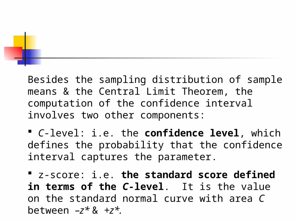
Besides the sampling distribution of sample means & the Central Limit Theorem, the computation of the confidence interval involves two other components:

C-level: i.e. the confidence level, which defines the probability that the confidence interval captures the parameter.

z-score: i.e. the standard score defined in terms of the C-level. It is the value on the standard normal curve with area C between –z* & +z*.

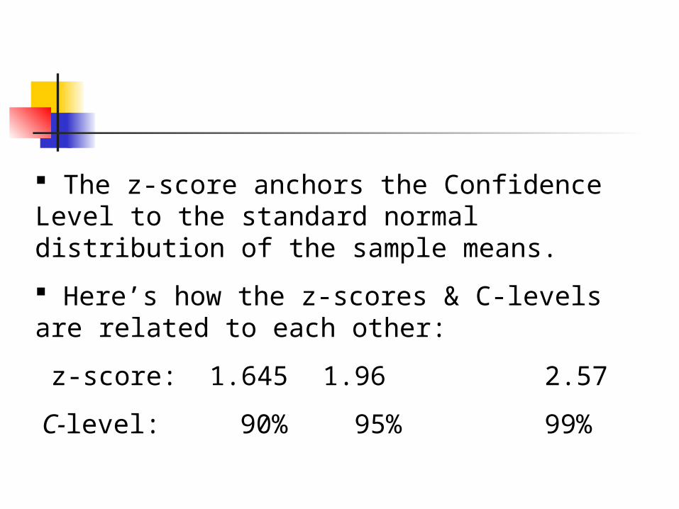
The z-score anchors the Confidence Level to the standard normal distribution of the sample means.

Here’s how the z-scores & C-levels are related to each other:

z-score: 1.645 1.96 2.57

C-level: 90% 95% 99%

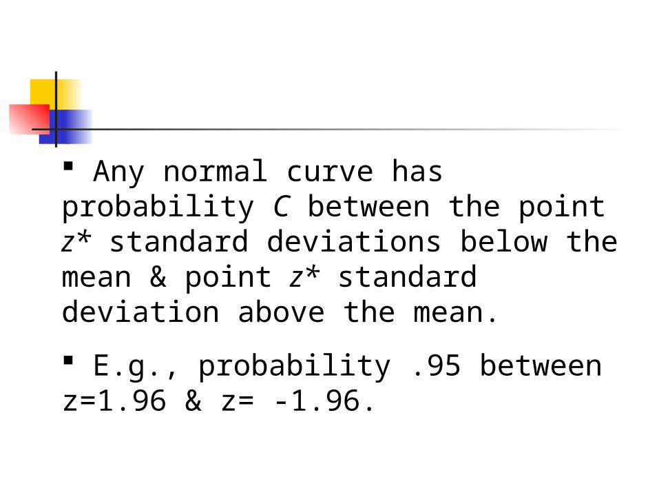
Any normal curve has probability C between the point z* standard deviations below the mean & point z* standard deviation above the mean.

E.g., probability .95 between z=1.96 & z= -1.96.

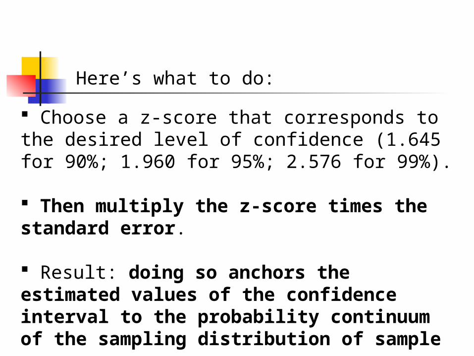
Here’s what to do:

Choose a z-score that corresponds to the desired level of confidence (1.645 for 90%; 1.960 for 95%; 2.576 for 99%).

Then multiply the z-score times the standard error. Result: doing so anchors the estimated values of the confidence interval to the probability continuum of the sampling distribution of sample means.

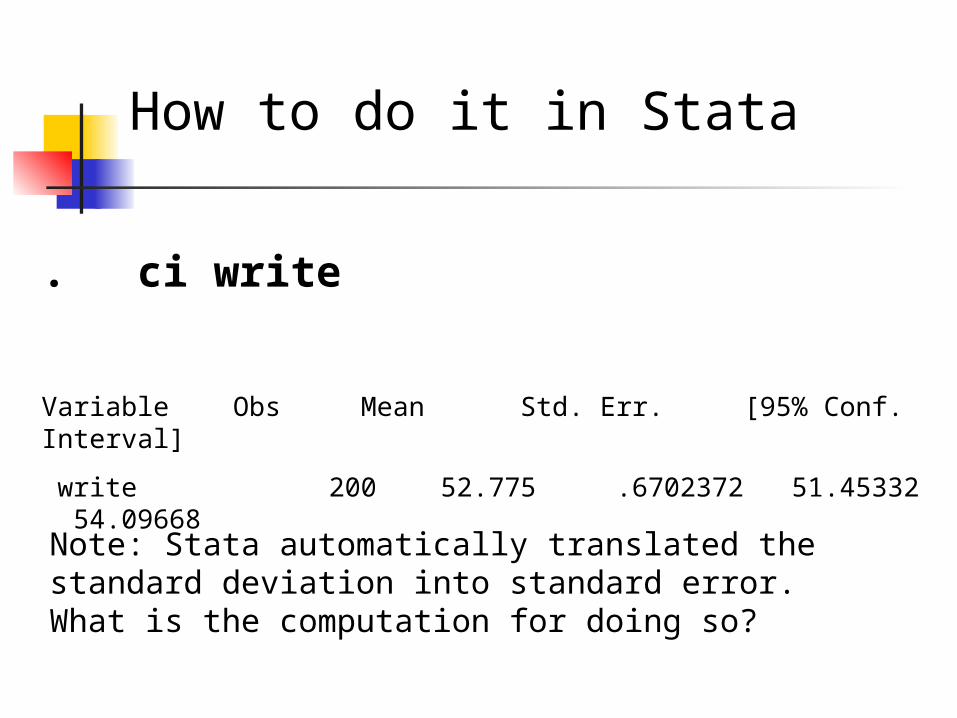
How to do it in Stata

. ci write

Variable Obs Mean Std. Err. [95% Conf. Interval]

write 200 52.775 .6702372 51.45332 54.09668

Note: Stata automatically translated the standard deviation into standard error. What is the computation for doing so?

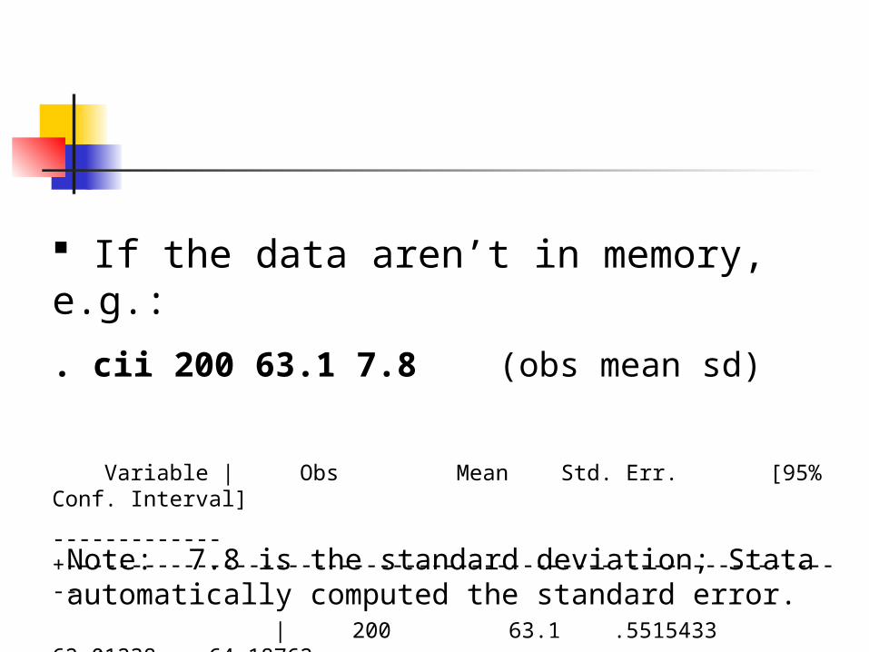
If the data aren’t in memory, e.g.:

. cii 200 63.1 7.8 (obs mean sd)

Variable | Obs Mean Std. Err. [95% Conf. Interval]

-------------+-------------------------------------------------------------

| 200 63.1 .5515433 62.01238 64.18762

Note: 7.8 is the standard deviation; Stata automatically computed the standard error.

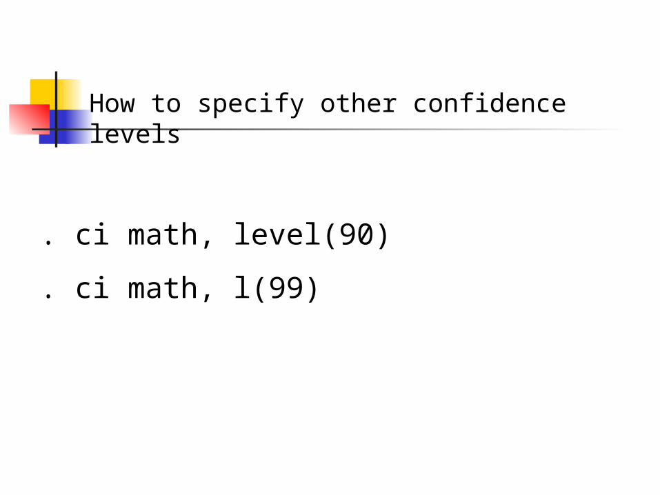
. ci math, level(90)

. ci math, l(99)

How to specify other confidence levels

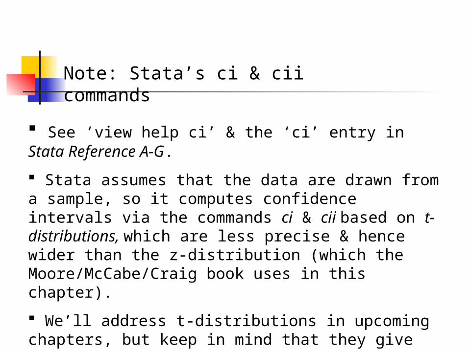
Note: Stata’s ci & cii commands

See ‘view help ci’ & the ‘ci’ entry in Stata Reference A-G.

Stata assumes that the data are drawn from a sample, so it computes confidence intervals via the commands ci & cii based on t-distributions, which are less precise & hence wider than the z-distribution (which the Moore/McCabe/Craig book uses in this chapter).

We’ll address t-distributions in upcoming chapters, but keep in mind that they give wider CI’s than does the z-distribution.

Confidence intervals, & inferential statistics in general, are premised on random sampling or randomized assignment & the long-run laws of probability.

A confidence interval is a range that captures the ‘true value’ of a statistic with a specified probability over repeated random sampling of the same size in the same population.

Review: Confidence Intervals

If there’s no random sample or randomized assignment (or at least independent observations, such as weighing oneself repeatedly over a period of time), the use of a confidence interval is invalid.

What if you have data for an entire population? Then there’s no need for a confidence interval: terrific!

Example: Is there a statistically significant difference in the average size of our solar system’s gas and non-gas planets?

Source: Freedman et al., Statistics.

Example: 27% of the female applicants to a graduate program gain admission, while 24% of the male applicants do.

Is this a statistically significant difference?

See Freedman et al.

The sample’s confidence interval either captures the parameter or it doesn’t: it’s an either/or matter.

We’re saying that we calculated the numbers according to a method that, according to the laws of probability, will capture the parameter in [90% or 95% or 99%] of all possible random samples of the same size in this population.”

That means, though, that in a certain percent of samples (typically 5%) the confidence interval does not capture the parameter.

And we don’t know when it doesn’t capture the parameter.

There are two sources of uncertainty: probabilistic (sampling) & non-probabilistic (non-sampling).

Reasons to review Chapter 3

All conclusions are uncertain.

How to reduce a confidence interval’s margin of error?

Use a higher level of confidence (e.g., from 95% to 99%) to widen the confidence interval (which is the least recommended of the options)

Increase the sample size (much larger n; four times larger to reduce the CI by one half).

Reduce the standard error (via more precise measurement of variables &/or more precise sample design).

What is significance testing?

How do confidence intervals pertain to significance testing?

Significance Tests

Variability is everywhere.

“… variation itself is nature’s only irreducible essence.” Stephen Jay Gould

E.g., weighing the same item repeatedly.

E.g., measuring blood pressure, cholesterol, estrogen, or testosterone levels at any various times.

E.g., performance on standardized tests or in sports events at various times.

In short, the objective of a test for statistical significance is to identify a durable relationship in a mosaic of chance variation.

For any given unbiased measurement:

sample measured value = true value +/- random error

How do we statistically distinguish an outcome potentially worth paying attention to from an outcome based on mere random variability?

That is, how do we distinguish a an outcome potentially worth paying attention to from an outcome based on mere chance?

We do so by using probability to establish that a sampled magnitude (of effect or difference) would rarely occur by chance.

The scientific method tries to make it hard to establish that such an outcome occurred for reasons other than chance.

It makes us start out by asserting a null hypothesis: a claim about a population that we must attempt to contradict by means of a sample’s evidence.

Hence significance tests, like confidence intervals, are premised on a variable’s sampling distribution.

I.e., they are premised on what would happen with repeated random samples of the same size in the same population, independently carried out over the very long run.

The null hypothesis is the starting point for a significance test: it is an assertion about a population or relationship within a population that we test.

It asserts the following about the parameter: zero; no effect; untrue; or equals some benchmark value.

Significance Tests: Stating Hypotheses

That is, a null hypothesis states the opposite of what we want to find.

E.g., does not equal zero; is greater than zero; there is an effect; is different from the benchmark value.

For example, what would be a null hypothesis concerning residential proximity of power lines & rate of cancer for a population?

The alternative hypothesis contradicts the null hypothesis. It states what we want to find.

The alternative hypothesis claims that the parameter’s value is significantly different from that of the null hypothesis.

That is, it claims that the alternative value is large enough that it would rarely have occurred in a sample by chance.

What would be an alternative hypothesis for the power line/ cancer study?

The statement being tested in a significance test is the null hypothesis.

We examine a sample’s evidence against the null hypothesis: does the sample’s evidence permit us to reject the null hypothesis?

So, we examine a sample’s evidence against the null hypothesis from the standpoint of an alternative hypothesis.

The significance test is designed to assess the strength of the sample’s evidence against the null hypothesis.

It does so in terms of the alternative hypothesis.

The alternative hypothesis may be one-sided or two-sided.

A one-sided example for the power line/cancer study? A two-sided example?

Is the magnitude of the sampled, alternative value large enough relative to its standard error to have rarely occurred by chance?

I.e., if there really is no effect, then would it be rare for a sample to have detected an effect of this magnitude or greater?

The Basic Hypothesis-Testing Question

Hypotheses always refer to some population (i.e. to a parameter of individuals or processes), not to a sample.

That is, hypotheses always infer from a sample to a population: what are the chances of observing the sampled value (as specified in the alternative hypothesis) if this sample were repeated again & again?

Tests of Population or Model

A statistical hypothesis, then, is a claim about a population (of individuals or processes, including a relationship within a population).

Therefore always state a hypothesis in terms of a population.

Examples?

Does the sample’s evidence contradict the null hypothesis, or not?

Depending on the test results, we either fail to reject the null hypothesis or reject the null hypothesis.

We never accept the null hypothesis (or the alternative hypothesis)—why not?

As Halcousis (Understanding Econometrics, page 44) puts it:

“If you can reject a null hypothesis, it is likely that it is false.” Why?

“If you cannot reject a null hypothesis, think of the test as inconclusive.” Why?

Let’s explore what these statements mean.

Statistical significance means that if the null hypothesis were true (i.e. if there really were no effect), then the magnitude of the sampled effect would be likely to occur by chance in no more than some specified percentage (typically 5%) of samples.

What does statistical significance mean?

Test Statistic

A test statistic assesses the null hypothesis in terms of the sample’s data.

It is computed as a z-value (or, as we’ll see for random samples, a t-value).

Dividing by the standard error reflects the fact that the data are drawn from a sample.

How to compute the test statistic

sample-observed mean minus hypothesized mean

divide by the standard error to find the test statistic

Where does the test statistic (z-value or t-value) anchor the finding on the normal distribution? What is the probability associated with the test statistic’s location on the normal distribution?

Logic of the Hypothesis Test

Ratio of the sampled magnitude of effect to the standard error (i.e. random variation).

The larger the ratio, the less likely that the sampled magnitude of effect was due to chance (i.e. to sampling error [random variation]).

Based on our conceptualization of a research question, we formulate a null hypothesis & an alternative hypothesis:

. Ho: = …

. Ha: < ~= > …

After confirming that the sample is random and of acceptable size and perhaps that the Central Limit Theorem holds, we test the hypothesis.

How to test a hypothesis

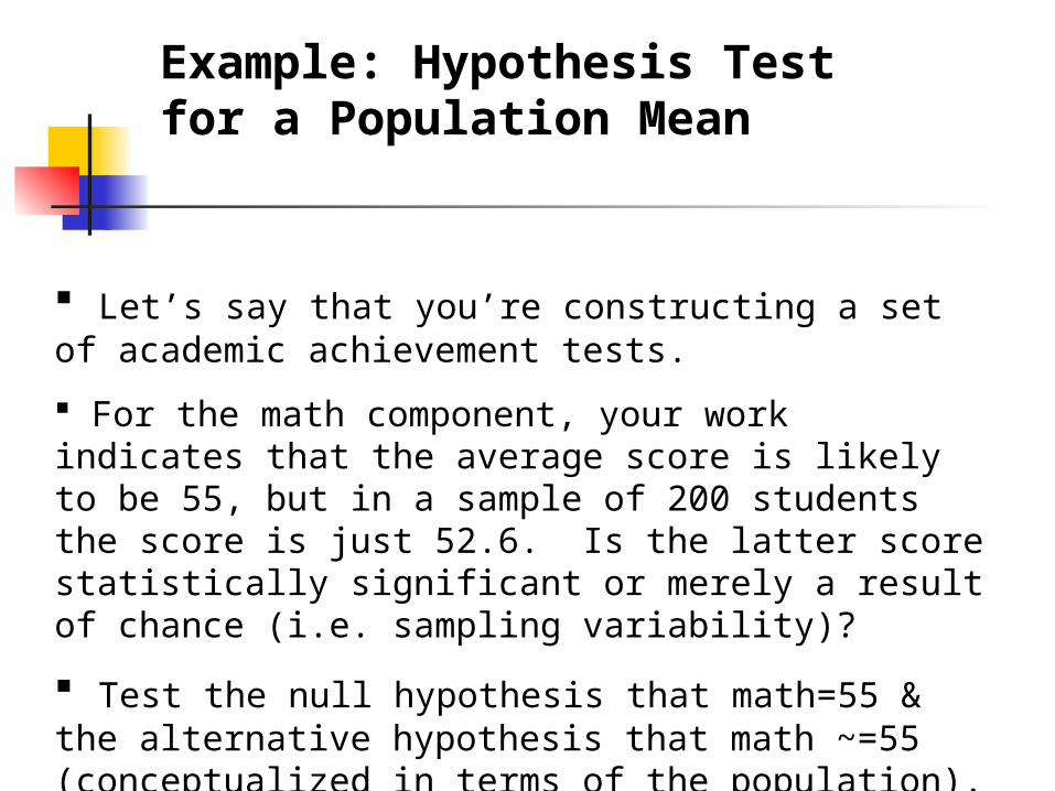
Let’s say that you’re constructing a set of academic achievement tests.

For the math component, your work indicates that the average score is likely to be 55, but in a sample of 200 students the score is just 52.6. Is the latter score statistically significant or merely a result of chance (i.e. sampling variability)?

Test the null hypothesis that math=55 & the alternative hypothesis that math ~=55 (conceptualized in terms of the population).

Example: Hypothesis Test for a Population Mean

0.0

1.0

2.0

3.0

4D

en

sity

30 40 50 60 70 80math score

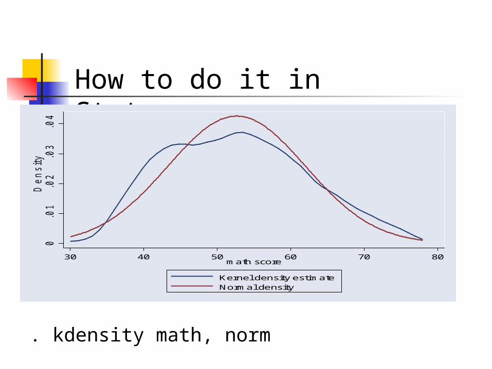
Kernel density estimateNormal density

. kdensity math, norm

30

40

50

60

70

80

math

score

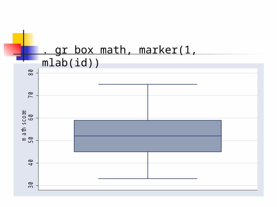
. gr box math, marker(1, mlab(id))

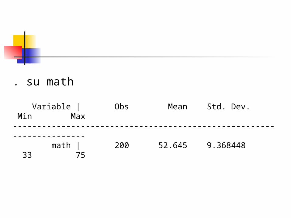
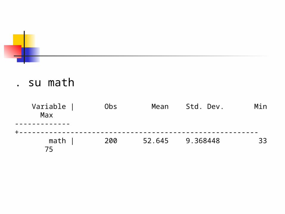
. su math

Variable | Obs Mean Std. Dev. Min Max--------------------------------------------------------------------- math | 200 52.645 9.368448 33 75

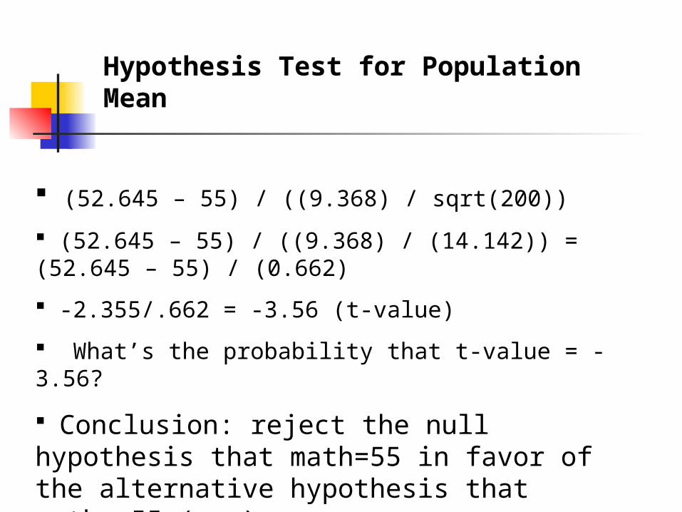
(52.645 – 55) / ((9.368) / sqrt(200))

(52.645 – 55) / ((9.368) / (14.142)) = (52.645 – 55) / (0.662)

-2.355/.662 = -3.56 (t-value)

What’s the probability that t-value = -3.56?

Conclusion: reject the null hypothesis that math=55 in favor of the alternative hypothesis that math~=55 (p=…).

Hypothesis Test for Population Mean

Logic of the Hypothesis Test

Magnitude of the difference between the sampled value & the hypothesized value in relation to the standard error (i.e. sampling variability [random variation]).

I.e., the ratio of the sampled value’s size to the standard error’s size.

The bigger the ratio, the bigger the z- or t-value & hence the lower the P-value: the less likely that the finding is due to chance (i.e. sampling variability [random variation]).

Note: Stata’s ttest & ci

ttest and ci yield wider confidence intervals than does the z-value formula given in this chapter by Moore/McCabe.

Stata’s ttest and ci are based on t-distributions, but Moore/McCabe/ Craig’s formula in this chapter is based on the z-distribution.

Statistical Significance: P-value

P-value (probability value) of the test: the probability that the test statistic would be as extreme or more extreme than its sampled value if the null hypothesis were true (i.e. if there really were no effect).

The P-value is the observed (i.e. sampled) level of statistical significance.

The P-value expresses the probability of finding the sampled effect in terms of the standard normal distribution of sample means.

A P-value is the probability that the sample incorrectly rejected the null hypothesis.

I.e., it’s the probability that a sample would detect the observed magnitude if there really were no effect.

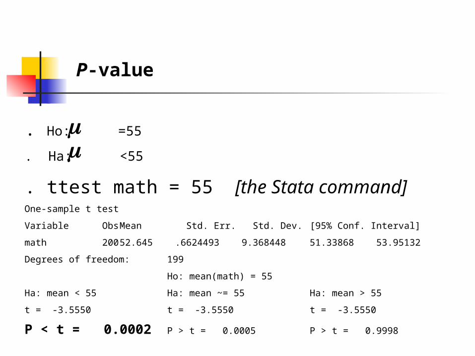
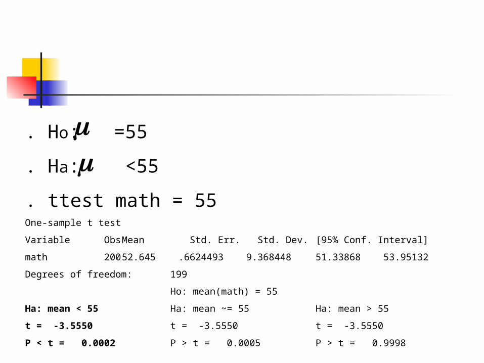
. Ho: =55

. Ha: <55

. ttest math = 55 [the Stata command]One-sample t test

Variable Obs Mean Std. Err. Std. Dev. [95% Conf. Interval]

math 200 52.645 .6624493 9.368448 51.33868 53.95132

Degrees of freedom: 199

Ho: mean(math) = 55

Ha: mean < 55 Ha: mean ~= 55 Ha: mean > 55

t = -3.5550 t = -3.5550 t = -3.5550

P < t = 0.0002 P > t = 0.0005 P > t = 0.9998

P-value

The smaller the P-value, the stronger the data’s evidence against the null hypothesis.

That is, the smaller the P-value, the stronger the data’s evidence in favor of the alternative hypothesis. Why?

The P-value is small enough to be statistically significant if the magnitude of the sampled effect is sufficiently large in relation to its standard error (i.e. sampling error [random variation]).

The P-value, to repeat, is the observed significance level.

The P-value is based on the sampling variability of the sample mean.

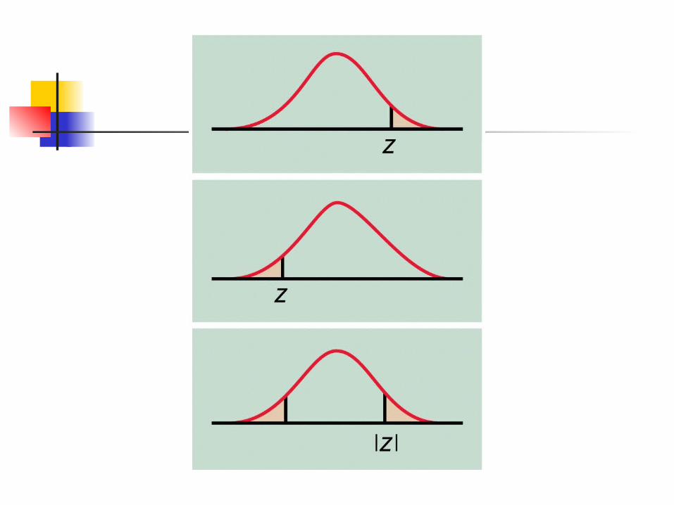
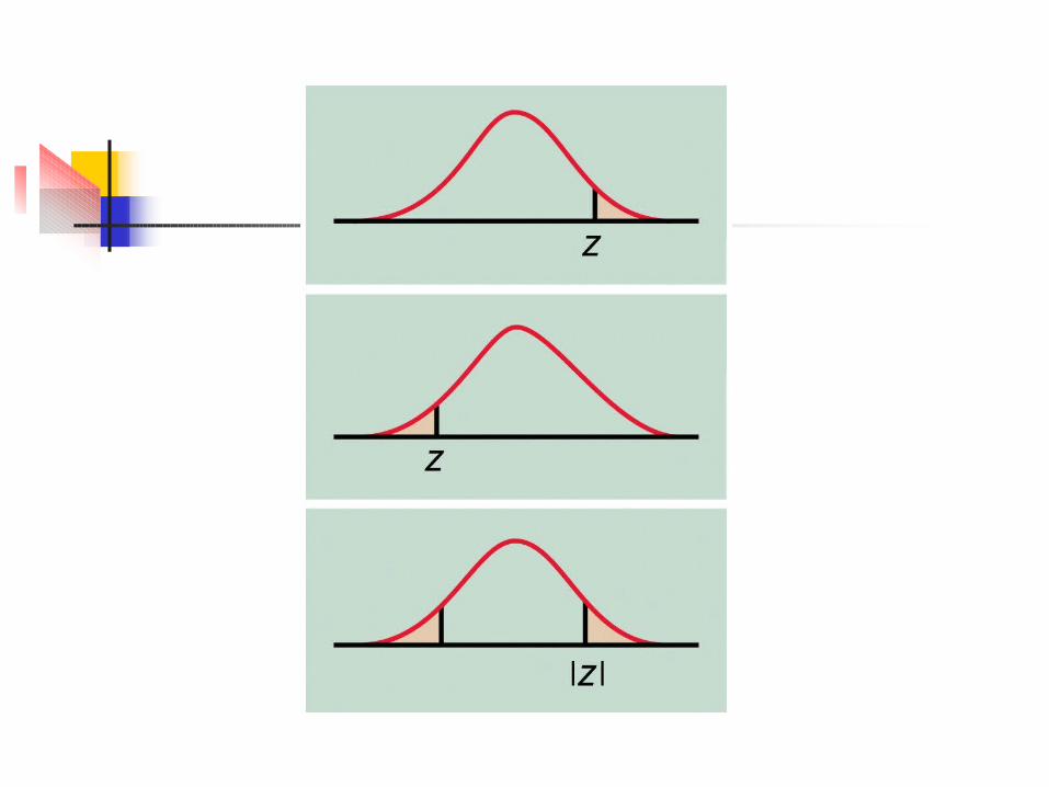
Depending on the form of the alternative hypothesis, the significance test may be one-tailed or two-tailed.

One- or two-tailed significance tests

If the P-value is as small or smaller than a specified significance level (conventionally .10 or .05 or .01), we say that the data are statistically significant (at p=…., for a one-tailed or two-tailed test, df=…).

Statistical significance means that if the null hypothesis were true (i.e. if there really were no effect), then a finding of the sampled effect or stronger would occur by chance in no more than some specified percentage (typically 5%) of samples.

To repeat:

A P-value, then, is the probability that the sampled value leads you to incorrectly reject a null hypothesis.

How to do it in Stata0

.01

.02

.03

.04

Den

sity

30 40 50 60 70 80math score

Kernel density estimateNormal density

. kdensity math, norm

30

40

50

60

70

80

math

score

. gr box math, marker(1, mlab(id))

. su math

Variable | Obs Mean Std. Dev. Min Max-------------+-------------------------------------------------------- math | 200 52.645 9.368448 33 75

. Ho: =55

. Ha: <55

. ttest math = 55 One-sample t test

Variable Obs Mean Std. Err. Std. Dev. [95% Conf. Interval]

math 200 52.645 .6624493 9.368448 51.33868 53.95132

Degrees of freedom: 199

Ho: mean(math) = 55

Ha: mean < 55 Ha: mean ~= 55 Ha: mean > 55

t = -3.5550 t = -3.5550 t = -3.5550

P < t = 0.0002 P > t = 0.0005 P > t = 0.9998

Reject the null hypothesis in favor of the alternative hypothesis (p=.000, one-tailed test, df=199).

Note: for a one-tailed test, if the observed effect is not in the hypothesized direction then there is no evidence to reject the null hypothesis.

Two-tailed tests are the mainstay: they provide a more conservative test (i.e. it’s harder to obtain significance with a two-tailed test) & they’re virtually always considered to be appropriate.

As the next slide shows…

How to obtain a one-tailed test from a two-tailed test: P-value/2.

How to obtain a two-tailed test from a one-tailed test: P-value*2.

To show that it’s easier to obtain significance in a one-tailed test:

. two-tailed test: p-value=.08

. one-tailed test: .08/2=.04

Statistical significance does not mean theoretical, substantive or practical significance.

In fact, statistical significance may accompany a trivial substantive or practical finding.

What Statistical Significance Isn’t, & What It Is

Depending on the test results, either we fail to reject the null hypothesis or we reject the null hypothesis.

We never accept the null hypothesis (or the alternative hypothesis): Why not?

Regarding statistical significance, it’s useful to think (more or less) in terms of the following scale:

p<.10: some statistical significance

p<.05: moderate statistical significance

<.01: strong statistical significance

<.001: very strong statistical significance

Approximate Interpretations

Engineers: the standard is p<.01

Medicine: the standard is p<.05

Social sciences: the standard is p<.05.

Nevertheless …

These levels (called critical values, which include each value’s critical region of more extreme values) are cultural conventions in statistics & research methods.

There’s really no rigid line between statistical significance & lack of such significance, or between any of the critical levels of significance.

Listing the P-value provides a more precise statement of the evidence.

E.g.: the evidence fails to reject the null hypothesis at any conventional level (p=.142, two-tailed test, df=199).

Let’s remember, moreover: statistical significance does not mean theoretical, substantive, or practical significance.

In any event, statistical significance—as conventionally defined—is much easier to obtain in a large sample than a small sample.

Why?

Because according to the formula, a sample statistic’s standard error decreases as the sample size increases.

A large enough sampled effect relative to the standard error.

A large enough sample size to minimize the role of chance in determining the finding.

What does it take to obtain statistical significance?

Consequently, lack of statistical significance may simply mean that the sample size is not large enough to override the role of chance in determining the finding.

It might also mean that the variables in question are inadequately constructed (i.e. inadequately measured).

It further could mean that the relationship is non-linear, so appropriate transformations may be called for.

Or it could be that the sample is badly designed or executed, that there are data errors, or that there are other problems with the study.

Of course, it may indeed mean that the hypothesized value or effect simply isn’t large enough to minimize the role of chance in causing the observed finding.

Statistical significance does not necessarily mean substantive or practical significance.

Statistical significance may, in any case, be an artifact of chance (i.e. the 5% samples that got the parameter wrong), which is especially likely to occur in large samples.

And remember: significance tests are premised on a random sample or randomized assignment, or at least independent, representative observations.

Statistical significance tests are invalid if the sample cannot be reasonably defended as (1) random, (2) a randomized experiment, or (3) at least consisting of independent, representative observations; or if measurements are obtained for an entire population (the latter being a good thing, however).

Without random sampling or random assignment (or at least, independent, representative observations as when weighing an object repeatedly over a period time), the laws of probability can’t operate.

With measurements on an entire population, there is no sampling-based uncertainty to test (or worry about).

The two-sided hypothesis test can be directly computed from the confidence interval.

CI’s & two-sided hypothesis tests

For a two-sided hypothesis test of a population mean, if the hypothesized value falls outside the confidence interval, then we reject the null hypothesis.

Why?

Because it’s quite unlikely (say, p<.05) that the hypothesized value characterizes the population.

That is, it’s quite unlikely that the sampled captured the observed value by chance.

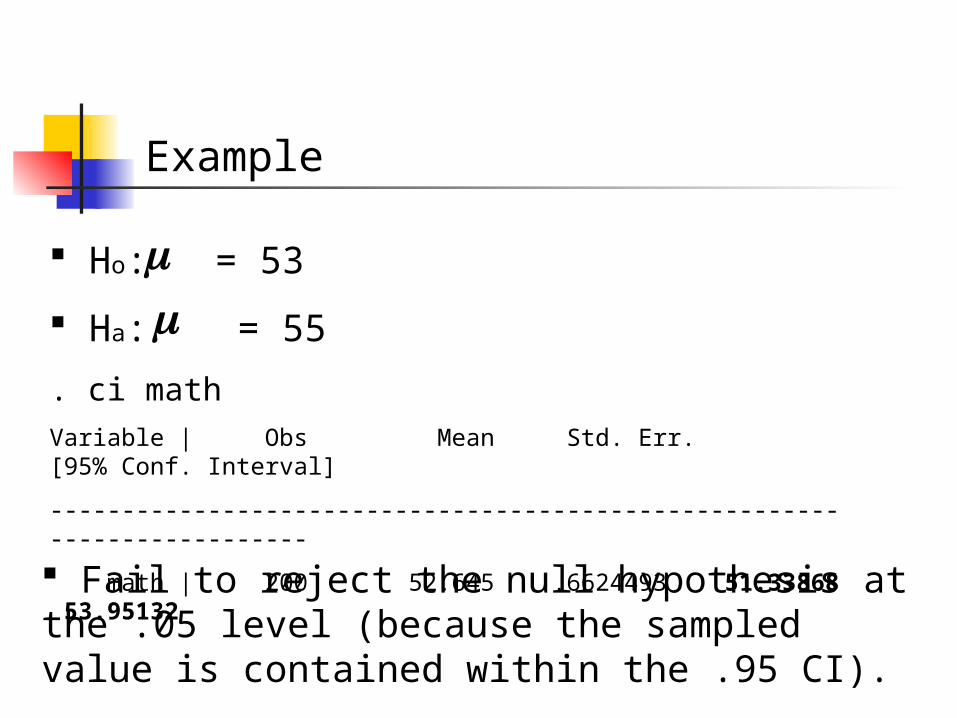
Ho: = 53

Ha: = 55

. ci mathVariable | Obs Mean Std. Err. [95% Conf. Interval]

-------------------------------------------------------------------------

math | 200 52.645 .6624493 51.33868 53.95132

Example

Fail to reject the null hypothesis at the .05 level (because the sampled value is contained within the .95 CI).

Review: Significance Testing

Significance testing is premised on a random sample of independent observations, randomized assignment, or, minimally, independent , representative observations: if this premise does not hold, then the significance tests are invalid.

Statistical significance does not mean theoretical, substantive or practical significance.

Statistical significance means that an effect as extreme or more extreme in a random sample of independent observations is unlikely to have occurred by chance in more than some specified percentage (typically 5%) of samples.

It is the probability that this happened in the sample if there really were no effect in the population.

Any finding of statistical significance may be an artifact of large sample size.

Any finding of statistical insignificance may be an artifact of small sample size.

Moreover, statistical significance or insignificance in any case may be an artifact of chance.

What does a significance test mean?

What does a significance test not mean?

What is the procedure for conducting a significance test?

What is the P-value?

Why is the P-value preferable to a fixed significance level?

What are the possible reasons why a finding does not attain statistical significance?

What are the possible reasons why findings are statistically significant?

Depending on the test results, we either fail to reject the null hypothesis or reject the null hypothesis.

We never accept the null hypothesis (or the alternative hypothesis).

Beware!

There is no sharp border between ‘significant’ & ‘insignificant’, only increasingly strong evidence as the P-value gets smaller.

There is no intrinsic reason why the conventional standards of statistical significance must be .10 or .05 or .01 (or .001).

Don’t ignore lack of statistical significance: it may yield important insights (such as failure to find female-male differences).

Beware of searching for significance: by chance alone, a certain percentage of findings will indeed attain statistical significance.

There’s always uncertainty in assessing statistical significance.

If a finding tests significant, the null hypothesis may be wrongly rejected: Type I error.

If a finding tests insignificant, the null hypothesis may be wrongly ‘accepted’: Type II error.

Another Problem: Two Types of Error in Significance Tests

Type I error: e.g., a ‘false positive’ medical test – a test erroneously detects cancer.

Type II error: e.g., a ‘false negative’ medical test – a test erroneously does not detect cancer.

A P-value is the probability of a Type I error.

Increasing a test’s sensitivity (ability to detect Ha when it is ‘true’) reduces the chance of Type I error: e.g., making a test more sensitive to detecting cancer by increasing its critical value from .05 to .10

We have to decide in any given test: Are we more worried about a false positive (Type I error) or a false negative (Type II error).

What are the practical concerns?

The difficult choice: protecting more against one makes the test more vulnerable to the other.

Examples: tests for cancer; airport detection devices; or that auto brake component may fail.

In these examples, do we typically seek to minimize Type I error or Type II error, & why?

Power: measured as a test’s ability reject the null hypothesis when a particular value of the alternative hypothesis is true.

E.g., if the district’s current SAT mean=500, what will be the power of the test to detect a 10-point increase at p=.05?

Power = 1 – prob. of Type II error

We want high power, .80 (i.e. 80%), so that prob. Type II error<=.20 (i.e. 20%).

See the example in Moore/McCabe.

How to increase power?

Increase the sample size

Reduce variability: either sample a more homogeneous population, sample more precisely, or otherwise improve measurement precision

Increase the critical value (e.g. from .05 to .10).

Specify that the test criterion’s value is farther away from Ho (say, 20 points instead of 10 points), because larger differences are easier to detect.

Type I/II Errors & Power in Stata

See Stata ‘help’ &/or the documentation manual for the command ‘sampsi.’

Bonferroni adjustment

When there are multiple hypothesis tests, the Bonferroni adjustment makes it tougher to obtain statistical significance: What’s the reason for doing so?

Divide the selected critical value (such as p<.05) by the number of hypothesis tests.

Selected critical level: p<.05

Five tests

.05/5=.01

Thus, each test will be judged as statistically significant only at p<.01 or less.

There are other ‘multiple adjustments’ tests, such as Scheffe, Sidak, & Tukey.

In Stata, specify, e.g., the subcommand bonf or sch or sid, according to the particular procedure.

Review Again

What’s a null hypothesis?

What’s an alternative hypothesis?

What specifically do we test?

How do we state our conclusions for an hypothesis test?

Why do we never ‘accept’ a null hypothesis or alternative hypothesis?

What’s the premise of significance tests? What if the premise doesn’t hold?

What is the procedure for conducting a significance test?

What do significance tests mean? What don’t they mean?

What conditions yield a statistically significant finding? What conditions don’t yield such a finding?

What is a P-value?

Why is a P-value preferable to a fixed significance level?

Why are .10, .05 & .01 so commonly used as critical values?

How should we treat statistically insignificant findings?

Why shouldn’t we search for statistical significance?

Why is a finding of statistical significance uncertain? Why is a finding of statistical insignificance uncertain?

What are Type I errors? What is the the statistic that represents the probability of a Type I error?

What are Type II errors?

What’s a Bonferroni adjustment (or other ‘multiple adjustment’)?

Why is it used?

For what various reasons are conclusions inherently uncertain?

Significance Testing: Questions

True or false, & explain:

A difference that is highly significant statistically must be very important.

Big samples are bad.

Source of the questions: Freedman et al., Statistics.

If the null hypothesis is rejected, the difference isn’t trivial. It is bigger than what would occur by chance, correct?

For one year in one graduate major at a university, 825 men applied & 62% were admitted; 108 women applied & 82% were admitted. Is the difference statistically significant?

Questions continued…

The masses of the inner planets average 0.43 versus 74.0 for the outer planets. Is the difference statistically significant? Does this question make sense?

A P-value of .047 means something quite different from one of .052. Right?

Questions continued…

According to the U.S. Census, in 1950 13.4% of the U.S. population lived in the West; in 1990 21.2% lived in the West. Is the difference statistically significant? Practically significant?

Questions continued…

Morals of the Stories

Statistical significant says nothing about: practical significance

the adequacy of the study’s design/measurement

whether or not the study is based on a random sample, randomized assignment, or at least independent, representative observations.

Professional standards of statistical significance are cultural conventions: there’s no intrinsic, hard line between statistical significance & insignificance.

Findings of statistical insignificance may be more insightful than those of statistical significance.

Finally, confidence intervals & significance tests are based on a random variable’s sampling distribution: over all possible random samples (or randomized assignments, or independent, representative observations) of the same size in the same population.

See the class document ‘Graphing confidence intervals in Stata’.