الرحيم الرحمن الله بسم

Signals and SystemsLecture 15: Laplace Transform

University of Khartoum

Department of Electrical and Electronic Engineering

Third Year - 2015

Dr. Iman AbuelMaaly Abdelrahman

Outline

• Signal Transforms• Laplace Transform• Region of Convergence• Pole-Zero Plot• Exercises

2 2015

Signals Transform

Continuous-Time signals Discrete-Time signals

Signal in time domain x(t)

Signal in frequency domain - Fourier Series Ck

- Fourier Transform X(jω)

Signal in Laplace domai - - - Laplace Transform X(s)

Signal in time domain x[n]

Signal in frequency domain - Fourier Series Ck

- Fourier Transform X(ejω)

Signal in Z- domain- Z- Transform X(Z)

3

DSP

DSP

The Laplace Transform

• Assume s is any complex number of form:s = + j

• That is, s is not purely imaginary and it can also have real values.

• X(s)|s=j=X(j).

• X(s) is called the Laplace transform of x(t)

)()( sXtx L4 2015

In general, for a signal x(t):

Is the bilateral Laplace transform, and

Is the unilateral Laplace transform.

dtetxsX st)()(

0

)()( dtetxsX st

Laplace Transform

5

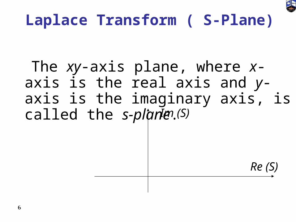
The xy-axis plane, where x-axis is the real axis and y-axis is the imaginary axis, is called the s-plane.

Laplace Transform ( S-Plane)

Re (S)

Im (S)

6

• Fourier transform is the projection of Laplace transform on the imaginary axis on the s-plane.

• This gives two additional flexibility issues to the Laplace transform:–Analyzing transient behavior of systems–Analyzing unstable systems

Laplace Transform

7

Region of Convergence (ROC)

• Similar to the integral in Fourier transform, the integral in Laplace transform may also not converge for some values of s.

• So, Laplace transform of a function is always defined by two entities:–Algebraic expression of X(s).–Range of s values where X(s) is valid, i.e.

region of convergence (ROC).

8 2015

Region of Convergence (ROC)

The ROC consists of those values of

for which the Fourier Transform of

Converges

js

tetx )(

9 2015

•Transform techniques are an important tool in the analysis of signals and LTI

systems .•The Z-transform plays the same role in the

analysis of discrete-time signals and LTI systems as the Laplace transform does in the analysis of continuous-time signals and systems.

The Laplace Transform

10

Example (L-Transform)

Compute the Laplace Transform of the following signal:

For what values of a X(s) is valid?

)()( tuetx at

11 2015

Obtain the Fourier Transform of the signal

dtetxjX tj )()(

(1)12

• Laplace Transform

or with

dteejX tjta )()(

dtetuedtetxsX statst )()()(

js

13 2015

By comparison with Eqn )1( we recognized Eqn)1( as the Fourier Transform of

And Thus,

)()( tue ta

0,)(

1)(

a

jajX

14 2015

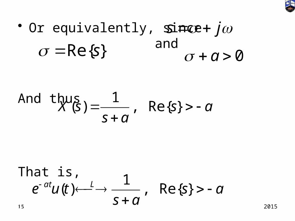
• Or equivalently, since and

And thus

That is,

js }Re{s

asas

sX

}Re{,1

)(

asas

tue Lat

}Re{,1

)(15

0 a

2015

16 2015

Example 2

)()( tuetx at

0)(

)()(

dte

dttueesX

tas

stat

asas

tue Lat

}Re{,1

)(17 2015

t

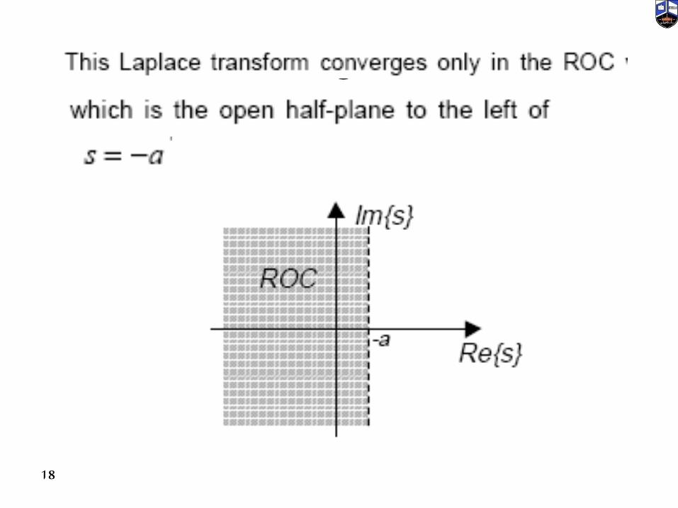
18

19

20

21 2015

Pole-Zero Plot

• Given a Laplace transform

- Poles of X)s(: are the roots of D)s(.

- Zeros of X)s(: are the roots of N)s(.

22

)(

)()(

sD

sNsX

2015

Example3 Find X(s) for the following x(t).

)(2)(3)( 2 tuetuetx tt

23

1}Re{,1

1)(

2}Re{,2

1)(2

ss

tue

ss

tue

Lt

Lt

2015

• The set of values of Re{s} for which the Laplace transforms of both terms converges is Re{s} >-1, and thus combining the two terms on the right hand side of the above equation we obtain:

1}Re{,23

1)(2)(3

22

sss

stuetue Ltt

24

1}Re{,1

2

2

3)(

s

sssX

2015

Has poles at p1 =-1 and p2 =-2 and a zero at z =1

25

1}Re{,)1)(2(

1)(

s

ss

ssX

2015

Re

Im

-1-21

XX

zerospole

S-planeROC

26

1}Re{,)1)(2(

1)(

s

ss

ssX

Inverse Laplace Transform

• Integral of inverse Laplace transform:

• However, we will mainly use tables and properties of Laplace transform in order to evaluate x)t( from X)s(.

• That will frequently require partial fractioning.

j

j

stdsesXj

tx )(2

1)(

27

Laplace Transform and LTI

In the above system, H)s( is called the transfer function of the system. It is also known as Laplace transform of the impulse response h)t(.

)()(

)()( )(

sHedehe

dehty

stsst

ts

LTI

x(t)=est y(t)=h(t)* est

28 2015

System Characterization by LT

Causality

Stability

h(t)x(t) y(t)

29

)()()()()()( sHsXsYthtxty L

30