1.

Learning Objectives: 3f) Embedded Options: Complete analysis that may include calculation of hedging cost,

deterministic and stochastic analysis of cash flow, reserves, and capital levels under a range of economic environments

This question asks the candidate to assess different risks in a portfolio and make appropriate modifications. Part (b) relates the portfolio’s dynamics to the actuarial models. ALM actuaries frequently work on such projects. The solution is primarily based on Babbel & Fabozzi chapters 19 and 21, but integrates knowledge of asset class behavior from the Fabozzi text.

Solution: (a) Sources of risk

1. Interest rate risk • Callable corporate bonds (CCB) - prices increase as interest rates decrease,

although the call option dampens this effect • Mortgage pass-through securities (MBS) - prices decrease as interest rates

increase in a similar manner to the price behavior of comparable Treasury Securities

2. Credit risk (Spread risk, default risk)

• CCB - spreads can change in relation to comparable Treasury securities vs. those embedded in the purchase price

• MBS - spreads can change in relation to Treasury securities based on the market's valuation of the homeowners' prepayment option

• The source of this risk is the market's valuation of the risk inherent in the

underlying issuer's default risk in the case of CCB, and in the homeowner's default risk in the case of MBS. In addition, for MBS, the spread risk incorporates the valuation of the homeowner's pre-payment option.

3. Prepayment risk

• MBS - the risk that homeowners of the underlying mortgages will pre-pay them as interest rates decline, leaving funds to reinvest at lower rates than those that were available at the time of purchase of the MBS.

• This gives rise to negative convexity, because the percentage increase in the

prices of MBS gets smaller for each successive decrease in interest rates,

1. and the percentage decrease in the prices of MBS gets larger for each successive increase in interest rates.

• For CCB, this is similar to the issuer exercising the call option before maturity.

4. Volatility risk

• MBS - the spreads of MBS in relation to Treasuries will increase as the expected future interest rate volatility increases, while these spreads will decrease as the expected future interest rate volatility decreases.

5. Model risk

• MBS - the risk that the model will fail to accurately predict the prepayment behavior of the security.

(b)

1. Effects of gradual decreases in long-term interest rates

• CCB - value of call option increases, limiting the price increases that would otherwise have occurred if the bond were non-callable. Although sales of bonds could result in capital gains, the proceeds can only be reinvested at lower rates

• MBS - pre-payments will increase as interest rates decline, and the cash flows

will have to be reinvested at lower rates than the minimum guaranteed interest rate for the Non-Traditional liabilities

2. Effects of rising rate scenarios:

• CCB - value of call option decreases, which increases the price of the bond, while increasing duration. Sales could be at lower prices than par, resulting in capital losses, while attempting to fund the liability payments.

• MBS - the prepayment activity slows, resulting in reduced cash flow to fund

liability payments (c) Strategy

• Purchase more MBS, in order to lower the effective duration of assets to better match that for the liabilities. Consider MBS issued by Government Sponsored entities, in order to limit default risk. Fund the purchase of MBS through the sale of government bonds, which will result in the sale of a high duration asset and substitution of a lower duration asset.

2. Learning Objectives: 3e) Portfolio Rebalancing: Identify investment strategies that do not currently achieve

portfolio management objectives and recommend appropriate changes. Improved strategies may include shifts in asset allocation, use of swaps, forwards, and futures, and use of options

This question asks the candidate to evaluate a particular case study portfolio and recommend an approach to improve it, a realistic situation for an investment actuary. No derivatives are involved. The solution is based on Maginn & Tuttle chapter 11 and knowledge of asset class behavior from Fabozzi.

Solution: a) Buy and hold means you buy the asset and hold the asset until maturity. This strategy

will outperform with markets are consistently up or down. It is neutral when markets are flat.

Constant mix means you hold assets according to a target weight of the portfolio. When markets are consistently up or down, it will underperform, when markets are flat, it will outperform. Equity allocation is a fixed percentage of portfolio. It represents the sale of portfolio insurance. Constant proportion means you hold each asset according to a percentage of a cushion value (portfolio value – floor value). When stock prices go up, you buy, when prices go down, you sell. It will underperform when the market is flat, and will outperform when markets are consistently up or down. It represents the purchase of portfolio insurance. b) Buy and hold is a linear function of stock returns. Portfolio return is a linear function

of stock returns. Constant mix is a concave function of stock returns. Portfolio return increases at a decreasing rate when stock return is positive and decreases at an increasing rate when returns are negative. Constant proportion is a convex function of stock returns. Portfolio return increases at an increasing rate when returns are positive and decreases at a decreasing rate when returns are negative. c) Want to maximize total return of Surplus Account over time subject to some

constraints. Current target mix is 50% equities, 35% real estate, and 15% bonds. In my opinion, the company should use Constant Proportion since this gives the Surplus Account a guaranteed value (floor value). It performs better when markets are up. Constant mix doesn’t address downside risk.

3. Learning Objectives: 3b) Incorporate the parameters affecting the client’s needs in an asset-liability

management framework including: funding objectives, risk/return tradeoffs, regulatory and rating agency requirements, concerns about solvency, capital, tax and accounting considerations, and management constraints.

This question asks the candidate to look at a life insurer’s ALM and liquidity risk from an outsider’s perspective – that of a rating agency. Investment actuaries are frequently called upon to prepare material or present to rating agency analysts. The solution requires familiarity with Tillman chapter 13.

Solution: a) Explain how the typical rating agency examines ALM and liquidity exposure for

the purpose of assigning a rating.

• General methodology involves a qualitative assessment of the techniques management uses to ensure its assets are adequate to meet potential short and long term liability needs.

• Analysis takes a comprehensive view of ALM, looking at how all risks are accounted for to ensure a prudent investment approach

• Looks at typical interest rate risk and product secondary guarantees, as well as other liability features, e.g. book value cashout option

• Agency will look at duration matching techniques, key rate duration exposure, dynamic CF testing focusing on a variety of economic scenarios and their impact on the company’s earnings and capital

• Also need to take a detailed look at embedded options in liabilities (leading to need for liquidity), what are management’s plans in time of crisis, what is the nature of the assets backing the liabs.

b) Describe how the typical rating agency assesses the key ALM and liquidity issues

associated with institutional investment products.

• These products are guaranteed investment contracts (GICs) and funding arrangements and have ALM issues similar to retail fixed annuities.

• The key ALM issue relates to the “lumpiness” of this business, where a single transaction is generally significant in size in relation to a single retail fixed annuity (liquidity).

3. • Liquidity is a major concern if the client leaves the insurer, often at the worst

possible time – where does the money come from? • Will the insurer take losses by liquidating investments early in a down market

(or higher yield environment) • Rating agencies believe a carrier has only limited capacity to issue this

business as a result and considers any more than 20-30% of this business in relation to the total company general account business to be high

• Various risk weight factors have been developed to appropriately measure the risk this business brings to a company (quick ratio, capacity limits)

• Ability to assign or already assigned collateral and C3 required capital are indicators of prudent management

c) Calculate and interpret the following two tests of LifeCo’s Institutional

Pensions-GIC disintermediation risk. Assume that Mud & Poor’s used 1 / duration (in years) as a measure to approximate the annual amount of maturities, and that NAIC 1 plus NAIC 2 bonds correspond to government and public investment grade bonds.

i) Capacity limit ii) Insurance quick ratio

i) Capacity Limit % - the amount of this business in relation to total company general

account business

Institutional Pension-GIC Reserve level $1500 or $1537.50 Total Company Reserve level $5030.8 or $5220.0

30% or 29% If using asset levels, answer is: 29% or 28%

(Can use Liab BV or PV of Liab cashflows)

• Capacity Limit % is between 28-30% depending on how it is calculated – key message is that it is on the high end and the company should be looking for ways to bring it down

• Could sell all or portion of this business, could stop writing new business, could market other lines or development new products

ii) Insurance Quick ratio – LifeCo’s ability to meet just the expected maturities from the

GIC business in the next year

• This ratio should be as high as possible, meaning there is plenty of cash and assets under 1 year able to fund the expected liabilities

• A number better than 100% means LifeCo can handle the expected plus a reasonable margin

3.

• Ratio is defined as cash + Naic 1, 2 Bonds maturing in year 1 all divided by expected maturities of IIP-GIC’s in year 1

Cash is $30; NAIC 1 Bonds are $71.6 (duration 2.5 years) and NAIC 2 are $573 (duration 2.8 years); and IIP GIC’s are $1500 (duration 3.1 years) Quick Ratio = (30 + 71.6/2.5 + 573/2.8) / (1500/3.1) = 54%

• Ratio is significantly below 100% which means LifeCo will have trouble dealing with the current environment and anything worse;

• If rates move up and policies leave, there will be potential for significant losses due to disintermediation

d) Recommend a course of action for managing LifeCo’s Institutional Pensions-

GIC liquidity and disintermediation risks and to avoid downward pressure on its rating.

Liquidity & Disintermediation:

• Company could respond by borrowing funds from the Surplus segment or other segments

• Company could attempt to sell the block as above (out right sale or reinsurance)

• Company could rebalance asset portfolio to have more assets maturing earlier or increase liquid holdings

• After the shortening rebalance if business doesn’t surrender, can then rebalance after any rate rise and gain additional margin

4. Learning Objectives: 1a) Demonstrate mastery of option pricing techniques and theory for equity (including

exotic options) and interest rate derivatives. 3f) Embedded Options: Complete analysis that may include calculation of hedging cost,

deterministic and stochastic analysis of cash flow, reserves, and capital levels under a range of economic environments.

The candidate is asked to show understanding of an equity swap’s cash flows and how to estimate its value. The main reference is Hull chapter 30, Swaps Revisited.

Solution: (a) 1.5% per qtr 1.5% per qtr quarterly equity return (could be negative) on $10m notional (b) At day 30

The equity index return is 1020 100% 100% 2%1000⎛ ⎞ ⋅ −⎜ ⎟⎝ ⎠

‡

So the value of the equity side of the swap is 1.02 * $10 million = 10,200,000

The fixed income side pays $150,000 each quarter. It has a value of:

1 1 1 1$150,00060 150 240 3301 .04 1 .0475 1 .055 1 .0625

360 360 360 360

110,000,0003301 .0625360

⎡ ⎤⎛ ⎞ ⎛ ⎞ ⎛ ⎞ ⎛ ⎞⎢ ⎥⎜ ⎟ ⎜ ⎟ ⎜ ⎟ ⎜ ⎟⎢ ⎥⎜ ⎟ ⎜ ⎟ ⎜ ⎟ ⎜ ⎟+ + +

⎛ ⎞ ⎛ ⎞ ⎛ ⎞ ⎛ ⎞⎢ ⎥⎜ ⎟ ⎜ ⎟ ⎜ ⎟ ⎜ ⎟+ + + +⎜ ⎟ ⎜ ⎟ ⎜ ⎟ ⎜ ⎟⎜ ⎟ ⎜ ⎟ ⎜ ⎟ ⎜ ⎟⎢ ⎥⎝ ⎠ ⎝ ⎠ ⎝ ⎠ ⎝ ⎠⎝ ⎠ ⎝ ⎠ ⎝ ⎠ ⎝ ⎠⎣ ⎦⎛ ⎞⎜ ⎟⎜ ⎟+

⎛ ⎞⎜ ⎟+ ⎜ ⎟⎜ ⎟⎝ ⎠⎝ ⎠ = $10,040,790

Value of ABC's side of the swap (pay fix, receive index return) = 10,200,000 – 10,040,790 = 159,210

ABC Corporation

Fixed Income Portfolio

Swap Dealer

5. Learning Objectives: 1e) Explain how numerical methods can be used to effectively model complex assets

or liabilities.

This question asks candidates to describe the stochastic techniques to be used in modeling assets and liabilities and to discuss the limitations and considerations of different assumptions used in a given approach.

Solution: a) Traditional single Scenario “expected plus MFAD”

• Works when loss distribution is symmetric & stable over time, • Known, and • “Normal”, and • Insensitive to initial conditions.

• For diverisifiable risk, e.g. mortality risk Inference through analytic techniques on a periodic basis

• Works when cost distribution is stable over time, • But unknown or skewed.

• Used for lapse/termination risk Deterministic scenario testing at valuation date

• Work for less skewed cost distribution without low frequency/high severity events

• Works when loss distribution is unstable and unknown • Works for variables with limited volatility • Used for Interest rate risk

Stochastic Scenario Simulation at valuation date (e.g. Monte Carlo) • Works when cost distribution is unstable, unknown,

• Skewed with low frequency/high severity events, • Sensitive to initial conditions & assumptions

• Works when variables with significant volatility, e.g. equity return • The more the loss distribution deviates from “Normal” the greater the need for

stochastic simulation b) 100 risk-neutral stochastic equity and interest rate scenarios

• Stochastic scenario is appropriate due to its skewed loss distribution • Real-world scenarios should be used to get a feel of liab risk profile • Risk-neutral scenarios used when pricing certain assets • Not enough scenarios, suggest to have more scenarios, e.g. 1000

Model frequency: Annual time steps • May be appropriate, but more frequent projection mode would be better.

5. 95% CTE

• CTE level too high, appropriate level is 60%-80% • CTE = X + Y + Z, where X(60%) = Random Component, Y(0-10%) =

Parameter uncertainty, Z(0-10%) = Model Risk GMDB reinsurance modeled

• Appropriate since the impact of reinsurance is material Pilot hedging program was ignored

• Appropriate since the impact not material Mortality set at 110% of expected

• Mortality risk which is not scenario tested should have additional margins in the valuation

• Ensure that both sign and level of resulting PAD are appropriate Dynamic policyholder behavior not modeled

• Should have additional margins if not modeled dynamically • Not appropriate since p/h acting in their best interest hold options against

insurer

6. Learning Objectives: 1a) Demonstrate mastery of option pricing techniques 1c) Identify limitations behind various option pricing techniques. 1d) Describe how option pricing models can be modified or alternative techniques

that can be used to deal with option pricing techniques limitations This is a synthesis question asking candidates to demonstrate mastery of the Black-Scholes-Merton model, understanding of its limitations (especially as exemplified by volatility smiles) and recommend an alternative pricing model for options. The best sources for answering this question could be found in chapters 13, 16 and 24 of the Hull “Options, Futures, and Other Derivatives” (6th Edition) textbook. Credit was also given for answers based on other readings from the syllabus resources if relevant. Any alternative model recommendation was acceptable as long as the candidate provided appropriate background information and adequate justification. Solution: (a)

Option price P = Ke-rTN(-d2) - S0N(-d1) Where S0 = current stock price adjusted for dividend S0 = 100 – 0.40*e(-0.03/12) = 100 – 0.40*0.9975 = 99.6 N() is the cumulative prob. distribution function for standardized normal

distribution K = strike price = 100 (at-the-money) r = risk free rate = 3% T = term = 0.25 d1 = (ln(S0/K) + (r+σ2/2)T)/σ√T d2 = d1 - σ√T σ = volatility = 0.2 So, d1 = (ln(99.6/100) + (.03+.04/2)*.25)/(.2*.5) = (-0.004 + 0.125)/0.1 = 0.0849 and d2 = 0.0849 - .2*.5 = -.015 N(-d1) = N(-0.0849) = 0.4662 N(-d2) = N(0.015) = 0.506 P = 100*e(-0.03*0.25)*0.506 – 99.6*0.4662 P = 3.788

(b)

• Volatility smile is a plot of implied volatility as function of strike price. • Occurs because stock price changes are not really lognormally distributed.

6. • Calculate from actual option prices in the market using the Black-Scholes

formula. • The tails of the implied distribution are usually heavier than of the lognormal. • So implied volatility is typically progressively higher as option moves into the

money or out of the money creating a “smile”. • For equities, traders typically assume heavier left tail and a less heavy right

tail. • So for equities the smile is usually downward sloping. • Shape of smile depends on time to maturity. • Volatility surfaces combine volatility smiles and volatility term structure.

(c)

• The observed example displays volatility frown rather than volatility smile. • Volatility is lower for lower and higher strike prices. • Volatility implied from option with strike 100 will overprice option with

strike 90 or 110. • This is the situation when stock price distribution is bimodal. • Volatility increase together with volatility frown may suggest that a jump in

stock price is anticipated but a direction is unpredictable. (d) Black-Scholes-Merton model makes the following more or less unrealistic assumptions:

1. The stock price distribution is lognormal with parameters μ and σ constant 2. Short selling with full use of proceeds is permitted 3. No transaction costs or taxes 4. Securities are perfectly divisible 5. No dividends during life of derivative 6. No riskless arbitrage 7. Continuous trading 8. Risk-free rate r is constant and same for all maturities

• Assumption regarding μ and r can be relaxed. • For example, they can be known functions of t. • Interest rates can even be stochastic. • Traders overcome weakness of the model by using volatility surfaces to

account for changing σ. • Easy adjustment to account for dividends. • Short selling may sometimes be limited. • Transaction costs and taxes may somewhat distort pricing. • The fact that securities are not perfectly divisible may only be relevant for

small amounts. • Trading is not always continuous – problems if stock prices jump or crash.

6. (e)

Could use Implied Volatility Function (IVF) model. Assumes stock price process dS = (r(t)-q(t))Sdt + σ(S,t)Sdz Provides exact fit to the observed prices. IVF model could fit to observed volatility. Alternative model recommendations were also acceptable: Binomial model might be used if large jump is expected. Binomial model would be able to replicate the volatility frown. Could use Merton’s mixed jump-diffusion model. Adds jump to the stock price process. dS = (r-q-λk)Sdt + σSdz + Sdp Where λ is average number of jumps per year. k is average jump size. dp is the Poisson process generating jumps. Constant Elasticity of Variance (CEV) model might be used. Assumes stock price process dS = (r-q)Sdt + σSαdz By changing α different volatility smiles can be addressed.

7. Learning Objectives: 6a) Define and evaluate credit risk as related to fixed income securities 6c) Describe best practices in credit risk measurement, modeling and management. Part (a) of this question was a compare and contrast question that required students to recall content from a summary of credit default/migration models. The solution is based on 7 qualities applicable to each of the 3 credit modeling approaches addressed in the question. Part (b) required students to calculate a market implied credit spread. Solution: (a)

Credit modeling approaches

Qualities Credit Metrics Contingent Claim Actuarial Approach

Definition of risk

Change in market value Default Default

Credit events

Downgrade/default Default (probabilities)

Default

Risk drivers Asset value Asset value Expected default rates

Transition probabilities

Constant / transition matrix based on historical

Driven by individual term structure of EDF / Asset value process

NA

Correlation of events

Normal dist/ Standard multivariate normal dist

Normal dist/ Standard multivariate normal dist

Conditional default probabilities function of common risk factors

Recovery rates

Random Random LGD (Loss given default)

Numerical approach

Stochastic / closed form Stochastic / closed form

Closed form (analytic)

(b)

LGD = 1-50% Risk free rate = R = 5% Q = conditional default probability = 16 bp cost / LGD = 32 bp Credit Spread = [ (1-LGD) * Q * (1+R) ] / [ 1 - Q * LGD ] Credit Spread = 16.83 bp

8. Learning Objectives: 6c) Describe best practices in credit risk measurement, modeling and management. This question tests students’ knowledge of the Contingent Claim-KMV approach. Solution: a) 1. Return of asset = 10%, Volatility of asset = 15% 2. Default point = DPT = MV of 1-yr bond debt = STD + ½ LTD = $300 million 3. Distance to default: Vo = MV(A) = 1,000 Million

21ln2

oV TDPTDD

T

μ σ

σ

⎛ ⎞ ⎛ ⎞+ −⎜ ⎟⎜ ⎟ ⎝ ⎠⎝ ⎠=

30010%15%

1

A

A

DPTr

T

μσ σ

== == ==

( )21000 1ln 10% .15300 2

15%

TDD

⎛ ⎞ ⎛ ⎞+ −⎜ ⎟ ⎜ ⎟⎝ ⎠ ⎝ ⎠=

= 8.618

Based on the table, the issuer should be in AA rating b) to be at expected rating of A, DD should be 4.

( ) ( )

2

2

1000 1ln300 2 2 1, 4, where DPT = Debt =300

2

1000 1 0.15ln 0.1300 2 2

, 40.15

X TLT X ST

T

X

σμ

σ

⎛ ⎞⎛ ⎞+ + −⎜ ⎟⎜ ⎟⎝ ⎠ ⎝ ⎠∴ = = +

⎛ ⎞⎛ ⎞+ + −⎜ ⎟⎜ ⎟⎝ ⎠ ⎝ ⎠∴ =

1000ln 0.5112513002

x

⎛ ⎞⎜ ⎟

=⎜ ⎟⎜ ⎟+⎝ ⎠

8.

0.51125100013002

ex

⎛ ⎞⎜ ⎟

=⎜ ⎟⎜ ⎟+⎜ ⎟⎝ ⎠

1000 1.667413002

x=

+

1000 500.21 0.8336

599.49 600x

x= +

≅ ≅

So, when long term is 600 ( = max), can keep A rating.

9. Learning Objectives: 2a) Define and describe Coherent Risk Measures; translation invariance,

subadditivity, positive homogeneity, and monotinicity. 2b) Distinguish relative VaR, marginal VaR, increment VaR and CTE. This question tests the students’ understanding of VaR and CTE, and asks them to assess these two measures in terms of Coherent Risk Measure properties. Solution: (a) VaR(90) is determined by taking L100, the 100th loss when all 1000 are arranged in order of decreasing size. So VaR(90) = 0. CTE(90) is obtained by averaging the highest 100 losses. CTE(90) = (0 * 20 + 100 * 50 + 200 * 20 + 1,000 * 9 + 10,000 * 1) / 100 = 280. (b) Properties of a coherent measure: Bounded above by max loss H(X) ≤ max(X) Bounded below by mean loss H(X) ≥ E(X) Scalar additive and multiplicative H(aX + b) = a * H(X) + b Subadditive H(X + Y) <= H(X) + H(Y) Monotonicity If X ≤ Y then H(Y) ≥ H(X) (c) VaR fails two requirements of a coherent risk measure.

• VaR(90) = 0 and average loss = 28; so VaR(90) < average loss. • It is not subadditive.

CTE meets all requirements of a coherent risk measure. CTE considers points in the tail and shape of the tail. VaR implies there is 0 tail risk . CTE is a better measure.

10. Learning Objectives: 3c) Develop a portfolio appropriately supporting liabilities. Set portfolio policy and

objectives, specifying asset selection criteria, incorporate capital market expectations and risk management strategies including hedging.

3h) Choose between alternative strategies and justify such choices.

The intent of this question is to have the candidate show that RACS is a superior measure than the Sharpe Ratio. Measuring risk-adjusted returns is difficult, and actuaries need to be prepared to push their portfolio managers toward more sophisticated analyses. The solution is primarily based on Litterman chapter 10, with background in 8V-113-03 and 8V-323-05.

Solution: a) Sharpe Ratio is defined as SR(i) = ( m(i) - Rf) / s(i)

For Asset 1 SR(1) = ( 5.74% - 4.0% ) / 4.02% SR(1) = 43.27% For Asset 2 SR(2) = ( 5.18 - 4.0% ) / 1.79% SR(2) = 65.73% SR1 < SR2 so in typical analysis we'd choose asset 2

b) Shortcomings

• ignores liabilities or considers asset only, or does not consider surplus

• does not measure hedge effectiveness or does not compare against a liability benchmark (benchmark is risk free asset) or ignoring the liability may affect/impact decision with regard to the asset allocation and the investment policy

• Only works for a 1 period model or is specific in terms of time or is a snapshot at one point in time

• ignores intermediate time period wealth, returns, utility or ignores utility preference of institution or individual (as well as degree of risk aversion)

• ignores intermediate period cash flows

• not a good proxy for A/L matching (not good for pension or insurance)

• Information Ratio or other ratios may be more appropriate

• Considers standard deviation rather than beta

• Should measure rewards relative to risk for asset and liability

• Measures total risk rather than systematic risk

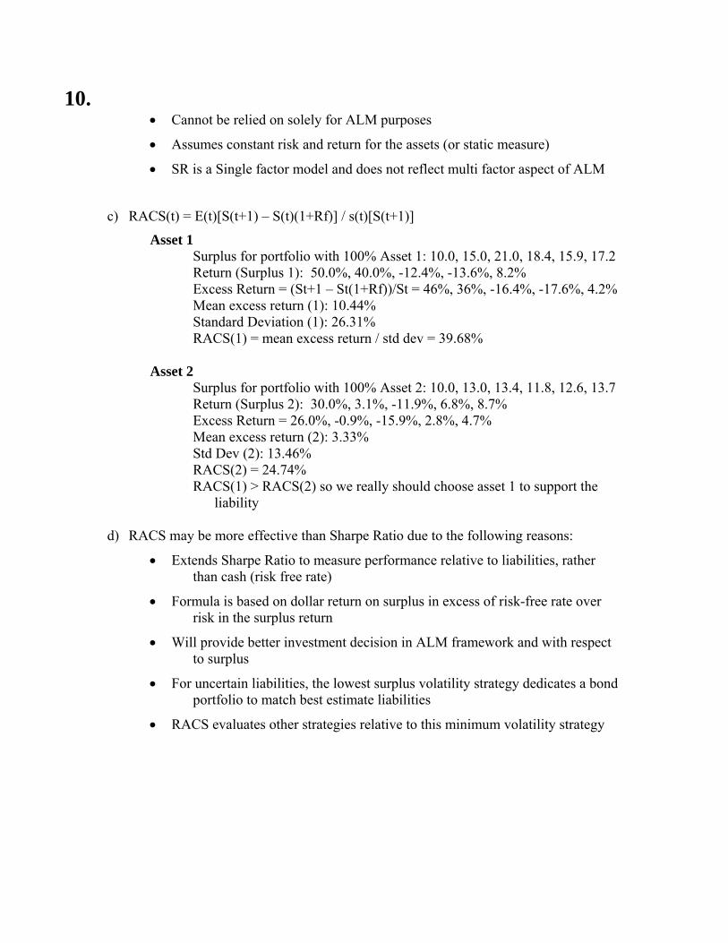
10. • Cannot be relied on solely for ALM purposes

• Assumes constant risk and return for the assets (or static measure)

• SR is a Single factor model and does not reflect multi factor aspect of ALM

c) RACS(t) = E(t)[S(t+1) – S(t)(1+Rf)] / s(t)[S(t+1)]

Asset 1 Surplus for portfolio with 100% Asset 1: 10.0, 15.0, 21.0, 18.4, 15.9, 17.2 Return (Surplus 1): 50.0%, 40.0%, -12.4%, -13.6%, 8.2% Excess Return = (St+1 – St(1+Rf))/St = 46%, 36%, -16.4%, -17.6%, 4.2% Mean excess return (1): 10.44% Standard Deviation (1): 26.31% RACS(1) = mean excess return / std dev = 39.68%

Asset 2

Surplus for portfolio with 100% Asset 2: 10.0, 13.0, 13.4, 11.8, 12.6, 13.7 Return (Surplus 2): 30.0%, 3.1%, -11.9%, 6.8%, 8.7% Excess Return = 26.0%, -0.9%, -15.9%, 2.8%, 4.7% Mean excess return (2): 3.33% Std Dev (2): 13.46% RACS(2) = 24.74% RACS(1) > RACS(2) so we really should choose asset 1 to support the

liability d) RACS may be more effective than Sharpe Ratio due to the following reasons:

• Extends Sharpe Ratio to measure performance relative to liabilities, rather than cash (risk free rate)

• Formula is based on dollar return on surplus in excess of risk-free rate over risk in the surplus return

• Will provide better investment decision in ALM framework and with respect to surplus

• For uncertain liabilities, the lowest surplus volatility strategy dedicates a bond portfolio to match best estimate liabilities

• RACS evaluates other strategies relative to this minimum volatility strategy

11. Learning Outcomes: 2d) Establish appropriate benchmarks for a portfolio and understand how to measure

performance against those benchmarks. 6c) Describe best practices in credit risk measurement, modeling and management. 6f) Describe risk mitigation techniques and practices: credit derivatives,

diversification, concentration limits, and credit support agreements. This question tests students’ knowledge of various credit-related securities, and of their appropriateness in a dedicated portfolio for a terminated defined benefit pension plan. Solution: a) A dedicated portfolio is a cash-flow matching portfolio. It is usually expensive to

match cash flows. Process:

• Define the characteristics of the liabilities, and estimate future liability cash flows.

• Since this is a terminated plan, may be easier as there will be no new entrants. (Closed block)

• Uncertainties will arise due to mortality and other factors. Review mortality, termination, and benefit assumptions. Validate actual versus projected experience.

• Set portfolio constraints. Determine which assets are allowed and aren’t. (Sector, quality, issuer, lot sizes). Probably don’t want callable bonds (cash flow uncertainty) or below investment grade debt (possible default).

• Set model reinvestment rate. Cash flows will probably not match exactly, so there is a need for an assumed rate for reinvestment. The more conservative your assumption, the tighter the optional cash flow math. Balance aggressive yields against risk of default, as you want to cover liability cash flows with high probability.

• Select optimal portfolio (lowest cost). You’ve already set your constraints,

and you’re just trying to match cash flows. • As interest rates change, you’ll want to re-optimize your portfolio as possible

to reduce costs, or bond swaps for better yield or credit ratings. Be careful to preserve cash flow match.

11. b) 1. Credit default swap

A CDS is a credit derivative where buyer pays a periodic premium (until a credit event occurs) for “credit insurance”. If a contractually defined credit even occurs for the specified company, buyer of protection holds right to sell bonds issues by the company for face value. Seller of the insurance agrees to buy the bonds for face value when a credit event occurs. Settlement could be physical or cash. A CDS can be used to convert a corporate bond into a risk free bond. Risk of prepayment does not make the CDS a suitable security for a dedicated portfolio strategy.

2. Collateralized debt obligations

A CDO produces securities with different risk characteristics, including some high quality debt, from a portfolio of debt instruments including average quality debt. CDO issuer issues different tranches (senior mezzanine, equity) with different credit exposure, each with a different proportion of the bond principal and risk of default. Each tranche earns a different yield depending on the risk and the yield is only paid on the remaining principal after losses have been paid. The equity tranche is riskiest and absorbs all initial losses up to the proportion invested. The next tranche absorbs the credit losses beyond equity up to its proportion invested. Senior tranche is usually investment grade. A high tranche can be a good choice for a dedicated portfolio since it has a low default risk and high credit rating. Lower tranches are not good investments for a dedicated strategy due to the higher default risk.

3. Convertible bonds

Convertible bond has option to convert bond to pre-specified number of shares of issuer’s stocks in the future. These bonds are usually callable, but the holder can convert once the bond is called. (forced conversion) Credit risk should be considered when valuing convertible bonds as payments are subject to credit risk. Not a good choice for a dedicated portfolio due to call feature.

12. Learning Outcomes: 3d) Apply different types of asset allocation strategies and evaluate traditional

alternative asset classes. This recall question tests students’ knowledge of basic hedge fund characteristics. See Litterman chapter 26. Solution:

a) Contrast the investment constraints faced by hedge fund managers versus conventional

investment managers 1) Hedge fund mangers do not face the same constraint on short positions that traditional

active mangers face 2) Hedge fund mangers are not limited to securities that are only part of a selected

performance benchmark which is typically a constraint for active mangers. 3) Hedge fund mangers are not restricted to an investment style for which they were selected.

Hedge fund mangers can quickly change portfolio characteristics to reflect changes in market conditions. Traditional active mangers, by contrast, are usually restricted to the investment style for which they were selected.

4) Hedge funds allow the use of leverage 5) Limited regulatory oversight for hedge funds b) Describe two ways to implement a hedge fund allocation. 1) "Portable Alpha" strategy - Investors can treat the hedge fund portfolio as a substitute for other active strategies 2) Outright allocation to hedge funds in the same way that allocations are made to other asset

classes - Investor can substitute away from equity holdings into the hedge fund portfolio - Investor can substitute away from bonds into the hedge fund portfolio c) Explain how hurdle rates can be used to justify a reallocation of assets to hedge funds. 1) Implied hurdle rates are the minimum returns required to invest at a particular level in a

hedge fund portfolio with specific risk characteristics 2) Total portfolio volatility declines almost linearly with allocations to hedge fund 3) The principal reason for this is that we are effectively substituting an asset with low

volatility for one with higher volatility (infrequent pricing lead to lower vols)

13. Learning Objectives: 1e) Explain how numerical methods can be used to effectively model complex assets

or liabilities. This question tests candidates’ knowledge of explicit finite different method and Crank-Nicolson method in valuing a derivative. Solution: An investment co-worker created the following table of put option values using the finite difference method. However, one cell in the grid was left blank. The details of the put option are:

• Strike Price = 10 • Annual volatility = 30% • Risk free rate = 5% • Annual dividend rate = 2%

Time to Maturity (in months)

Stock Price 3 2 1 0 20 0.0000 0.0000 0.0000 0.0000 15 0.0094 0.0049 0.0017 0.0000 10 0.1734 0.1178 0.0601 0.0000 5 4.9040 4.9673 5.0000 0 10.0000 10.0000 10.0000 10.0000

a) Calculate the value of the missing cell using the explicit finite difference method.

, 1, 1 1, 1, 1i j j i j j i j j i jf a f b f c f∗ ∗ ∗+ − + + += + +

( ) 2 21 1 11 2 2ja r q j t j t

r rσ∗ ⎛ ⎞= − − Δ + Δ⎜ ⎟+ Δ ⎝ ⎠

( )2 21 11jb j t

r tσ∗ = − Δ

+ Δ

( ) 2 21 1 11 2 2jc r q j t j t

r tσ∗ ⎛ ⎞= − Δ + Δ⎜ ⎟+ Δ ⎝ ⎠

( ) 2 21

1 1 1 1 10.05 0.02 1 0.3 11 2 12 2 121 0.05

12

a∗ ⎡ ⎤⎛ ⎞ ⎛ ⎞ ⎛ ⎞= − − × × × × × ×⎜ ⎟ ⎜ ⎟ ⎜ ⎟⎢ ⎥⎛ ⎞ ⎝ ⎠ ⎝ ⎠ ⎝ ⎠⎣ ⎦+ ×⎜ ⎟⎝ ⎠

= 0.00249

13. 2 2

11 11 0.3 1 0.98838

1 121 0.0512

b∗ ⎡ ⎤⎛ ⎞= − × × =⎜ ⎟⎢ ⎥⎛ ⎞ ⎝ ⎠⎣ ⎦+ ×⎜ ⎟⎝ ⎠

( ) 2 21

1 1 1 1 10.05 0.02 1 0.3 11 2 12 2 121 0.05

12

c∗ ⎡ ⎤⎛ ⎞ ⎛ ⎞ ⎛ ⎞= − × × + × × ×⎜ ⎟ ⎜ ⎟ ⎜ ⎟⎢ ⎥⎛ ⎞ ⎝ ⎠ ⎝ ⎠ ⎝ ⎠⎣ ⎦+ × ⎜ ⎟⎝ ⎠

= 0.00498

1,1 0.00249 10 0.98839 4.9673 0.00498 0.0601 4.9348f = × + × + × = b) Describe the Crank-Nicolson method and compare it to the explicit finite difference method.

The Crank-Nicolson method uses both implicit and explicit differentiation and averages them. It converges faster but is still time consuming.

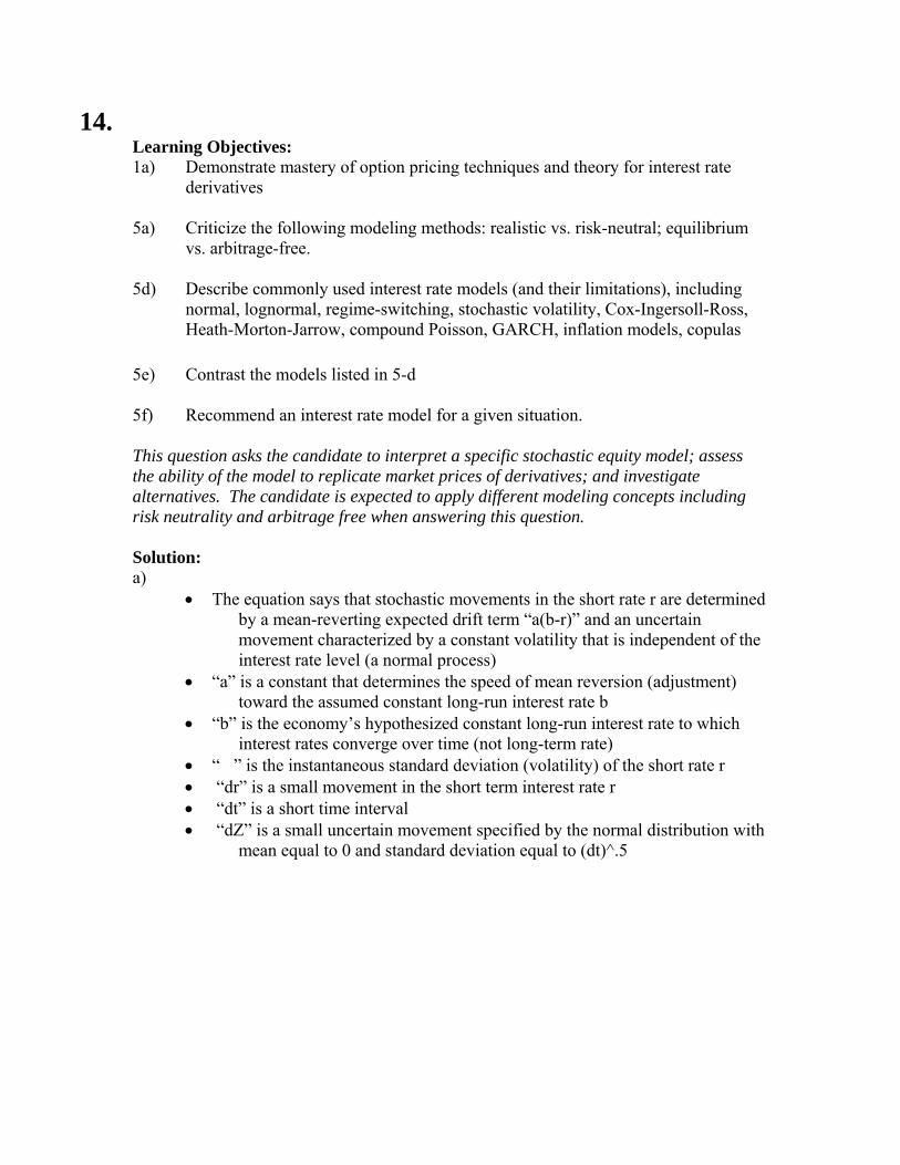
14. Learning Objectives: 1a) Demonstrate mastery of option pricing techniques and theory for interest rate

derivatives 5a) Criticize the following modeling methods: realistic vs. risk-neutral; equilibrium

vs. arbitrage-free. 5d) Describe commonly used interest rate models (and their limitations), including

normal, lognormal, regime-switching, stochastic volatility, Cox-Ingersoll-Ross, Heath-Morton-Jarrow, compound Poisson, GARCH, inflation models, copulas

5e) Contrast the models listed in 5-d 5f) Recommend an interest rate model for a given situation. This question asks the candidate to interpret a specific stochastic equity model; assess the ability of the model to replicate market prices of derivatives; and investigate alternatives. The candidate is expected to apply different modeling concepts including risk neutrality and arbitrage free when answering this question. Solution: a)

• The equation says that stochastic movements in the short rate r are determined by a mean-reverting expected drift term “a(b-r)” and an uncertain movement characterized by a constant volatility that is independent of the interest rate level (a normal process)

• “a” is a constant that determines the speed of mean reversion (adjustment) toward the assumed constant long-run interest rate b

• “b” is the economy’s hypothesized constant long-run interest rate to which interest rates converge over time (not long-term rate)

• “�” is the instantaneous standard deviation (volatility) of the short rate r • “dr” is a small movement in the short term interest rate r • “dt” is a short time interval • “dZ” is a small uncertain movement specified by the normal distribution with

mean equal to 0 and standard deviation equal to (dt)^.5

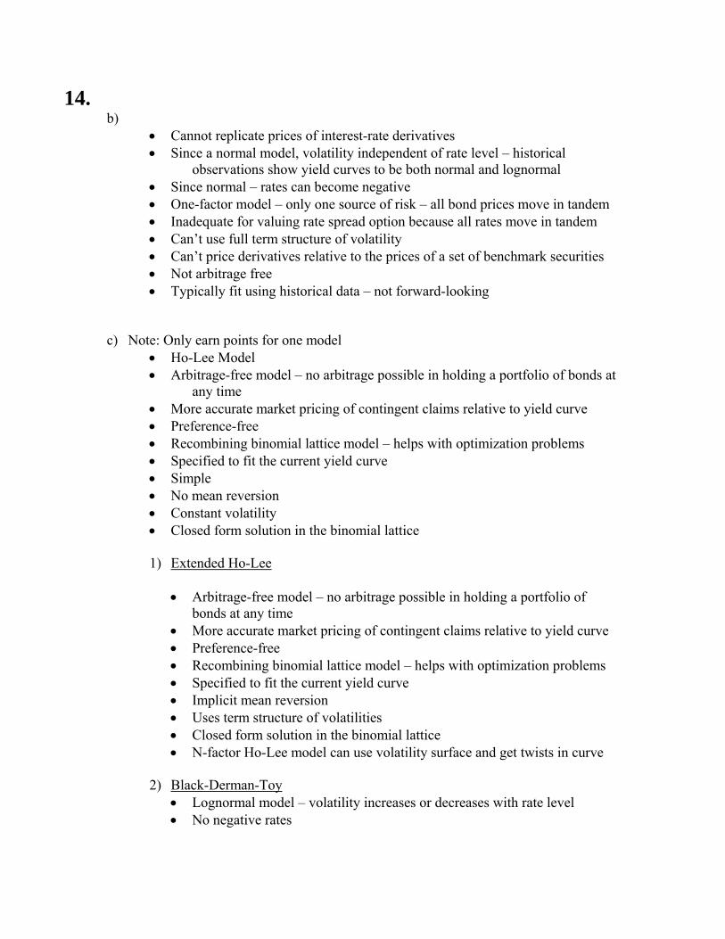
14. b)

• Cannot replicate prices of interest-rate derivatives • Since a normal model, volatility independent of rate level – historical

observations show yield curves to be both normal and lognormal • Since normal – rates can become negative • One-factor model – only one source of risk – all bond prices move in tandem • Inadequate for valuing rate spread option because all rates move in tandem • Can’t use full term structure of volatility • Can’t price derivatives relative to the prices of a set of benchmark securities • Not arbitrage free • Typically fit using historical data – not forward-looking

c) Note: Only earn points for one model

• Ho-Lee Model • Arbitrage-free model – no arbitrage possible in holding a portfolio of bonds at

any time • More accurate market pricing of contingent claims relative to yield curve • Preference-free • Recombining binomial lattice model – helps with optimization problems • Specified to fit the current yield curve • Simple • No mean reversion • Constant volatility • Closed form solution in the binomial lattice

1) Extended Ho-Lee

• Arbitrage-free model – no arbitrage possible in holding a portfolio of

bonds at any time • More accurate market pricing of contingent claims relative to yield curve • Preference-free • Recombining binomial lattice model – helps with optimization problems • Specified to fit the current yield curve • Implicit mean reversion • Uses term structure of volatilities • Closed form solution in the binomial lattice • N-factor Ho-Lee model can use volatility surface and get twists in curve

2) Black-Derman-Toy

• Lognormal model – volatility increases or decreases with rate level • No negative rates

14. • Arbitrage-free model – no arbitrage possible in holding a portfolio of

bonds at any time • More accurate market pricing of contingent claims relative to yield curve • Preference-free • Recombining binomial lattice model – helps with optimization problems • Specified to fit the current yield curve • Implicit mean reversion • Uses term structure of volatilities

3) Hull-White

• Arbitrage-free model – no arbitrage possible in holding a portfolio of bonds at any time

• More accurate market pricing of contingent claims relative to yield curve • Explicit mean reversion term • Preference-free • Recombining trinomial lattice model – helps with optimization problems • Specified to fit the current yield curve • Forward volatility is constant • Closed form solution in continuous time formulation • Other relevant points from readings

4) H-J-M

• Arbitrage free • Model of forward rates • Uses volatility surface to specify an arbitrage-free rate model • Flexible • Drift and volatility terms determined by bond volatilities • Non-recombining tree - so usually use Monte Carlo simulation

d)

• No. An arbitrage free model uses risk-neutral probabilities, not market probabilities

• An economic (equilibrium) model can reflect the supply and demand for funds in the economy, fiscal policy, other macroeconomic policies

• An economic (equilibrium) model can be used to extrapolate values • It can relate the yield curve to economic factors • It can be fitted using historical yield data

15. Learning Objectives: 3f) Embedded Options: Complete analysis that may include calculation of hedging

cost, deterministic and stochastic analysis of cash flow, reserves, and capital levels under a range of economic environments.

1a) Demonstrate mastery of option pricing techniques and theory for equity (including exotic options) and interest rate derivatives.

This question asks the candidate to apply the textbook option pricing tools to hedge a GMAB. Data templates and intermediate values hint at the solution, which is based on Hardy chapter 8 and Hull chapters 13-14.

Solution: a) Put price formula for stock with no dividends:

( ) ( )( ) ( )

2 1

2

1 2 1

ln / 2,

rTp Ke N d S N d

S K r Twhere d d d T

T

σσ

σ

−= − − −

+ += = −

When the stock pays dividends at the annual effective rate m, the S in the above formula will be replaced by S(1-m)T Therefore the put prices given in the table can be considered as the values ( ) ( )( )1 , ,T

Sp P T BSP S m G T= = −

i.e. the table gives the following values: ( ) ( )( )1 ,1,tP t BSP m t= −

( ) ( )( )1

1 0 11 , ,tSP t BSP S m G t= −

( ) ( )1 1 1SP t P t=

( ) ( ) ( )( ) ( )1

2 2 0 1 2 11 tSP t S m P t P t t= − + −

( ) ( ) ( )( ) ( ){ } ( )2 2 1

3 3 0 1 2 2 3 21 1t t tSP t S m P t m P t P t t−= − + − + −

GMAB survival benefit hedge cost: ( ) ( ) ( ) ( ) ( ) ( ) ( )

1 2 31 1 2 2 3 30 t x t x t xH P t p P t p P t pτ τ τ= + + Substituting t1 = 3, t2 = 13, t3 = 23, S0 = 1, G = 1.2, m = 0.03

15. ( ) ( )( )3

1 1 0.03 ,1.2,3SP t BSP= −

This is the value in the table with S0/K = 1/1.2 and T=3 P1(3) = 0.2335 P(t2 – t1) = P(t3 – t2) = P(10) = BSP(.710,1,10) => P(10)=0.14703 This is the value in the table with S0/K = 1 and T=10 P(10) = 0.14703 P2(13) = ((1 – m)3 + PS(3)) P(13 – 3) P2(13) = (0.973 + 0.2335) * 0.14703 = 0.1685 b)

The hedge cost will be separated for bond and stock parts Option delta is the number of stock shares to be shorted Discrete time hedging will lead to hedging errors Hedging error may be modeled through time-based or move-based strategy Consider transaction costs, which are not included in B-S-M.

16. Learning Objectives: 5d) Describe commonly used equity models (and their limitations) 5e) Contrast equity models 5f) Recommend an equity model for a given situation This is an application question asking candidates to demonstrate mastery of the lognormal and regime-switching models for generating equity returns. The candidates were also expected to show understanding of limitations of the models (especially as they relate to capturing extreme price movements and volatility clustering), as well as the advantages and disadvantages of using these models for a given situation. The best sources for answering this question could be found in chapters 1, and 2 of the Hardy “Investment Guarantees: Modeling and Risk Management for Equity-Linked Life Insurance” textbook. Credit was also given for answers based on other readings from the syllabus resources if relevant.

Solution: a. Under LN

( )2 0P S S<

2

0ln 0SP

S⎛ ⎞⎛ ⎞

= <⎜ ⎟⎜ ⎟⎜ ⎟⎝ ⎠⎝ ⎠

0 22

N μσ

−⎛ ⎞= ⎜ ⎟⎝ ⎠

( )0.2382N= − = 0.406

Under RSLN2 First calculate P (# of months spent in regime 1=K)

0.1896 0.82650.1896 0.0398

π = =+

( ) ( ) ( ) ( ) ( )2 210 0 1 1 1 0.8265 1 0.1896P Pπ π= × + − × − = − × − = 0.1406

( ) ( ) ( )2 12 211 1 0.8265 .0398 1 .8265 .1896P P Pπ π= × + − = × + − × = .0658

( ) ( ) ( )2 2 22 1 0 1 0.7936P P P= − − =

16. k kμ kσ 0 22 0.0322μ = − 2

22 0.1058σ = 1 1 2 0.0034μ μ+ = − 2 2

1 2 0.0825σ σ+ = 2 12 0.0254μ = 2

12 0.0492σ =

0k = ( )2 0P S S<

0.03220.1058

N −⎛ ⎞= −⎜ ⎟⎝ ⎠

( )0.3048N= 0.6195=

1k = ( )2 0P S S<

0.00340.0825

N −⎛ ⎞= −⎜ ⎟⎝ ⎠

( )0.0412N= 0.5165=

2k = ( )2 0P S S<

0.02540.0492

N ⎛ ⎞= −⎜ ⎟⎝ ⎠

( )0.5163N= − .3028= Prob 0.6195 0.1406 0.5165 0.0658 0.0328 0.7936= × + × + × .3028= b)

• Density function of LN is easily calculated • RSLN is more complex • RSLN assumes a discrete process switching between LN • Both density functions have an asymmetric bell shape with elongated right

side • RSLN has fatter tail • LN has taller peak

c)

• Lognormal model is a traditional approach • LN provides adequate approximations over short time intervals

16. • Not over long term intervals • Does not capture extreme price movements, autocorrelation or volatility

clustering • Have to thin a tail

RSLN Model

• Market process switches between regimes • Market does switch between stable one (bull) and unstable one (bear) • Easy way to create stochastic volatility • Provides a much larger left tail so better for maturity guarantee • Does provide volatility clustering • RSLN matches historical return well • RSL is a more complex model but still tractable

17. Learning Objectives: 5g) Describe issues in the estimation or calibration of financial models. This question asks the candidates to demonstrate knowledge of an application of EMWA and GARCH(1,1) models, and describe the limitations of using maximum likelihood method to estimate the parameters to be used in the models.

Solution: a) .0626α = .8976β = .0398γ = GARCH (1,1)

LV = long term variance

2 2 21 1 1L n nV uσ γ α βσ− −= × + +

( ) ( )2 2tn t L n LE V Vσ α β σ+⎡ ⎤ = + + −⎣ ⎦

10t = 2 20.005nσ = 2.008LV =

• Given volatilities, need to convert to variance for calculations, then back to

volatilities for final answer

( ) ( ) ( ) ( )( )2 10 2 2210 .008 .0626 .8976 .005 .008nE σ +⎡ ⎤ = + + −⎣ ⎦

= .000038017 [ ]10 0.6166%nE σ + =

b) EWMA

2 2n i n i

iσ α μ −=∑ 1i iα λα+ =

• Weight given to observation i days ago ( )iα decreases exponentially at a rate

of ( )0 1λ λ≤ ≤ , the rate of decay • More weight given to recent observations

• Makes updating estimate easy

( )2 2 2

1 11n n nσ λ σ λ μ− −= × + − 2

1nμ − =Estimate of true daily volatility

17. • No weight given to a long-run volatility • Not mean reverting

GARCH (1,1) 2 2 2

1 1n l n nVσ γ αμ βσ− −= × + +

• Gives weight to a long-run average volatility ( )2V

• Easy to update estimates as well • Weight given to observation i days ago decreases exponentially at a rate of β

• EWMA is a special case when 0γ = , β λ= , 1α λ= − • GARCH(1,1) is a mean-reverting model • Theoretically appealing as volatilies do tend to mean revert • Can be used to project expected future vols (see part 1a.)

( ) ( )2 2tn E L n LE V Vσ α β σ+⎡ ⎤ = + + −⎣ ⎦

As t →∞ , expected value LV→ (mean reverting) c)

1. MLE estimates do not apply (are not appropriate) for models that are not strictly stationary

2. Large sample sizes usually needed to produce reliable results 3. If parameters estimated near the boundary, they cannot be trusted 4. MLE parameter may be a good bit for the model, but the model with the

parameter may not be a good fit for the date Additional

Condition required for parameter constraints EMWA 1 1 1α β+ = GARCH 2 2 1γ α β+ + =

18. Learning Outcomes: 2b) Distinguish relative VaR, marginal VaR, increment VaR and CTE. This question tests students’ knowledge of different VaR measurements, as well as testing their ability to apply these in assessing a hedge strategy. Solution: a)

1. VaR i i iWασ=

VaR ( )( )$1.645 .06 10 $987,000A M= =

VaR ( )( )$1.645 .02 10 $329,000B M= =

2. Portfolio VaR = $1.645 448,000 1.1pW Mασ = =

Where ( )$

2 $ $$

.0036 .00024 1010 10

.00024 .0004 10p

MW M M

Mσ

⎡ ⎤−⎛ ⎞⎡ ⎤= − ⎢ ⎥⎜ ⎟⎣ ⎦ − −⎝ ⎠ ⎢ ⎥⎣ ⎦

( )( )

$ $

,,

.038410 10

.0064

A PB P

CoV R RCoV R R

M M

⎡ ⎤=⎢ ⎥⎣ ⎦

⎡ ⎤⎡ ⎤− ⎢ ⎥⎣ ⎦ −⎣ ⎦14243

= 448,000 Where -.00024 = p ( )( )( ).2 .06 .02A Bσ σ = − Undiversified VaR = sum of individual VaR (from parti) = 987,000 + 329,000 = 1,316,000 Diversification effect = Undiversified VaR = portfolio VaR

= 216,000 3. Marginal VaR is an approximation for how much the portfolio VaR will

change for a $1 increase to position i ( ),i p

ip

Cov R RVaR α

σΔ = × ( ),i pCov R R - calculated in part 2.

.0384

.0064⎡ ⎤

= ⎢ ⎥−⎣ ⎦

.0384 11.645

.0064 448,000⎡ ⎤

= × ×⎢ ⎥−⎣ ⎦

18. .0944.0157

⎡ ⎤= ⎢ ⎥−⎣ ⎦

.0944AVaR∴Δ =

.0157BVaR∴Δ = − In summary, an increase in long position of Asset A of $1 will increase

portfolio VaR by 9.5 centers. Likewise, a $1 increase in long position of asset B (or decrease of $1 in short position) will decrease portfolio VaR by 1.6 cents.

4. Component VaR = marginal i iVaR W×

Component VaR ( )$.0944 10 940,000A M= =

Component VaR ( )$.0157 10 157,000B M= − − =

These values indicate that if asset A is sold, the portfolio VaR would decrease by $940,000. If short position of B is liquidated, te portfolio VaR would decrease by 157,000.

b) Short position of asset B is not an effective hedge. Since the diversification benefit of

B is negative, adding short-position B increases the portfolio VaR. It would actually be more effective to hold a long position in B.

c) Financial institution should take a long position in B.

Best hedge a* ( )2

,W Cov B portfolioiσ

− ×=

( ) ( ) ( )( )( )

( )

2

2

10 .02 10 .2 .06 .02

.02

M M⎡ ⎤− × + −⎣ ⎦=

=$16M ∴, Minimize risk by taking a $16M long position in asset B. Net position will be ( ) ( )$ $ $10 16 6M M long M− + =

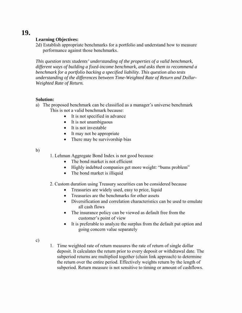
19. Learning Objectives: 2d) Establish appropriate benchmarks for a portfolio and understand how to measure

performance against those benchmarks. This question tests students’ understanding of the properties of a valid benchmark, different ways of building a fixed-income benchmark, and asks them to recommend a benchmark for a portfolio backing a specified liability. This question also tests understanding of the differences between Time-Weighted Rate of Return and Dollar-Weighted Rate of Return. Solution: a) The proposed benchmark can be classified as a manager’s universe benchmark

This is not a valid benchmark because: • It is not specified in advance • It is not unambiguous • It is not investable • It may not be appropriate • There may be survivorship bias

b)

1. Lehman Aggregate Bond Index is not good because • The bond market is not efficient • Highly indebted companies get more weight: “bums problem” • The bond market is illiquid

2. Custom duration using Treasury securities can be considered because

• Treasuries are widely used, easy to price, liquid • Treasuries are the benchmarks for other assets • Diversification and correlation characteristics can be used to emulate

all cash flows • The insurance policy can be viewed as default free from the

customer’s point of view • It is preferable to analyze the surplus from the default put option and

going concern value separately c)

1. Time weighted rate of return measures the rate of return of single dollar deposit. It calculates the return prior to every deposit or withdrawal date. The subperiod returns are multiplied together (chain link approach) to determine the return over the entire period. Effectively weights return by the length of subperiod. Return measure is not sensitive to timing or amount of cashflows.

19. 2. Dollar weighted rate of return is an internal rate of return calculation on the

portfolio. It is the average returned earned on all money invested. It is sensitive to the timing and size of cashflows.

d)

1. Appropriate benchmark for an investment manager would be a custom security benchmark. The manager should be measured using a time weighted rate of return since managers do not have control over timing or size of cashflows.

2. The profitability of a block of business should be measured on a dollar

weighted rate of return basis. The benchmark should consider the liability cashflows since it is part of the profitability.

20. Learning Objectives: 4a) Identify and apply the concepts of behavioral finance with respect to option holder

behavior, including the assessment of optimal behavior, real behavior, model behavior, and empirical studies.

4b) Explain how behavioral characteristics of individuals or firms affect the investment

or capital management process. 4d) Explain why a historical equity risk premium may not be indicative of future

expectations This question tests students’ knowledge of future equity return expectations, and also knowledge of theories that can explain some market anomalies. Solution: a) Historical equity returns have been high. New justified price/earning ratios are likely higher in the new economy due to

• more stable economy, reduction in volatility • technical advancement • operational efficiency • lower transaction cost on equity • favorable tax structure for equity

Future returns could be lower than historical due to

• future uncertainty such as terrorism • age wave – baby boomer taking income from equity investment

b) Twin shares: two types of shares with fixed relative claims on cash flows and assets of the firm.

Example: Royal Dutch and Shell. Anomaly is created when the share prices no longer maintain fixed relationship. Law of One Price is broken. Arbitrage can be created by buying cheaper version and selling expensive one. However, arbitrage may not work over a fixed time period.

When Shell was included in the popular S&P 500 index, fund managers bought Shell, thus drove the relative price of Shell above Royal Dutch.

c) According to Market Efficient Hypothesis, market returns follow s a random walk pattern. However, studies have shown negative serial correlation over long holding periods indicating long-term reversion to mean. One explanation is market overreaction to information. There is herd mentality that investors buy rising stocks, which further increase the prices. Investors also tend to be overconfident. This explains Contrarian investment strategy.

21. Learning Objectives: 6c) Describe best practices in credit risk measurement, modeling and management 6e) Define credit risk as related to derivatives. Define credit risk as related to reinsurance

ceded counter party risk . Describe the use of comprehensive due diligence and aggregate counter-party exposure limits

6f) Describe risk mitigation techniques and practices: credit derivatives, diversification,

concentration limits, and credit support agreements This question tests students’ knowledge of credit risk mitigation, and specifically, end-users and applications of credit risk derivatives. Solution:

Banks could use the following to traditionally manage credit risk a) Termination/Reassignment clauses – Takes over in the event of a downgrade or default b) Letters of credit/corporate guarantees/portfolio insurance c) Embedded put options When credit quality deteriorates d) Collateralizations – Pledge assets to soften impact of credit event Can be at outset or at agreed event e) Netting If one of the counterparties issues default, even if in a positive position f) Marking to Market Daily each counterparty posts margin in an account Eliminates credit risk because only one days change to market value if

default

Users of Credit a) Banks Credit rate shifter b) Investors/Financial Institutions Yield Enhancers

Credit Derivatives

a) Credit Linked Notes – b) Total Return Swaps c) Credit Intermediation swap – third party manages the deal to lessen credit risk

21. d) Credit Default swap Protection buyer and seller Event and amount of coverage well defined in advance Materiality clause e) Credit Spread Options – Pays (max (spread – strike,0) * notional * modified duration f) CDO’s g) Synthetic CDO’s

Securitization

CDOs are a way for a counterparty to securitize a bond portfolio and reslice them into different credit quality bonds. There are three tranches. The senior tranche is highest quality, mezzanine tranch of good quality and a risky equity tranche. Returns vary based on seniority. CDO holder retains equity tranche. It has lower regulatory capital and is less costly to hold.

22. Learning Objectives: 3c) Develop a portfolio appropriately supporting liabilities. Set portfolio policy and

objectives, specifying asset selection criteria, incorporate capital market expectations and risk management strategies including hedging.

This question tests understanding of the risk/return tradeoff when constructing a portfolio to support a liability, in this case a traditional defined benefit pension plan. See study notes 8V-323-05 and 8V-113-00.

Solution: (a) Explain the Company's financial risk exposure from the pension plan.

• Low asset returns can reduce surplus (increase the deficit) • Low interest rates increase the liabilities of pension plans and can reduce

surplus (increase the deficit). • Deficits impair the Company's balance sheet, increase the future cash

contribution and lower net income. • Not capable of paying benefits promised

Regulators may interfere Other explicit risks are: Longevity risk, Interest risk, Market or investment risk (b) Compare and contrast the following efficient frontier methodologies: i) Traditional ii) Lower Partial Moment iii) Surplus

i) Traditional efficient frontier :

• Based on asset only study • Investor has quadratic utility fonction • Mean-Variance approach / efficient frontier • Symetric consideration of return (up movement is risky)"

ii) Lower Partial Moment :

• Uses only the left-hand tail of the return distribution. • Also an asset-only approach. • Captures an investor's preferences for downside risk tolerance

22. • Mean LP second moment portfolios are more efficient than the

traditional mean-variance efficient frontier • Some computational difficulties

• Requires a treshold or benchmark to be decided • Good for distribution that is not normal • More intuitive and representative of the investors’ concerns

iii) Surplus efficient frontier methodology :

• Uses the net of assets and liabilities • Looks at surplus return vs surplus risk (or variance) • The surplus efficient frontier is a benchmark to measure the

plan sponsor's risk aversion and risk tolerance Liab is like a negative asset with positive volatility

• Basis for ALM (c) Recommend an efficient frontier methodology for the Company's pension plan.

• Recommend the surplus efficient frontier methodology • Goal is to choose an asset allocation that will shrink the deficit (increase the

surplus) • Controlling the volatility of the surplus • Reflect Funding Ratio / must consider Liabilities for pension plan • Goal of DB plan is not profit, but to fund future benefits • Appropriate benchmarking

23. Learning Objectives: 5c) Define and apply the concepts of martingale, market price of risk and measures in

single and multiple state variable contexts. This question verifies the knowledge of different concepts associated with martingales.

The candidate is also asked to apply these concepts in the case of a simple change in numeraire.

Solution:

(a)(i) A martingale is a zero-drift, stochastic process, can be expressed as dθ = σ dz, where z is a Wiener process.

The variable θ could depend on θ itself and other stochastic variables. Its expected value at any future time = its value today. i.e., E(θT) = θ0

(a)(ii) numeraire refers to the security price that is used as the unit to measure another security

price typically with the same source of uncertainty. (a)(iii) Define Ф = f / g where f, g are stochastic processes depending on the same source of

uncertainty. The equivalent martingale measure says that, when there is no arbitrage opportunity.

Ф is a martingale for some choice of market price of risk. Further, if the choice of market price of risk is the volatility of g, then the ratio of f / g is a martingale for all securities f.

(a)(iv) forward risk neutral refers to a world where the market price of risk is the volatility of the

numeraire, with respect to g. (b) In the forward risk-neutral world with respect to g, the market price of risk is set to the

volatility of g and the process f /g simplifies to a martingale process, so the expected growth rate = 0.

D (f / g) = (σf – σg )(f / g) dz, so the volatility of f / g is (σf - σg )(f / g)