1. introduction amld { deep learning in pytorch · ì éiè"ä ì ûkè ç ï ï uÄ ï è©ì...

AMLD – Deep Learning in PyTorch

1. Introduction

Francois Fleuret

http://fleuret.org/amld/

February 10, 2018

ÉCOLE POLYTECHNIQUEFÉDÉRALE DE LAUSANNE

Why learning

Francois Fleuret AMLD – Deep Learning in PyTorch / 1. Introduction 2 / 56

Many applications require the automatic extraction of “refined” informationfrom raw signal (e.g. image recognition, automatic speech processing, naturallanguage processing, robotic control, geometry reconstruction).

(ImageNet)


Our brain is so good at interpreting visual information that the “semantic gap”is hard to assess intuitively.

This is a horse


>>> from torchvision import datasets

>>> cifar = datasets.CIFAR10 (’./data/cifar10/’, train=True , download=True)

Files already downloaded and verified

>>> x = torch.from_numpy(cifar.train_data)[43]. transpose (2, 0).transpose (1, 2)

>>> x.size()

torch.Size([3, 32, 32])

>>> x.narrow(1, 0, 4).narrow(2, 0, 12)

(0 ,.,.) =

99 98 100 103 105 107 108 110 114 115 117 118

100 100 102 105 107 109 110 112 115 117 119 120

104 104 106 109 111 112 114 116 119 121 123 124

109 109 111 113 116 117 118 120 123 124 127 128

(1 ,.,.) =

166 165 167 169 171 172 173 175 176 178 179 181

166 164 167 169 169 171 172 174 176 177 179 180

169 167 170 171 171 173 174 176 178 179 182 183

170 169 172 173 175 176 177 178 179 181 183 184

(2 ,.,.) =

198 196 199 200 200 202 203 204 205 206 208 209

195 194 197 197 197 199 200 201 202 203 206 207

197 195 198 198 198 199 201 202 203 204 206 207

197 196 199 198 198 199 200 201 203 204 207 208

[torch.ByteTensor of size 3x4x12]


Extracting semantic automatically requires models of extreme complexity, whichcannot be designed by hand.

Techniques used in practice consist of

1. defining a parametric model, and

2. optimizing its parameters by “making it work” on training data.

This is similar to biological systems for which the model (e.g. brain structure) isDNA-encoded, and parameters (e.g. synaptic weights) are tuned throughexperiences.


A simple example is linear regression.

80

100

120

140

160

180

200

220

240

10 20 30 40 50 60 70 80

Sys

tolic

Blo

od P

ress

ure

(mm

Hg)

Age (years)

ModelData

Deep learning encompasses software technologies to scale-up to billions ofmodel parameters and as many training examples.


From artificial neural networks to “Deep Learning”


130 LOGICAL CALCULUS FOR NERVOUS ACTIVITY

b

e ~ ~

9

h

F I G ~ E 1

d

f

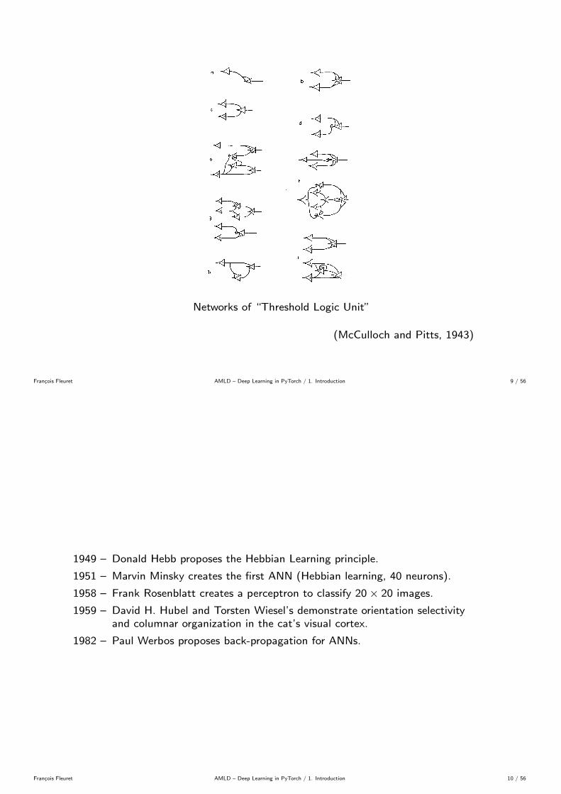
Networks of “Threshold Logic Unit”

(McCulloch and Pitts, 1943)


1949 – Donald Hebb proposes the Hebbian Learning principle.

1951 – Marvin Minsky creates the first ANN (Hebbian learning, 40 neurons).

1958 – Frank Rosenblatt creates a perceptron to classify 20× 20 images.

1959 – David H. Hubel and Torsten Wiesel’s demonstrate orientation selectivityand columnar organization in the cat’s visual cortex.

1982 – Paul Werbos proposes back-propagation for ANNs.


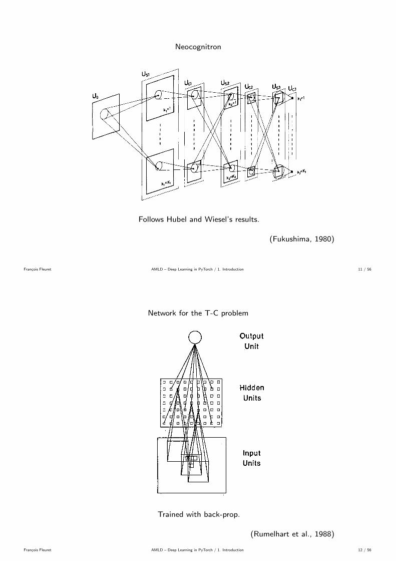
Neocognitron

195

visuo[ oreo 9l< QSsOCiQtion o r e o - -

lower-order --,. higher-order .-,. ~ .grandmother retino - - , - L G B --,. simple ~ complex --,. hypercomplex hypercomplex " - - cell '~

F- 3 I-- . . . . l r I I I I 11

Uo ', ~' Usl -----> Ucl t~-~i Us2~ Uc2 ~ Us3----* Uc3 T [ I L ~ L J

Fig. 1. Correspondence between the hierarchy model by Hubel and Wiesel, and the neural network of the neocognitron

shifted in parallel from cell to cell. Hence, all the cells in a single cell-plane have receptive fields of the same function, but at different positions.

We will use notations Us~(k~,n ) to represent the output of an S-cell in the kr th S-plane in the l-th module, and Ucl(k~, n) to represent the output of a C-cell in the kr th C-plane in that module, where n is the two- dimensional co-ordinates representing the position of these cell's receptive fields in the input layer.

Figure 2 is a schematic diagram illustrating the interconnections between layers. Each tetragon drawn with heavy lines represents an S-plane or a C-plane, and each vertical tetragon drawn with thin lines, in which S-planes or C-planes are enclosed, represents an S-layer or a C-layer.

In Fig. 2, a cell of each layer receives afferent connections from the cells within the area enclosed by the elipse in its preceding layer. To be exact, as for the S-cells, the elipses in Fig. 2 does not show the connect- ing area but the connectable area to the S-cells. That is, all the interconnections coming from the elipses are not always formed, because the synaptic connections incoming to the S-cells have plasticity.

In Fig. 2, for the sake of simplicity of the figure, only one cell is shown in each cell-plane. In fact, all the cells in a cell-plane have input synapses of the same spatial distribution as shown in Fig. 3, and only the positions of the presynaptic cells are shifted in parallel from cell to cell.

R3 ~I

modifioble synapses

) unmodifiable synopses

Since the cells in the network are interconnected in a cascade as shown in Fig. 2, the deeper the layer is, the larger becomes the receptive field of each cell of that layer. The density of the cells in each cell-plane is so determined as to decrease in accordance with the increase of the size of the receptive fields. Hence, the total number of the cells in each cell-plane decreases with the depth of the cell-plane in the network. In the last module, the receptive field of each C-cell becomes so large as to cover the whole area of input layer U0, and each C-plane is so determined as to have only one C-cell.

The S-cells and C-cells are excitatory cells. That is, all the efferent synapses from these cells are excitatory. Although it is not shown in Fig. 2, we also have

Fig. 3. Illustration showing the input interconnections to the cells within a single cell-plane

Fig. 2. Schematic diagram illustrating the interconnections between layers in the neocognitron

Follows Hubel and Wiesel’s results.

(Fukushima, 1980)


Network for the T-C problem

Trained with back-prop.

(Rumelhart et al., 1988)


LeNet-5

�� "! �

INPUT 32x32

Convolutions SubsamplingConvolutions

C1: feature maps 6@28x28

Subsampling

S2: f. maps6@14x14

S4: f. maps 16@5x5

C5: layer120

C3: f. maps 16@10x10

F6: layer 84

Full connectionFull connection

Gaussian connections

OUTPUT 10

��:LH%k%�#k¨Vb31A1*%: 01+@Ar06.%31+�2/}!PZ+�h;+r06K��#To,��w24CUMU24_L.#01:L24C%,/_!hX+@.%31,/_�hX+r0G8f2436g�T#*%+@31+b}�243fD%:LH4: 065�31+@A@24H4C%: 01:L24C�k lv,/AO*�>#_�,/C%+Y:L5�,§}�+B,R01.#31+�F�,/>ZT�:�k +4k%,§51+r0�2/}�.%C%: 0658X*#2451+Y8f+@:LH4*U015b,/31+YA@24C%5 0131,/:LC%+@D�012�Q�+�:LD#+BCU06:LA�,/_�k

å�ê©è"ç�ï1ëíï�å�è"ÿ�ä ï¾î�å�æ�ê�ø�éÆè ç�ï1æ�ä"ï�úiø�ì�ÿ�ê û�å%�aï�ädð&ã�ç�ï�è"ä�å�ø�é�å��û�ï��ì�ï,*¹��ø�ï�éiè�å�é�ù��ø�å�ê ��ì�éiè"ä ì�ûkè ç�ï�ïUÄ�ï��è©ì�ë¹è"ç�ï1ê"ø��î¼ì�ø�ùOé�ì�é!�û�ø�é�ïdå�ä ø³è@�að��}ëkè ç�ï��ì�ï,*¹��ø�ï�éiè ø�êpê�î�å�û�û1��è"ç�ï�é5è"ç�ï©ÿ�é�ø�è�ì�æNï�ä�åè ï�êø�é5å¹�iÿ�åaê�ø��}û�ø�é�ï�å�ä�î\ì�ù�ï��å�é�ù1è ç�ï©ê"ÿ�!�«ê"å�î\æ�û�ø�é��û�å%��ï�ä�î¼ï�ä ï�û��û�ÿ�ä�ê¼è"ç�ïOø�é�æ�ÿ�è�ð �}ë¸è ç�ï¤��ì�ï,*¹��ø�ï�éiè1ø�ê¾û�å�ä��aï��wê"ÿ�!�«ê å�î¼æ�û�ø�é��ÿ�é�ø�è ê{��å�é��ï�ê"ï�ï�é&å�êYæNï�ä"ëíì�ä î¼ø�é��¾å ��é�ìaø�ê��:ý�� ¼ìaä�åL��é�ìaø�ê��ñ{"� ¸ëíÿ�é��£è ø�ìaé¼ù�ï�æNï�é�ù�ø�é��®ì�éSè"ç�ïYúrå�û�ÿ�ï¹ì�ë�è ç�ï��ø�åaê�ðgþ�ÿ��ïdê@�ê"ø�úaïSû�å%��ï�ä êpì�ë��ì�é�úaì�û�ÿ�è"ø�ì�é�ê¸å�é�ù�ê"ÿ�!�«ê"å�î¼æ�û�ø�é��5å�ä ï�è@��æ�ø��å�û�û�å�û�è"ï�ä"é�åè"ïdùf��ä ï�ê"ÿ�û�è"ø�é��¾ø�éOå��øª�}æ��ä å�î\ø�ù B+wåèpï�å��ç&û�å%��ï�ä��è"ç�ïé�ÿ�î�Nï�ä¸ì�ëgëíïdåè ÿ�ä"ïSî�å�æ�ê�ø�êpø�é ��ä ï�å�ê"ï�ù&åaê è ç�ïSê"æ�å�è"ø�å�ûUä"ïdê�ìaû�ÿ!�è"ø�ì�é\ø�êUù�ï��ä ï�åaê�ïdù�ð (wå��ç©ÿ�é�ø³ègø�é�è ç�ï¹è"ç�ø�ä�ù�ç�ø�ù�ù�ï�éSû�å%��ï�äBø�é�©��?�ÿ�ä ï��¹î�å%��ç�årúaïgø�é�æ�ÿ�èb��ì�é�é�ï��£è ø�ìaé�ê�ëíä ì�î ê�ï�ú�ï�ä å�ûrëíï�åè ÿ�ä ï�î�å�æ�êø�é�è ç�ï æ�ä ï�ú�ø�ì�ÿ�ê�û�å%��ï�ä�ðkã�ç�ï��ìaé�ú�ì�û�ÿ�è ø�ìaé��ê"ÿ�!�«ê"å�î¼æ�û�ø�é��À��ì�îÀ��ø�é�åè ø�ìaé��ø�é�ê�æ�ø�ä ï�ù��&õ ÿ��ï�û�å�é�ù � ø�ïdê�ï�û< ê�é�ì�è"ø�ì�é�ê�ì�ë �"ê"ø�îÀ�æ�û�ï� ®å�é�ù �R��ìaî\æ�û�ï�£� ��ï�û�û�ê��ó¹åaêkø�î¼æ�û�ï�î¼ï�éaè ï�ù\ø�éÀ��ÿ�ô�ÿ�ê�ç�ø�î�å=< êñ ï�ì!��ì��aé�ø�è"ä ì�é � b ��O��è"ç�ìaÿ��ç&é�ì¥��û�ì��å�û�û�5ê�ÿ�æNï�ä ú�ø�ê"ï�ù5û�ï�å�ä"é�ø�é��æ�ä ì!��ï�ù�ÿ�ä"ï ê"ÿ��ç5å�ê��å��ôZ�}æ�ä ì�æ�å��aåè ø�ìaé�ó¹åaêYårúå�ø�û�å��û�ïpè"ç�ï�é�ð��û�å�äR��ï�ù�ï��ä ï�ï©ì�ë^ø�éiúå�ä"ø�å�é��ï è"ì¥��ï�ì�î¼ï�è ä"ø��®è"ä�å�é�ê{ëíìaä"î�åè ø�ìaé�êYì�ëè"ç�ï\ø�é�æ�ÿ�è ��å�é¦�ï�å��ç�ø�ï�ú�ï�ù·óYø³è çOè ç�ø�ê®æ�ä"ì��ä ï�ê ê�ø�ú�ï©ä ï�ù�ÿ��£è ø�ìaéì�ë�ê"æ�åè ø�å�û�ä ï�ê"ì�û�ÿ�è"ø�ì�é¹��ìaî¼æ�ï�é�ê"å�è"ïdù¨Z�\å æ�ä ì��aä"ïdê"ê"ø�úaï^ø�é��ä ï�åaê�ïì�ëNè"ç�ï ä"ø��ç�é�ïdê"êUì�ë�è ç�ï ä ï�æ�ä ï�ê"ï�éiè å�è"ø�ì�é�Á»è"ç�ï é�ÿ�î�Nï�ä�ì�ë�ëíïdåè ÿ�ä"ïî�å�æ�ê/Â£ðþ�ø�é ��ï å�û�û�è ç�ï®ówï�ø��açiè ê¹å�ä ï�û�ï�å�ä é�ïdù¾óYø�è"ç��å��ôZ�}æ�ä"ìaæ�å?�iåè ø�ìaé��ìaé�ú�ì�û�ÿ�è ø�ìaé�å�û�é�ï�è{ówìaä"ô�ê¨��å�é�Nï·ê�ï�ï�éÄå�ê�ê��éaè ç�ï�ê"ø¾�ø�é��Oè ç�ï�ø�äìóYé ëíï�å�è"ÿ�ä ï�ïU£�è"ä�å��è"ìaä�ð¾ã�ç�ï1ówï�ø��açaè©ê"ç�å�ä ø�é��:è"ï��ç�é�ø�iÿ�ï1ç�å�êè"ç�ï�ø�éiè"ï�ä ï�ê�è"ø�é�� ê�ø�ù�ï:ïUÄ�ï��£è¼ì�ë ä ï�ù�ÿ��ø�é��·è ç�ï:éiÿ�î�Nï�ä¼ì�ëYëíä ï�ïæ�å�ä å�î\ï�è"ï�ä ê��è"ç�ï�ä"ï�� ä ï�ù�ÿ��ø�é�� è ç�ï ��å�æ�å��ø³è@�� Æì�ë©è"ç�ï î�åo��ç�ø�é�ï�å�é�ù¼ä"ïdù�ÿ��ø�é��®è ç�ï��iå�æ¨�ï�è{ówï�ï�é¼è ï�ê�è^ï�ä ä"ìaä�å�é�ù\è ä å�ø�é�ø�é��ï�ä ä ì�ä � b&c'}ð¾ã�ç�ï�é�ï�è{ówìaä"ô·ø�é�©��ÿ�ä"ï`�&��ìaéiè å�ø�é�ê4b&c�� ;6��5 ��ì�é!�é�ï#�£è"ø�ì�é�ê��o�ÿ�èkìaé�û� �� 6��è"ä�å�ø�é�å?�û�ï^ëíä"ï�ï^æ�å�ä å�î\ï�è"ï�ä êX�ï#��å�ÿ�ê�ïì�ëUè"ç�ï ówï�ø��açaè ê"ç�å�ä ø�é��ð�Bø�£�ï�ù��«ê"ø�¾�ï\�wìaéiúaì�û�ÿ�è"ø�ì�é�å�ûSñ�ï�è{ó¹ì�ä ô�êOç�årúaïÃNï�ï�éÂå�æ�æ�û�ø�ï�ùè"ì î�å�éZ�Kå�æ�æ�û�ø��åè ø�ìaé�ê��¹å�î\ìaé�� ì�è"ç�ï�ä¾ç�å�é�ù�óYä ø³è ø�é�� ä ï��ì��aé�øª�è"ø�ì�é$� b ��O� � b�� O��î�å��ç�ø�é�ïU�}æ�ä ø�éiè ï�ù ��ç�å�ä�å��£è ï�äpä"ï#��ì��aé�ø�è"ø�ì�é � b ��1�ì�é��mû�ø�é�ï9ç�å�é�ù�óYä ø³è ø�é��Âä ï��ì��é�ø³è ø�ìaé � b�5 O�·å�é�ù/ë�å��ï9ä ï��ì��aé�øª�è"ø�ì�é � b�; }ð �Bø�£�ï�ù��«ê"ø�¾�ïÃ��ìaéiúaì�û�ÿ�è"ø�ì�é�å�û©é�ï�è{ówìaä"ô�ê:è ç�åèÆê�ç�å�ä"ïó¹ï�ø��çiè ê¼å�û�ì�é�� å ê�ø�é��aû�ï:è"ï�î¼æ�ìaä å�û�ù�ø�î¼ï�é�ê�ø�ì�éÄå�ä ï�ô�é�ìóYé å�êã�ø�î\ï��O"pï�û�å%�pñ�ï�ÿ�ä�å�ûiñ ï�è{ówìaä"ô�ê�Á�ã$"¸ñ�ñpêRÂ�ðUã$"¸ñ�ñpê;ç�årú�ï�Nï�ï�éÿ�ê"ï�ùOø�é·æ�ç�ì�é�ï�î¼ïSä ï��ì��é�ø³è ø�ìaé�ÁíóYø�è"ç�ìaÿ�è®ê"ÿ�!�«ê å�î¼æ�û�ø�é��Â�� c��'1�

� c�¿O�¼ê�æNì�ôaï�éòó¹ì�ä�ù ä ï��ì��é�ø�è"ø�ì�é Á�óYø³è ç(ê"ÿ�!�«ê å�î¼æ�û�ø�é��Â � c0� 1�� c b O� ì�é��mû�ø�é�ï ä"ï#��ì��aé�ø�è"ø�ì�é ì�ë¼ø�ê"ì�û�åè ï�ùWç�å�é�ù�óYä ø³è"è"ï�éy��ç�å�ä�å��4�è"ï�ä ê4� c&c&1��å�é�ù5ê�ø��é�åè"ÿ�ä"ï¸ú�ï�ä"ø�© ��å�è"ø�ì�é � c!��}ð

' �E� ¸�º�¸U»Z(��ã�ç�ø�ê�ê�ï#�£è"ø�ì�é&ù�ïdê��ä"øNï�êYø�é5î\ìaä"ï ù�ï�è å�ø�û;è"ç�ï©å�äR��ç�ø�è"ï#�£è ÿ�ä"ï®ì�ë

��ïdñ ï�èB� �!�Yè ç�ïx�wìaé�ú�ì�û�ÿ�è ø�ìaé�å�û¸ñ ï�ÿ�ä å�ûpñ ï�è{ówìaä"ôÄÿ�ê"ï�ù6ø�é-è"ç�ïïU£�æNï�ä ø�î¼ï�éaè�ê�ð �;ï�ñ ï�èB� ��ì�î¼æ�ä ø�ê"ï�ê �©û�å%�aï�ä�ê��ié�ì�è$��ìaÿ�éiè"ø�é��Sè"ç�ïø�é�æ�ÿ�è#��å�û�û�ì�ë;óYç�ø��ç¥��ì�éiè å�ø�é1è"ä�å�ø�é�å?�û�ï¸æ�å�ä�å�î¼ï�è"ï�ä�ê'Á�ówï�ø��açiè ê/Â£ðã�ç�ï�ø�é�æ�ÿ�è;ø�ê;åSb �%£ b0�^æ�øª£�ï�û�ø�î�å?�aï�ð;ã�ç�ø�ê;ø�ê�ê"ø��é�ø�© ��å�éiè"û��û�å�äR��ï�äè"ç�å�é5è"ç�ï©û�å�ä��aï�ê�è'��ç�å�ä�å��è"ï�äYø�é5è ç�ï�ù�å�è å?�å�ê"ï¢Á�åèpî\ìiê{è��A�o£��6�æ�ø�£�ï�û�ê��ï�éaè ï�ä ï�ù�ø�é åC�65o£��A5 ©�ï�û�ù�Â�ð1ã�ç�ï�ä ï�å�ê"ì�é ø�ê®è"ç�å�è©ø³è©ø�êù�ïdê�ø�ä å��û�ï è"ç�å�èpæNì�è ï�éiè"ø�å�ûkù�ø�ê{è ø�é��è"ø�ú�ï�ëíï�åè ÿ�ä ï�ê�ê"ÿ��ç·åaêpê�è"ä ì�ôaïï�é�ù��mæNì�ø�éiè ê¹ì�ä��ìaä"é�ï�ä��å�é1å�æ�æNï�å�äE�G²�»µ¯�¸ ?/¸�²�»r¸U¬gì�ë�è"ç�ïpä ï��ï�æ!�è"ø�ú�ï�©�ï�û�ù:ì�ë;è"ç�ï ç�ø��aç�ï�ê�èB�}û�ï�ú�ï�ûNëíï�åè ÿ�ä ï®ù�ï�è"ï#�£è ì�ä�ê�ðY�«éO��ïdñ ï�è��è"ç�ïpê"ï�èwì�ë��ï�éiè ï�ä�ê�ì�ë�è ç�ï�ä ï��ï�æ�è ø�úaï$©�ï�û�ù�êwì�ë�è ç�ï�û�å�ê�è��ì�é�ú�ìaû�ÿ!�è"ø�ì�é�å�û�û�å%��ï�ä�ÁO�;b��ê"ï�ï$Nï�û�ìó'Â;ëíì�ä îÂå4�A�?£��A�¸å�ä ï�åpø�é\è"ç�ï'��ï�éaè ï�äì�ë;è"ç�ï4b �o£ b �®ø�é�æ�ÿ�èdð^ã�ç�ï¸úå�û�ÿ�ï�ê¹ì�ëBè"ç�ï¸ø�é�æ�ÿ�è æ�ø�£�ï�û�ê�å�ä ï�é�ìaäB�î�å�û�ø�¾�ï�ù�ê�ì�è"ç�å�è®è"ç�ï¨�å��ôZ�aä"ìaÿ�é�ù&û�ï�úaï�û$ÁíóYç�ø³è ï#Ât��ìaä"ä ï�ê"æNì�é�ù�êè"ì&å:úå�û�ÿ�ï¼ì�ë�� ð�¿\å�é�ùOè"ç�ï¼ëíìaä"ï��ä ì�ÿ�é�ù�Áµ�û�å��ô�Â��ìaä"ä ï�ê"æNì�é�ù�êè"ìx¿að�¿��'��ð¼ã�ç�ø�ê î�å�ô�ï�ê¸è ç�ï�î¼ï�å�é ø�é�æ�ÿ�è�ä"ìaÿ��ç�û��!��Bå�é�ù�è"ç�ïúå�ä ø�å�é��ï¸ä ì�ÿ��aç�û�� ¿¸óYç�ø��ç5å��ï�û�ï�ä�åè ï�ê¹û�ï�å�ä é�ø�é��O� c � }ð�«é®è"ç�ï^ëíì�û�û�ìóYø�é��%��ìaé�ú�ì�û�ÿ�è ø�ìaé�å�ûû�å%��ï�ä ê�å�ä"ïgû�å?Nï�û�ï�ù��§£f�ê"ÿ�!�ê å�î¼æ�û�ø�é��û�å%�aï�ä�ê�å�ä"ï©û�å?Nï�û�ï�ù þZ£f��å�é�ù·ëíÿ�û�û�Z�O��ì�é�é�ï��£è ï�ù&û�å%��ï�ä êå�ä ï®û�å��ï�û�ïdù¥�X£f��óYç�ï�ä"ï�£:ø�ê¹è ç�ï û�å%�aï�ä�ø�é�ù�ïU£�ð�;å%��ï�ä��{¿¾ø�ê�å��ìaé�ú�ì�û�ÿ�è ø�ìaé�å�ûgû�å%��ï�ä©óYø³è ç)�5ëíï�å�è"ÿ�ä ï�î�å�æ�ê�ð

(^å��ç¼ÿ�é�ø�è¹ø�é�ï�å��ç¼ëíï�åè ÿ�ä ï î�å�æ¾ø�ê§��ì�é�é�ï#�£è ï�ù¼è ì�å �%£��®é�ï�ø��ç!�Nì�ä ç�ì�ì�ù�ø�é�è"ç�ï�ø�é�æ�ÿ�èdðUã�ç�ï�ê"ø¾�ï^ì�ë�è ç�ï^ëíïdåè ÿ�ä"ï¹î�å�æ�êUø�ê �A5o£��65óYç�ø��çOæ�ä ï�úaï�éiè êt��ì�é�é�ï#�£è ø�ìaé·ëíä ì�î è"ç�ï\ø�é�æ�ÿ�è ëíä"ìaî ë�å�û�û�ø�é��:ì?Äè"ç�ï�Nì�ÿ�é�ù�å�äR��ð��{¿��ì�éiè å�ø�é�ê�¿ �6�¼è"ä�å�ø�é�å?�û�ïSæ�å�ä�å�î¼ï�è ï�ä�ê��Nå�é�ù¿ � �!� b6�&c��ìaé�é�ï#�£è"ø�ì�é�ê�ð�;å%��ï�ä þ �\ø�ê�å�ê�ÿ��}ê å�î¼æ�û�ø�é��\û�å%��ï�äYóYø³è ç �Sëíï�åè ÿ�ä ï î¼å�æ�êYì�ëê"ø�¾�ï�¿�c?£f¿]c�ð#(^å��ç�ÿ�é�ø³ègø�é\ïdå��ç�ëíï�åè ÿ�ä ï¹î�å�æSø�ê��ìaé�é�ï��è"ïdù©è ì¸å

�%£��®é�ï�ø��ç��ìaä"ç�ìiì�ù¼ø�é�è"ç�ï{��ìaä"ä ï�ê"æNì�é�ù�ø�é��®ëíïdåè"ÿ�ä"ïpî¼å�æ�ø�é&�{¿�ðã�ç�ï¸ëíì�ÿ�äYø�é�æ�ÿ�è ê�è ì�å�ÿ�é�ø³è ø�é·þ ��å�ä"ï åaù�ù�ï�ù��è"ç�ï�é�îSÿ�û³è ø�æ�û�ø�ï�ù�� å&è"ä�å�ø�é�å��û�ï��ì�ïC*¢��ø�ï�éaè#��å�é�ùKå�ù�ù�ï�ùÆè ì å·è"ä�å�ø�é�å?�û�ï¢�ø�å�ê�ðã�ç�ï·ä ï�ê"ÿ�û�è¾ø�ê1æ�å�ê ê"ï�ùKè"ç�ä ì�ÿ��çHå ê�ø��î¼ìaø�ù�å�û�ëíÿ�é��è"ø�ì�é�ð ã�ç�ï�%£��1ä"ï#��ï�æ�è"ø�ú�ï�©�ï�û�ù�ê å�ä"ïSé�ì�é!�}ìú�ï�ä"û�å�æ�æ�ø�é��è"ç�ï�ä"ï�ëíì�ä ï�ëíïdåè"ÿ�ä"ïî�å�æ�ê�ø�éhþ��5ç�årú�ï¼ç�å�û³ë�è ç�ï1é�ÿ�î��ï�ä�ì�ë�ä ìó ê©å�é�ùx��ì�û�ÿ�î¼é å�êëíï�å�è"ÿ�ä ï®î�å�æ�êYø�é �{¿�ð �Bå%��ï�äYþ �\ç�åaêt¿ ��è"ä�å�ø�é�å��û�ï®æ�å�ä å�î¼ï�è"ï�ä êå�é�ù.�� 5�56�À��ì�é�é�ï��è"ø�ì�é�ê�ð�;å%��ï�ä��;b¼ø�êpå¢��ì�é�ú�ìaû�ÿ�è"ø�ì�é�å�û�û�å%�aï�ä óYø�è"ç�¿��\ëíï�å�è"ÿ�ä ï©î�å�æ�ê�ð

(^å��ç5ÿ�é�ø�è�ø�é&ïdå��ç:ëíï�å�è"ÿ�ä ï©î�å�æ5ø�ê'��ì�é�é�ï#�£è ï�ù�è"ì1ê"ï�úaï�ä�å�û �o£ �é�ï�ø��açZNì�ä ç�ì�ì�ù�ê5åè&ø�ù�ï�éiè"ø��å�û®û�ì!��å�è"ø�ì�é�ê5ø�é åKê"ÿ��ê"ï�è·ì�ë¼þ �=< êëíï�å�è"ÿ�ä ï:î¼å�æ�ê�ðKãUå?�û�ï¥�\ê�ç�ìó ê�è ç�ï&ê�ï�è\ì�ë®þ �·ëíï�å�è"ÿ�ä ï:î¼å�æ�ê

(leCun et al., 1998)


AlexNet

Figure 2: An illustration of the architecture of our CNN, explicitly showing the delineation of responsibilitiesbetween the two GPUs. One GPU runs the layer-parts at the top of the figure while the other runs the layer-partsat the bottom. The GPUs communicate only at certain layers. The network’s input is 150,528-dimensional, andthe number of neurons in the network’s remaining layers is given by 253,440–186,624–64,896–64,896–43,264–4096–4096–1000.

neurons in a kernel map). The second convolutional layer takes as input the (response-normalizedand pooled) output of the first convolutional layer and filters it with 256 kernels of size 5× 5× 48.The third, fourth, and fifth convolutional layers are connected to one another without any interveningpooling or normalization layers. The third convolutional layer has 384 kernels of size 3 × 3 ×256 connected to the (normalized, pooled) outputs of the second convolutional layer. The fourthconvolutional layer has 384 kernels of size 3 × 3 × 192 , and the fifth convolutional layer has 256kernels of size 3× 3× 192. The fully-connected layers have 4096 neurons each.

4 Reducing Overfitting

Our neural network architecture has 60 million parameters. Although the 1000 classes of ILSVRCmake each training example impose 10 bits of constraint on the mapping from image to label, thisturns out to be insufficient to learn so many parameters without considerable overfitting. Below, wedescribe the two primary ways in which we combat overfitting.

4.1 Data Augmentation

The easiest and most common method to reduce overfitting on image data is to artificially enlargethe dataset using label-preserving transformations (e.g., [25, 4, 5]). We employ two distinct formsof data augmentation, both of which allow transformed images to be produced from the originalimages with very little computation, so the transformed images do not need to be stored on disk.In our implementation, the transformed images are generated in Python code on the CPU while theGPU is training on the previous batch of images. So these data augmentation schemes are, in effect,computationally free.

The first form of data augmentation consists of generating image translations and horizontal reflec-tions. We do this by extracting random 224× 224 patches (and their horizontal reflections) from the256×256 images and training our network on these extracted patches4. This increases the size of ourtraining set by a factor of 2048, though the resulting training examples are, of course, highly inter-dependent. Without this scheme, our network suffers from substantial overfitting, which would haveforced us to use much smaller networks. At test time, the network makes a prediction by extractingfive 224 × 224 patches (the four corner patches and the center patch) as well as their horizontalreflections (hence ten patches in all), and averaging the predictions made by the network’s softmaxlayer on the ten patches.

The second form of data augmentation consists of altering the intensities of the RGB channels intraining images. Specifically, we perform PCA on the set of RGB pixel values throughout theImageNet training set. To each training image, we add multiples of the found principal components,

4This is the reason why the input images in Figure 2 are 224× 224× 3-dimensional.

5

(Krizhevsky et al., 2012)


GoogLeNet

input

Conv7x7+2(S)

MaxPool3x3+2(S)

LocalRespNorm

Conv1x1+1(V)

Conv3x3+1(S)

LocalRespNorm

MaxPool3x3+2(S)

Conv1x1+1(S)

Conv1x1+1(S)

Conv1x1+1(S)

MaxPool3x3+1(S)

DepthConcat

Conv3x3+1(S)

Conv5x5+1(S)

Conv1x1+1(S)

Conv1x1+1(S)

Conv1x1+1(S)

Conv1x1+1(S)

MaxPool3x3+1(S)

DepthConcat

Conv3x3+1(S)

Conv5x5+1(S)

Conv1x1+1(S)

MaxPool3x3+2(S)

Conv1x1+1(S)

Conv1x1+1(S)

Conv1x1+1(S)

MaxPool3x3+1(S)

DepthConcat

Conv3x3+1(S)

Conv5x5+1(S)

Conv1x1+1(S)

Conv1x1+1(S)

Conv1x1+1(S)

Conv1x1+1(S)

MaxPool3x3+1(S)

AveragePool5x5+3(V)

DepthConcat

Conv3x3+1(S)

Conv5x5+1(S)

Conv1x1+1(S)

Conv1x1+1(S)

Conv1x1+1(S)

Conv1x1+1(S)

MaxPool3x3+1(S)

DepthConcat

Conv3x3+1(S)

Conv5x5+1(S)

Conv1x1+1(S)

Conv1x1+1(S)

Conv1x1+1(S)

Conv1x1+1(S)

MaxPool3x3+1(S)

DepthConcat

Conv3x3+1(S)

Conv5x5+1(S)

Conv1x1+1(S)

Conv1x1+1(S)

Conv1x1+1(S)

Conv1x1+1(S)

MaxPool3x3+1(S)

AveragePool5x5+3(V)

DepthConcat

Conv3x3+1(S)

Conv5x5+1(S)

Conv1x1+1(S)

MaxPool3x3+2(S)

Conv1x1+1(S)

Conv1x1+1(S)

Conv1x1+1(S)

MaxPool3x3+1(S)

DepthConcat

Conv3x3+1(S)

Conv5x5+1(S)

Conv1x1+1(S)

Conv1x1+1(S)

Conv1x1+1(S)

Conv1x1+1(S)

MaxPool3x3+1(S)

DepthConcat

Conv3x3+1(S)

Conv5x5+1(S)

Conv1x1+1(S)

AveragePool7x7+1(V)

FC

Conv1x1+1(S)

FC

FC

SoftmaxActivation

softmax0

Conv1x1+1(S)

FC

FC

SoftmaxActivation

softmax1

SoftmaxActivation

softmax2

Figure 3: GoogLeNet network with all the bells and whistles

7

(Szegedy et al., 2015)


Resnet

7x7 conv, 64, /2

pool, /2

3x3 conv, 64

3x3 conv, 64

3x3 conv, 64

3x3 conv, 64

3x3 conv, 64

3x3 conv, 64

3x3 conv, 128, /2

3x3 conv, 128

3x3 conv, 128

3x3 conv, 128

3x3 conv, 128

3x3 conv, 128

3x3 conv, 128

3x3 conv, 128

3x3 conv, 256, /2

3x3 conv, 256

3x3 conv, 256

3x3 conv, 256

3x3 conv, 256

3x3 conv, 256

3x3 conv, 256

3x3 conv, 256

3x3 conv, 256

3x3 conv, 256

3x3 conv, 256

3x3 conv, 256

3x3 conv, 512, /2

3x3 conv, 512

3x3 conv, 512

3x3 conv, 512

3x3 conv, 512

3x3 conv, 512

avg pool

fc 1000

image

3x3 conv, 512

3x3 conv, 64

3x3 conv, 64

pool, /2

3x3 conv, 128

3x3 conv, 128

pool, /2

3x3 conv, 256

3x3 conv, 256

3x3 conv, 256

3x3 conv, 256

pool, /2

3x3 conv, 512

3x3 conv, 512

3x3 conv, 512

pool, /2

3x3 conv, 512

3x3 conv, 512

3x3 conv, 512

3x3 conv, 512

pool, /2

fc 4096

fc 4096

fc 1000

image

output

size: 112

output

size: 224

output

size: 56

output

size: 28

output

size: 14

output

size: 7

output

size: 1

VGG-19 34-layer plain

7x7 conv, 64, /2

pool, /2

3x3 conv, 64

3x3 conv, 64

3x3 conv, 64

3x3 conv, 64

3x3 conv, 64

3x3 conv, 64

3x3 conv, 128, /2

3x3 conv, 128

3x3 conv, 128

3x3 conv, 128

3x3 conv, 128

3x3 conv, 128

3x3 conv, 128

3x3 conv, 128

3x3 conv, 256, /2

3x3 conv, 256

3x3 conv, 256

3x3 conv, 256

3x3 conv, 256

3x3 conv, 256

3x3 conv, 256

3x3 conv, 256

3x3 conv, 256

3x3 conv, 256

3x3 conv, 256

3x3 conv, 256

3x3 conv, 512, /2

3x3 conv, 512

3x3 conv, 512

3x3 conv, 512

3x3 conv, 512

3x3 conv, 512

avg pool

fc 1000

image

34-layer residual

Figure 3. Example network architectures for ImageNet. Left: theVGG-19 model [41] (19.6 billion FLOPs) as a reference. Mid-dle: a plain network with 34 parameter layers (3.6 billion FLOPs).Right: a residual network with 34 parameter layers (3.6 billionFLOPs). The dotted shortcuts increase dimensions. Table 1 showsmore details and other variants.

Residual Network. Based on the above plain network, weinsert shortcut connections (Fig. 3, right) which turn thenetwork into its counterpart residual version. The identityshortcuts (Eqn.(1)) can be directly used when the input andoutput are of the same dimensions (solid line shortcuts inFig. 3). When the dimensions increase (dotted line shortcutsin Fig. 3), we consider two options: (A) The shortcut stillperforms identity mapping, with extra zero entries paddedfor increasing dimensions. This option introduces no extraparameter; (B) The projection shortcut in Eqn.(2) is used tomatch dimensions (done by 1×1 convolutions). For bothoptions, when the shortcuts go across feature maps of twosizes, they are performed with a stride of 2.

3.4. Implementation

Our implementation for ImageNet follows the practicein [21, 41]. The image is resized with its shorter side ran-domly sampled in [256, 480] for scale augmentation [41].A 224×224 crop is randomly sampled from an image or itshorizontal flip, with the per-pixel mean subtracted [21]. Thestandard color augmentation in [21] is used. We adopt batchnormalization (BN) [16] right after each convolution andbefore activation, following [16]. We initialize the weightsas in [13] and train all plain/residual nets from scratch. Weuse SGD with a mini-batch size of 256. The learning ratestarts from 0.1 and is divided by 10 when the error plateaus,and the models are trained for up to 60× 104 iterations. Weuse a weight decay of 0.0001 and a momentum of 0.9. Wedo not use dropout [14], following the practice in [16].

In testing, for comparison studies we adopt the standard10-crop testing [21]. For best results, we adopt the fully-convolutional form as in [41, 13], and average the scoresat multiple scales (images are resized such that the shorterside is in {224, 256, 384, 480, 640}).

4. Experiments4.1. ImageNet Classification

We evaluate our method on the ImageNet 2012 classifi-cation dataset [36] that consists of 1000 classes. The modelsare trained on the 1.28 million training images, and evalu-ated on the 50k validation images. We also obtain a finalresult on the 100k test images, reported by the test server.We evaluate both top-1 and top-5 error rates.

Plain Networks. We first evaluate 18-layer and 34-layerplain nets. The 34-layer plain net is in Fig. 3 (middle). The18-layer plain net is of a similar form. See Table 1 for de-tailed architectures.

The results in Table 2 show that the deeper 34-layer plainnet has higher validation error than the shallower 18-layerplain net. To reveal the reasons, in Fig. 4 (left) we com-pare their training/validation errors during the training pro-cedure. We have observed the degradation problem - the

4

(He et al., 2015)


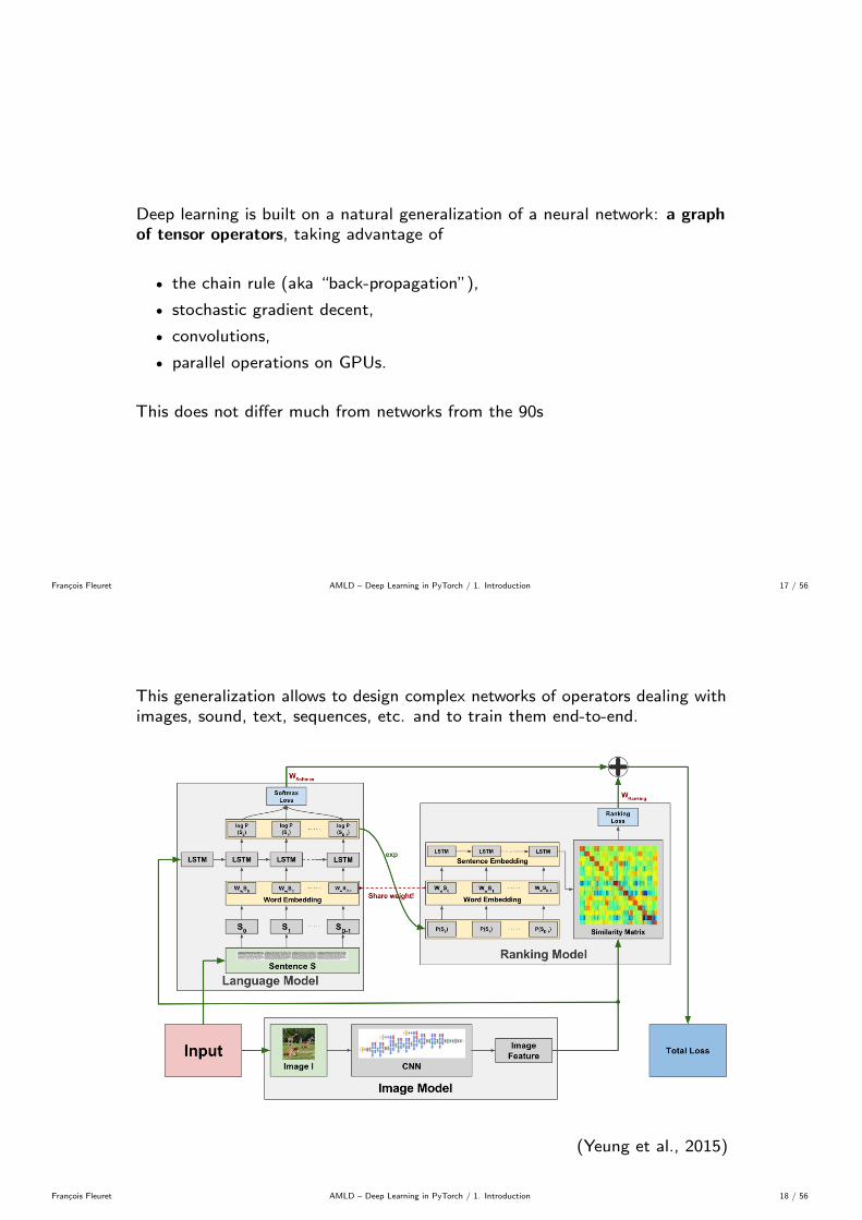
Deep learning is built on a natural generalization of a neural network: a graphof tensor operators, taking advantage of

• the chain rule (aka “back-propagation”),

• stochastic gradient decent,

• convolutions,

• parallel operations on GPUs.

This does not differ much from networks from the 90s


This generalization allows to design complex networks of operators dealing withimages, sound, text, sequences, etc. and to train them end-to-end.

(Yeung et al., 2015)


CIFAR10

32× 32 color images, 50k train samples, 10k test samples.

(Krizhevsky, 2009, chap. 3)


Performance on CIFAR10

75

80

85

90

95

100

2010 2012 2014 2016 2018

Krizhevsky et al. (2012)

Graham (2015)

Human performance

Real et al. (2018)

Acc

ura

cy (

%)

Year


model top-1 err. top-5 err.

VGG-16 [41] 28.07 9.33GoogLeNet [44] - 9.15PReLU-net [13] 24.27 7.38

plain-34 28.54 10.02ResNet-34 A 25.03 7.76ResNet-34 B 24.52 7.46ResNet-34 C 24.19 7.40ResNet-50 22.85 6.71ResNet-101 21.75 6.05ResNet-152 21.43 5.71

Table 3. Error rates (%, 10-crop testing) on ImageNet validation.VGG-16 is based on our test. ResNet-50/101/152 are of option Bthat only uses projections for increasing dimensions.

method top-1 err. top-5 err.

VGG [41] (ILSVRC’14) - 8.43†

GoogLeNet [44] (ILSVRC’14) - 7.89VGG [41] (v5) 24.4 7.1PReLU-net [13] 21.59 5.71BN-inception [16] 21.99 5.81ResNet-34 B 21.84 5.71ResNet-34 C 21.53 5.60ResNet-50 20.74 5.25ResNet-101 19.87 4.60ResNet-152 19.38 4.49

Table 4. Error rates (%) of single-model results on the ImageNetvalidation set (except † reported on the test set).

method top-5 err. (test)VGG [41] (ILSVRC’14) 7.32GoogLeNet [44] (ILSVRC’14) 6.66VGG [41] (v5) 6.8PReLU-net [13] 4.94BN-inception [16] 4.82ResNet (ILSVRC’15) 3.57

Table 5. Error rates (%) of ensembles. The top-5 error is on thetest set of ImageNet and reported by the test server.

ResNet reduces the top-1 error by 3.5% (Table 2), resultingfrom the successfully reduced training error (Fig. 4 right vs.left). This comparison verifies the effectiveness of residuallearning on extremely deep systems.

Last, we also note that the 18-layer plain/residual netsare comparably accurate (Table 2), but the 18-layer ResNetconverges faster (Fig. 4 right vs. left). When the net is “notoverly deep” (18 layers here), the current SGD solver is stillable to find good solutions to the plain net. In this case, theResNet eases the optimization by providing faster conver-gence at the early stage.

Identity vs. Projection Shortcuts. We have shown that

3x3, 64

1x1, 64

relu

1x1, 256

relu

relu

3x3, 64

3x3, 64

relu

relu

64-d 256-d

Figure 5. A deeper residual function F for ImageNet. Left: abuilding block (on 56×56 feature maps) as in Fig. 3 for ResNet-34. Right: a “bottleneck” building block for ResNet-50/101/152.

parameter-free, identity shortcuts help with training. Nextwe investigate projection shortcuts (Eqn.(2)). In Table 3 wecompare three options: (A) zero-padding shortcuts are usedfor increasing dimensions, and all shortcuts are parameter-free (the same as Table 2 and Fig. 4 right); (B) projec-tion shortcuts are used for increasing dimensions, and othershortcuts are identity; and (C) all shortcuts are projections.

Table 3 shows that all three options are considerably bet-ter than the plain counterpart. B is slightly better than A. Weargue that this is because the zero-padded dimensions in Aindeed have no residual learning. C is marginally better thanB, and we attribute this to the extra parameters introducedby many (thirteen) projection shortcuts. But the small dif-ferences among A/B/C indicate that projection shortcuts arenot essential for addressing the degradation problem. So wedo not use option C in the rest of this paper, to reduce mem-ory/time complexity and model sizes. Identity shortcuts areparticularly important for not increasing the complexity ofthe bottleneck architectures that are introduced below.

Deeper Bottleneck Architectures. Next we describe ourdeeper nets for ImageNet. Because of concerns on the train-ing time that we can afford, we modify the building blockas a bottleneck design4. For each residual function F , weuse a stack of 3 layers instead of 2 (Fig. 5). The three layersare 1×1, 3×3, and 1×1 convolutions, where the 1×1 layersare responsible for reducing and then increasing (restoring)dimensions, leaving the 3×3 layer a bottleneck with smallerinput/output dimensions. Fig. 5 shows an example, whereboth designs have similar time complexity.

The parameter-free identity shortcuts are particularly im-portant for the bottleneck architectures. If the identity short-cut in Fig. 5 (right) is replaced with projection, one canshow that the time complexity and model size are doubled,as the shortcut is connected to the two high-dimensionalends. So identity shortcuts lead to more efficient modelsfor the bottleneck designs.

50-layer ResNet: We replace each 2-layer block in the

4Deeper non-bottleneck ResNets (e.g., Fig. 5 left) also gain accuracyfrom increased depth (as shown on CIFAR-10), but are not as economicalas the bottleneck ResNets. So the usage of bottleneck designs is mainly dueto practical considerations. We further note that the degradation problemof plain nets is also witnessed for the bottleneck designs.

6

(He et al., 2015)


Current application domains


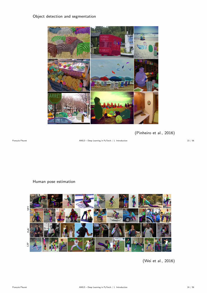
Object detection and segmentation

16 Pinheiro, Lin, Collobert, Dollar

Fig. 8: More selected qualitative results (see also Figure 4).

(Pinheiro et al., 2016)


Human pose estimation

(Wei et al., 2016)


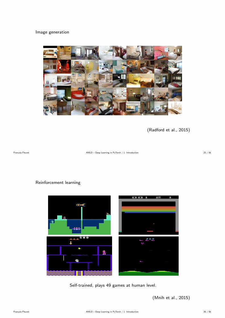
Image generation

(Radford et al., 2015)


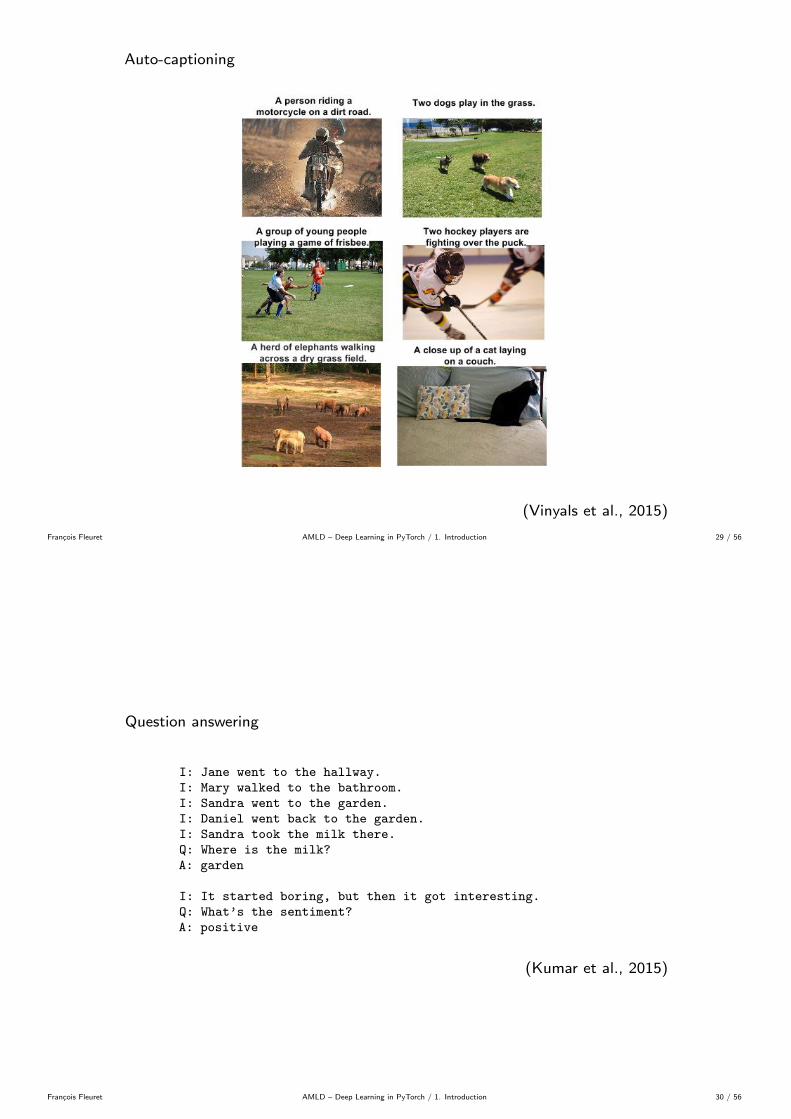
Reinforcement learning

Self-trained, plays 49 games at human level.

(Mnih et al., 2015)


Strategy games

March 2016, 4-1 against a 9-dan professional without handicap.

(Silver et al., 2016)


Translation

“The reason Boeing are doing this is to cram more seats in to make their planemore competitive with our products,” said Kevin Keniston, head of passengercomfort at Europe’s Airbus.

Ù“La raison pour laquelle Boeing fait cela est de creer plus de sieges pour rendreson avion plus competitif avec nos produits”, a declare Kevin Keniston, chefdu confort des passagers chez Airbus.

When asked about this, an official of the American administration replied:“The United States is not conducting electronic surveillance aimed at officesof the World Bank and IMF in Washington.”

ÙInterroge a ce sujet, un fonctionnaire de l’administration americaine a repondu:“Les Etats-Unis n’effectuent pas de surveillance electronique a l’intention desbureaux de la Banque mondiale et du FMI a Washington”

(Wu et al., 2016)


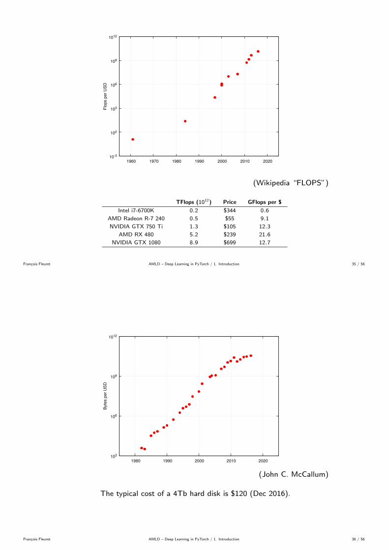
Auto-captioning

Figure 5. A selection of evaluation results, grouped by human rating.

4.3.7 Analysis of Embeddings

In order to represent the previous word St−1 as input tothe decoding LSTM producing St, we use word embeddingvectors [22], which have the advantage of being indepen-dent of the size of the dictionary (contrary to a simpler one-hot-encoding approach). Furthermore, these word embed-dings can be jointly trained with the rest of the model. Itis remarkable to see how the learned representations havecaptured some semantic from the statistics of the language.Table 4.3.7 shows, for a few example words, the nearestother words found in the learned embedding space.

Note how some of the relationships learned by the modelwill help the vision component. Indeed, having “horse”,“pony”, and “donkey” close to each other will encourage theCNN to extract features that are relevant to horse-lookinganimals. We hypothesize that, in the extreme case wherewe see very few examples of a class (e.g., “unicorn”), itsproximity to other word embeddings (e.g., “horse”) shouldprovide a lot more information that would be completelylost with more traditional bag-of-words based approaches.

5. Conclusion

We have presented NIC, an end-to-end neural networksystem that can automatically view an image and generate

Word Neighborscar van, cab, suv, vehicule, jeepboy toddler, gentleman, daughter, sonstreet road, streets, highway, freewayhorse pony, donkey, pig, goat, mulecomputer computers, pc, crt, chip, compute

Table 6. Nearest neighbors of a few example words

a reasonable description in plain English. NIC is based ona convolution neural network that encodes an image into acompact representation, followed by a recurrent neural net-work that generates a corresponding sentence. The model istrained to maximize the likelihood of the sentence given theimage. Experiments on several datasets show the robust-ness of NIC in terms of qualitative results (the generatedsentences are very reasonable) and quantitative evaluations,using either ranking metrics or BLEU, a metric used in ma-chine translation to evaluate the quality of generated sen-tences. It is clear from these experiments that, as the sizeof the available datasets for image description increases, sowill the performance of approaches like NIC. Furthermore,it will be interesting to see how one can use unsuperviseddata, both from images alone and text alone, to improve im-age description approaches.

(Vinyals et al., 2015)


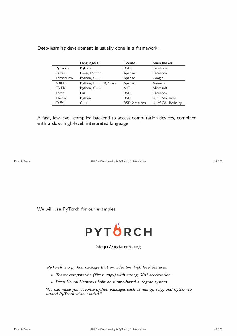
Question answering

I: Jane went to the hallway.I: Mary walked to the bathroom.I: Sandra went to the garden.I: Daniel went back to the garden.I: Sandra took the milk there.Q: Where is the milk?A: garden

I: It started boring, but then it got interesting.Q: What’s the sentiment?A: positive

(Kumar et al., 2015)


Why does it work now?


The success of deep learning is multi-factorial:

• Five decades of research in machine learning,

• CPUs/GPUs/storage developed for other purposes,

• lots of data from “the internet”,

• tools and culture of collaborative and reproducible science,

• resources and efforts from large corporations.


Five decades of research in ML provided

• a taxonomy of ML concepts (classification, generative models, clustering,kernels, linear embeddings, etc.),

• a sound statistical formalization (Bayesian estimation, PAC),

• a clear picture of fundamental issues (bias/variance dilemma, VCdimension, generalization bounds, etc.),

• a good understanding of optimization issues,

• efficient large-scale algorithms.


From a practical perspective, deep learning

• lessens the need for a deep mathematical grasp,

• makes the design of large learning architectures a system/softwaredevelopment task,

• allows to leverage modern hardware (clusters of GPUs),

• does not plateau when using more data,

• makes large trained networks a commodity.


10-3

100

103

106

109

1012

1960 1970 1980 1990 2000 2010 2020

Flop

s pe

r US

D

(Wikipedia “FLOPS”)

TFlops (1012) Price GFlops per $

Intel i7-6700K 0.2 $344 0.6

AMD Radeon R-7 240 0.5 $55 9.1

NVIDIA GTX 750 Ti 1.3 $105 12.3

AMD RX 480 5.2 $239 21.6

NVIDIA GTX 1080 8.9 $699 12.7


103

106

109

1012

1980 1990 2000 2010 2020

Byt

es p

er U

SD

(John C. McCallum)

The typical cost of a 4Tb hard disk is $120 (Dec 2016).


AlexNet

BN-AlexNet

BN-NIN

GoogLeNet

ResNet-1

8

VGG-16

VGG-19

ResNet-3

4

ResNet-5

0

ResNet-1

01

Inception-v3

50

55

60

65

70

75

80

Top-1

acc

ura

cy [

%]

0 5 10 15 20 25 30 35 40

Operations [G-Ops]

50

55

60

65

70

75

80Top-1

acc

ura

cy [

%]

AlexNetBN-AlexNet

BN-NIN

ResNet-18

VGG-16 VGG-19

GoogLeNet

ResNet-34

ResNet-50ResNet-101

Inception-v3

5M 35M 65M 95M 125M 155M

Figure 1: Top1 vs. network. Single-crop top-1 vali-dation accuracies for top scoring single-model archi-tectures. We introduce with this chart our choice ofcolour scheme, which will be used throughout thispublication to distinguish effectively different archi-tectures and their correspondent authors. Notice thatnetwork of the same group share colour, for exampleResNet are all variations of pink.

Figure 2: Top1 vs. operations, size ∝ parameters.Top-1 one-crop accuracy versus amount of operationsrequired for a single forward pass. The size of theblobs is proportional to the number of network param-eters; a legend is reported in the bottom right corner,spanning from 5× 106 to 155× 106 params.

1 2 4 8 16 32 64

Batch size [ / ]

0

100

200

300

400

500

600

Fow

ard

tim

e p

er

image [

ms]

BN-NIN

GoogLeNet

Inception-v3

AlexNet

BN-AlexNet

VGG-16

VGG-19

ResNet-18

ResNet-34

ResNet-50

ResNet-101

1 2 4 8 16 32 64

Batch size [ / ]

5

10

20

50

100

200

500

Fow

ard

tim

e p

er

image [

ms]

BN-NIN

GoogLeNet

Inception-v3

AlexNet

BN-AlexNet

VGG-16

VGG-19

ResNet-18

ResNet-34

ResNet-50

ResNet-101

Figure 3: Inference time vs. batch size. These two charts show inference time across different batch sizes witha linear and logarithmic ordinate respectively and logarithmic abscissa. Missing data points are due to lack ofenough system memory required to process bigger batches.

3.2 Inference Time

Figure 3 reports inference time per image on each architecture, as a function of image batch size(from 1 to 64). We notice that VGG processes one image in more than half second, making it a lesslikely contender in real-time applications on a NVIDIA TX1. AlexNet shows a speed up of roughly15× going from batch of 1 to 64 images, due to weak optimisation of its fully connected layers. It isa very surprising finding, that will be further discussed in the next subsection.

3.3 Power

Power measurements are complicated by the high frequency swings in current consumption, whichrequired high sampling current read-out to avoid aliasing. In this work, we used a 200MHz digitaloscilloscope with a current probe, as reported in section 2. Other measuring instruments, such as anAC power strip with 2Hz sampling rate, or a GPIB controlled DC power supply with 12Hz samplingrate, did not provide enough bandwidth to properly conduct power measurements.

3

(Canziani et al., 2016)


Implementing a deep network, PyTorch


Deep-learning development is usually done in a framework:

Language(s) License Main backer

PyTorch Python BSD Facebook

Caffe2 C++, Python Apache Facebook

TensorFlow Python, C++ Apache Google

MXNet Python, C++, R, Scala Apache Amazon

CNTK Python, C++ MIT Microsoft

Torch Lua BSD Facebook

Theano Python BSD U. of Montreal

Caffe C++ BSD 2 clauses U. of CA, Berkeley

A fast, low-level, compiled backend to access computation devices, combinedwith a slow, high-level, interpreted language.


We will use PyTorch for our examples.

http://pytorch.org

“PyTorch is a python package that provides two high-level features:

• Tensor computation (like numpy) with strong GPU acceleration

• Deep Neural Networks built on a tape-based autograd system

You can reuse your favorite python packages such as numpy, scipy and Cython toextend PyTorch when needed.”


http://pytorch.org

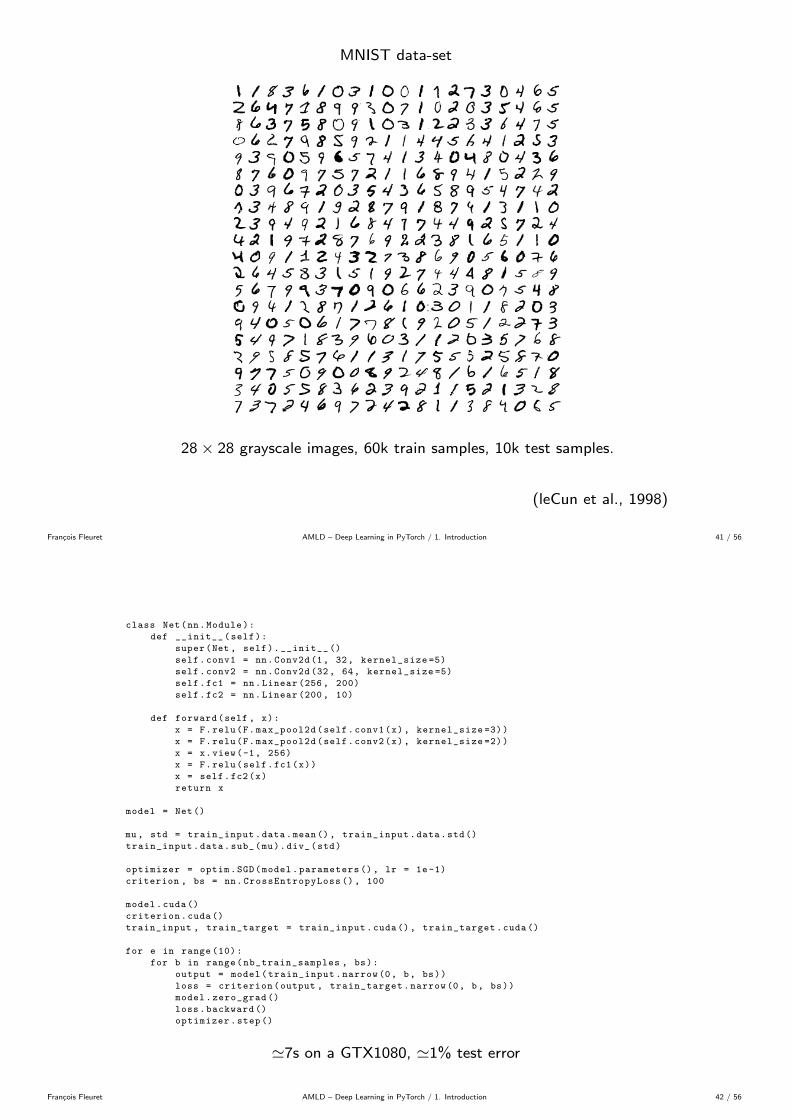
MNIST data-set

28× 28 grayscale images, 60k train samples, 10k test samples.

(leCun et al., 1998)


class Net(nn.Module):

def __init__(self):

super(Net , self).__init__ ()

self.conv1 = nn.Conv2d(1, 32, kernel_size =5)

self.conv2 = nn.Conv2d (32, 64, kernel_size =5)

self.fc1 = nn.Linear (256, 200)

self.fc2 = nn.Linear (200, 10)

def forward(self , x):

x = F.relu(F.max_pool2d(self.conv1(x), kernel_size =3))

x = F.relu(F.max_pool2d(self.conv2(x), kernel_size =2))

x = x.view(-1, 256)

x = F.relu(self.fc1(x))

x = self.fc2(x)

return x

model = Net()

mu , std = train_input.data.mean(), train_input.data.std()

train_input.data.sub_(mu).div_(std)

optimizer = optim.SGD(model.parameters (), lr = 1e-1)

criterion , bs = nn.CrossEntropyLoss (), 100

model.cuda()

criterion.cuda()

train_input , train_target = train_input.cuda(), train_target.cuda()

for e in range (10):

for b in range(nb_train_samples , bs):

output = model(train_input.narrow(0, b, bs))

loss = criterion(output , train_target.narrow(0, b, bs))

model.zero_grad ()

loss.backward ()

optimizer.step()

'7s on a GTX1080, '1% test error


Learning from data


The general objective of machine learning is to capture regularity in data tomake predictions.

In our regression example, we modeled age and blood pressure as being linearlyrelated, to predict the latter from the former.

There are multiple types of inference that we can roughly split into threecategories:

• Classification (e.g. object recognition, cancer detection, speechprocessing),

• regression (e.g. customer satisfaction, stock prediction, epidemiology), and

• density estimation (e.g. outlier detection, data visualization,sampling/synthesis).


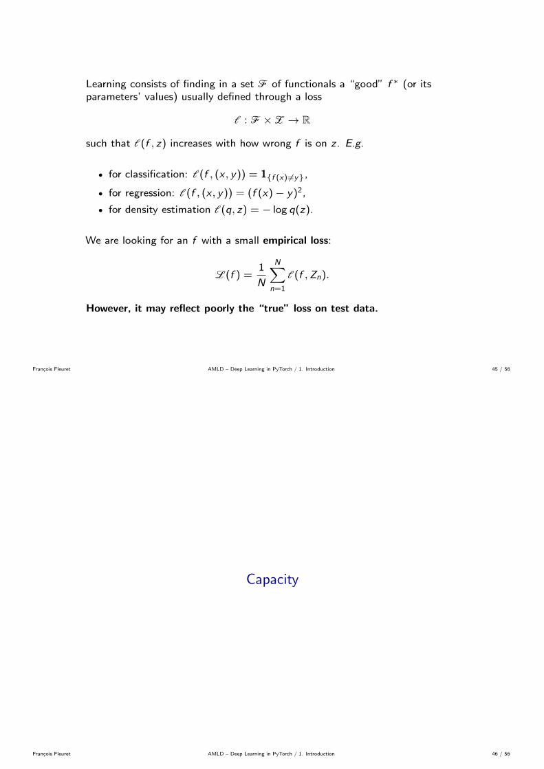
Learning consists of finding in a set F of functionals a “good” f ∗ (or itsparameters’ values) usually defined through a loss

l : F ×Z → R

such that l(f , z) increases with how wrong f is on z. E.g.

• for classification: l(f , (x , y)) = 1{f (x) 6=y},

• for regression: l(f , (x , y)) = (f (x)− y)2,

• for density estimation l(q, z) = − log q(z).

We are looking for an f with a small empirical loss:

L(f ) =1

N

N∑n=1

l(f ,Zn).

However, it may reflect poorly the “true” loss on test data.


Capacity


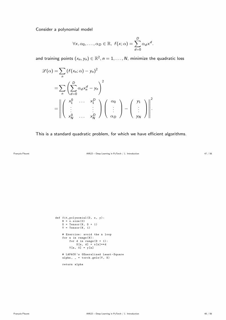
Consider a polynomial model

∀x , α0, . . . , αD ∈ R, f (x ;α) =D∑

d=0

αdxd .

and training points (xn, yn) ∈ R2, n = 1, . . . ,N, minimize the quadratic loss

L(α) =∑n

(f (xn;α)− yn)2

=∑n

(D∑

d=0

αdxdn − yn

)2

=

∥∥∥∥∥∥∥ x0

1 . . . xD1...

...x0N . . . xDN

α0

...αD

− y1

...yN

∥∥∥∥∥∥∥

2

.

This is a standard quadratic problem, for which we have efficient algorithms.


def fit_polynomial(D, x, y):

N = x.size (0)

X = Tensor(N, D + 1)

Y = Tensor(N, 1)

# Exercise: avoid the n loop

for n in range(N):

for d in range(D + 1):

X[n, d] = x[n]**d

Y[n, 0] = y[n]

# LAPACK ’s GEneralized Least -Square

alpha , _ = torch.gels(Y, X)

return alpha


-0.5

0

0.5

1

1.5

0 0.2 0.4 0.6 0.8 1

Data

-0.5

0

0.5

1

1.5

0 0.2 0.4 0.6 0.8 1

Degree D=0

Dataf*

-0.5

0

0.5

1

1.5

0 0.2 0.4 0.6 0.8 1

Degree D=1

Dataf*

-0.5

0

0.5

1

1.5

0 0.2 0.4 0.6 0.8 1

Degree D=2

Dataf*

-0.5

0

0.5

1

1.5

0 0.2 0.4 0.6 0.8 1

Degree D=3

Dataf*

-0.5

0

0.5

1

1.5

0 0.2 0.4 0.6 0.8 1

Degree D=4

Dataf*

-0.5

0

0.5

1

1.5

0 0.2 0.4 0.6 0.8 1

Degree D=5

Dataf*

-0.5

0

0.5

1

1.5

0 0.2 0.4 0.6 0.8 1

Degree D=6

Dataf*

-0.5

0

0.5

1

1.5

0 0.2 0.4 0.6 0.8 1

Degree D=7

Dataf*

-0.5

0

0.5

1

1.5

0 0.2 0.4 0.6 0.8 1

Degree D=8

Dataf*

-0.5

0

0.5

1

1.5

0 0.2 0.4 0.6 0.8 1

Degree D=9

Dataf*


We define the capacity of a set of predictors as its ability to model an arbitraryfunctional.

Although it is difficult to define precisely, it is quite clear in practice how toincrease or decrease it for a given class of models.

• If the capacity is too low, the predictor does not fit the data. The trainingerror is high, and reflects the test error.

⇒ Under-fitting.

• If the capacity is too high, the predictor fits well the data including noise.The training error is low, and does not reflect the test error.

⇒ Over-fitting.


Proper evaluation protocols


Learning algorithms, in particular deep-learning ones, require the tuning of manymeta-parameters.

These parameters have a strong impact on the performance, resulting in a“meta” over-fitting through experiments.

We must be extra careful with performance estimation.

Running 100 times our experiment on MNIST, with randomized weights, we get:

Worst Median Best1.3% 1.0% 0.82%


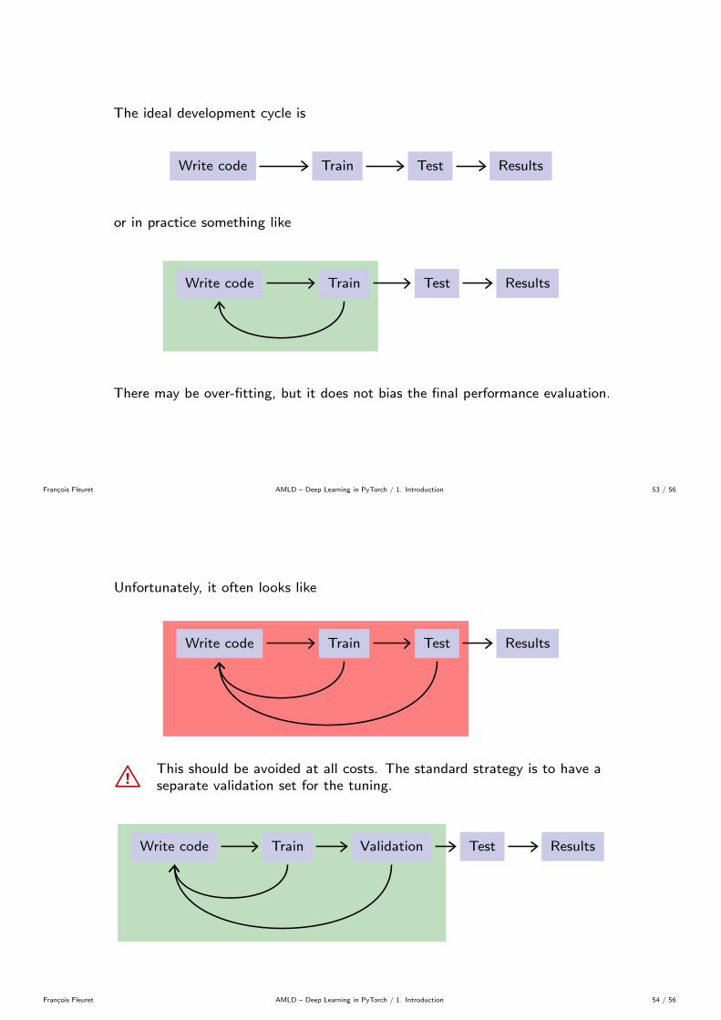
The ideal development cycle is

Write code Train Test Results

or in practice something like


There may be over-fitting, but it does not bias the final performance evaluation.


Unfortunately, it often looks like


B This should be avoided at all costs. The standard strategy is to have aseparate validation set for the tuning.

Write code Train Validation Test Results


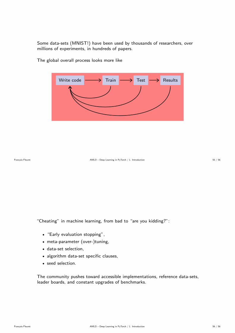
Some data-sets (MNIST!) have been used by thousands of researchers, overmillions of experiments, in hundreds of papers.

The global overall process looks more like



“Cheating” in machine learning, from bad to “are you kidding?”:

• “Early evaluation stopping”,

• meta-parameter (over-)tuning,

• data-set selection,

• algorithm data-set specific clauses,

• seed selection.

The community pushes toward accessible implementations, reference data-sets,leader boards, and constant upgrades of benchmarks.


References

A. Canziani, A. Paszke, and E. Culurciello. An analysis of deep neural network models forpractical applications. CoRR, abs/1605.07678, 2016.

K. Fukushima. Neocognitron: A self-organizing neural network model for a mechanism ofpattern recognition unaffected by shift in position. Biological Cybernetics, 36(4):193–202, April 1980.

K. He, X. Zhang, S. Ren, and J. Sun. Deep residual learning for image recognition. CoRR,abs/1512.03385, 2015.

A. Krizhevsky. Learning multiple layers of features from tiny images. Master’s thesis,Department of Computer Science, University of Toronto, 2009.

A. Krizhevsky, I. Sutskever, and G. Hinton. Imagenet classification with deep convolutionalneural networks. In Neural Information Processing Systems (NIPS), 2012.

A. Kumar, O. Irsoy, J. Su, J. Bradbury, R. English, B. Pierce, P. Ondruska, I. Gulrajani,and R. Socher. Ask me anything: Dynamic memory networks for natural languageprocessing. CoRR, abs/1506.07285, 2015.

Y. leCun, L. Bottou, Y. Bengio, and P. Haffner. Gradient-based learning applied todocument recognition. Proceedings of the IEEE, 86(11):2278–2324, 1998.

W. S. McCulloch and W. Pitts. A logical calculus of the ideas immanent in nervous activity.The bulletin of mathematical biophysics, 5(4):115–133, 1943.


V. Mnih, K. Kavukcuoglu, D. Silver, A. A. Rusu, J. Veness, M. G. Bellemare, A. Graves,M. Riedmiller, A. K. Fidjeland, G. Ostrovski, S. Petersen, C. Beattie, A. Sadik,I. Antonoglou, H. King, D. Kumaran, D. Wierstra, S. Legg, and D. Hassabis.Human-level control through deep reinforcement learning. Nature, 518(7540):529–533,Feb. 2015.

P. O. Pinheiro, T.-Y. Lin, R. Collobert, and P. Dollar. Learning to refine object segments.In European Conference on Computer Vision (ECCV), pages 75–91, 2016.

A. Radford, L. Metz, and S. Chintala. Unsupervised representation learning with deepconvolutional generative adversarial networks. CoRR, abs/1511.06434, 2015.

D. E. Rumelhart, G. E. Hinton, and R. J. Williams. Neurocomputing: Foundations ofResearch, chapter Learning Representations by Back-propagating Errors, pages 696–699.MIT Press, 1988.

D. Silver, A. Huang, C. J. Maddison, A. Guez, L. Sifre, G. van den Driessche,J. Schrittwieser, I. Antonoglou, V. Panneershelvam, M. Lanctot, S. Dieleman, D. Grewe,J. Nham, N. Kalchbrenner, I. Sutskever, T. Lillicrap, M. Leach, K. Kavukcuoglu,T. Graepel, and D. Hassabis. Mastering the game of go with deep neural networks andtree search. Nature, 529:484–503, 2016.

C. Szegedy, W. Liu, Y. Jia, P. Sermanet, S. Reed, D. Anguelov, D. Erhan, V. Vanhoucke,and A. Rabinovich. Going deeper with convolutions. In Conference on Computer Visionand Pattern Recognition (CVPR), 2015.

O. Vinyals, A. Toshev, S. Bengio, and D. Erhan. Show and tell: A neural image captiongenerator. In Conference on Computer Vision and Pattern Recognition (CVPR), 2015.

S. Wei, V. Ramakrishna, T. Kanade, and Y. Sheikh. Convolutional pose machines. CoRR,abs/1602.00134, 2016.


Y. Wu, M. Schuster, Z. Chen, Q. V. Le, M. Norouzi, W. Macherey, M. Krikun, Y. Cao,Q. Gao, K. Macherey, J. Klingner, A. Shah, M. Johnson, X. Liu, L. Kaiser, S. Gouws,Y. Kato, T. Kudo, H. Kazawa, K. Stevens, G. Kurian, N. Patil, W. Wang, C. Young,J. Smith, J. Riesa, A. Rudnick, O. Vinyals, G. Corrado, M. Hughes, and J. Dean.Google’s neural machine translation system: Bridging the gap between human andmachine translation. CoRR, abs/1609.08144, 2016.

S. Yeung, O. Russakovsky, G. Mori, and L. Fei-Fei. End-to-end learning of action detectionfrom frame glimpses in videos. CoRR, abs/1511.06984, 2015.


1. introduction amld { deep learning in pytorch · ì éiè"ä ì ûkè ç ï ï uÄ ï è©ì...

Documents