1 vector architectures sima, fountain and kacsuk chapter 14 cse462

1

VectorArchitectures

Sima, Fountain and KacsukChapter 14

CSE462

2

David Abramson, 2004 Material from Sima, Fountain and Kacsuk, Addison Wesley 1997

A Generic Vector Machine

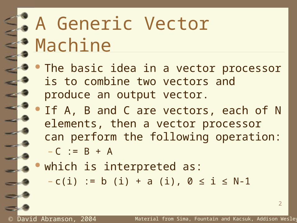
The basic idea in a vector processor is to combine two vectors and produce an output vector.

If A, B and C are vectors, each of N elements, then a vector processor can perform the following operation:– C := B + A

which is interpreted as:– c(i) := b (i) + a (i), 0 ≤ i ≤ N-1

3


A Generic Vector Processor

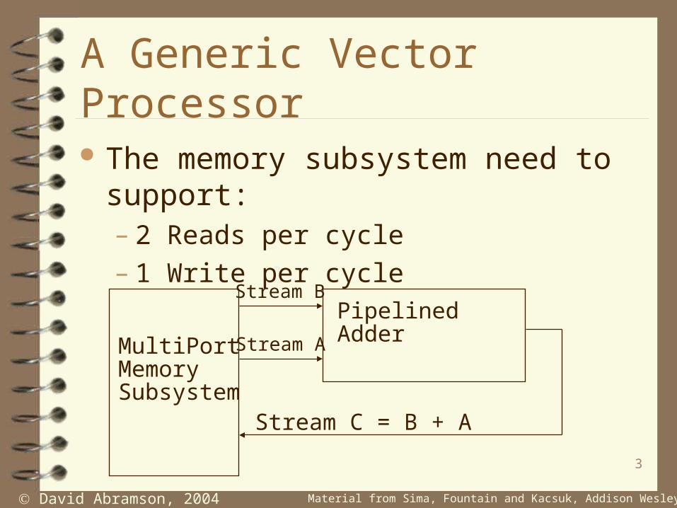
The memory subsystem need to support:– 2 Reads per cycle– 1 Write per cycle

MultiPortMemorySubsystem

Pipelined Adder

Stream B

Stream A

Stream C = B + A

4


Un-vectorized computation

Compute first address

Fetch first dataCompute second address

Fetch second data

Compute result

Fetch destination address

Store result

precomputetime t1

computetime t2

post-computetime t3

Time

Compute time for one result = t1 + t2 + t3

Compute time for N results = N(t1 + t2+ t3)

5


Vectorized computation


Fetch first dataCompute second address

Fetch second data

Compute resultFetch destination address

Store result

precomputetime t1

computetime t2

per result

post-computetime t3

Time

Compute time for N results = t1 + Nt2+ t3

6


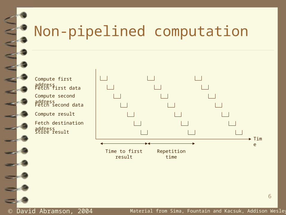
Non-pipelined computation


Fetch first data

Compute second address

Fetch second data

Compute result


Store result

Time

Time to first result Repetition time

7


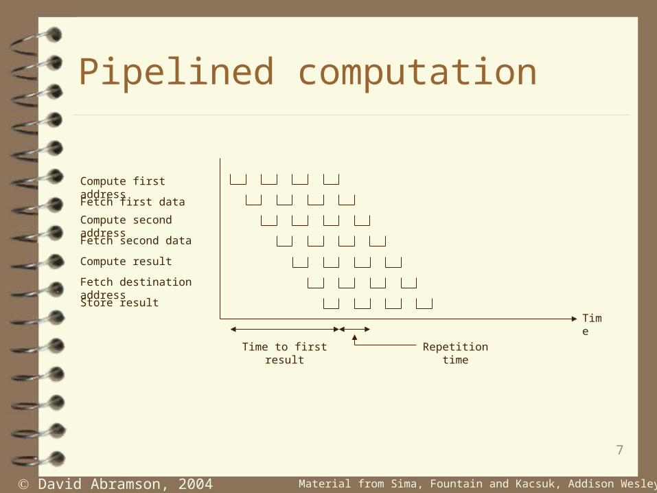
Pipelined computation


Fetch first data


Fetch second data

Compute result


Store result

Time


8


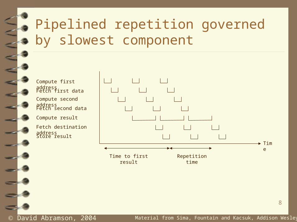
Pipelined repetition governed by slowest component


Fetch first data


Fetch second data

Compute result


Store result

Time


9


Pipelined granularity increased to improve repetition rate


Fetch first data


Fetch second data

Increased granularity for computation

Time


Store result


10


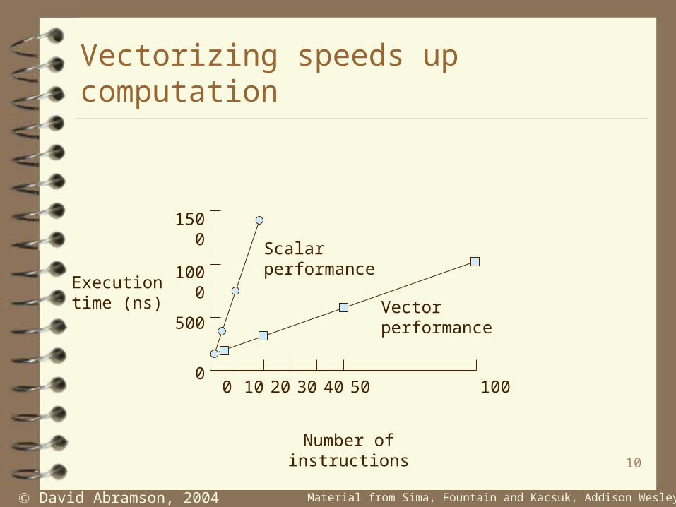
Vectorizing speeds up computation

1500

1000

500

0

Execution time (ns)

0 10 20 30 40 50 100

Number of instructions

Scalar performance

Vector performance

11


Interleaving

If vector pipelining is to work then it must be possible to fetch instructions from memory quickly.

There are two main ways of achieving this:– Cache Memories– Interleaving

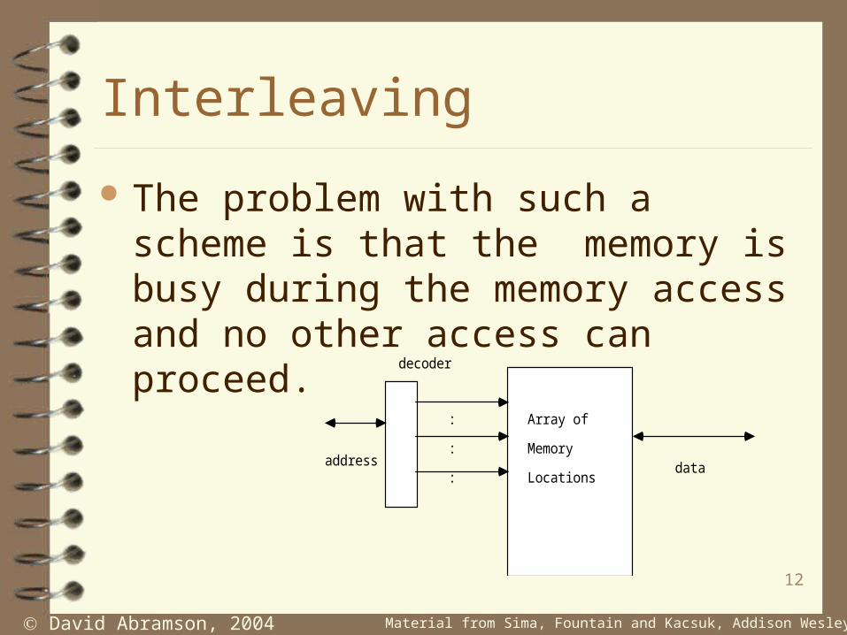
A conventional memory consists of a set of storage locations accessed via some sort of address decoder.

12


Interleaving

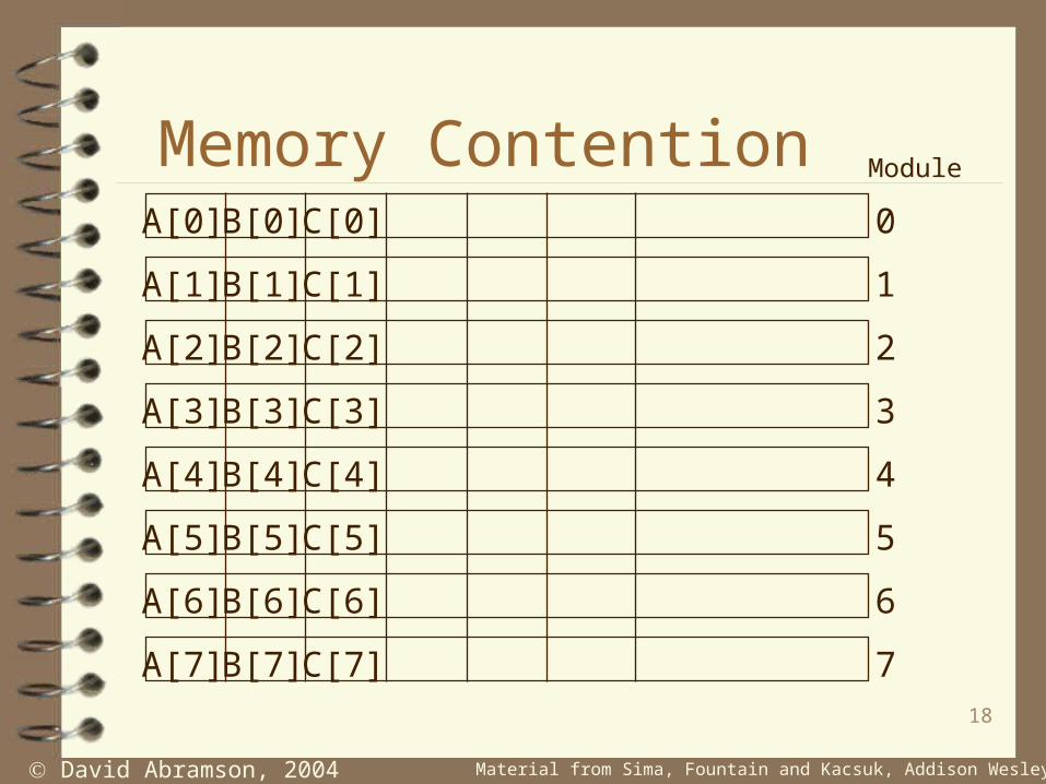
The problem with such a scheme is that the memory is busy during the memory access and no other access can proceed.

Array of Memory Locations

: : :

decoder

address data

13


Interleaving

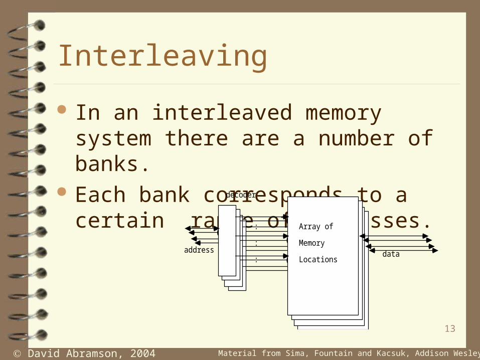
In an interleaved memory system there are a number of banks.

Each bank corresponds to a certain range of addresses.

Array of Memory Locations

: : :

decoder

address data

14


Interleaving

A pipelined machine can be kept fed with instructions even though the main memory may be quite slow.

An interleaved memory system slows down when subsequent accesses are for the same bank of memory.

Rare when prefetching instructions, because they tend to be sequential.

Possible to access two locations at the same time if they reside in different banks.

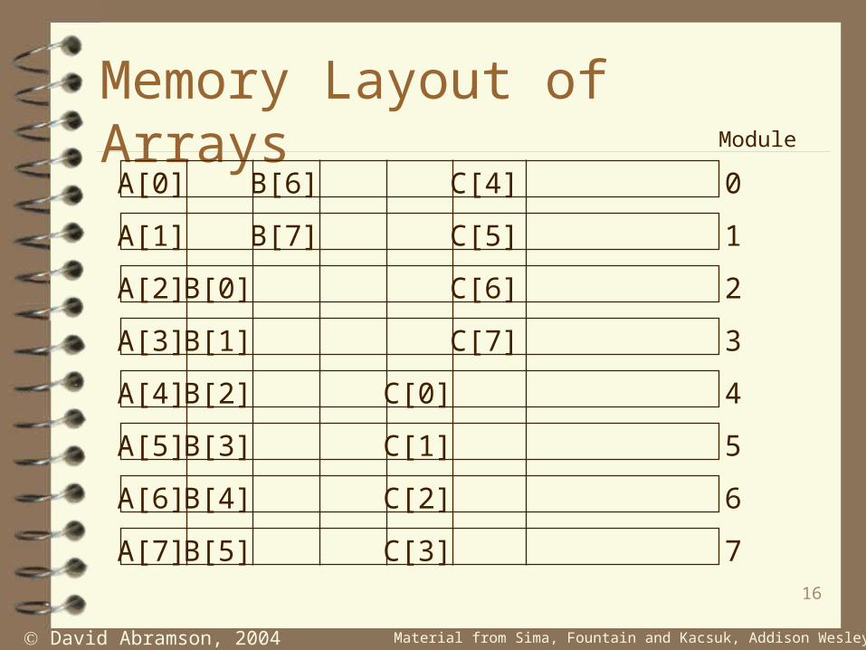
Banks are usually selected using some of the low order bits of the address because sequential access will access different banks.

15


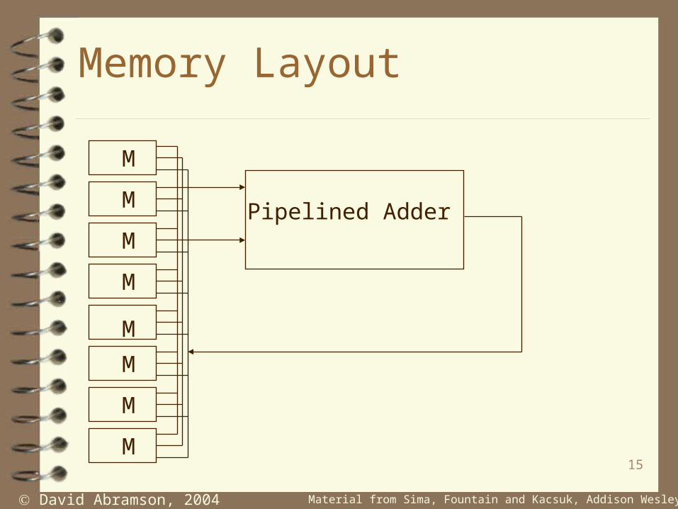
Memory Layout

M

M

M

M

M

M

M

M

Pipelined Adder

16


Memory Layout of Arrays

A[0]

A[1]

A[2]

A[3]

A[4]

A[5]

A[6]

A[7]

B[0]

B[1]

B[2]

B[3]

B[4]

B[5]

B[6]

B[7]

C[0]

C[1]

C[2]

C[3]

C[4]

C[5]

C[6]

C[7]

0

1

2

3

4

5

6

7

Module

17


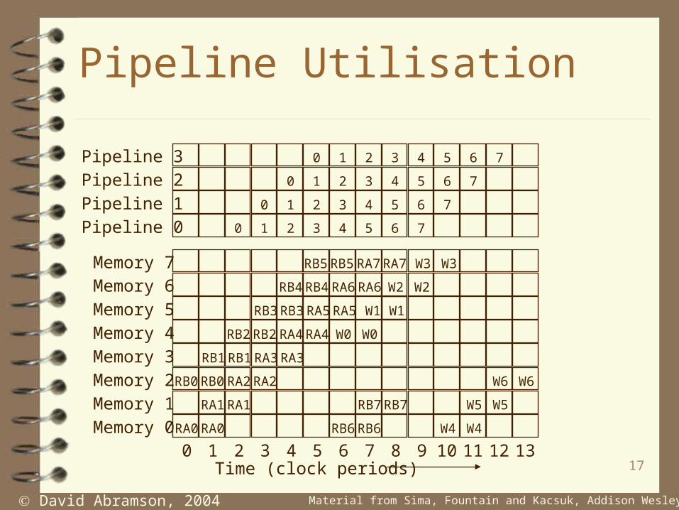
Pipeline Utilisation

Time (clock periods)0 1 2 3 4 5 6 7 8 9 10 11 12 13

Memory 0

Memory 1Memory 2Memory 3

Memory 4Memory 5

Memory 6Memory 7

Pipeline 0Pipeline 1


RA0RA0

RA1RA1

RA2RA2

RA3RA3

RA4RA4

RA5RA5

RA6RA6

RA7RA7

RB0RB0

RB1RB1

RB2 RB2

RB3 RB3

RB4 RB4

RB5RB5

RB6 RB6

RB7 RB7

0 1 2 3 4 5 6 7

0 1 2 3 4 5 6 7

0 1 2 3 4 5 6 7

0 1 2 3 4 5 6 7

W0 W0

W1 W1

W2 W2

W3 W3

W4 W4

W5 W5

W6 W6

18


Memory ContentionA[0]

A[1]

A[2]

A[3]

A[4]

A[5]

A[6]

A[7]

B[0]

B[1]

B[2]

B[3]

B[4]

B[5]

B[6]

B[7]

C[0]

C[1]

C[2]

C[3]

C[4]

C[5]

C[6]

C[7]

0

1

2

3

4

5

6

7

Module

19


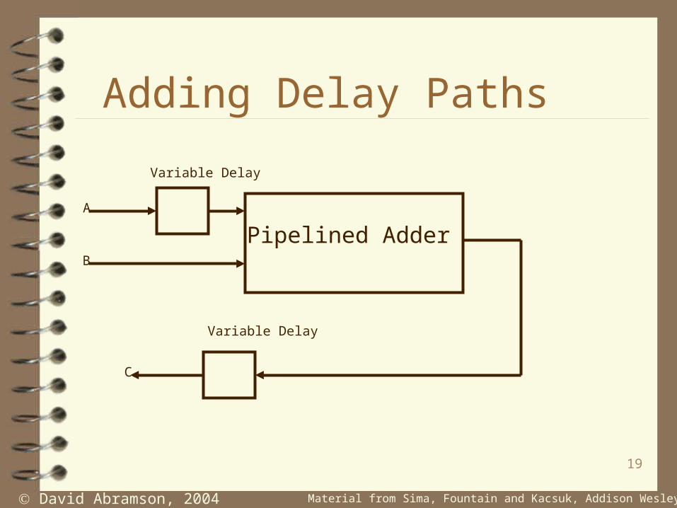
Adding Delay Paths

Pipelined Adder

Variable Delay

Variable Delay

A

B

C

20


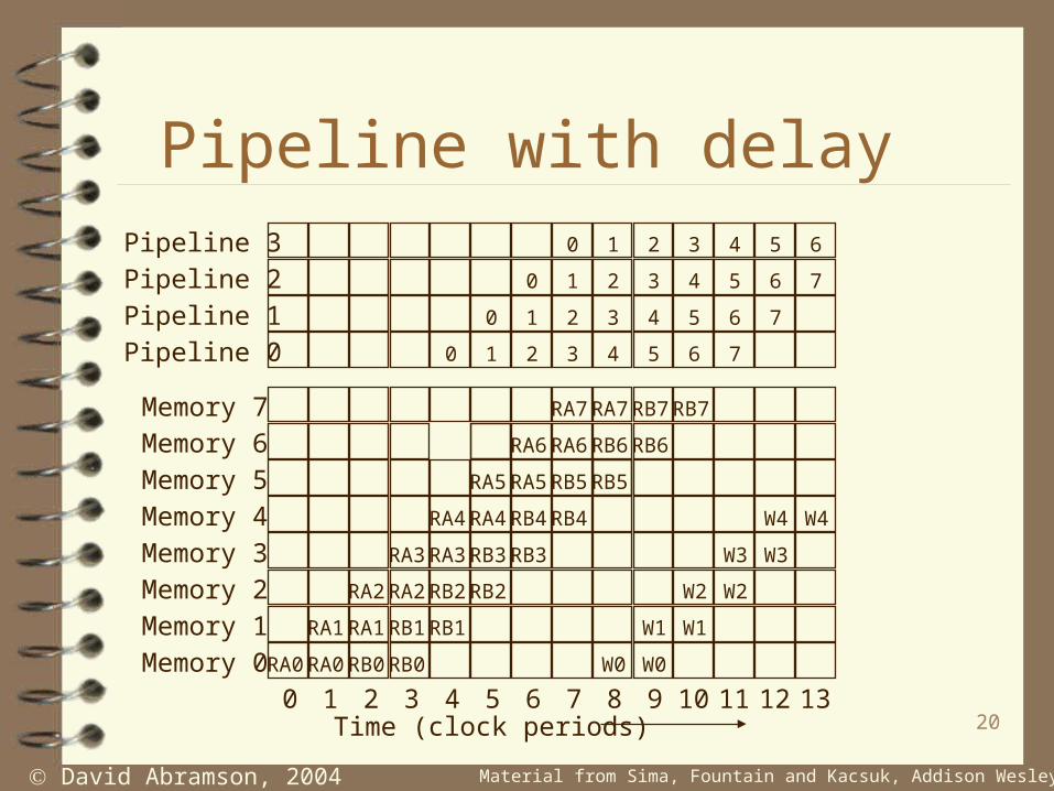
Pipeline with delay

Time (clock periods)0 1 2 3 4 5 6 7 8 9 10 11 12 13

Memory 0

Memory 1Memory 2Memory 3

Memory 4Memory 5

Memory 6Memory 7



RA0RA0

RA1RA1

RA2RA2

RA3RA3

RA4RA4

RA5RA5

RA6RA6

RA7RA7

RB0RB0

RB1RB1

RB2 RB2

RB3 RB3

RB4 RB4

RB5RB5

RB6 RB6

RB7 RB7

0 1 2 3 4 5 6 7

0 1 2 3 4 5 6 7

0 1 2 3 4 5 6 7

0 1 2 3 4 5 6

W0 W0

W1 W1

W2 W2

W3 W3

W4 W4

21


CRAY 1 Vector Operations

Vector facility The CRAY compilers are vectorising, and do not

require vector notation– do 10 i=1,64– 10 x(i) = y(i)

Scalar arithmetic – 64*n instructions, where n is the number of instructions per

loop iteration. Vector registers can also be sent to the floating point

functional units.

22


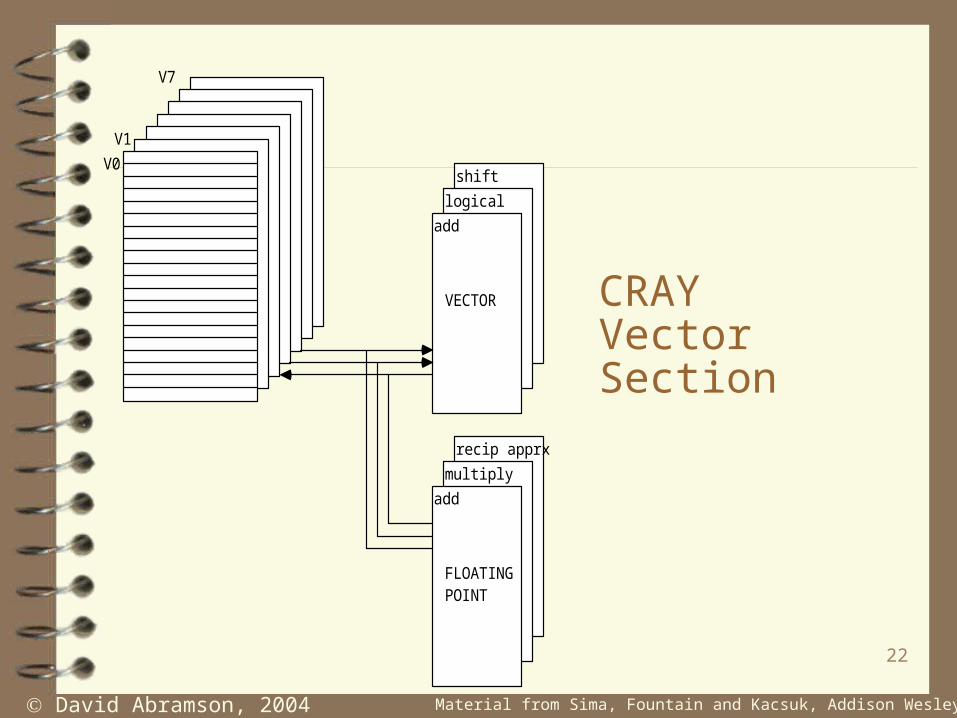
CRAY Vector Section

V0

V1

V7

VECTOR

add

logical

shift

FLOATING POINT

add

multiply

recip apprx

24


Chaining

The CRAY-1 can achieve even faster vector operations by using chaining.

Result vector is not only sent to the destination vector register, but also directly to another functional unit.

Data is seen to chain from one functional unit to another possibly without any intermediate storage.

25


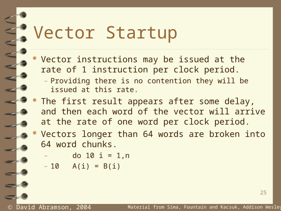
Vector Startup Vector instructions may be issued at the rate of 1

instruction per clock period. – Providing there is no contention they will be issued at this rate.

The first result appears after some delay, and then each word of the vector will arrive at the rate of one word per clock period.

Vectors longer than 64 words are broken into 64 word chunks.– do 10 i = 1,n

– 10 A(i) = B(i)

26


Vector Startup times

Note the second loop uses data chaining. Note the effect of startup time.

Loop Body 1 10 100 1000 Scalar 1000

A(i) = B(i) 44 5.8 2.7 2.5 31

A(i) = B(i)*C(i) + D(i)*E(i)

110 16 7.7 7.1 57

27


Effect of Stride on Interleaving

Most interleaving schemes simply take the bottom bits of the address and use these to select the memory bank.

This is very good for sequential address patterns (stride 1), and not too bad for random address patterns.

But for stride n, where n is the number of memory banks, the performance can be extremely bad.

DO 10 I = 1,128 DO 20 J = 1,12810 A(I,1) = 0 20 A(1,J) = 0

28


Effect of Stride

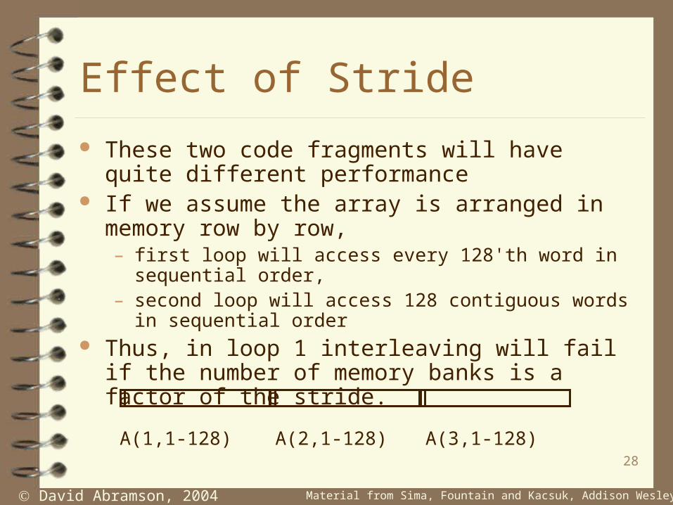
These two code fragments will have quite different performance

If we assume the array is arranged in memory row by row,– first loop will access every 128'th word in sequential order,– second loop will access 128 contiguous words in sequential order

Thus, in loop 1 interleaving will fail if the number of memory banks is a factor of the stride.

A(1,1-128) A(2,1-128) A(3,1-128)

29


Effect of Stride

Many research papers on how to improve the performance of stride m access on an n way interleaved memory system.

Two main approaches:– Arrange the data to match the stride (S/W)– Make the hardware insensitive to the stride

(H/W)

30


Memory Layout for stride free access

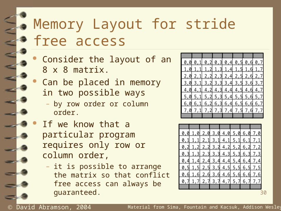
Consider the layout of an 8 x 8 matrix.

Can be placed in memory in two possible ways– by row order or column order.

If we know that a particular program requires only row or column order, – it is possible to arrange the matrix so

that conflict free access can always be guaranteed.

0,00,10,20,30,40,50,60,7

1,01,11,21,31,41,51,61,7

2,02,12,22,32,42,52,62,7

3,03,13,23,33,43,53,63,7

4,04,14,24,34,44,54,64,7

5,05,15,25,35,45,55,65,7

6,06,16,26,36,46,56,66,7

7,07,17,27,37,47,57,67,7

0,01,02,03,04,05,06,07,0

0,11,12,13,14,15,16,17,1

0,21,22,23,24,25,26,27,2

0,31,32,33,34,35,36,37,3

0,41,42,43,44,45,46,47,4

0,51,52,53,54,55,56,57,5

0,61,62,63,64,65,66,67,6

0,71,72,73,74,75,76,77,7

31


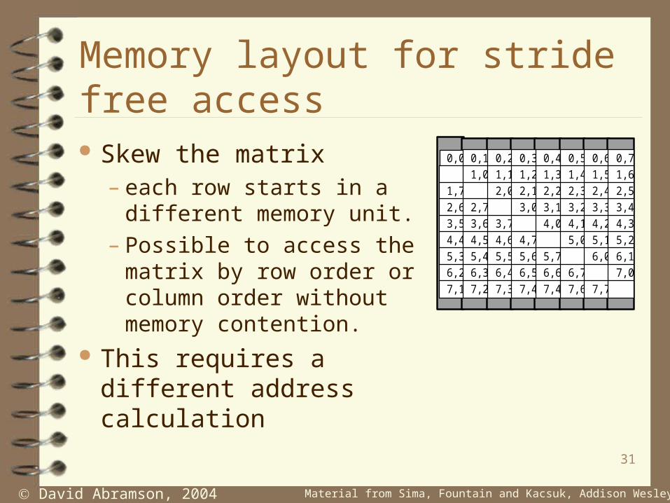
Memory layout for stride free access

Skew the matrix – each row starts in a different

memory unit. – Possible to access the matrix

by row order or column order without memory contention.

This requires a different address calculation

0,0

1,7

2,6

3,5

4,4

5,3

6,2

0,1

1,0

2,7

3,6

4,5

5,4

6,3

0,2

1,1

2,0

3,7

4,6

5,5

6,4

0,3

1,2

2,1

3,0

4,7

5,6

6,5

0,4

1,3

2,2

3,1

4,0

5,7

6,6

0,5

1,4

2,3

3,2

4,1

5,0

6,7

0,6

1,5

2,4

3,3

4,2

5,1

6,0

0,7

1,6

2,5

3,4

4,3

5,2

6,1

7,0

7,1 7,2 7,3 7,4 7,4 7,6 7,7

32


Address Modification in Hardware

Possible to use a different function to compute the module number.

If the address is passed to an arbitrary address computation function which emits a module number, – Produce stride free access for many different strides

There are schemes which give optimal packing and do not waste any space

33


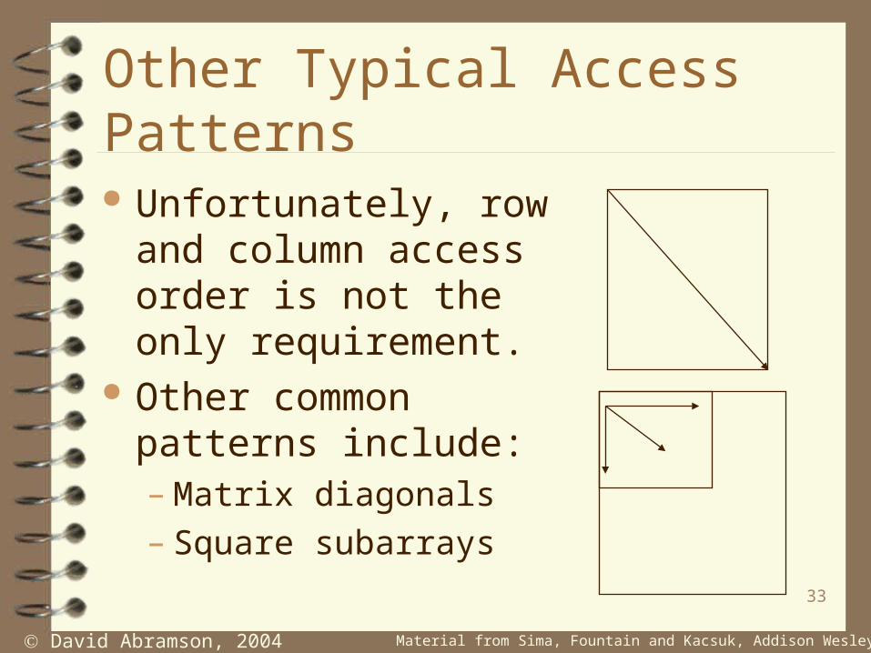
Other Typical Access Patterns

Unfortunately, row and column access order is not the only requirement.

Other common patterns include:– Matrix diagonals– Square subarrays

34


Diagonal Access

To access diagonal, – stride is equal to column stride + 1

If M, the number of modules isequal to power of 2, – both column stride and column stride +1 cannot

both be efficient, – both cannot be relatively prime to M.

35


Vector Algorithms

Consider the solution of the linear equations given by:– Ax = b

• A is an NxN matrix and

• x and b are N x 1 column vectors.

Gaussian Elimination is an efficient algorithm for producing upper and lower diagonal matrices L and U, such that– A = LU

36


Gaussian Elimination

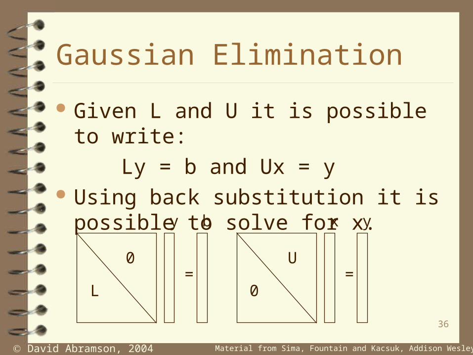
Given L and U it is possible to write:

Ly = b and Ux = y Using back substitution it is possible to

solve for x.

=L

0

y b

=0

U

x y

37


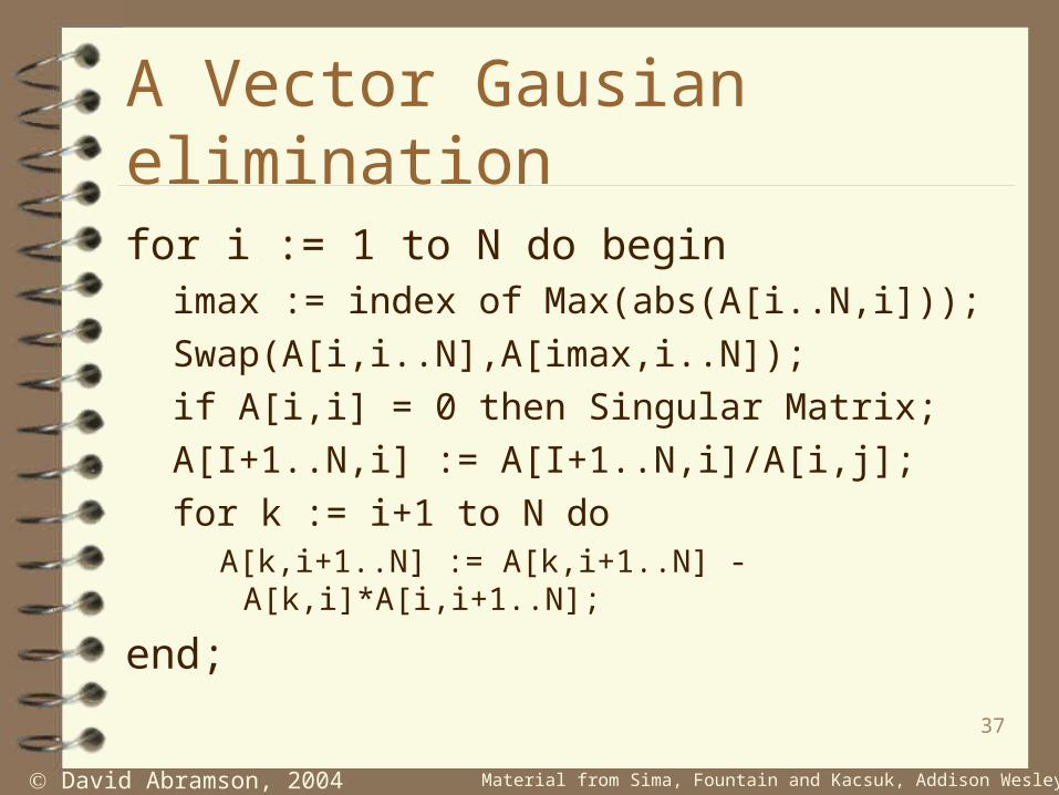
A Vector Gausian elimination

for i := 1 to N do beginimax := index of Max(abs(A[i..N,i]));

Swap(A[i,i..N],A[imax,i..N]);

if A[i,i] = 0 then Singular Matrix;

A[I+1..N,i] := A[I+1..N,i]/A[i,j];

for k := i+1 to N doA[k,i+1..N] := A[k,i+1..N] - A[k,i]*A[i,i+1..N];

end;

38


Picture of algorithm

U

LP U'

L' A

The algorithm produces a new row of U and column of L each iteration

39


Aspects of the algorithm

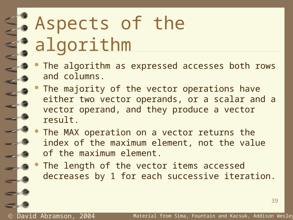
The algorithm as expressed accesses both rows and columns.

The majority of the vector operations have either two vector operands, or a scalar and a vector operand, and they produce a vector result.

The MAX operation on a vector returns the index of the maximum element, not the value of the maximum element.

The length of the vector items accessed decreases by 1 for each successive iteration.

40


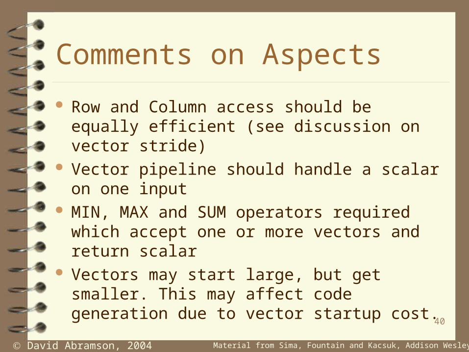
Comments on Aspects

Row and Column access should be equally efficient (see discussion on vector stride)

Vector pipeline should handle a scalar on one input

MIN, MAX and SUM operators required which accept one or more vectors and return scalar

Vectors may start large, but get smaller. This may affect code generation due to vector startup cost.

41


Sparse Matrices

In many engineering computations, there may be very large matrices. – May also be sparsely occupied, – Contain many zero elements.

Problems with the normal method of storing the matrix:– Occupy far too much memory– Very slow to process

42


Sparse Matrices ...

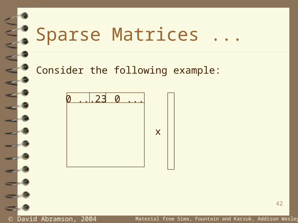
Consider the following example:

x

23 0 ...0 ...

43


Sparse Matrices ...

Many packages solve the problem by using a software data representation.– The trick is not to store the elements which

have zero values. At least two sorts of access mechanism:

– Random– Row/Column sequential.

44


Sparse Matrices ...

Matrix multiplication then consists of moving down the row/column pointers and multiplying elements of they have the same index values.

Hardware to implement this type of data representation.

Row Pointers

Column Pointers

1 vector architectures sima, fountain and kacsuk chapter 14 cse462

Documents

time compute time

address fetch

result post compute

result repetition time

resultrepetition time

addison wesley

david abramson

repetition rate compute