10 simulated response of avian biodiversity to biomass ... · simulated response of avian...

2016 Billion-Ton Report | 367

10 Simulated Response of Avian Biodiversity to Biomass Production

Henriette Jager,1 Gangsheng Wang,1 Jasmine Kreig,1 Nathan Sutton,1 and Ingrid Busch1

1 Oak Ridge National Laboratory

SimulAted ReSPonSe of AviAn BiodiveRSity to BiomASS PRoduction

368 | 2016 Billion-Ton Report

10.1 IntroductionCompared with other environmental indicators, few U.S. studies have quantified the relationships between pro-duction of biomass crops and biodiversity. The two are linked by both direct and indirect causal pathways. Indi-rectly, a growing bioenergy industry can delay or prevent bioclimatic stress (Cook, Beyea, and Keeler 1991a, b) to wildlife by replacing fossil energy and slowing the rate of climate warming (Dale, Parish, and Kline 2015). This is particularly true for ectotherms, including fish and other aquatic biota (Fenoglio et al. 2010). However, most public concerns center on direct linkages—specifically, how changes in land management to grow biomass will influence biodiversity. Here, we address this question, with a focus on birds that can be expanded to include other taxa in future assessments.

Public concern regarding biomass and its impact on biodiversity has been greatest in the Midwest, where 70% of diverse prairie and wetland ecosystems have been replaced by less-diverse agricultural landscapes (Samson, Knopf, and Ostlie 2004). This negative response in diversity to past changes in land management has taught us that replacing low-intensity, high-diversity land management with high-intensity, low-diversity land manage-ment is often accompanied by a reduction in species diversity (Meehan, Hurlbert, and Gratton 2010) and adds to public concern about increasing the agricultural footprint by adding biomass feedstock production. The expan-sion of corn grown for ethanol has also been raised as a concern for biodiversity (Brooke et al. 2009, Rashford, Walker, and Bastian 2011). However, biomass production can involve wildlife-friendly crops that mimic local native habitat (grasses and short-rotation woody crops [SRWCs]), crops that provide food (e.g., oil-seed crops for biodiesel), and more-intensive use (residue harvest) of existing croplands without expanding into less-man-aged land.

The analysis presented in this chapter builds on previous research. Many national-scale studies have quanti-fied future changes in wildlife habitat, for example, in response to changes in land cover (Tavernia et al. 2013, Lawler et al. 2014) or climate change [e.g., (Matthews et al. 2011)], but few studies have considered introduc-ing biomass feedstocks into future landscapes. In addition, many large-scale conservation-planning studies that assess the impacts of land-use change assume that all change is bad (Ando 1998, Withey et al. 2012). We relaxed this assumption by explicitly accounting for the value of biomass crops as wildlife habitat. Our approach was inspired, in part, by two earlier studies at the University of California, Berkeley. Both employed spatial optimi-zation to determine the best places to grow bioenergy crops for wildlife and for farmer profit. In a national-scale modeling study, the number of species of concern potentially impacted by replacing pasture with perennial grasses did not increase with increased farmer profit (Evans, Kelley, and Potts 2015). However, a trade-off be-tween biodiversity and farmer profit was evident when biomass was simulated on lands enrolled in the U.S. De-partment of Agriculture (USDA) Conservation Reserve Program (CRP lands) (Evans, Kelley, and Potts 2015). This study included 322 at-risk vertebrate species known to occupy cropland or grassland habitat. Evans, Kelley, and Potts estimated that 57 avian species might be influenced by conversion of cropland or pasture under a low-demand scenario (7.6 billion liters of fuel) and 119 species might be influenced under a high-demand (22.7 billion liters) scenario. They estimated that 44 avian species might be influenced by conversion of CRP land under a low-demand scenario (7.6 billion liters of fuel) and 85 species might be influenced under a high-demand (22.7 billion liters) scenario. Stoms et al. (2012) allocated biomass crops to lands across the State of California to maximize wildlife habitat and minimize land rents. Feedstocks included irrigated row crops (sugar beets); dryland grain crops (wheat, barley); irrigated grain crops (corn, sorghum, safflower, canola, and camelina); and


irrigated perennial grasses. Perennial grasses supported the largest number of wildlife species, followed by irri-gated grain crops, dryland grain crops, and sugar beets.

The analysis presented here incorporates information from local field-scale studies into a national-scale assessment of a potential future informed by spatial-ly extensive biodiversity and bioclimatic data. The analysis is based on the BC1 2040 biomass supply scenario, which is described in BT16 volume 1.

10.2 Scope of AssessmentWe developed a modeling framework, Bio-EST (Bioenergy-biodiversity Estimation), to assess the change in species richness (a measure of biodiver-sity) associated with change in land management to grow biomass crops. This change was evaluated by comparing modeled responses of avian communi-ties to two national-scale landscapes, a recent 2014 Cropland Data Layer (CDL-2014) and a future BC1 2040 landscape. The BC1 2040 scenario assumed a $60/dry ton farmgate price for cellulosic feedstocks and 1%/year yield increases (see BC1 2040 scenario in section 10.3.1).

Bio-EST considers effects on birds from changes associated with growing dedicated energy crops, including perennial grasses, annual crops such as sorghum, and SRWCs. Management assumptions are those of the primary studies used as the bases for analysis, as cited in the methods. For one crop (switchgrass), we compare strip and total harvest, but the effects of residue removal from agricultural lands are not considered in this chapter. The effects of for-est residue harvesting (as well as harvesting of other types of forest biomass) on selected forest wildlife species is evaluated in chapter 11.

One challenge faced here was to conduct a nation-al-scale assessment of wildlife response based on field studies that measure the avian habitat value of lands growing biomass feedstocks. The use of species

distribution models at the resolution of farmer-owned fields over a national extent made it possible to estimate the distributions of a species of interest at a finer spatial resolution than is typically available with range maps or atlas data (Rondinini et al. 2006).

We focused on birds for several reasons. (1) Birds respond directly to changing vegetation composi-tion and structure at scales relevant to management. Consequently, bird responses to bioenergy croplands have been relatively well studied compared to those of other taxa. (2) Conservation-planning studies have highlighted birds as showing strong responses to land-use change compared with other taxa (Lawler et al. 2014). (3) As a group, birds enjoy high public interest. Bird watching at backyard feeders, enjoy-ment of birds during outdoor activities, and hunting of game birds are common recreational activities. Consequently, the conservation status of avian fauna generally ranks high among public biodiversity con-cerns (Batt 2009). Earlier in the past century, native prairie was replaced by agricultural land, leading to substantial declines in birds that depend on grass-lands and shrub-lands (Askins et al. 2007, Samson, Knopf, and Ostlie 2004).

Our analysis included many species on the 2008 list of Birds of Conservation Concern (U.S. Fish and Wildlife Service 2008). These include highly valued game species, such as the red-necked pheasant (Pha-sianus colchicus); species with special conservation status, such as Henslow’s sparrow (Ammodramus henslowii), and the upland sandpiper (Bartramia longicauda), as well as more common species, such as the American robin (Turdus migratorius) and red-winged blackbird (Agelaius phoeniceus). In our anal-ysis, we included species with narrow habitat require-ments, such as grassland-obligate and forest-obligate birds (habitat specialists). We also include species with more generalized habitat requirements that use edges or open woodland/savannah and species found both in grassland and forest habitats (appendix A, table 1). Species in our list represent different spatial



life histories, including neo-tropical migrants, North American migrants, and year-round resident species (appendix A, table 1) that breed in the eastern United States.

10.3 MethodsOur approach was to estimate and compare avian richness associated with a current year (2014)1 and a future landscape consistent with the BC1 2040 scenario. Allocation of biomass crops within counties was performed for parcels in the USDA Common Land Unit (CLU) database (USDA 2014), which includes only lands that are associated with USDA farm programs. We refer to this as “downscaling”. CLU shapefiles contain agricultural parcels of vary-ing sizes. CLU parcels are the smallest unit of land with common land cover, land management. Each parcel is delineated by a boundary, such as a fence line, road, or waterway. Biomass was not allocated to the remaining lands (i.e., those that are not in the

Table 10.1 | LULC Categories, Including Commodity Crops, Matrix Lands, and Dedicated Bioenergy Crops

CLU database because they are not in private own-ership). The assumption is that public lands will be ineligible to transition to growing dedicated energy crops. Landscapes used in our analyses were classi-fied into the following land use/land cover (LULC) categories (table 10.1).

We projected occupancy for bird species in a future landscape consistent with the BC1 2040 scenario that includes SRWCs, perennial grasses, and sorghum and energy cane. Species distribution models (SDMs) were developed at a resolution of a 1-km raster with as-signed LULC classes from table 10.1. SDMs provide local estimates of the probability of occupancy by a species within 1-km raster pixels for the conterminous United States. If a threshold is specified (e.g., a species is considered present if probability is >0.5), probability maps can be converted into species range maps.

Another potentially important local consideration is that wildlife species that are habitat specialists, such as grassland and forest birds, tend to require a

Conventional Crops in Cropland Data Layer

Dedicated Bioenergy Crops not in the Cropland Data Layer

National Land Cover Data Categories in Cropland Data Layer

Barley Switchgrass Evergreen forest

Corn Miscanthus Mixed forest

Cotton Energy cane Hardwood forest

Hay Pine Other (water, urban)

Idle Poplar

Oats Willow

Pasture/grassland Eucalyptus

Rice

Sorghum

Soybeans

Wheat

1 This analysis used the CDL as a baseline instead of the BC1 2017 scenario that was used elsewhere in this report.


minimum habitat area to persist. For example, Blank et al. (2014) found that grassland bird densities were positively associated with surrounding grassland area. To account for this, we developed a method for quantifying wildlife habitat in current and hypotheti-cal future landscapes; these landscapes did not count small areas that failed to exceed species-specific minimum habitat requirements as suitable because of their size.

10.3.1 BT16 LULC Allocation“Current” 2014 landscape: We began by assign-ing an initial LULC class to each CLU parcel, p, as the CDL-2014 class having the largest area within the parcel. For very small parcels, the LULC at the centroid was used.

Future BC1 2040 landscape: We downscaled future LULC categories from county-level Policy Analysis System (POLYSYS) results to USDA CLU parcels. We formulated a mixed-integer optimiza-tion to allocate the production of biomass crops to parcels within each county. The problem involved a p × k matrix of spatial decision variables, X, that determined how LULC class k is allocated to parcel p within each county. Each parcel was assigned one crop (i.e., allocation of LULC classes, Xp in parcel p was constrained to be binary, [equation 10.1]). For each county, we minimized the difference between the total area converted from LULC class j to k and the total area specified by the BT16 scenario for the county (equation 10.1).

Equation 10.1:

'

0

probability of transition from class to 1 if parcel is in class in future year 20400 otherwise

initial value for year 2014the set of LULC classes to which a parcel initi

Let

ally

k k

pk

pk

k

t k kp k

x

x

L

→

′

′≡

≡

≡

≡

'0

' '

0

assigned to can transition, { 0}

(for a given parcel , is de�ined only if where 1)

area of parcel

total area initially assigned to class

target future area

k k

pk k pk

p

k p pkp

k

k' k t

p x k L x

a p

A k a x

T

→∋ >

∈ =

≡

≡ =

≡

∑' ''

assigned to class

de�icit of class surplus of class

k k kk

k

k

k A t

y kz k

→=

≡

≡

∑

( )

{ }

, , subject to

1

,0,1 ,

Choose to minimize

(total area constraint)

0

k k k k kk

k

p pkp

pk

pk

k k k

k k

x y z y z

x

a x

x p k

p

y z T k

y z k

+

=

∈ ∀

∀

+ − = ∀

≥ ∀

∑∑∑



We assigned parcels by solving the mixed-integer linear programming model above using the CPLEX2 solvers for each county. For a given county, the input data include information about each parcel, p, including its area (ap) in hectares and its initial LULC class (k’ s.t. x0

pk = 1). We can calculate the total area assigned to an LULC class k as shown above. We are also given a transition matrix based on POLYSYS results specifying the probabilities (tk’k) of a parcel transitioning from any particular LULC class k’ in 2014 to another LULC class k. These probabilities are used to generate the expected area, Tk, assigned to an LULC class k in the future. The goal of the optimization problem is to generate a set of assign-ments of parcels to LULC classes (xpk) such that each parcel is assigned to exactly one LULC class, and the total area of parcels assigned to a LULC class match the total-area target as closely as possible. Ideally, we would like = Tk. The initial LULC class of a parcel (k’) limits the set of possible future LULC classes to those with a positive transition probability.

→∑ 'k k kk

A t

2 IBM ILOG CPLEX Optimization Studio software.

A complete future 2040 landscape was produced by overlaying the CLU parcels on the unchanged 2014 map. This was accomplished by joining parcel shape-files with downscaled LULC in the attribute table using the “add join” tool in ArcGIS©. The resulting layer was then converted into a raster file using the “polygon to raster” tool and merged with the original CDL-2014 map.

10.3.2 Overview Our estimation of species richness in projected landscapes follows the process illustrated below (fig. 10.1). SDMs for each species were developed from occurrence data and landscape predictors for the year 2014 (fig. 10.1, far left). Three alternative approaches were used to project future occurrences (see section 10.3.5; fig. 10.1, middle). For each species, the result was a map projecting future likelihood of occurrence (fig. 10.1, middle) for year 2040 (fig. 10.1, far right).


Figure 10.1 | Framework used to evaluate how bird richness might change under a future bioenergy scenario.

Model current species

distributions

Parcel downscalingoptimization

Model habitat value of bioenergy LULC

Reassembleprivate, public

future landscape

Futurespecies

occurrence

Calculate total richness

County-scale economic

2040 projections, $60/dt-1%

County-scale2014–2040 transition

probabilities

Common Land Unit parcel shapefiles

Species response ratios (feedstock vs. 2014 LULC)

Species min. areas

Species min. areas

Future multi-species

habitat /richness

Bioclimatic predictors

Current land use/cover

(LULC)

Species records

Our approach to estimating the habitat value of LULC that produce biomass crops depends on quantitative studies comparing habitat value of the biomass LULC and other classes. Because habitat comparisons that are required to estimate habitat value are not available for all combinations of LULC and dedicated energy crops, we present results only for bird species for which we have comparisons. We have two groups of species: (1) a set of predominant-ly grassland species for which comparisons of habitat value of switchgrass versus grassland were available, and (2) a set of predominantly forest and generalist

species for which comparisons of bird response to SRWCs versus forest were available. These were modeled separately, with effects of changes in the geographic distribution of sorghum included for both. The approach is described in section 10.3.5.

Our primary goal in building models was to estimate the current habitat value of each parcel for different species in current and future landscapes. We devel-oped an index of change in bird richness by summing probabilities of occupancy across species at either the grid cell or county scale.



10.3.3 Species Distribution ModelingWe used boosted-regression tree methods (Elith, Leathwick, and Hastie 2008) to develop species dis-tribution models (SDMs) that included LULC classes and bioclimatic variables, including elevation, as predictors (fig. 10.1). The outputs of the SDMs were local estimates of the probability of occupancy by a species within 1-km raster pixels for the contermi-nous United States.

SDMs require data on the presences and absences of a species across a landscape to estimate the relative likelihood of occurrence in a particular location (Guillera-Arroita et al. 2015). We collected presence records for selected species. These spatially refer-enced biodiversity data were derived from point loca-tions reported in the Biodiversity Information Serv-ing Our Nation database (USGS 2013). A series of steps were required to modify these data so that the records would be useful inputs to the SDMs. First, we excluded fossil records, records without a known type, and records dated prior to 1990. Second, we accounted for the use of presence-only data, which are generally not systematically sampled and lack any substantive information about species’ absences (Hertzog, Besnard, and Jay-Robert 2014). We con-trolled for this potential sampling bias by generating pseudo-absences from locations where similar spe-cies have been reported (“target-group background sampling” per Phillips et al. (2009)). Each SDM was based on an approximately equal number of presenc-es and randomly sampled pseudo-absences from the target group (Barbet-Massin et al. 2012).

We used a machine-learning algorithm [boosted regression trees, (Elith, Leathwick, and Hastie 2008)] to estimate the geographic distribution of habitat suitable for each bird species based on a consistent set of bioclimatic variables and LULC data at a 30 arc-second resolution (~1 km2) throughout the conter-minous United States (Hijmans and Graham 2006). These layers were transformed from raw temperature

and rainfall inputs between 1950 and 2000 to gener-ate long-term climate measures, which are considered biologically meaningful as predictors in species dis-tribution modeling (Booth et al. 2014). In addition to these bioclimatic variables, we included LULC class from the 2014 CDL and US Environmental Protec-tion Agency (EPA) Tier II ecoregions as categorical variables.

We split all records into 70% training and 30% test sets, and we assessed our SDMs by their out-of-sam-ple prediction accuracy on the test set. We excluded models not significantly more accurate than the no-information rate, or 50%, for this binary classifi-cation. All SDMs were formulated as boosted regres-sion trees. This method produced models demon-strating a high level of accuracy here and in previous studies (Elith, Leathwick, and Hastie 2008). All SDMs were built with the “caret” package, which is used to conduct training of classification and regres-sion tree models (Kuhn 2008) in the R computing en-vironment (R Core Team 2014). Our SDMs predicted the probability of occurrence of a species and could also predict a binary presence (occupancy) or absence for each 1-km2 grid cell across the conterminous United States. Summing these estimates produces an index of bird richness for each grid cell.

10.3.4 Modeling Occupancy in Extant LULC ClassesFor each species, we used the SDM developed above to predict probabilities of occurrence, P[s | x, L], based on spatial bioclimatic predictors and LULC at each lo-cation x. The resulting spatial field of probabilities is used to estimate each parcel’s habitat value, P[s | x, L] .

Our goal is to estimate the effect of each extant LULC class, k, on the probability of occurrence (or habitat value) for each species s as a function of average bioclimatic conditions in parcel p. In future landscapes, some downscaled parcels will transition to a new LULC, Lk. Let vector L contain: (1) k = 1 to r classes that are well represented in the extant U.S.


landscape and k ≥ r perennial grasses classes grown as feedstocks for bioenergy, and (2) k > t (t > r) repre-sent woody crops that are not currently well repre-sented but that occur in future BT16 landscapes.

Different approaches were required for LULC transitions to LULC that are well represented in the current landscape (e.g., sorghum) and for those not currently widespread but expected to increase in the future (e.g., switchgrass, miscanthus, SRWC; see fig. 10.1). We developed approaches for each of three types of LULC conversions, conversions to sorghum, conversions to perennial grasses, and conversions to SRWC):

1. k ≤ r: Lk was sufficiently well represented in the extant 2014 landscape. In this case, we could use the SDM value to estimate P[s | x, Lk]. In our analysis, both sorghum and energy cane were estimated by using the SDM for sorghum.

2. r < k ≤ t: Lk is a perennial grass that is project-ed to be used as a feedstock in the future, but its habitat value cannot be estimated from the current SDM.

3. k > t: Lk is an SRWC that is projected to be used as a feedstock in the future, but its habitat value cannot be estimated from the current SDM. Literature compares species’ performance in SRWC with that in natural forest types, but not agricultural LULC.

10.3.5 Modeling Occupancy in Biomass Crops as LULC ClassesThe transitions considered in our analysis are illus-trated in figure 10.2. For parcels of biomass-produc-ing LULC classes that are not currently widespread, we developed a new method for estimating habitat value. We conducted a literature review of species to find studies that compare bird densities in differ-ent LULC categories (including lands managed to produce dedicated bioenergy feedstocks). For the LULC class growing dedicated biomass crops, we compared densities under different harvest-manage-ment practices. Two meta-analyses of such studies calculated and reported response ratios in a consistent manner, reflecting the ratio of bird densities (Riffell et al. 2011, Robertson et al. 2012). However, compar-ative data were not available for all transitions for all species. For transitions that we were unable to model, we did not alter the suitability of gridcells to reflect a change in LULC. We separately report results for three groups of bird species and types of LULC change from non-biomass to biomass crop: (1) predominantly grassland bird species in perennial grasses, and (2) pre-dominantly forest birds in SRWC, and (3) generalist birds in SRWC. Birds with generalized habitat prefer-ences are those that either prefer forest edge, those that occur both in grasslands and forest or in savannah.

In the following sections, we describe modeling pathways (fig. 10.2) for estimating occupancy in landscapes, including (1) sorghum and energy cane, (2) SRWC, and (3) perennial grasses.



Figure 10.2 | Inference for future landscape scenarios is based on literature values of relative effects of land use classes on individual species. Note that different processes are required to model transitions to switchgrass (black arrows), SRWC (orange arrows) than to sorghum or energy cane (green arrows).

Pasture/grassland

Referenceforest

Corn

Sorghum Sorghum

Species distributionmodel (SDM) (2014 land)

Species presencein 2040 landscape

Perennialgrass

Poplarplantation

Pineplantation

Willowplantation

Energysorghum

Hay

Wheat

Soy

Pasture/grassland

Row crop

Small grains

Referenceforest

10.3.5.1 General Model

Let Ds(k,h) denote the density of a species, s, in LULC

class j. The response ratio, RR, of species s, for two LULC classes, one currently prevalent in the land-

scape (i ≤ r) and one future biomass LULC (j > r), is given by equation 10.2, with a constant, δ = 0.001, added to avoid dividing by zero in the case of zero density in the 2014 LULC.

Equation 10.2:

( )( , )

( )

, ;sjs

i j si

DRR i r j r

Dδδ

+= ≤ > +


We modeled the relationship between the probability of occurrence, P, in the old, i, and new, j, LULC us-ing equation 10.3. This form is motivated by models that separate the observational process and represent the probability of detection as a function of abun-dance (Royle and Nichols 2003). The probability of

detecting at least one animal, given that animals are present, is equal to one minus the probability of not detecting all animals at the site. Here, we modeled the change in detection probability by treating the individual units as groups of organisms equivalent in number to those in the original LULC.

Equation 10.3:

( )= − − ≤ >

( , )[ | , ] 1 1 [ | , ] ;j i

i jsRR

P s L P s L i r j rx x

10.3.5.2 Sorghum and Energy Cane

We assumed that energy cane, energy sorghum, and sorghum grown for food had similar habitat value. Historical use of sorghum as habitat was modeled by the SDM. Therefore, we estimated future occurrence of birds in sorghum and energy cane directly (fig. 10.2).

10.3.5.3 SRWCs

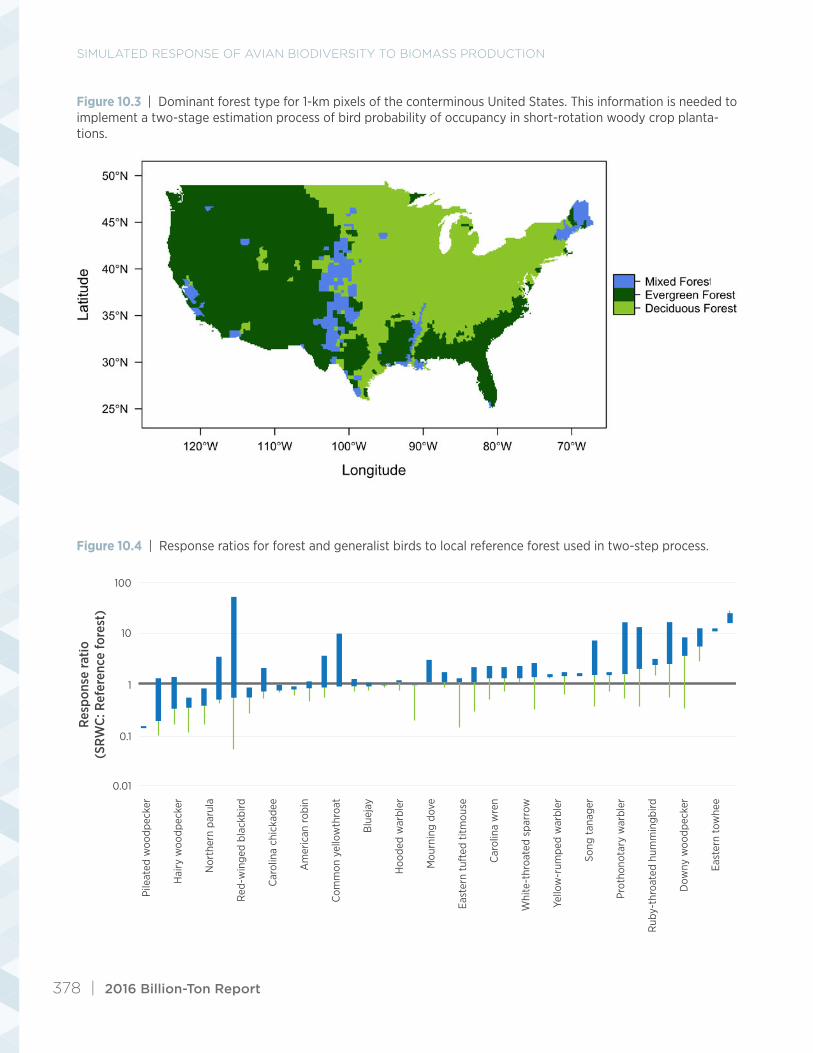
Projecting bird occupancy in future SRWC plan-tations on agricultural lands required a two-step process (fig. 10.2). We estimated the habitat value of the locally prevalent forest type (fig. 10.3) before ap-plying the forest-to-SRWC plantation response ratio (fig. 10.4). Note, this is simply an accounting trick

because many studies have compared bird densities in managed LULC to densities in forest, but none have compared densities in different managed LULC including one managed for biomass crops. In other words, transition of forest lands to SRWC was not simulated in the BC1 2040 scenario. We ob-tained SDM predictions of occupancy probabilities, P[s|x, Lj], by creating a transitional national LULC map, where the grid cells in the baseline LULC map with SWRCs under future scenarios were substituted by locally prevalent forest types. Next, we applied the conversion from equation 10.3 using the appro-priate response ratios reported for 40 birds found in forest or open woodland and edge habitat (Riffell et al. 2011).



Figure 10.3 | Dominant forest type for 1-km pixels of the conterminous United States. This information is needed to implement a two-stage estimation process of bird probability of occupancy in short-rotation woody crop planta-tions.

Figure 10.4 | Response ratios for forest and generalist birds to local reference forest used in two-step process.

100

10

1

0.1

0.01

Resp

onse

ratio

(SRW

C: R

efer

ence

fore

st)

Pile

ated

woo

dpec

ker

Nor

ther

n pa

rula

Hai

ry w

oodp

ecke

r

Red

-win

ged

blac

kbird

Car

olin

a ch

icka

dee

Am

eric

an ro

bin

Com

mon

yel

low

thro

at

Blu

ejay

Hoo

ded

war

bler

Mou

rnin

g do

ve

East

ern

tuft

ed t

itmou

se

Car

olin

a w

ren

Whi

te-t

hroa

ted

spar

row

Yello

w-r

umpe

d w

arbl

er

Prot

hono

tary

war

bler

Song

tan

ager

Rub

y-th

roat

ed h

umm

ingb

ird

Dow

ny w

oodp

ecke

r

East

ern

tow

hee


10.3.5.4 Perennial Grasses (Switchgrass and Miscanthus)

For switchgrass, we used estimated response ratios summarized by Robertson et al. (2012) based on data collected from Fletcher et al. (2011) for 12 grassland bird species (fig. 10.5). Comparisons allowing us to model transitions to switchgrass were available for three classes of agricultural LULC: (1) pasture/grass-land and hay; (2) row crops (as defined by Robertson et al. [2012]) including corn, cotton, and soybean; and (3) small grains, including barley, sorghum, rice,

oats, and wheat (fig. 10.2). To account for harvest management for switchgrass, we multiplied by an additional management response ratio, i.e., the ratio of bird density in switchgrass fields harvested in a certain way to its density in unharvested switchgrass (fig. 10.5). Bird densities were reported for switch-grass fields with strip harvest and total harvest (Best and Murray 2003). Thus, for switchgrass, we have comparable densities for bird species in three extant LULC classes (small grains, pasture, and row crops) and in switchgrass managed in each of two ways.

Figure 10.5 | Response ratios for grassland birds in total- and strip-harvested switchgrass (SWG).

50

5

0.5

0.05

0.005

Resp

onse

ratio

(Sw

itchg

rass

: Ref

eren

ce L

ULC

)

Hen

slow

’s s

parr

ow

Gra

ssho

pper

spa

rrow

Upl

and

sand

pipe

r

Nor

ther

n ha

rrie

r

Nor

ther

n bo

bwhi

te

Bob

olin

k

Sava

nnah

spa

rrow

Rin

g-ne

cked

phe

asan

t

Dic

kcis

sel

Fiel

d sp

arro

w

East

ern

mea

dow

lark

East

ern

king

bird

SWG: row crop

SWG strip: pasture/hay

SWG: small grain SWG: pasture/hay SWG strip: row crop SWG strip: small grain



olds. By overlaying the patch raster and the habitat SDM and removing habitat areas associated with small patches, we accounted for area sensitivities of birds. Therefore, CLU parcels that might otherwise have had a positive probability of occupancy (habitat value) were considered unoccupied if the total area of the patch and surrounding lands (including public lands), was too small to support the species. The “ras-ter” package in R was used to define habitat patches and to calculate patch sizes.

As a test case, we compared the estimated number of occupied grid cells for 2014 and the future map consistent with BC1 2040 for grassland birds with estimates of minimum area requirements >0 (appen-dix A, table 1; fig. 10.6).

For miscanthus, we adopted a ‘precautionary’ ap-proach. Published studies related to the suitability of miscanthus as a habitat are not yet available for birds in the United States (Vandever and Allen 2015). At this point, there is no evidence that miscanthus is used as nesting habitat for songbirds4 in the Midwest, and songbird densities in miscanthus were much lower than densities in surrounding grasslands.5 Therefore, we assumed that parcels that transitioned to miscanthus had zero habitat value.

10.3.6 Accounting for Minimum Area RequirementsA subset of species with specialized habitat needs require a minimum area of habitat to persist in habitat patches. Bio-EST can account for such area thresh-

Figure 10.6 | Minimum habitat area requirements for selected bird species

70

60

50

40

30

20

10

0

Min

imum

are

a re

quire

men

t (ha

)

56

46

16 15 12.4 10 105.5

25

0.54 0

Upl

and

sand

pipe

r

Bob

olin

k

Nor

ther

n ha

rrie

r

Nor

ther

n bo

bwhi

te

Hen

slow

’s s

parr

ow

Sava

nnah

spa

rrow

Gra

ssho

pper

spa

rrow

Rin

g-ne

cked

phe

asan

t

Dic

kcis

sel

Fiel

d sp

arro

w

East

ern

mea

dow

lark

East

ern

king

bird

4 Songbirds are in the order Passeriform (i.e., ‘perching birds’), which includes most grassland birds considered here. Non-passerine species considered here include the upland sandpiper and ring-necked pheasant.

5 R. L. Schooley, University of Illinois, email to H. Jager, June 23, 2016.


Figure 10.7 | Performance metrics for species distribution models for 52 bird species (each point) calculated for the test subset of data. Each point represents one species.

Kapp

a st

atis

tic

Species distribution model accuracy

0.0

0.80

0.40

0.20

0.60

1.20

1.00

0.70 0.75 0.80 0.85 0.90 0.95 1.00

Grassland Forest Generalist

10.3.7 Projecting Changes in RichnessThe methodology above (equations 10.2–10.3) allowed us to generate raster maps quantifying the likelihood of occurrence for each species. Richness maps result from aggregating predicted occurrences for three groups of species: a set of 12 predominantly grassland species and two sets of “forest” species for which we have data describing transitions to SRWC (see appendix A), referred to as forest specialists and generalists. For grid cells, we added the occupancy probabilities across the map to estimate the num-ber of occupied 1-km2 grid cells. For counties, we estimated the number of counties occupied in 2014 versus 2040 (BC1 2040), the change in the estimated number of occupied counties, and changes in rich-ness. Analyses are reported separately for the grass-land, forest specialist, and forest generalist species. Data were available to model LULC transitions to perennial grasses and energy sorghum (not SRWCs)

for birds in the grassland group. Data were also available to model LULC transitions to SRWCs and energy sorghum (but not perennial grasses) for birds in the forest specialist and generalist groups. We recognize that there is some subjectivity in how these sets are defined.

10.4 Results

10.4.1 Species Distribution ModelingOverall, the performance of SDMs was excellent. For the testing set, accuracy varied from 0.71 to 1.0 (all p-value <0.0001) across the 52 bird species modeled (fig. 10.7). Kappa statistics on the same set varied from 0.42 to 1.0 (all p-value <0.0001), with 79% of the kappa statistics (i.e., 41 out of 52 species) exceed-ing 0.6. Kappa values above 0.6 demonstrate substan-tial strength of agreement (Landis and Koch 1977).



10.4.2 Minimum Habitat AreaIn an exploratory analysis, we removed small patches of habitat below the minimum habitat threshold of each grassland species. Because the effects were ap-plied to future occupancy maps of both the reference 2014 case and BC1 2040 scenario, the resulting dif-ferences in range, measured in the number of counties occupied, were small and very similar for the 2014 and future landscapes (average 2.85% [SD = 0.68%] difference for 2014 map, 2.88% [SD = 0.62%] for BC1 2040 with strip harvest). Therefore, results pre-sented here do not consider minimum habitat area.

10.4.3 Projected Changes in Richness under BC1 2040 ScenarioOur simulations excluding miscanthus showed no change in projected occupancy from the 2014 to the

BC1 2040 landscape for most 1×1-km grid cells (>98% for both groups). However, in addition to lack of response to LULC change, this result is partly because we did not have information to simulate all possible transitions and partly because non-private lands were not permitted to change LULC. Decreases were projected in 0.13% of grid cells for grassland species, 1.4% for forest specialists, and 0.36% for generalists. Increases were projected in 1% of grid cells for grassland species, 0.07% for specialists, and 1.13% for generalists (fig 10.8).

Geographic patterns in grassland species reflect re-sponses to management of agricultural lands to BC1 2040 future switchgrass (strip harvest) and energy sorghum (fig. 10.9, top row). Patterns for forest Projected decreases appear to be concentrated in the middle of the country (fig. 10.9).

Figure 10.8 | Change in the estimated percentage of counties occupied by grassland bird species between the 2014 landscape and a future landscape consistent with the BC1 2040 scenario. Results are shown for two manage-ment regimes include strip harvest and total harvest of switchgrass (SWG).

Perc

ent c

hang

e in

occ

upie

d co

untie

s20

14 to

BC1

20

40

-5.0

1.0

0.0

-3.0

-4.0

-1.0

-2.0

5.0

4.0

3.0

2.0

Savan

nah sp

arrow

Henslow’s s

parrow

Northern harr

ier

Eastern m

eadowlar

k

Grassh

opper sparr

ow

Bobolink

Dickcis

sel

Eastern ki

ngbird

Upland sa

ndpiper

Northern bobwhite

Field sparr

ow

Ring-necked pheasa

nt

SWG strip harvest SWG total harvest


Figure 10.9 | Change in projected richness under the 2014 landscape (left column), a landscape consistent with the BC1 2040 future scenario (middle column) and differences (right column) for three groups of species. Rows display distributions for grassland, generalist, and forest specialist species. The range for differences in richness displayed by the legend row (below headers) is indicated below each map.

Current 2014 landscapeGroup/Legend

Grassland birds,(switchgrass

strip-harvested)(12 species)

Generalists(24 species)

Forest specialists(16 species)

Future BC1-2040 landscape Change in richness (# species)

0.40 to 9.60 species 0.40 to 10.21 species -4.10 to 3.02 species



For forest birds (specialist and generalist species), no change in richness was estimated for 99.2% of grid cells between the 2014 and the BC1 2040 LULC..

Increases occurred in <1% of the grid cells for both forest generalists and specialists. Likewise, decreases occurred in <1% for both types. (fig. 10.10).



Figure 10.10 | Change in the modeled percentage of counties occupied by species designated for purposes of this analysis as a) forest specialist and b) generalist bird species between the 2014 landscape and a future landscape consistent with the BC1 2040 scenario.

% c

hang

e in

occ

upie

d co

untie

s 2

014

to B

C1 2

040

-5.0

1.0

-1.0

-3.0

5.0

3.0

Nor

ther

n pa

rula

Gre

at-c

rest

ed fl

ycat

cher

Pile

ated

woo

dpec

ker

Hai

ry w

oodp

ecke

r

Red

-bel

lied

woo

dpec

ker

Car

olin

a ch

icka

dee

Woo

d th

rush

Nor

ther

n ca

rdin

al

Blu

e-gr

ay g

natc

atch

er

Prot

hono

tary

war

bler

Red

-eye

d vi

reo

Kent

ucky

war

bler

Hoo

ded

war

bler

Aca

dian

flyc

atch

er

Sum

mer

tan

ager

War

blin

g vi

reo

% c

hang

e in

occ

upie

d co

untie

s 2

014

to B

C1 2

040

-5.0

1.0

-1.0

-3.0

5.0

3.0

Red

-win

ged

blac

kbird

Bro

wn-

head

ed c

owbi

rd

Mou

rnin

g do

ve

Whi

te-e

yed

vire

o

Yello

w-b

illed

cuc

koo

Yello

w-r

umpe

d w

arbl

er

East

ern

blue

bird

Dow

ny w

oodp

ecke

r

Red

-hea

ded

woo

dpec

ker

Bro

wn

thra

sher

East

ern

tuft

ed t

itmou

se

Rub

y-th

roat

ed h

umm

ingb

ird

Am

eric

an ro

bin

Car

olin

a w

ren

Blu

e ja

y

Com

mon

gra

ckle

Indi

go b

untin

g

Whi

te-t

hroa

ted

spar

row

Am

eric

an g

oldfi

nch

Yello

w-b

reas

ted

chat

East

ern

tow

hee

Com

mon

yel

low

thro

at

Song

spa

rrow

Orc

hard

orio

le


To understand the LULC changes driving these results, we summarized LULC changes that would result in changes of more than 80% in richness at the grid-cell scale, all of which were planted in switch-grass in the BC1 2040 landscape. Positive changes in grassland bird richness were dominated by grid cells that were planted in cotton or corn in 2014 (1,138 grid cells), whereas negative changes were domi-nated by grid cells planted in pasture or hay in 2014 (14,777 grid cells). Grid cells with positive chang-es in generalist bird species were planted in corn (19 grid cells) or wheat (11 grid cells) in the 2014 landscape and non-coppice wood (poplar) in the BC1 2040 landscape. Grid cells that decreased in richness were in coppice wood (willow) in the BC1 2040 landscape and pasture (70 grid cells) or soybeans (20 grid cells) in the 2014 landscape. Grid cells associ-ated with negative changes in the number of forest bird specialists were predominantly in coppice wood (willow) in the BC1 2040 landscape and in soybeans (3,057 cells) or corn (144 cells) in 2014.

10.5 DiscussionResults presented here for grassland and woodland/forest birds in the BC1 2040 scenario are consistent with our expectations about the potential costs and/or benefits of growing dedicated bioenergy crops. Among grassland birds, projections showed the po-tential for increases in range for ring-necked pheasant and field sparrow, and decreases (or no change) for others. It is important to note that our assumptions about miscanthus were precautionary (we assumed zero habitat value for this crop, which represented 77,821 km2 in the BC1 2040 landscape). Interesting-ly, strip harvest did not consistently increase occu-pancy across grassland species compared with total harvest. It should be noted that grassland-obligate species are better served by patches of habitat with high area-to-perimeter ratios, i.e., blocks, not strips (Helzer and Jelinski 1999; Roth et al. 2005).

Further analysis to understand how different taxa responded could help to explain the risk or benefits to

species with different life histories and habitat needs. The analysis presented here can also be extended to represent other wildlife taxa once enough compari-sons of wildlife performance (e.g., density, reproduc-tive success) in multiple food crop and biomass crop habitats have been made. For example, studies have quantified the benefits of energy crops as a habitat for pollinators (Meehan et al. 2012; Bennett et al. 2014; Bennett and Isaacs 2014) and for other beneficial insects, for example, those that provide pest-control services (Werling et al. 2011). In comparison to birds, few studies have focused on quantifying the habitat value of biomass crops for other taxa (e.g., mammals, amphibians, and reptiles).

Our analysis involved some simplifying assumptions to allow for a national-scale assessment. It uses an implicit “equilibrium” assumption. In other words, we compare a recent landscape with one potential future landscape, but not with transient influences of the crop transition on occupancy, which could incur higher, but possibly temporary, impacts. The tim-ing of management changes might help to alleviate potential stresses caused by change. Birds are mobile taxa that could be more resilient to changes in land management than other taxa, except during mating, nesting, and incubation.

Finally, we join other ecologists by offering the sug-gestion that benefits to birds (and other wildlife) can be attained by implementing wildlife-friendly practic-es (Meehan, Hulbert, and Gratton 2010; Robertson et al. 2012; Ridley et al. 2013). Birds tend to be at their most vulnerable to disturbance by management activ-ities during nesting. Impacts to nests can be avoid-ed by timing farm operations prior to the summer nesting season and between harvest and the summer nesting season. Timing harvest to occur outside of the nesting season is more feasible for grasses grown for biomass than for hay and other crops that quickly lose their quality as forage for animals if harvested in the fall. Furthermore, potential for harvest after winter can be explored to provide resident birds with cover and forage during winter. In addition, using a



flushing bar and raising the height of mowing equip-ment can help to avoid nests and animals during farm operations; and, simply harvesting from the inside out, instead of trapping wildlife in the center of a field, can be beneficial. These, and other best-man-agement practices can help to manage bioenergy crops with an eye toward protecting biodiversity (McGuire and Rupp 2013; Brooke et al. 2009).

10.6 Future DirectionsFuture research can address ways to design bio-mass-production methods that benefit biodiversity, as well as producing feedstocks for bioenergy or other uses:

• Research is required to increase the feasibility of production systems that employ more diverse communities of plants as feedstocks, including forbs and other plants typically found in native prairie. Such plant communities have been found to support more diverse communities of insects and possibly other taxa. In conjunction with research on diverse feedstock production, research is needed to understand barriers to the conversion of complex cellulosic feedstock streams.

• This assessment relied on field comparisons of wildlife in other crops or LULC classes and biomass-producing lands. These data are needed to quantify the responses to bioenergy crops by

other taxa. In particular, information about po-tential habitat value of miscanthus and eucalyp-tus is lacking. These non-native species may or may not provide similar habitat to pre-existing native vegetation.

• Research is needed to understand logistic and economic barriers that could prevent farmers from adopting practices that benefit wildlife. Some of these barriers might be overcome by developing innovative technologies (smart trac-tor systems) and new wildlife-friendly practices.

• The relative effects of pesticide use for bioener-gy feedstocks and for other managed lands, as well as trade-offs between pesticide use and oth-er potentially beneficial practices (e.g., tillage), have not been studied and quantified or related to wildlife performance.

• Benefits of seed-producing crops to wildlife are well known (Guthery 1997). However, the wild-life and production co-benefits of integrating production of biodiesel crops, such as soybeans and canola, with cellulosic feedstock production have not been explored.

• Future research can help to identify geographic hotspots where attention to wildlife-friendly practices is needed. In addition, trait-based guidance can be developed to guide farmers and SRWC growers toward practices that protect and support local wildlife of conservation concern.


10.7 References Ando, A. 1998. “Species Distributions, Land Values, and Efficient Conservation.” Science 279 (5359): 2126–8.

doi:10.1126/science.279.5359.2126.

Askins, R. A., F. Chavez-Ramirez, B. C. Dale, C. A. Haas, J. R. Herkert, F. L. Knopf, and P. D. Vickery. 2007. “Conservation of Grassland Birds in North America: Understanding Ecological Processes in Differ-ent Regions. Report of the AOU Committee on Conservation.” Ornithological Monographs 64: 1–46. doi:10.2307/40166905.

Barbet-Massin, Morgane, Frederic Jiguet, Cecile Helene Albert, and Wilfried Thuiller. 2012. “Selecting pseu-do-absences for species distribution models: how, where and how many?” Methods in Ecology and Evolu-tion 3 (2): 327–38. doi:10.1111/j.2041-210X.2011.00172.x.

Batt, S. 2009. “Human attitudes towards animals in relation to species similarity to humans: a multivariate ap-proach.” Bioscience Horizons 2 (2): 180–190. doi:10.1093/biohorizons/hzp021:11.

Bennett, A. B., and R. Isaacs. 2014. “Landscape composition influences pollinators and pollination services in perennial biofuel plantings.” Agriculture Ecosystems & Environment 193 (1): 1–8. doi:10.1016/j.agee.2014.04.016.

Bennett, A. B., T. D. Meehan, C. Gratton, and R. Isaacs. 2014. “Modeling Pollinator Community Response to Contrasting Bioenergy Scenarios.” Plos One 9 (11). doi:10.1371/journal.pone.0110676.

Best, L. B., and L. D. Murray. 2003. “Bird responses to harvesting switchgrass fields for biomass.” In Transac-tions of the Sixty-Ninth North American Wildlife and Natural Resources Conference, edited by J. Rahm, 224–35.

Blank, P. J., D. W. Sample, C. L. Williams, and M. G. Turner. 2014. “Bird communitites and biomass yields in potential bioenergy grasslands.” PLOS ONE 9 (10): 1–10. doi:10.1371/journal.pone.0109989.

Booth, T. H., H. A. Nix, J. R. Busby, and M. F. Hutchinson. 2014. “Bioclim: The first species distribution model-ling package, its early applications and relevance to most current MaxEnt studies.” Diversity and Distribu-tions 20 (1): 1–9. doi:10.1111/ddi.12144.

Brooke, R, G. Fogel, A. Glaser, E. Griffin, and K. Johnson. 2009. Corn Ethanol and Wildlife. Washington, DC: National Wildlife Federation. https://www.nwf.org/pdf/Wildlife/01-13-10-Corn-Ethanol-Wildlife.pdf.

Cook, J. H., J. Beyea, and K. H. Keeler. 1991a. “Biofuels - Answer to global warming or growing threat to bio-diversity?” In Forestry and Environment – Engineering Solutions, Proceedings of the American Society of Agricultural Engineers, June 5–6, edited by B. J. Stokes and C. L. Rawlins, 21–31.

Cook, J. H., J. Beyea, and K. H. Keeler. 1991b. “Potential Impacts of Biomass Production in the United States on Biological Diversity.” Annual Review of Energy and the Environment 16: 401–31. doi:10.1146/an-nurev.eg.16.110191.002153.

Dale, V. H., E. S. Parish, and K. L. Kline. 2015. “Risks to global biodiversity from fossil-fuel production exceed those from biofuel production.” Biofuels Bioproducts & Biorefining 9 (2): 177–89. doi:10.1002/bbb.1528.

http://science.sciencemag.org/content/279/5359/2126

https://www.jstor.org/stable/40166905?seq=1#page_scan_tab_contents

https://www.researchgate.net/publication/247577631_Human_attitudes_towards_animals_in_relation_to_species_similarity_to_humans_A_multivariate_approach

https://www.researchgate.net/publication/247577631_Human_attitudes_towards_animals_in_relation_to_species_similarity_to_humans_A_multivariate_approach

http://www.sciencedirect.com/science/article/pii/S0167880914002229


http://journals.plos.org/plosone/article?id=10.1371/journal.pone.0110676


http://onlinelibrary.wiley.com/doi/10.1111/ddi.12144/abstract

https://www.nwf.org/pdf/Wildlife/01-13-10-Corn-Ethanol-Wildlife.pdf

http://www.annualreviews.org/doi/abs/10.1146/annurev.eg.16.110191.002153

http://www.annualreviews.org/doi/abs/10.1146/annurev.eg.16.110191.002153

http://onlinelibrary.wiley.com/doi/10.1002/bbb.1528/abstract



Elith, J., J. R. Leathwick, and T. Hastie. 2008. “A working guide to boosted regression trees.” Journal of Animal Ecology 77 (4): 802–13. doi:10.1111/j.1365-2656.2008.01390.x.

Evans, S. G., L. C. Kelley, and M. D. Potts. 2014. “The potential impact of second-generation biofuel land-scapes on at-risk species in the US.” Global Change Biology Bioenergy 7 (2): 337–48. doi:10.1111/gcbb.12131.

Fenoglio, S., T. Bo, M. Cucco, L. Mercalli, and G. Malacarne. 2010. “Effects of global climate change on fresh-water biota: A review with special emphasis on the Italian situation.” Italian Journal of Zoology 77 (4): 374–83. doi:10.1080/11250000903176497.

Fletcher, R. J., B. A. Robertson, J. Evans, P. J. Doran, J. R. R. Alavalapati, and D. W. Schemske. 2011. “Biodi-versity conservation in the era of biofuels: risks and opportunities.” Frontiers in Ecology and the Envi-ronment 9 (3): 161–8. doi:10.1890/090091.

Guillera-Arroita, Gurutzeta, Jose J. Lahoz-Monfort, Jane Elith, Ascelin Gordon, Heini Kujala, Pia E. Lentini, Michael A. McCarthy, Reid Tingley, and Brendan A. Wintle. 2015. “Is my species distribution model fit for purpose? Matching data and models to applications.” Global Ecology and Biogeography 24 (3): 276–92. doi:10.1111/geb.12268.

Guthery, F. S. 1997. “A philosophy of habitat management for northern bobwhites.” Journal of Wildlife Man-agement 61 (2): 291–301. doi:10.2307/3802584.

Helzer, C. J., and D. E. Jelinski. 1999. “The relative importance of patch area and perimeter-area ratio to grass-land breeding birds.” Ecological Applications 9 (4): 1448–58. doi:10.1890/1051-0761(1999)009[1448:TRIOPA]2.0.CO;2.

Herkert, J. R. 1994. “The effects of habitat fragmentation on Midwestern grassland bird communities.” Ecologi-cal Applications 4 (3): 461–71. doi:10.2307/1941950.

Herkert, J. R., S. A. Simpson, R. L. Westermeier, T. L. Esker, and J. W. Walk. 1999. “Response of northern har-riers and short-eared owls to grassland management in Illinois.” Journal of Wildlife Management 63 (2): 517–23. doi:10.2307/3802637.

Hertzog, L. R., A. Besnard, and P. Jay-Robert. 2014. “Field validation shows bias-corrected pseudo-absence selection is the best method for predictive species-distribution modelling.” Diversity and Distributions 20 (12):1403–13. doi:10.1111/ddi.12249.

Hijmans, R. J., and C. H. Graham. 2006. “The ability of climate envelope models to predict the effect of cli-mate change on species distributions.” Global Change Biology 12 (12): 2272–81. doi:10.1111/j.1365-2486.2006.01256.x.

Johnson, D. H., and L. D. Igl. 2001. “Area requirements of grassland birds: A regional perspective.” Auk 118 (1): 24–34. doi:10.1642/0004-8038(2001)118[0024:arogba]2.0.co;2.

Kobal, S. N., N. F. Payne, and D. R. Ludwig. 1999. “Habitat/area relationships, abundance, and composition of bird communities in 3 grassland types.” Transactions of the Illinois State Academy of Science 92 (1–2): 109–31. http://ilacadofsci.com/wp-content/uploads/2013/08/092-12MS9808-print.pdf.

Kuhn, M. 2008. “Building Predictive Models in R Using the caret Package.” Journal of Statistical Software 28 (5): 1–26. doi:10.18637/jss.v028.i05.

https://www.ncbi.nlm.nih.gov/pubmed/18397250

http://onlinelibrary.wiley.com/doi/10.1111/gcbb.12131/abstract

http://onlinelibrary.wiley.com/doi/10.1111/gcbb.12131/abstract

http://www.tandfonline.com/doi/abs/10.1080/11250000903176497

http://onlinelibrary.wiley.com/doi/10.1890/090091/abstract

http://onlinelibrary.wiley.com/doi/10.1111/geb.12268/abstract


http://onlinelibrary.wiley.com/doi/10.1890/1051-0761(1999)009%5B1448:TRIOPA%5D2.0.CO;2/abstract

http://onlinelibrary.wiley.com/doi/10.1890/1051-0761(1999)009%5B1448:TRIOPA%5D2.0.CO;2/abstract

https://www.jstor.org/stable/3802637




https://www.researchgate.net/publication/279935344_Area_requirements_of_grassland_birds_A_regional_perspective

http://ilacadofsci.com/wp-content/uploads/2013/08/092-12MS9808-print.pdf

https://www.jstatsoft.org/article/view/v028i05


Landis, J. R., and G. G. Koch. 1977. “The measurement of observer agreement for categorical data.” Biometrics 33 (1): 159–74. doi:10.2307/2529310.

Lawler, J. J., D. J. Lewis, E. J. Nelson, A. J. Plantinga, S. Polasky, J. C. Withey, D. P. Helmers, S. Martinuzzi, D. Pennington, and V. C. Radeloff. 2014. “Projected land-use change impacts on ecosystem services in the United States.” Proceedings of the National Academy of Sciences 111 (20): 7492–7. doi:10.1073/pnas.1405557111.

Matthews, Stephen N., Louis R. Iverson, Anantha M. Prasad, and Matthew P. Peters. 2011. “Changes in poten-tial habitat of 147 North American breeding bird species in response to redistribution of trees and climate following predicted climate change.” Ecography 34 (6): 933–45. doi:10.1111/j.1600-0587.2011.06803.x.

McGuire, B., and S. Rupp. 2013. Perennial herbaceous biomass production and harvest in the prairie pothole region of the Northern Great Plains: Best management guidelines to achieve sustainability of wildlife resources. Washington, DC: National Wildlife Federation. http://www.nwf.org/~/media/PDFs/Wildlife/BiomassBMGPPR.pdf.

Meehan, T. D., A. H. Hurlbert, and C. Gratton. 2010. “Bird communities in future bioenergy landscapes of the Upper Midwest.” Proceedings of the National Academy of Sciences of the United States of America 107 (43): 18533–8. doi:10.1073/pnas.1008475107.

Meehan, T. D., B. P. Werling, D. A. Landis, and C. Gratton. 2012. “Pest-Suppression Potential of Midwestern Landscapes under Contrasting Bioenergy Scenarios.” Plos One 7 (7). doi:10.1371/journal.pone.0041728.

Pe’er, G., M. A. Tsianou, K. W. Franz, Y. G. Matsinos, A. D. Mazaris, D. Storch, L. Kopsova, J. Verboom, M. Baguette, V. M. Stevens, and K. Henle. 2014. “Toward better application of minimum area requirements in conservation planning.” Biological Conservation 170: 92–102. doi:10.1016/j.biocon.2013.12.011.

Phillips, S. J., M. Dudik, J. Elith, C. H. Graham, A. Lehmann, J. R. Leathwick, and S. Ferrier. 2009. “Sample selection bias and presence-only distribution models: implications for background and pseudo-absence data.” Ecological Applications 19 (1): 181–97. doi:10.1890/07-2153.1.

Rashford, B. S., J. A. Walker, and C. T. Bastian. 2011. “Economics of Grassland Conversion to Cropland in the Prairie Pothole Region.” Conservation Biology 25 (2): 276–84. doi:10.1111/j.1523-1739.2010.01618.x.

Ridley, C. E., H. I. Jager, R. A. Efroymson, C. Kwit, D. A. Landis, Z. H. Leggett, D. A. Miller, and C. M. Clark. 2013. “Debate: Can bioenergy be produced in a sustainable manner that protects biodiversity and avoids the risk of invaders?” Ecological Society of America Bulletin 94 (3): 277–90. doi:10.1890/0012-9623-94.3.277.

Riffell, S., J. Verschuyl, D. Miller, and T. B. Wigley. 2011. “Biofuel harvests, coarse woody debris, and bio-diversity – A meta-analysis.” Forest Ecology and Management 261 (4): 878–87. doi:10.1016/j.fore-co.2010.12.021.

Robbins, C. S., D. K. Dawson, and B. A. Dowell. 1989. “Habitat area requirements of breeding forest birds of the Middle Atlantic states.” Wildlife Monographs (103): 1–34. http://www.jstor.org/stable/383069.

Robertson, B. A., R. A. Rice, T. S. Sillett, C. A. Ribic, B. A. Babcock, D. A. Landis, J. R. Herkert, R. J. Fletcher, J. J. Fontaine, P. J. Doran, and D. W. Schemske. 2012. “Are Agrofuels a Conservation Threat or Opportunity for Grassland Birds in the United States?” The Condor 114 (4): 679–88. doi:10.1525/cond.2012.110136.


http://www.pnas.org/content/111/20/7492.abstract


http://onlinelibrary.wiley.com/doi/10.1111/j.1600-0587.2011.06803.x/abstract

http://www.nwf.org/~/media/PDFs/Wildlife/BiomassBMGPPR.pdf

http://www.nwf.org/~/media/PDFs/Wildlife/BiomassBMGPPR.pdf




http://onlinelibrary.wiley.com/doi/10.1890/07-2153.1/full

http://onlinelibrary.wiley.com/doi/10.1111/j.1523-1739.2010.01618.x/full

http://onlinelibrary.wiley.com/doi/10.1890/0012-9623-94.3.277/abstract

http://onlinelibrary.wiley.com/doi/10.1890/0012-9623-94.3.277/abstract



http://www.jstor.org/stable/383069

http://www.jstor.org/stable/10.1525/cond.2012.110136?seq=1#page_scan_tab_contents

http://www.jstor.org/stable/10.1525/cond.2012.110136?seq=1#page_scan_tab_contents



Rondinini, C., K. A. Wilson, L. Boitani, H. Grantham, and H. P. Possingham. 2006. “Tradeoffs of different types of species occurrence data for use in systematic conservation planning.” Ecology Letters 9 (10): 1136–45. doi:10.1111/j.1461-0248.2006.00970.x.

Roth, A. M., D. W. Sample, C. A. Ribic, L. Paine, D. J. Undersander, and G. A. Bartelt. 2005. “Grassland bird response to harvesting switchgrass as a biomass energy crop.” Biomass & Bioenergy 28 (5): 490–8. doi:10.1016/j.biombioe.2004.11.001.

Royle, J. A., and J. D. Nichols. 2003. “Estimating abundance from repeated presence-absence data or point counts.” Ecology 84 (3): 777–90. doi:10.1890/0012-9658(2003)084[0777:eafrpa]2.0.co;2.

Samson, F. B., F. L. Knopf, and W. R. Ostlie. 2004. “Great Plains ecosystems: past, present, and future.” Wild-life Society Bulletin 32 (1): 6–15. doi:10.2193/0091-7648(2004)32[6:gpeppa]2.0.co;2.

Stoms, D. M., F. W. Davis, M. W. Jenner, T. M. Nogeire, and S. R. Kaffka. 2012. “Modeling wildlife and other trade-offs with biofuel crop production.” Global Change Biology Bioenergy 4 (3): 330–41. doi:10.1111/j.1757-1707.2011.01130.x.

Tavernia, B. G., M. D. Nelson, M. E. Goerndt, B. F. Walters, and C. Toney. 2013. “Changes in forest habitat classes under alternative climate and land-use change scenarios in the northeast and midwest, USA.” Mathematical and Computational Forestry and Natural-Resource Sciences 5 (2): 135–50. http://www.fs.fed.us/nrs/pubs/jrnl/2013/nrs_2013_Tavernia_002.pdf?.

Terhune, T. M., D. C. Sisson, W. E. Palmer, B. C. Faircloth, H. L. Stribling, and J. P. Carroll. 2010. “Transloca-tion to a fragmented landscape: survival, movement, and site fidelity of Northern Bobwhites.” Ecological Applications 20 (4): 1040–52. doi:10.1890/09-1106.1.

Tirpak, J. M., D. T. Jones-Farrand, III F. R. Thompson, D. J. Twedt, and W.B. Uihlein III. 2008. Multiscale hab-itat suitability index models for priority landbirds in the Central Hardwoods and West Gulf Coastal Plain / Ouachitas bird conservation regions. Delaware, OH: U.S. Department of Agriculture, Forest Service, Northern Research Station. http://www.nrs.fs.fed.us/pubs/gtr/gtr_nrs49.pdf?.

USDA. 1999. Northern Bobwhite (Colinus virginianus). Madison, MS: U.S. Department of Agriculture, Wildlife Habitat Management Institute, Natural Resources Conservation Service. http://www.chenangoswcd.org/chenango/linked/bobwhite.pdf.

USDA. 2014. Common Land Unit Database. Washington, D.C.: US Department of Agriculture, Farm Service Agency, pp.

USFWS (U.S. Fish and Wildlife Service). 2008. Birds of Conservation Concern 2008. Arlington, Virginia: U. S. Department of the Interior, Fish and Wildlife Service, Division of Migratory Bird Management. https://www.fws.gov/migratorybirds/pdf/grants/BirdsofConservationConcern2008.pdf.

USGS. 2013. Biodiversity Information Serving Our Nation Database. Washington, DC.: US Geological Survey, pp. https://bison.usgs.gov/#home

Vance, M. D., L. Fahrig, and C. H. Flather. 2002. “Relationship between minimum habitat requirements and an-nual reproductive rates in forest breeding birds.” Ecological Society of America Annual Meeting Abstracts 87: 288–9.


https://pubs.er.usgs.gov/publication/70029266

http://onlinelibrary.wiley.com/doi/10.1890/0012-9658(2003)084%5b0777:EAFRPA%5d2.0.CO;2/abstract

http://onlinelibrary.wiley.com/doi/10.2193/0091-7648(2004)32%5B6:GPEPPA%5D2.0.CO;2/abstract



http://www.fs.fed.us/nrs/pubs/jrnl/2013/nrs_2013_Tavernia_002.pdf?

http://www.fs.fed.us/nrs/pubs/jrnl/2013/nrs_2013_Tavernia_002.pdf?


http://www.nrs.fs.fed.us/pubs/gtr/gtr_nrs49.pdf?

http://www.chenangoswcd.org/chenango/linked/bobwhite.pdf

http://www.chenangoswcd.org/chenango/linked/bobwhite.pdf

https://www.fws.gov/migratorybirds/pdf/grants/BirdsofConservationConcern2008.pdf

https://bison.usgs.gov/#home


Vandever, M. W., and A. W. Allen. 2015. Management of Conservation Reserve Program Grasslands to Meet Wildlife Habitat Objectives. Reston, VA: U.S. Department of the Interior, U.S. Geological Survey. https://pubs.usgs.gov/sir/2015/5070/pdf/sir2015-5070.pdf.

Vickery, P. D., M. L. Hunter, and S. M. Melvin. 1994. “Effects of habitat area on the distribution of grassland birds in Maine.” Conservation Biology 8 (4): 1087–97. doi:10.1046/j.1523-1739.1994.08041087.x.

Vickery, P. D., P. L. Tubaro, J. M. C. da Silva, B. G. Peterjohn, J. R. Herkert, and R. B. Cavalcanti. 1999. “Conservation of grassland birds in the Western Hemisphere.”. In Ecology and Conservation of Grass-land Birds of the Western Hemisphere, edited by P. D. Vickery and J. R. Herkert. Lawrence, KS: Cooper Ornitholigical Society. https://sora.unm.edu/sites/default/files/journals/sab/sab_019.pdf.

Werling, B. P., T. D. Meehan, C. Gratton, and D. A. Landis. 2011. “Influence of habitat and landscape peren-niality on insect natural enemies in three candidate biofuel crops.” Biological Control 59 (2): 304–12. doi:10.1016/j.biocontrol.2011.06.014.

Withey, J. C., J. J. Lawler, S. Polasky, A. J. Plantinga, E. J. Nelson, P. Kareiva, C. B. Wilsey, C. A. Schloss, T. M. Nogeire, A. Ruesch, J. Ramos, and W. Reid. 2012. “Maximising return on conservation investment in the conterminous USA.” Ecology Letters 15: 1249–56. doi:10.1111/j.1461-0248.2012.01847.x.

https://pubs.usgs.gov/sir/2015/5070/pdf/sir2015-5070.pdf


https://sora.unm.edu/sites/default/files/journals/sab/sab_019.pdf





Appendix 10-A Table 10A.1. | Bird species included in our analysis. References for minimum area requirements of forest, shru-bland, or generalist birds include: Galli, Leck, and Forman 1976; Robbins, Dawson, and Dowell 1989; Pe’er et al. 2014; Vance, Fahrig, and Flather 2002; and Tirpak et al. 2008. References for minimum area requirements of grassland birds include: Herkert 1994; Herkert et al. 1999; Helzer and Jelinski 1999; Kobal, Payne, and Ludwig 1999; Johnson and Igl 2001; Terhune et al. 2010; USDA 1999; and Vickery, Hunter, and Melvin 1994. We defined minimum area as the area associated with a 50% probability of occupancy.

Common name

Scientific name

Primary habitat

Minimum area

required (km2)

Species considered to prefer

patch edges or patch interiors

Neotropical/ North

American/ Resident

Reference ecosystems

Forest Corn Prairie Small grain

BobolinkDolichonyx oryzivorus

Mixed grass-land, obligate

46 InteriorNorth

American• • • •

DickcisselSpiza

AmericanaMid-tallgrass 0.54 Interior Neotropical • • • •

Eastern kingbird

Tyrannus tyrannus

Open savannah

0Interior ground- nesting

Neotropical • • • •

Eastern meadowlark

Sturnella magna

Grassland obligate

5 Edge Neotropical • • • •

Field sparrowSpizella pusilla

Generalist 2 Generalist Neotropical • • • •

Grasshopper sparrow

Ammodramus savannarum

Shortgrass, obligate

10 InteriorNorth


Henslow’s sparrow

Ammodramus henslowii

Tallgrass, obligate

12.4Early succes-sion, ground

nesterNeotropical • • • •

Northern bobwhite

Colinus virginianus

Midgrass 16Early

successionNeotropical • • • •

Northern harrier

Circus cyaneus

Grassland 15 OpenNorth


Ring-necked pheasant

Phasianus colchicus

Tallgrass 5.5* Edge Resident • • • •

Savannah sparrow

Passerculus sandwichensis

Grassland, obligate;

open fields10 Interior

North American

• • • •

Upland sandpiper

Bartramia longicauda

Shortgrass 56 Interior Neotropical • • • •

*Considered area-independent, as are species with zero values listed.


Common name

Scientific name

Primary habitat

Minimum area

required (km2)



Neotropical/ North

American/ Resident



Acadian flycatcher

Empidonax virescens

Forest 15 Interior Neotropical •

American goldfinch

Spinus tristisGrassland,

open/riparian woodland

0 EdgeNorth Amer-ican migrant

•

American robin

Turdus migratorius

Generalist, woodland/ farmland

0.2*Open,

generalistNorth Amer-ican migrant

•

Blue jayCyanocitta

cristataForest 0.8

Open, generalist

Resident/North Amer-ican migrant

•

Blue-gray gnatcatcher

Polioptila caerulea


Brown thrasher

Toxostoma rufum

Forest 0*Early

successionalResident •

Carolina chickadee

Poecile carolinensis

Forest 0* (cavity nester) Resident •

Carolina wrenThryothorus ludovicianus

Forest 2* Generalist Resident •

Common grackle

Quiscalus quiscula

Forest 0.2* Edge Neotropical •

Downy woodpecker

Picoides pubescens

Forest 1.2Generalist,

(cavity nester)Resident •

Eastern towhee

Pipilo eryth-rophthal-mus

Forest 3*Generalist/

early succes-sional forest

Resident •

Eastern tufted titmouse

Baeolophus bicolor

Deciduous forest

2Edge/for-

est-shrublandNeotropical •

Great-crested flycatcher

Myiarchus crinitus

Forest 0.3*Interior

(cavity nester)Neotropical •

Hairy woodpecker

Picoides villosus

Forest 24Interior


Hooded warbler

Setophaga citrina

Forest 20Interior, but uses gaps, understory

Neotropical •

Indigo bunting

Passerina cyanea

Forest 10*Generalist,

edge, shrubsNeotropical •




Common name

Scientific name

Primary habitat

Minimum area

required (km2)



Neotropical/ North

American/ Resident



Kentucky warbler

Geothlypis formosa


Northern cardinal

Cardinalis cardinalis


Northern parula

Setophaga americana

Forest 520Woodland, shrubland

Resident •

Orchard orioleIcterus spurius

Deciduous forest

0Open forest,

edgeResident •

Pileated woodpecker

Dryocopus pileatus

Forest 165

Interior, (cavity nester),

forages in low foliage

Neotropical •

Prothonotary warbler

Protonotaria citrea

Forest 30Interior,


Red-bellied woodpecker

Melanerpes carolinus

Forest 7.5Interior,

(cavity nester)Neotropical •

Red-eyed vireo

Vireo olivaceus

Forest 2.5 Interior Resident •

Red-headed woodpecker

Melaner-pes eryth-

ro-cephalusForest 0 Generalist Neotropical •

Ruby-throated

hummingbird

Archilochus colubris

Forest, coniferous

0 Generalist Neotropical •

Summer tanager

Piranga rubraForest,

deciduous and mixed

40 Streams Neotropical •

Warbling vireo

Vireo gilvusForest,

deciduous and mixed

0Shrubby

understory in gaps

Neotropical •

White-eyed vireo

Vireo griseusForest,

deciduous5.9

Generalist, shrub, pas-

ture, (ground nester)

North American

•

White-throated sparrow

Zonotrichia albicollis

Forest 0Generalist,

(ground nester)

Neotropical •



Common name

Scientific name

Primary habitat

Minimum area

required (km2)



Neotropical/ North

American/ Resident



Wood thrushHylocichla mustelina


Yellow-billed cuckoo

Coccyzus americanus

Forest generalist

24Shrubs, cup

nesterNeotropical •

Yellow-breasted chat

Icteria virensForest,

coniferous, shrubland

0 (forest), 2.3 (shrub-

land)

Shrubs, cup nester

Neotropical •

Yellow-rumped warbler

Setophaga coronata

Generalist, coniferous

forest0 Edge

North American

•

Brown-headed cowbird

Molothrus ater

Grassland 0 Edge Neotropical • • •

Common yellowthroat

Geothlypis trichas

Forest 0Early

successionNeotropical • • •

Eastern bluebird

Sialia sialis Forest edge 0 Edge Neotropical • • •

Mourning dove

Zenaida macroura

Open woodland, grassland

4 EdgeResident/

North American

• • •

Red-winged blackbird

Agelaius phoeniceus

Grassland, wetland

24 Generalist Resident • • •

Song sparrowMelospiza melodia

Early succession

24* EdgeNorth

American• • •


This page was intentionally left blank.

10 simulated response of avian biodiversity to biomass ... · simulated response of avian...

Documents