10-year spatial and temporal trends of pm concentrations...

Atmos. Chem. Phys., 14, 6301–6314, 2014www.atmos-chem-phys.net/14/6301/2014/doi:10.5194/acp-14-6301-2014© Author(s) 2014. CC Attribution 3.0 License.

10-year spatial and temporal trends of PM2.5 concentrations in thesoutheastern US estimated using high-resolution satellite data

X. Hu1, L. A. Waller 2, A. Lyapustin3, Y. Wang3,4, and Y. Liu1

1Department of Environmental Health, Rollins School of Public Health, Emory University, Atlanta, GA 30322, USA2Department of Biostatistics & Bioinformatics, Rollins School of Public Health, Emory University, Atlanta, GA 30322, USA3NASA Goddard Space Flight Center, Greenbelt, MD, USA4University of Maryland Baltimore County, Baltimore, MD, USA

Correspondence to:Y. Liu ([email protected])

Received: 13 August 2013 – Published in Atmos. Chem. Phys. Discuss.: 7 October 2013Revised: 12 May 2014 – Accepted: 13 May 2014 – Published: 25 June 2014

Abstract. Long-term PM2.5 exposure has been associatedwith various adverse health outcomes. However, most groundmonitors are located in urban areas, leading to a potentiallybiased representation of true regional PM2.5 levels. To facili-tate epidemiological studies, accurate estimates of the spa-tiotemporally continuous distribution of PM2.5 concentra-tions are important. Satellite-retrieved aerosol optical depth(AOD) has been increasingly used for PM2.5 concentrationestimation due to its comprehensive spatial coverage. Never-theless, previous studies indicated that an inherent disadvan-tage of many AOD products is their coarse spatial resolution.For instance, the available spatial resolutions of the Moder-ate Resolution Imaging Spectroradiometer (MODIS) and theMultiangle Imaging SpectroRadiometer (MISR) AOD prod-ucts are 10 and 17.6 km, respectively. In this paper, a newAOD product with 1 km spatial resolution retrieved by themulti-angle implementation of atmospheric correction (MA-IAC) algorithm based on MODIS measurements was used.A two-stage model was developed to account for both spa-tial and temporal variability in the PM2.5–AOD relationshipby incorporating the MAIAC AOD, meteorological fields,and land use variables as predictors. Our study area is in thesoutheastern US centered at the Atlanta metro area, and datafrom 2001 to 2010 were collected from various sources. Themodel was fitted annually, and we obtained model fittingR2

ranging from 0.71 to 0.85, mean prediction error (MPE) from1.73 to 2.50 µg m−3, and root mean squared prediction error(RMSPE) from 2.75 to 4.10 µg m−3. In addition, we foundcross-validationR2 ranging from 0.62 to 0.78, MPE from2.00 to 3.01 µg m−3, and RMSPE from 3.12 to 5.00 µg m−3,

indicating a good agreement between the estimated and ob-served values. Spatial trends showed that high PM2.5 levelsoccurred in urban areas and along major highways, while lowconcentrations appeared in rural or mountainous areas. Ourtime-series analysis showed that, for the 10-year study pe-riod, the PM2.5 levels in the southeastern US have decreasedby ∼ 20 %. The annual decrease has been relatively steadyfrom 2001 to 2007 and from 2008 to 2010 while a significantdrop occurred between 2007 and 2008. An observed increasein PM2.5 levels in year 2005 is attributed to elevated sulfateconcentrations in the study area in warm months of 2005.

1 Introduction

Long-term exposure to PM2.5 (particle size less than 2.5 µmin the aerodynamic diameter) is associated with various ad-verse health outcomes including respiratory and cardiovas-cular diseases (Crouse et al., 2012; Peng et al., 2009). Dueto the spatiotemporally continuous nature of the distribu-tion of fine particles, obtaining long-term and spatially re-solved distribution of PM2.5 concentrations is important toreduce exposure misclassification and facilitate epidemiolog-ical studies in the region. In addition, time-series analyses ofair pollution and human health have become a common studydesign to compare day-to-day fluctuations of air pollutionand corresponding fluctuations in health outcomes (Ito et al.,2007) and require long-term PM2.5 concentration estimates.Previous research examined temporal trends in PM2.5 levels.For instance, Weber et al. (2003) investigated the temporal

Published by Copernicus Publications on behalf of the European Geosciences Union.

6302 X. Hu et al.: 10-year spatial and temporal trends of PM2.5

variations in PM2.5 concentrations at the US Environmen-tal Protection Agency (EPA) Atlanta Supersite Experiment inAugust, 1999. So et al. (2007) examined long-term variationin PM2.5 levels during two 12-month periods in Hong Kong.The EPA (2011) evaluated temporal trends of annual and 24 hmean PM2.5 concentrations at the national level from 2001 to2010 and reported that annual and 24 h mean PM2.5 concen-trations dropped 24 and 28 %, respectively, during these 10years.

Accurate depiction of spatial trends of PM2.5 levels is alsoimportant for air pollution health effects research. Station-ary ambient monitors leave large areas uncovered, whichmakes the assessment of PM2.5 spatial variability difficult.Using measurements from central monitors to estimate pop-ulation exposure inevitably introduces measurement errorsthat likely have substantial implications for interpreting epi-demiological studies, especially time-series analyses (Zegeret al., 2000). On the other hand, aerosol observations fromsatellite remote sensing could substantially improve esti-mates of population exposure to PM2.5 (van Donkelaar et al.,2010). As a result, satellite-retrieved aerosol optical depth(AOD), which measures light extinction by aerosols in theatmospheric column, has been widely used to predict ground-level PM2.5 concentrations, given its relatively low cost andlarge spatiotemporal coverage. A number of AOD productsfrom sensors such as the Moderate Resolution Imaging Spec-troradiometer (MODIS), the Multiangle Imaging Spectro-Radiometer (MISR), and the Geostationary Operational En-vironmental Satellite Aerosol/Smoke Product (GASP) havebeen applied to PM2.5 concentration prediction in previousstudies (Liu et al., 2007, 2009; Paciorek et al., 2008; Hu etal., 2013). A limitation of those AOD products is the rela-tively coarse spatial resolutions. For instance, the spatial res-olutions of AOD derived from MODIS and MISR are 10 and17.6 km, respectively. Although GASP has a spatial resolu-tion of 4 km, the AOD retrievals are less precise than thosefrom the polar-orbiting instruments due to limited informa-tion content (one spectral band) and relatively low signal-to-noise ratio of the GOES sensor (Prados et al., 2007). Mean-while, epidemiological studies typically have access to healthdata geo-coded to small geographical units (e.g., zip codeand census block groups), many of which are substantiallysmaller than the spatial resolutions of MODIS and MISR. Inaddition, satellite-estimated PM2.5 concentrations at coarseresolutions omit detailed spatial variability of PM2.5 expo-sure and therefore have limited value in the investigationof spatial trends of PM2.5 levels at urban scale (Hu et al.,2014). Hence, it is essential to use high-resolution AOD re-trievals to generate high spatial resolution PM2.5 concentra-tion estimates. Recently, a new AOD product retrieved by themulti-angle implementation of atmospheric correction (MA-IAC) algorithm based on MODIS measurements has beenreported (Lyapustin et al., 2011b). MAIAC AOD has a spa-tial resolution of 1 km and thus has the ability to estimatePM2.5 concentrations at that resolution. Moreover, MAIAC

AOD has been demonstrated to be correlated with monitoredPM2.5 levels in the New England region (Chudnovsky et al.,2012). Hu et al. (2014) compared the performance of MA-IAC with MODIS in PM2.5 concentration prediction in thesoutheastern US in a case study and found that MAIAC pre-dictions can reveal many more spatial details than MODIS.In a single 12× 12 km2 Community Multiscale Air Quality(CMAQ) grid cell, MODIS can only make one prediction,while MAIAC can make∼ 144 predictions. As an exampleof the benefit gained with increased resolution, MAIAC pre-dictions can distinctly show high concentrations along majorhighways, while MODIS predictions cannot.

Various statistical methods have been developed to estab-lish the quantitative relationship between PM2.5 and satellite-derived AOD, including linear regression (Schafer et al.,2008; Wallace et al., 2007; Gupta and Christopher, 2009).However, many of the methods do not consider day-to-dayvariability in the association between PM2.5 and AOD. Leeet al. (2011) and Kloog et al. (2011) argued that the PM2.5–AOD relationship varies day to day, and this temporal vari-ability needs to be accounted for in order to improve the per-formance of the AOD-based prediction models. As a result,both studies developed a linear mixed effects (LME) modelto incorporate daily calibration of the PM2.5–AOD relation-ship and obtained predictions with high accuracy. To moveone step further, Hu et al. (2014) introduced a geographicallyweighted regression (GWR) model as the second stage to ac-count for possible spatial variability in the PM2.5–AOD rela-tionship. This model used the MAIAC AOD as the primarypredictor and meteorological fields and land use variables assecondary predictors. Hu et al. (2014) further pointed out thatAOD is essential in the two-stage model framework in termsof prediction accuracy. The model can predict PM2.5 con-centrations with high accuracy and thus was adopted in thisstudy.

The objectives of this paper were, first, to estimate spa-tiotemporally resolved PM2.5 concentrations in the study do-main during the period between 2001 and 2010 in the south-eastern US using the two-stage model developed by Hu etal. (2014). Second, maps of annual mean PM2.5 concentra-tions as well as the changes between 2001 and 2010 weregenerated from the daily estimates to visually illustrate thespatial trends of annual PM2.5 levels between 2001 and 2010.Third, time-series analyses were conducted for the study do-main and the Atlanta metro area specifically using the sea-sonal and annual mean PM2.5 estimates to examine the 10-year temporal trends of PM2.5 levels, and the underlyingcauses were discussed.

Atmos. Chem. Phys., 14, 6301–6314, 2014 www.atmos-chem-phys.net/14/6301/2014/

X. Hu et al.: 10-year spatial and temporal trends of PM2.5 6303

2 Materials and methods

2.1 Study area

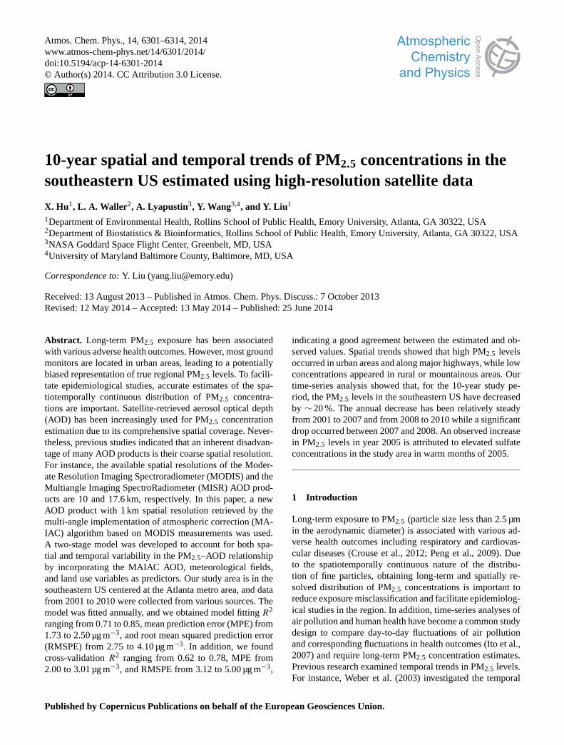
The study area is approximately 600× 600 km2 in the south-eastern US, covering most of Georgia, Alabama, and Ten-nessee, and parts of North and South Carolina (Fig. 1).The domain includes several large urban centers, numerousmedium-to-small cities, as well as suburban and rural areas.

2.2 PM2.5 measurements

The 24 h average PM2.5 concentrations from 2001 to 2010collected from the US EPA federal reference monitors(FRMs) were downloaded from the EPA’s Air QualitySystem Technology Transfer Network (http://www.epa.gov/ttn/airs/airsaqs/). PM2.5 concentrations less than 2 µg m−3

(∼ 0.2–3 % of total data records) were discarded as they arebelow the established limit of detection (EPA, 2008a).

2.3 Remote sensing data

MAIAC retrieves aerosol parameters over land at 1 km res-olution, which was accomplished by using the time seriesof MODIS measurements and simultaneous processing of agroup of pixels in fixed 25× 25 km2 blocks (Lyapustin et al.,2011a, b, 2012). MAIAC uses a sliding window to collect upto 16 days of MODIS radiance observations over the samearea and processes them to obtain surface parameters usedfor aerosol retrievals. To facilitate the time-series analysis,MODIS data are initially gridded to a 1 km resolution in aselected projection. For this work, we used MODIS level 1B(calibrated and geometrically corrected) data from Collec-tion 6 re-processing, which removed major effects of tem-poral calibration degradation of Terra and Aqua, a necessaryprerequisite for the trend analysis.

Validation based on the Aerosol Robotic Network(AERONET) data showed that MAIAC and the operationalCollection 5 MODIS Dark Target AOD have a similar ac-curacy over dark and vegetated surfaces, but also showedthat MAIAC generally improves accuracy over brighter sur-faces, including most urban areas (Lyapustin et al., 2011b).MAIAC AOD data from 2001 to 2010 were obtained fromthe National Aeronautics and Space Administration (NASA)Goddard Space Flight Center. Due to the lack of sufficientdata records from AERONET, a comparison between MA-IAC AOD and AERONET measurements in our study do-main was not possible.

Zhang et al. (2012) found that Terra and Aqua may pro-vide a good estimate of the daily average of AOD. Thus, theaverage of the Aqua and Terra measurements can be usedto predict daily PM2.5 concentrations. In this study, Aqua(overpasses at∼ 1:30 p.m. local time) and Terra (overpassesat ∼ 10:30 a.m. local time) MAIAC AOD values were firstcombined to improve spatial coverage. In our study domain,the increase in spatial coverage ranged from 30.2 to 72.4 %

for Aqua and from 17.2 to 26.3 % for Terra from 2001 to2010. In a common MAIAC pixel, there might be only oneMAIAC product from either Aqua or Terra, or both may bepresent. In the second case, when we combine them, the av-eraged value, as pointed out by Lee et al. (2012), is likely tobetter reflect daily aerosol loading, yet in the first case, AODas an indicator of PM2.5 abundance is biased towards the at-mospheric condition either in the morning or early afternoon.To estimate the missing AOD value, Lee et al. (2011) defineda simple ratio between averaged Terra and Aqua AOD. Inthis study, we fitted a linear regression to define the relation-ship between daily mean Terra-MAIAC and Aqua-MAIACAOD values. We used this regression to predict the missingAOD value (i.e., predict Terra-MAIAC AOD with the avail-able Aqua-MAIAC AOD, and vice versa), and then averagedthe observed and the predicted AOD values together. Finally,we set an upper bound of 2.0 for the combined AOD to re-duce potential cloud contamination (∼ 0.05–0.1 % of totaldata records were excluded).

2.4 Meteorological fields

The meteorological fields provided by the North AmericanLand Data Assimilation System (NLDAS) Phase 2 weredownloaded from the NLDAS website (http://ldas.gsfc.nasa.gov/nldas/). The spatial resolution of NLDAS meteorolog-ical data is 1/8th of a degree (∼ 13 km). Another meteoro-logical data set used in this study is the North AmericanRegional Reanalysis (NARR). NARR is a long-term, con-sistent, high-resolution climate data set for North America(Mesinger et al., 2006), with a spatial resolution of∼ 32 km.NLDAS provides most of the meteorological fields usedin this analysis, including relative humidity,U wind, andV wind, while NARR provides another critical parameter:boundary layer height. To generate daytime meteorologi-cal fields corresponding to the MODIS overpass times, 3-hourly NARR measurements and hourly NLDAS measure-ments from 10 a.m. to 4 p.m. standard local time were aver-aged.

2.5 Land use variables

Elevation data were downloaded from the national elevationdata set (NED) (http://ned.usgs.gov). NED is the seamless el-evation data set covering the conterminous United States andis distributed by the US Geological Survey (USGS). The ele-vation data are downloaded at a spatial resolution of 1 arcsec(∼ 30 m). The road data were obtained from ESRI StreetMapUSA (Environmental Systems Research Institute, Inc., Red-land, CA). The road data at level A1 (limited access highway)were extracted. Summed length of road segments was calcu-lated for each 1× 1 km2 MAIAC grid cell, and grid cells withno roads were assigned zero. The 2001 and 2006 Landsat-derived land cover maps covering the study area with a spa-tial resolution of 30 m were downloaded from the National

www.atmos-chem-phys.net/14/6301/2014/ Atmos. Chem. Phys., 14, 6301–6314, 2014

http://www.epa.gov/ttn/airs/airsaqs/

http://www.epa.gov/ttn/airs/airsaqs/

http://ldas.gsfc.nasa.gov/nldas/

http://ldas.gsfc.nasa.gov/nldas/

http://ned.usgs.gov


Figure 1. Study area.

Land Cover Database (NLCD) (http://www.mrlc.gov). For-est cover maps were generated by assigning one to forestpixels and zero to others. Primary PM2.5 emissions (tons peryear) were obtained from the 2002, 2005, and 2008 EPA Na-tional Emissions Inventory (NEI) facility emissions reports.Grid cells with multiple emission sources were assigned thesummed value, and those with no emissions were assignedzero.

2.6 Data integration

All the data were first re-projected to the USA Contigu-ous Albers Equal Area Conic USGS coordinate system. Formodel fitting, a 1× 1 km2 square buffer was generated foreach PM2.5 monitoring site. Meteorological fields and AODvalues were assigned to each PM2.5 monitoring site usingthe nearest neighbor approach. Forest cover and elevationwere averaged, while road length and point emissions weresummed over the 1× 1 km2 square buffer by calculating thetotal length of road segments and total point emissions withinthe buffer. For PM2.5 prediction, the same procedure was per-formed for each 1× 1 km2 MAIAC grid cell.

2.7 Model structure

We adopted the two-stage spatiotemporal model developedby Hu et al. (2014). For the model to be valid, we assumedthat particles within the boundary layer were well mixed,and the vertical distribution of particles above boundary layerwas relatively smooth. The first stage is a LME model withday-specific random intercepts and slopes for AOD and me-

teorological fields to account for the temporally varying re-lationship between observed PM2.5 and AOD (Eq. 1). Themodel structure can be expressed as

PM2.5,st = (b0 + b0,t ) + (b1 + b1,t )AODst + (b2 + b2,t )

MeteorologicalFieldsst + b3Elevations+ b4MajorRoadss+ b5ForestCovers+ b6PointEmissionss+ εst (b0,tb1,tb2,t ) ∼ N [(0,0,0) ,9] , (1)

wherebi andbi,t (day-specific) are the fixed and random in-tercept and slopes, respectively. Fixed intercepts and slopesare the same for all days and generated via conventional lin-ear regression, while random intercepts and slopes vary in-dependently for each individual day and are estimated vialikelihood methods from the full set of observations. In thisstudy, we generated fixed slopes for each predictor variable,but random slopes were only generated for AOD and meteo-rological fields, since they represent time-varying variables.The fixed slopes (e.g.,b1, b2, . . . ,b6) denote the overall rela-tionship for all days, and the random slopes (e.g.,b1,tb2,t ) in-dicate the daily relationship among PM2.5, AOD, and meteo-rological fields. PM2.5,st is the measured ground level PM2.5concentration (µg m−3) at sites on dayt ; AODst is the MA-IAC AOD value (unitless) at sites on day t ; Meteorolog-ical Fieldsst is the meteorological parameters at sites ondayt and may include Relative Humidityst , Boundary LayerHeightst , Wind Speedst , U Windst , andV Windst ; RelativeHumidityst is the relative humidity (%) at sites on day t ;Boundary Layer Heightst is the boundary layer height (m) atsites on dayt ; Wind Speedst is the 2 m wind speed (m s−1) atsites on dayt ; U Windst is the east–west component of wind


http://www.mrlc.gov


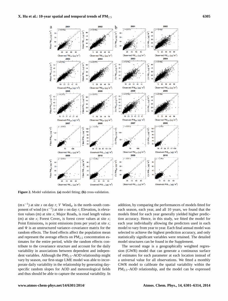
Figure 2. Model validation.(a) model fitting;(b) cross-validation.

(m s−1) at sites on dayt ; V Windst is the north–south com-ponent of wind (m s−1) at sites on dayt ; Elevations is eleva-tion values (m) at sites; Major Roadss is road length values(m) at sites; Forest Covers is forest cover values at sites;Point Emissionss is point emissions (tons per year) at sites;and9 is an unstructured variance–covariance matrix for therandom effects. The fixed effects affect the population meanand represent the average effects on PM2.5 concentration es-timates for the entire period, while the random effects con-tribute to the covariance structure and account for the dailyvariability in associations between dependent and indepen-dent variables. Although the PM2.5–AOD relationship mightvary by season, our first-stage LME model was able to incor-porate daily variability in the relationship by generating day-specific random slopes for AOD and meteorological fieldsand thus should be able to capture the seasonal variability. In

addition, by comparing the performances of models fitted foreach season, each year, and all 10 years, we found that themodels fitted for each year generally yielded higher predic-tion accuracy. Hence, in this study, we fitted the model foreach year individually allowing the predictors used in eachmodel to vary from year to year. Each final annual model wasselected to achieve the highest prediction accuracy, and onlystatistically significant variables were retained. The detailedmodel structures can be found in the Supplement.

The second stage is a geographically weighted regres-sion (GWR) model that can generate a continuous surfaceof estimates for each parameter at each location instead ofa universal value for all observations. We fitted a monthlyGWR model to calibrate the spatial variability within thePM2.5–AOD relationship, and the model can be expressed



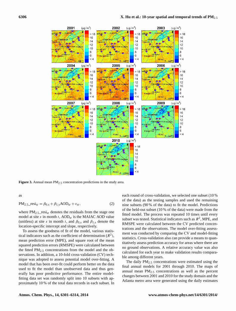
Figure 3. Annual mean PM2.5 concentration predictions in the study area.

as

PM2.5_resist = β0,s+ β1,sAODst + εst , (2)

where PM2.5_resist denotes the residuals from the stage onemodel at sites in montht , AODst is the MAIAC AOD value(unitless) at sites in month t , andβ0,s andβ1,s denote thelocation-specific intercept and slope, respectively.

To assess the goodness of fit of the model, various statis-tical indicators such as the coefficient of determination (R2),mean prediction error (MPE), and square root of the meansquared prediction errors (RMSPE) were calculated betweenthe fitted PM2.5 concentrations from the model and the ob-servations. In addition, a 10-fold cross-validation (CV) tech-nique was adopted to assess potential model over-fitting. Amodel that has been over-fit could perform better on the dataused to fit the model than unobserved data and thus gen-erally has poor predictive performance. The entire model-fitting data set was randomly split into 10 subsets with ap-proximately 10 % of the total data records in each subset. In

each round of cross-validation, we selected one subset (10 %of the data) as the testing samples and used the remainingnine subsets (90 % of the data) to fit the model. Predictionsof the held-out subset (10 % of the data) were made from thefitted model. The process was repeated 10 times until everysubset was tested. Statistical indicators such asR2, MPE, andRMSPE were calculated between the CV predicted concen-trations and the observations. The model over-fitting assess-ment was conducted by comparing the CV and model-fittingstatistics. Cross-validation also can provide a means to quan-titatively assess prediction accuracy for areas where there areno ground observations. A relative accuracy value was alsocalculated for each year to make validation results compara-ble among different years.

The daily PM2.5 concentrations were estimated using thefinal annual models for 2001 through 2010. The maps ofannual mean PM2.5 concentrations as well as the percentchanges between 2001 and 2010 for the study domain and theAtlanta metro area were generated using the daily estimates



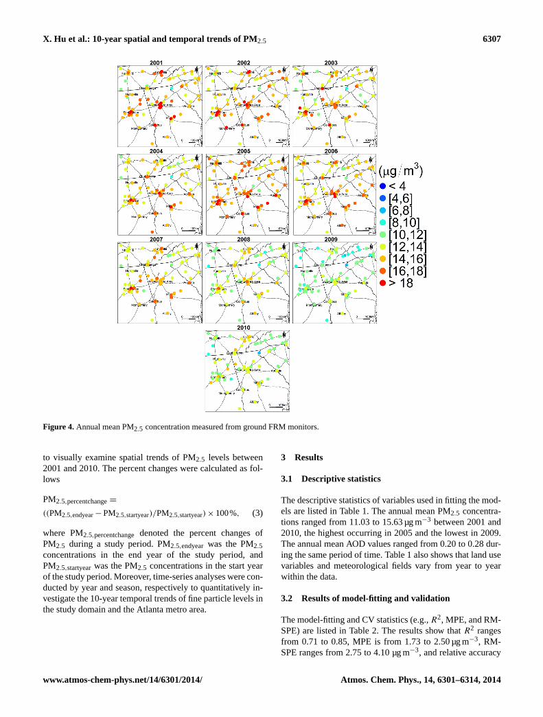
Figure 4. Annual mean PM2.5 concentration measured from ground FRM monitors.

to visually examine spatial trends of PM2.5 levels between2001 and 2010. The percent changes were calculated as fol-lows

PM2.5,percentchange=

((PM2.5,endyear− PM2.5,startyear)/PM2.5,startyear) × 100%, (3)

where PM2.5,percentchangedenoted the percent changes ofPM2.5 during a study period. PM2.5,endyear was the PM2.5concentrations in the end year of the study period, andPM2.5,startyearwas the PM2.5 concentrations in the start yearof the study period. Moreover, time-series analyses were con-ducted by year and season, respectively to quantitatively in-vestigate the 10-year temporal trends of fine particle levels inthe study domain and the Atlanta metro area.

3 Results

3.1 Descriptive statistics

The descriptive statistics of variables used in fitting the mod-els are listed in Table 1. The annual mean PM2.5 concentra-tions ranged from 11.03 to 15.63 µg m−3 between 2001 and2010, the highest occurring in 2005 and the lowest in 2009.The annual mean AOD values ranged from 0.20 to 0.28 dur-ing the same period of time. Table 1 also shows that land usevariables and meteorological fields vary from year to yearwithin the data.

3.2 Results of model-fitting and validation

The model-fitting and CV statistics (e.g.,R2, MPE, and RM-SPE) are listed in Table 2. The results show thatR2 rangesfrom 0.71 to 0.85, MPE is from 1.73 to 2.50 µg m−3, RM-SPE ranges from 2.75 to 4.10 µg m−3, and relative accuracy



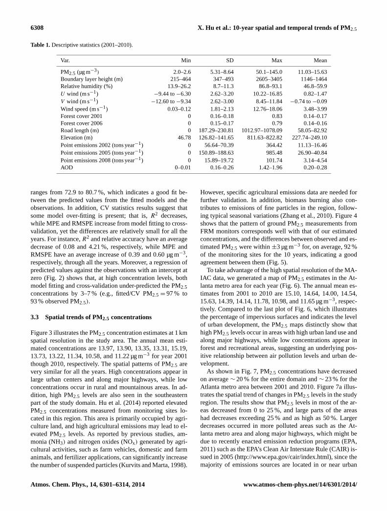
Table 1.Descriptive statistics (2001–2010).

Var. Min SD Max Mean

PM2.5 (µg m−3) 2.0–2.6 5.31–8.64 50.1–145.0 11.03–15.63Boundary layer height (m) 215–464 347–493 2605–3405 1146–1464Relative humidity (%) 13.9–26.2 8.7–11.3 86.8–93.1 46.8–59.9U wind (m s−1) −9.44 to−6.30 2.62–3.20 10.22–16.85 0.82–1.47V wind (m s−1) −12.60 to−9.34 2.62–3.00 8.45–11.84 −0.74 to−0.09Wind speed (m s−1) 0.03–0.12 1.81–2.13 12.76–18.06 3.48–3.99Forest cover 2001 0 0.16–0.18 0.83 0.14–0.17Forest cover 2006 0 0.15–0.17 0.79 0.14–0.16Road length (m) 0 187.29–230.81 1012.97–1078.09 58.05–82.92Elevation (m) 46.78 126.82–141.65 811.63–822.82 227.74–249.10Point emissions 2002 (tons year−1) 0 56.64–70.39 364.42 11.13–16.46Point emissions 2005 (tons year−1) 0 150.89–188.63 985.48 26.90–40.84Point emissions 2008 (tons year−1) 0 15.89–19.72 101.74 3.14–4.54AOD 0–0.01 0.16–0.26 1.42–1.96 0.20–0.28

ranges from 72.9 to 80.7 %, which indicates a good fit be-tween the predicted values from the fitted models and theobservations. In addition, CV statistics results suggest thatsome model over-fitting is present; that is,R2 decreases,while MPE and RMSPE increase from model fitting to cross-validation, yet the differences are relatively small for all theyears. For instance,R2 and relative accuracy have an averagedecrease of 0.08 and 4.21 %, respectively, while MPE andRMSPE have an average increase of 0.39 and 0.60 µg m−3,respectively, through all the years. Moreover, a regression ofpredicted values against the observations with an intercept atzero (Fig. 2) shows that, at high concentration levels, bothmodel fitting and cross-validation under-predicted the PM2.5concentrations by 3–7 % (e.g., fitted/CV PM2.5 = 97 % to93 % observed PM2.5).

3.3 Spatial trends of PM2.5 concentrations

Figure 3 illustrates the PM2.5 concentration estimates at 1 kmspatial resolution in the study area. The annual mean esti-mated concentrations are 13.97, 13.90, 13.35, 13.31, 15.19,13.73, 13.22, 11.34, 10.58, and 11.22 µg m−3 for year 2001though 2010, respectively. The spatial patterns of PM2.5 arevery similar for all the years. High concentrations appear inlarge urban centers and along major highways, while lowconcentrations occur in rural and mountainous areas. In ad-dition, high PM2.5 levels are also seen in the southeasternpart of the study domain. Hu et al. (2014) reported elevatedPM2.5 concentrations measured from monitoring sites lo-cated in this region. This area is primarily occupied by agri-culture land, and high agricultural emissions may lead to el-evated PM2.5 levels. As reported by previous studies, am-monia (NH3) and nitrogen oxides (NOx) generated by agri-cultural activities, such as farm vehicles, domestic and farmanimals, and fertilizer applications, can significantly increasethe number of suspended particles (Kurvits and Marta, 1998).

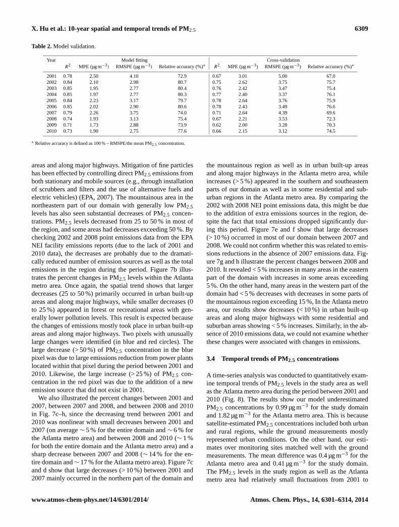
However, specific agricultural emissions data are needed forfurther validation. In addition, biomass burning also con-tributes to emissions of fine particles in the region, follow-ing typical seasonal variations (Zhang et al., 2010). Figure 4shows that the pattern of ground PM2.5 measurements fromFRM monitors corresponds well with that of our estimatedconcentrations, and the differences between observed and es-timated PM2.5 were within±3 µg m−3 for, on average, 92 %of the monitoring sites for the 10 years, indicating a goodagreement between them (Fig. 5).

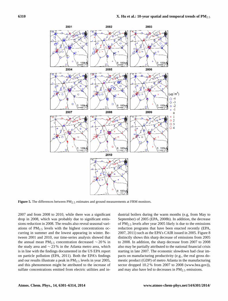
To take advantage of the high spatial resolution of the MA-IAC data, we generated a map of PM2.5 estimates in the At-lanta metro area for each year (Fig. 6). The annual mean es-timates from 2001 to 2010 are 15.10, 14.64, 14.00, 14.54,15.63, 14.39, 14.14, 11.78, 10.98, and 11.65 µg m−3, respec-tively. Compared to the last plot of Fig. 6, which illustratesthe percentage of impervious surfaces and indicates the levelof urban development, the PM2.5 maps distinctly show thathigh PM2.5 levels occur in areas with high urban land use andalong major highways, while low concentrations appear inforest and recreational areas, suggesting an underlying pos-itive relationship between air pollution levels and urban de-velopment.

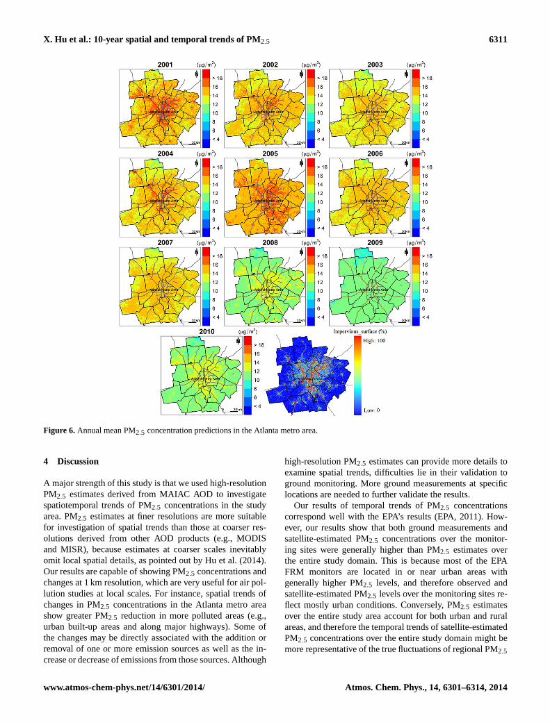
As shown in Fig. 7, PM2.5 concentrations have decreasedon average∼ 20 % for the entire domain and∼ 23 % for theAtlanta metro area between 2001 and 2010. Figure 7a illus-trates the spatial trend of changes in PM2.5 levels in the studyregion. The results show that PM2.5 levels in most of the ar-eas decreased from 0 to 25 %, and large parts of the areashad decreases exceeding 25 % and as high as 50 %. Largerdecreases occurred in more polluted areas such as the At-lanta metro area and along major highways, which might bedue to recently enacted emission reduction programs (EPA,2011) such as the EPA’s Clean Air Interstate Rule (CAIR) is-sued in 2005 (http://www.epa.gov/cair/index.html), since themajority of emissions sources are located in or near urban


http://www.epa.gov/cair/index.html


Table 2.Model validation.

Year Model fitting Cross-validationR2 MPE (µg m−3) RMSPE (µg m−3) Relative accuracy (%)∗ R2 MPE (µg m−3) RMSPE (µg m−3) Relative accuracy (%)∗

2001 0.78 2.50 4.10 72.9 0.67 3.01 5.00 67.02002 0.84 2.10 2.98 80.7 0.75 2.62 3.75 75.72003 0.85 1.95 2.77 80.4 0.76 2.42 3.47 75.42004 0.85 1.97 2.77 80.3 0.77 2.40 3.37 76.12005 0.84 2.23 3.17 79.7 0.78 2.64 3.76 75.92006 0.85 2.02 2.90 80.6 0.78 2.43 3.49 76.62007 0.79 2.26 3.75 74.0 0.71 2.64 4.39 69.62008 0.74 1.93 3.13 75.4 0.67 2.21 3.53 72.32009 0.71 1.73 2.88 73.9 0.62 2.00 3.28 70.32010 0.73 1.90 2.75 77.6 0.66 2.15 3.12 74.5

∗ Relative accuracy is defined as 100 % – RMSPE/the mean PM2.5 concentration.

areas and along major highways. Mitigation of fine particleshas been effected by controlling direct PM2.5 emissions fromboth stationary and mobile sources (e.g., through installationof scrubbers and filters and the use of alternative fuels andelectric vehicles) (EPA, 2007). The mountainous area in thenortheastern part of our domain with generally low PM2.5levels has also seen substantial decreases of PM2.5 concen-trations. PM2.5 levels decreased from 25 to 50 % in most ofthe region, and some areas had decreases exceeding 50 %. Bychecking 2002 and 2008 point emissions data from the EPANEI facility emissions reports (due to the lack of 2001 and2010 data), the decreases are probably due to the dramati-cally reduced number of emission sources as well as the totalemissions in the region during the period. Figure 7b illus-trates the percent changes in PM2.5 levels within the Atlantametro area. Once again, the spatial trend shows that largerdecreases (25 to 50 %) primarily occurred in urban built-upareas and along major highways, while smaller decreases (0to 25 %) appeared in forest or recreational areas with gen-erally lower pollution levels. This result is expected becausethe changes of emissions mostly took place in urban built-upareas and along major highways. Two pixels with unusuallylarge changes were identified (in blue and red circles). Thelarge decrease (> 50 %) of PM2.5 concentration in the bluepixel was due to large emissions reduction from power plantslocated within that pixel during the period between 2001 and2010. Likewise, the large increase (> 25 %) of PM2.5 con-centration in the red pixel was due to the addition of a newemission source that did not exist in 2001.

We also illustrated the percent changes between 2001 and2007, between 2007 and 2008, and between 2008 and 2010in Fig. 7c–h, since the decreasing trend between 2001 and2010 was nonlinear with small decreases between 2001 and2007 (on average∼ 5 % for the entire domain and∼ 6 % forthe Atlanta metro area) and between 2008 and 2010 (∼ 1 %for both the entire domain and the Atlanta metro area) and asharp decrease between 2007 and 2008 (∼ 14 % for the en-tire domain and∼ 17 % for the Atlanta metro area). Figure 7cand d show that large decreases (> 10 %) between 2001 and2007 mainly occurred in the northern part of the domain and

the mountainous region as well as in urban built-up areasand along major highways in the Atlanta metro area, whileincreases (> 5 %) appeared in the southern and southeasternparts of our domain as well as in some residential and sub-urban regions in the Atlanta metro area. By comparing the2002 with 2008 NEI point emissions data, this might be dueto the addition of extra emissions sources in the region, de-spite the fact that total emissions dropped significantly dur-ing this period. Figure 7e and f show that large decreases(> 10 %) occurred in most of our domain between 2007 and2008. We could not confirm whether this was related to emis-sions reductions in the absence of 2007 emissions data. Fig-ure 7g and h illustrate the percent changes between 2008 and2010. It revealed < 5 % increases in many areas in the easternpart of the domain with increases in some areas exceeding5 %. On the other hand, many areas in the western part of thedomain had < 5 % decreases with decreases in some parts ofthe mountainous region exceeding 15 %, In the Atlanta metroarea, our results show decreases (< 10 %) in urban built-upareas and along major highways with some residential andsuburban areas showing < 5 % increases. Similarly, in the ab-sence of 2010 emissions data, we could not examine whetherthese changes were associated with changes in emissions.

3.4 Temporal trends of PM2.5 concentrations

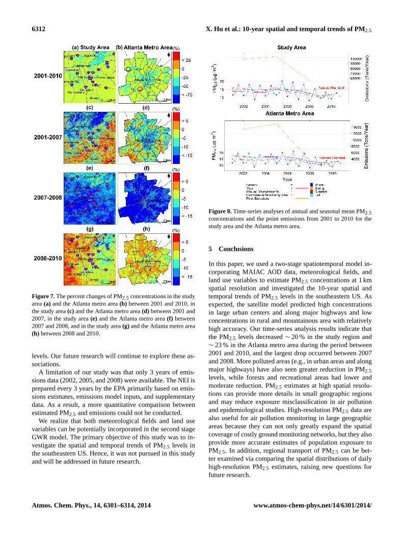
A time-series analysis was conducted to quantitatively exam-ine temporal trends of PM2.5 levels in the study area as wellas the Atlanta metro area during the period between 2001 and2010 (Fig. 8). The results show our model underestimatedPM2.5 concentrations by 0.99 µg m−3 for the study domainand 1.82 µg m−3 for the Atlanta metro area. This is becausesatellite-estimated PM2.5 concentrations included both urbanand rural regions, while the ground measurements mostlyrepresented urban conditions. On the other hand, our esti-mates over monitoring sites matched well with the groundmeasurements. The mean difference was 0.4 µg m−3 for theAtlanta metro area and 0.41 µg m−3 for the study domain.The PM2.5 levels in the study region as well as the Atlantametro area had relatively small fluctuations from 2001 to



Figure 5. The differences between PM2.5 estimates and ground measurements at FRM monitors.

2007 and from 2008 to 2010, while there was a significantdrop in 2008, which was probably due to significant emis-sions reduction in 2008. The results also reveal seasonal vari-ations of PM2.5 levels with the highest concentrations oc-curring in summer and the lowest appearing in winter. Be-tween 2001 and 2010, our time-series analysis showed thatthe annual mean PM2.5 concentration decreased∼ 20 % inthe study area and∼ 23 % in the Atlanta metro area, whichis in line with the findings documented in the US EPA reporton particle pollution (EPA, 2011). Both the EPA’s findingsand our results illustrate a peak in PM2.5 levels in year 2005,and this phenomenon might be attributed to the increase ofsulfate concentrations emitted from electric utilities and in-

dustrial boilers during the warm months (e.g, from May toSeptember) of 2005 (EPA, 2008b). In addition, the decreaseof PM2.5 levels after year 2005 likely is due to the emissionsreduction programs that have been enacted recently (EPA,2007, 2011) such as the EPA’s CAIR issued in 2005. Figure 8distinctly shows this sharp decrease of emissions from 2005to 2008. In addition, the sharp decrease from 2007 to 2008also may be partially attributed to the national financial crisisstarting in late 2007. The economic slowdown had clear im-pacts on manufacturing productivity (e.g., the real gross do-mestic product (GDP) of metro Atlanta in the manufacturingsector dropped 10.2 % from 2007 to 2008 (www.bea.gov)),and may also have led to decreases in PM2.5 emissions.


www.bea.gov


Figure 6. Annual mean PM2.5 concentration predictions in the Atlanta metro area.

4 Discussion

A major strength of this study is that we used high-resolutionPM2.5 estimates derived from MAIAC AOD to investigatespatiotemporal trends of PM2.5 concentrations in the studyarea. PM2.5 estimates at finer resolutions are more suitablefor investigation of spatial trends than those at coarser res-olutions derived from other AOD products (e.g., MODISand MISR), because estimates at coarser scales inevitablyomit local spatial details, as pointed out by Hu et al. (2014).Our results are capable of showing PM2.5 concentrations andchanges at 1 km resolution, which are very useful for air pol-lution studies at local scales. For instance, spatial trends ofchanges in PM2.5 concentrations in the Atlanta metro areashow greater PM2.5 reduction in more polluted areas (e.g.,urban built-up areas and along major highways). Some ofthe changes may be directly associated with the addition orremoval of one or more emission sources as well as the in-crease or decrease of emissions from those sources. Although

high-resolution PM2.5 estimates can provide more details toexamine spatial trends, difficulties lie in their validation toground monitoring. More ground measurements at specificlocations are needed to further validate the results.

Our results of temporal trends of PM2.5 concentrationscorrespond well with the EPA’s results (EPA, 2011). How-ever, our results show that both ground measurements andsatellite-estimated PM2.5 concentrations over the monitor-ing sites were generally higher than PM2.5 estimates overthe entire study domain. This is because most of the EPAFRM monitors are located in or near urban areas withgenerally higher PM2.5 levels, and therefore observed andsatellite-estimated PM2.5 levels over the monitoring sites re-flect mostly urban conditions. Conversely, PM2.5 estimatesover the entire study area account for both urban and ruralareas, and therefore the temporal trends of satellite-estimatedPM2.5 concentrations over the entire study domain might bemore representative of the true fluctuations of regional PM2.5



Figure 7.The percent changes of PM2.5 concentrations in the studyarea(a) and the Atlanta metro area(b) between 2001 and 2010, inthe study area(c) and the Atlanta metro area(d) between 2001 and2007, in the study area(e) and the Atlanta metro area(f) between2007 and 2008, and in the study area(g) and the Atlanta metro area(h) between 2008 and 2010.

levels. Our future research will continue to explore these as-sociations.

A limitation of our study was that only 3 years of emis-sions data (2002, 2005, and 2008) were available. The NEI isprepared every 3 years by the EPA primarily based on emis-sions estimates, emissions model inputs, and supplementarydata. As a result, a more quantitative comparison betweenestimated PM2.5 and emissions could not be conducted.

We realize that both meteorological fields and land usevariables can be potentially incorporated in the second stageGWR model. The primary objective of this study was to in-vestigate the spatial and temporal trends of PM2.5 levels inthe southeastern US. Hence, it was not pursued in this studyand will be addressed in future research.

Figure 8. Time-series analyses of annual and seasonal mean PM2.5concentrations and the point emissions from 2001 to 2010 for thestudy area and the Atlanta metro area.

5 Conclusions

In this paper, we used a two-stage spatiotemporal model in-corporating MAIAC AOD data, meteorological fields, andland use variables to estimate PM2.5 concentrations at 1 kmspatial resolution and investigated the 10-year spatial andtemporal trends of PM2.5 levels in the southeastern US. Asexpected, the satellite model predicted high concentrationsin large urban centers and along major highways and lowconcentrations in rural and mountainous area with relativelyhigh accuracy. Our time-series analysis results indicate thatthe PM2.5 levels decreased∼ 20 % in the study region and∼ 23 % in the Atlanta metro area during the period between2001 and 2010, and the largest drop occurred between 2007and 2008. More polluted areas (e.g., in urban areas and alongmajor highways) have also seen greater reduction in PM2.5levels, while forests and recreational areas had lower andmoderate reduction. PM2.5 estimates at high spatial resolu-tions can provide more details in small geographic regionsand may reduce exposure misclassification in air pollutionand epidemiological studies. High-resolution PM2.5 data arealso useful for air pollution monitoring in large geographicareas because they can not only greatly expand the spatialcoverage of costly ground monitoring networks, but they alsoprovide more accurate estimates of population exposure toPM2.5. In addition, regional transport of PM2.5 can be bet-ter examined via comparing the spatial distributions of dailyhigh-resolution PM2.5 estimates, raising new questions forfuture research.



The Supplement related to this article is available onlineat doi:10.5194/acp-14-6301-2014-supplement.

Acknowledgements.This work was partially supported byNASA Applied Sciences Program (grant no. NNX09AT52G andNNX11AI53G). In addition, this publication was made possible byUSEPA grant R834799. Its contents are solely the responsibility ofthe grantee and do not necessarily represent the official views ofthe USEPA. Further, USEPA does not endorse the purchase of anycommercial products or services mentioned in the publication.

Edited by: B. N. Duncan

References

Chudnovsky, A. A., Kostinski, A., Lyapustin, A., andKoutrakis, P.: Spatial scales of pollution from variable res-olution satellite imaging, Environ. Pollut., 172, 131–138,doi:10.1016/j.envpol.2012.08.016, 2012.

Crouse, D. L., Peters, P. A., van Donkelaar, A., Goldberg, M.S., Villeneuve, P. J., Brion, O., Khan, S., Atari, D. O., Jer-rett, M., Pope, C. A., Brauer, M., Brook, J. R., Martin, R.V., Stieb, D., and Burnett, R. T.: Risk of Non accidental andCardiovascular Mortality in Relation to Long-term Exposureto Low Concentrations of Fine Particulate Matter: A CanadianNational-Level Cohort Study, Environ. Health Persp., 120, 708–714, doi:10.1289/ehp.1104049, 2012.

EPA: lists of potential control measures for PM2.5 and precursors,Draft Version 1.0, U.S. Environmental Protection Agency, Of-fice of Air Quality Planning and Standards, Office of Trans-portation and Air Quality, Office of Atmospheric Programs, andOffice of Policy Analysis and Review,http://www.epa.gov/pm/measures/pm_control_measures_tables_ver1.pdf(last access: 20June 2014), 2007.

EPA: Quality assurance handbook for air pollution measurementsystems, Vollume II, Ambient Air Quality Monitoring Program.U.S. Environmental Protection Agency, Office of Air QualityPlanning and Standards, Air Quality Assessment Division, RTP,NC 27711, II, 2008a.

EPA: National Air Quality – Status and Trends through 2007. U.S.Environmental Protection Agency, Office of Air Quality Plan-ning and Standards, Air Quality Assessment Division, RTP, NC27711, 2008b.

EPA: National Air Quality – Status and Trends through 2010. U.S.Environmental Protection Agency, Office of Air Quality Plan-ning and Standards, Air Quality Assessment Division, RTP, NC27711, 2011.

Gupta, P. and Christopher, S. A.: Particulate matter air qualityassessment using integrated surface, satellite, and meteorolog-ical products: Multiple regression approach, J. Geophys. Res.-Atmos., 114, D14205, doi:10.1029/2008jd011496, 2009.

Hu, X., Waller, L. A., Al-Hamdan, M. Z., Crosson, W. L., Estes Jr.,M. G., Estes, S. M., Quattrochi, D. A., Sarnat, J. A., and Liu,Y.: Estimating ground-level PM2.5 concentrations in the south-eastern U.S. using geographically weighted regression, Environ.Res., 121, 1–10, doi:10.1016/j.envres.2012.11.003, 2013.

Hu, X., Waller, L. A., Lyapustin, A., Wang, Y., Al-Hamdan, M. Z.,Crosson, W. L., Estes Jr., M. G., Estes, S. M., Quattrochi, D. A.,Puttaswamy, S. J., and Liu, Y.: Estimating ground-level PM2.5concentrations in the Southeastern United States using MAIACAOD retrievals and a two-stage model, Remote Sens. Environ.,140, 220–232, doi:10.1016/j.rse.2013.08.032, 2014.

Ito, K., Thurston, G. D., and Silverman, R. A.: Characterization ofPM2.5, gaseous pollutants, and meteorological interactions in thecontext of time-series health effects models, J. Expo. Sci. Env.Epid., 17, S45–S60, 2007.

Kloog, I., Koutrakis, P., Coull, B. A., Lee, H. J., and Schwartz,J.: Assessing temporally and spatially resolved PM2.5 expo-sures for epidemiological studies using satellite aerosol op-tical depth measurements, Atmos. Environ., 45, 6267–6275,doi:10.1016/j.atmosenv.2011.08.066, 2011.

Kurvits, T. and Marta, T.: Agricultural NH3 and NOx emissionsin Canada, Environ. Pollut., 102, 187–194, doi:10.1016/S0269-7491(98)80032-8, 1998.

Lee, H. J., Liu, Y., Coull, B. A., Schwartz, J., and Koutrakis,P.: A novel calibration approach of MODIS AOD data to pre-dict PM2.5 concentrations, Atmos. Chem. Phys., 11, 7991–8002,doi:10.5194/acp-11-7991-2011, 2011.

Lee, H. J., Coull, B. A., Bell, M. L., and Koutrakis, P.: Use ofsatellite-based aerosol optical depth and spatial clustering to pre-dict ambient PM2.5 concentrations, Environ. Res., 118, 8–15,doi:10.1016/j.envres.2012.06.011, 2012.

Liu, Y., Franklin, M., Kahn, R., and Koutrakis, P.: Usingaerosol optical thickness to predict ground-level PM2.5 con-centrations in the St. Louis area: A comparison betweenMISR and MODIS, Remote Sens. Environ., 107, 33–44,doi:10.1016/j.rse.2006.05.022, 2007.

Liu, Y., Paciorek, C. J., and Koutrakis, P.: Estimating Regional Spa-tial and Temporal Variability of PM2.5 Concentrations UsingSatellite Data, Meteorology, and Land Use Information, Environ.Health Persp., 117, 886–892, doi:10.1289/ehp.0800123, 2009.

Lyapustin, A., Martonchik, J., Wang, Y. J., Laszlo, I., and Korkin,S.: Multiangle implementation of atmospheric correction (MA-IAC): 1. Radiative transfer basis and look-up tables, J. Geophys.Res.-Atmos., 116, D03210, doi:10.1029/2010jd014985, 2011a.

Lyapustin, A., Wang, Y., Laszlo, I., Kahn, R., Korkin, S., Remer,L., Levy, R., and Reid, J. S.: Multiangle implementation of atmo-spheric correction (MAIAC): 2. Aerosol algorithm, J. Geophys.Res.-Atmos., 116, D03211, doi:10.1029/2010jd014986, 2011b.

Lyapustin, A., Wang, Y., Laszlo, I., Hilker, T., Hall, F. G., Sell-ers, P. J., Tucker, C. J., and Korkin, S. V.: Multi-angle imple-mentation of atmospheric correction for MODIS (MAIAC): 3.Atmospheric correction, Remote Sens. Environ., 127, 385–393,doi:10.1016/j.rse.2012.09.002, 2012.

Mesinger, F., DiMego, G., Kalnay, E., Mitchell, K., Shafran, P. C.,Ebisuzaki, W., Jovic, D., Woollen, J., Rogers, E., and Berbery, E.H.: North American regional reanalysis, B. Am. Meteorol. Soc.,87, 343–360, 2006.

Paciorek, C. J., Liu, Y., Moreno-Macias, H., and Kondragunta,S.: Spatiotemporal associations between GOES aerosol opticaldepth retrievals and ground-level PM2.5, Environ. Sci. Technol.,42, 5800–5806, doi:10.1021/es703181j, 2008.

Peng, R. D., Bell, M. L., Geyh, A. S., McDermott, A., Zeger, S. L.,Samet, J. M., and Dominici, F.: Emergency Admissions for Car-diovascular and Respiratory Diseases and the Chemical Compo-


http://dx.doi.org/10.5194/acp-14-6301-2014-supplement

http://dx.doi.org/10.1016/j.envpol.2012.08.016

http://dx.doi.org/10.1289/ehp.1104049

http://www.epa.gov/pm/measures/pm_control_measures_tables_ver1.pdf

http://www.epa.gov/pm/measures/pm_control_measures_tables_ver1.pdf

http://dx.doi.org/10.1029/2008jd011496

http://dx.doi.org/10.1016/j.envres.2012.11.003

http://dx.doi.org/10.1016/j.rse.2013.08.032

http://dx.doi.org/10.1016/j.atmosenv.2011.08.066

http://dx.doi.org/10.1016/S0269-7491(98)80032-8

http://dx.doi.org/10.1016/S0269-7491(98)80032-8

http://dx.doi.org/10.5194/acp-11-7991-2011

http://dx.doi.org/10.1016/j.envres.2012.06.011



http://dx.doi.org/10.1029/2010jd014985

http://dx.doi.org/10.1029/2010jd014986


http://dx.doi.org/10.1021/es703181j


sition of Fine Particle Air Pollution, Environ. Health Persp., 117,957–963, doi:10.1289/ehp.0800185, 2009.

Prados, A. I., Kondragunta, S., Ciren, P., and Knapp, K. R.: GOESAerosol/Smoke Product (GASP) over North America: Compar-isons to AERONET and MODIS observations, J. Geophys. Res.,112, D15201, doi:10.1029/2006jd007968, 2007.

Schafer, K., Harbusch, A., Emeis, S., Koepke, P., and Wiegner, M.:Correlation of aerosol mass near the ground with aerosol opticaldepth during two seasons in Munich, Atmos. Environ., 42, 4036–4046, doi:10.1016/j.atmosenv.2008.01.060, 2008.

So, K. L., Guo, H., and Li, Y. S.: Long-term variation of PM2.5 lev-els and composition at rural, urban, and roadside sites in HongKong: Increasing impact of regional air pollution, Atmos. Envi-ron., 41, 9427–9434, doi:10.1016/j.atmosenv.2007.08.053, 2007.

van Donkelaar, A., Martin, R. V., Brauer, M., Kahn, R., Levy, R.,Verduzco, C., and Villeneuve, P. J.: Global Estimates of Ambi-ent Fine Particulate Matter Concentrations from Satellite-BasedAerosol Optical Depth: Development and Application, Environ.Health Persp., 118, 847–855, doi:10.1289/ehp.0901623, 2010.

Wallace, J., Kanaroglou, P., and Ieee: An investigation of air pol-lution in southern Ontario, Canada, with MODIS and MISRaerosol data, in: Igarss: 2007 Ieee International Geoscience andRemote Sensing Symposium, Vols 1–12 – Sensing and Under-standing Our Planet, IEEE International Symposium on Geo-science and Remote Sensing (IGARSS), Ieee, New York, 4311–4314, 2007.

Weber, R., Orsini, D., Duan, Y., Baumann, K., Kiang, C. S.,Chameides, W., Lee, Y. N., Brechtel, F., Klotz, P., Jongejan, P.,ten Brink, H., Slanina, J., Boring, C. B., Genfa, Z., Dasgupta, P.,Hering, S., Stolzenburg, M., Dutcher, D. D., Edgerton, E., Hart-sell, B., Solomon, P., and Tanner, R.: Intercomparison of nearreal time monitors of PM2.5 nitrate and sulfate at the US En-vironmental Protection Agency Atlanta Supersite, J. Geophys.Res.-Atmos., 108, 8421, doi:10.1029/2001jd001220, 2003.

Zeger, S. L., Thomas, D., Dominici, F., Samet, J. M., Schwartz,J., Dockery, D., and Cohen, A.: Exposure measurement error intime-series studies of air pollution: concepts and consequences,Environ. Health Persp., 108, 419–426, doi:10.2307/3454382,2000.

Zhang, X., Hecobian, A., Zheng, M., Frank, N. H., and Weber, R.J.: Biomass burning impact on PM2.5 over the southeastern USduring 2007: integrating chemically speciated FRM filter mea-surements, MODIS fire counts and PMF analysis, Atmos. Chem.Phys., 10, 6839–6853, doi:10.5194/acp-10-6839-2010, 2010.

Zhang, Y., Yu, H., Eck, T. F., Smirnov, A., Chin, M., Remer, L.A., Bian, H., Tan, Q., Levy, R., Holben, B. N., and Piazzolla,S.: Aerosol daytime variations over North and South Americaderived from multiyear AERONET measurements, J. Geophys.Res.-Atmos., 117, D05211, doi:10.1029/2011jd017242, 2012.



http://dx.doi.org/10.1029/2006jd007968




http://dx.doi.org/10.1029/2001jd001220

http://dx.doi.org/10.2307/3454382

http://dx.doi.org/10.5194/acp-10-6839-2010

http://dx.doi.org/10.1029/2011jd017242

10-year spatial and temporal trends of pm concentrations...

Documents