1584 ieee transactions on smart grid, vol. 7, no. 3, may

1584 IEEE TRANSACTIONS ON SMART GRID, VOL. 7, NO. 3, MAY 2016

Proactive Demand Response for Data Centers:A Win-Win Solution

Hao Wang, Student Member, IEEE, Jianwei Huang, Senior Member, IEEE, Xiaojun Lin, Senior Member, IEEE,and Hamed Mohsenian-Rad, Senior Member, IEEE

Abstract—In order to reduce the energy cost of data centers,recent studies suggest distributing computation workload amongmultiple geographically dispersed data centers by exploiting theelectricity price difference. However, the impact of data centerload redistribution on the power grid is not well understood yet.This paper takes the first step toward tackling this importantissue by studying how the power grid can take advantage ofthe data centers’ load distribution proactively for the purposeof power load balancing. We model the interactions betweenpower grid and data centers as a two-stage problem where theutility company chooses proper pricing mechanisms to balancethe electric power load in the first stage and the data centersseek to minimize their total energy cost by responding to theprices in the second stage. We show that the two-stage problemis a bilevel quadratic program, which is NP-hard and cannot besolved using standard convex optimization techniques. We intro-duce benchmark problems to derive upper and lower boundsfor the solution of the two-stage problem. We further propose abranch and bound algorithm to attain the globally optimal solu-tion, and propose a heuristic algorithm with low computationalcomplexity to obtain an alternative close-to-optimal solution. Wealso study the impact of background load prediction error usingthe theoretical framework of robust optimization. The simula-tion results demonstrate that our proposed scheme can not onlyimprove the power grid reliability, but also reduce the energycost of data centers.

Index Terms—Smart grid, data center, demand response,dynamic electricity pricing, load balancing, proactive design.

Manuscript received October 31, 2014; revised May 13, 2015, August 6,2015, and September 27, 2015; accepted October 31, 2015. Date of pub-lication December 31, 2015; date of current version April 19, 2016. Thiswork was supported in part by the Research Grants Council of the HongKong Special Administrative Region, China, through Theme-Based ResearchScheme under Project T23-407/13-N, and in part by the National ScienceFoundation under Grant CCF-1442726, Grant ECCS-1509536, Grant CNS-1319798, Grant ECCS-1253516, and Grant ECCS-1307756. Part of the resultshave appeared in ACM GreenMetrics 2013 [1]. Paper no. TSG-01086-2014.(Corresponding author: Jianwei Huang.)

H. Wang and J. Huang are with the Network Communications andEconomics Laboratory, Department of Information Engineering, ChineseUniversity of Hong Kong, Hong Kong (e-mail: [email protected];[email protected]).

X. Lin is with the School of Electrical and Computer Engineering, PurdueUniversity, West Lafayette, IN 47907 USA (e-mail: [email protected]).

H. Mohsenian-Rad is with the Department of Electrical Engineering,University of California, Riverside, CA 92521 USA (e-mail:[email protected]).

Color versions of one or more of the figures in this paper are availableonline at http://ieeexplore.ieee.org.

Digital Object Identifier 10.1109/TSG.2015.2501808

NOMENCLATURE

Abbreviations

PS1 Stage-1 problemPS2 Stage-2 problemPI Integrated problemRS1 Stage-1 of the restricted problemRS2 Stage-2 of the restricted problemPE1 Equivalent problem of the Stage-1 problemPE2 Equivalent problem of the Stage-2 problemPR1 Relaxed Stage-1 problemWCP Worst-case performance optimization problem

Sets

T Set of time slotsN Set of data centers

Indices

t Index of time slotsi Index of data centers

Parameters

T Number of time slotsN Number of data centersLt Total incoming workload within time slot tMi Total number of servers in data center iμi Service rate of servers in data center idt

i Transmission delay to data center i in time slot tD Delay boundPidle Average idle power of serverPpeak Average peak power of serverRi Power usage effectiveness of data center iξi Base energy consumption of data center iαt

i Base price for data center i in time slot tβi Sensitivity parameter of price for data center iQt

i Available supply to data center i in time slot tBt

i Background load in location i and time slot tCi Power capacity in location iπ t

i Price lower bound for data center i in time slot tπ t

i Price upper bound for data center i in time slot tπ t

max Maximum average price in time slot tθi Coefficient for energy consumption of data center iEt Total energy required in time slot tEt

i Energy lower bound for data center i in time slot tE

ti Energy upper bound for data center i in time slot t

1949-3053 c© 2015 IEEE. Personal use is permitted, but republication/redistribution requires IEEE permission.See http://www.ieee.org/publications_standards/publications/rights/index.html for more information.

WANG et al.: PROACTIVE DEMAND RESPONSE FOR DATA CENTERS 1585

�ti,min Error lower bound in location i and time slot t

�ti,max Error upper bound in location i and time slot t

Variables

λti Workload assigned to data center i in time slot t

xti Number of active servers in data center i and time t

eti Energy consumption of data center i in time slot t

sti Billing reference for data center i in time slot t

π ti Unit energy price for data center i in time slot t

rti Electric load ratio in location i and time slot t

zti Auxiliary variables

zti Auxiliary variables

δti Load prediction error in location i and time slot t

I. INTRODUCTION

ENERGY management of large and distributed data cen-ters has become an increasingly important problem. With

the fast development of cloud computing services, it is nowcommon for a cloud provider (e.g., Google, Microsoft, andAmazon) to build multiple, large, and geographically dis-persed data centers across the continent. Each data centermay include hundreds of thousands of servers, massive stor-age equipment, cooling facilities, and power transformers. Theenergy consumption and cost of data centers hence can be sig-nificant [2]. For example, Google reported in 2011 that its datacenters continuously draw almost 260 MW of power, whichis more than what Salt Lake City consumes [3]. Microsoft’sdata center in Washington US consumes 48 MW of power,which is equivalent to the power consumption of about 40,000households. This has motivated growing research activitiestoward optimizing the data center operations to reduce thetotal energy cost. For example, Qureshi et al. in [2] proposedan energy cost minimization method for distributed data cen-ters to exploit electricity price difference. The idea is laterextended in [4]–[10].

However, most existing studies of energy management ofdistributed data centers have focused on the energy cost min-imization from the viewpoint of data centers, but failed toconsider the impact of such energy management practice onthe power grid. Note that, due to their enormous energy con-sumption, data centers are expected to have a great influenceon the operation of the power grid [11]. Without taking suchimpact into account, these energy management schemes mayadversely affect power-grid stability and load balancing.

In this paper, we aim to study the energy cost minimiza-tion of distributed data centers based on their impact to thepower grid. We seek to benefit from the recent advances intwo-way communications that are available in smart grid [12]to allow interactions and coordinations between energy sup-pliers and consumers in real time to improve demand sidemanagement. In our proposed framework, the utility companycan set dynamic prices to the demand-responsive data centers,and the data centers can dynamically change energy consump-tion in response to the price changes. This can effectivelycoordinate demand with supply, and hence avoid unintendedpower overloading.

Fig. 1. Smart grid and data center interaction.

The overall framework of our proposed system setup isshown in Fig. 1. Cloud service users send computing requestsvia Internet to the cloud provider. Exploiting various electric-ity prices at different locations, the cloud provider minimizesthe total energy cost by assigning users’ requests to differentdata centers. The utility company utilizes the demand responseof data centers, and tries to achieve power load balancing byaltering the electricity consumption of data centers throughdynamic pricing.

The main contributions of this paper are as follows:• Data center and smart grid interaction: To the best of

our knowledge, this is the first paper that studies theinteractions between smart grid and data centers by con-sidering the active decisions on both sides. In particular,how does the utility company properly incentivize datacenters to provide demand response services toward areliable power grid?

• Modeling and solution methods: We formulate the inter-actions between smart grid and data centers as a two-stage price optimization problem. In its original form,this problem cannot be solved by standard convex pro-gramming techniques. Therefore, we reformulate theproblem as a mixed integer quadratic program, anddesign a customized branch-and-bound algorithm to attainthe globally optimal solution. We also design a low-complexity descent algorithm to attain a close-to-optimalsolution.

• Performance benchmarks: To help characterizing theoptimal solution of the two-stage price optimizationproblem, we construct two single-level optimization prob-lems, namely an Integrated Problem and a RestrictedProblem, which correspond to the performance upperand lower bounds of the two-stage price optimizationproblem.

• Case studies and implications: Our proposed method cannot only balance the power load for smart grid but alsoreduce total energy cost for data centers, hence achievinga win-win result.

The remainder of the this paper is organized as follows.We review the related work in Section II. After that, weformulate the system model as a two-stage price optimiza-tion problem in Section III. In Section IV, we study twobenchmark problems to provide performance bounds for theformulated two-stage price optimization problem. In Section V,we analyze the solution of the two-stage price optimizationproblem, design a branch-and-bound algorithm to yield theglobal optimum, and propose an alternative heuristic algorithm


to solve the sub-optimal solution. In Section VI, we ana-lyze the worst-case performance by considering the predictionerror in background power load. Performance of the proposedscheme is evaluated in Section VII. This paper is concludedin Section VIII.

II. RELATED WORK AND MOTIVATION

A. Literature Review

There are many existing research results on managingdata center’s workload to reduce energy cost, such as thosestudying the energy cost minimization problem with multi-electricity-market environment [4], green renewable genera-tors [5], online optimization [6], service level agreements [7],and deregulated electricity price [8]. Zhang et al. [9] designeda Vickrey-Clarke-Groves auction mechanism, in which ten-ants of data centers voluntarily bid for emergency demandresponse. However, these results did not consider the activeresponse by the utility companies, nor did they consider howthe data centers’ demand response may bring large load fluc-tuations across different locations over time. This motivatesus to study the interactions between smart grid and geograph-ically dispersed data centers, and examine how smart grid canproperly incentivize data centers through dynamic pricing toimprove the grid reliability.

There has been a large body of research on demand responseof strategic energy consumers [13]–[16]. For example, in [13],Mohsenian-Rad and Leon-Garcia suggested scheduling house-hold devices based on the predicted prices to minimize theelectricity cost. In [14], Nguyen et al. proposed a game the-oretic model, in which an electricity provider dynamicallyupdates the energy prices to reduce the peak load, by con-sidering the load profiles of users. In [15], Li et al. studieddemand response based on utility maximization, and proposeda distributed algorithm to compute optimal prices and powerschedules. In [16], Joe-Wong et al. designed a time-dependentprice to incentivize users to shift power load so as to relievestress during peak hours.

B. Motivation

Different from traditional residential or industrial con-sumers, data centers are special electricity consumers. Thisis not only because of their enormous energy consumption,but also because of flexibility of energy consumptions overmultiple locations. The previous studies in [4]–[9] mainlyfocused on the workload distribution from the perspective ofdata centers. As reported in [10], such workload distributionof data centers has great impact on power load balancing inthe smart grid.

In the power system, the utility company is responsiblefor supplying power to meet the demand, and for maintain-ing the secure operation of the smart grid system. The utilitycompany can utilize the demand response of data centersto manage their energy consumption. However, most of theexisting demand response programs focused on the time flexi-bility of residential demands, without considering the demandside management over multiple locations. The latter is dif-ficult to do for residential demands, but is very suitable in

Fig. 2. The architecture for data center demand response.

the case of geographically dispersed data centers.1 This moti-vates us to design the dynamic pricing incentive mechanismfrom the grid operator’s point of view, in order to incentivizethe proper demand response from multiple geographically dis-persed data centers. Tran et al. [17] studied demand responseof data centers in a multi-utilities environment, and mod-eled the interactions between utilities and data centers as aStackelberg game. Different from [17], we study the interac-tion between one utility company and one cloud provider (withmultiple data centers) as a bi-level optimization problem, pro-pose two benchmark problems to estimate the performancebounds, and propose two algorithms to solve the optimal pricesand close-to-optimal prices, respectively.

III. SYSTEM MODEL

We consider a discrete time model t ∈ T = {1, . . . , T},where the length of a time slot matches the time-scale at whichthe workload allocation decisions and dynamic pricing deci-sions are updated, e.g., once an hour [4]. Let N = {1, . . . , N}denote the set of geographically dispersed data centers, whereeach data center i ∈ N has Mi homogeneous servers, andhas the same function in terms of supporting various kinds ofapplications (e.g., Internet services, image processing). As wewill explain later, not all servers are turned on during eachtime slot.

Fig. 2 illustrates the system architecture of data centers andsmart grid. We assume that a group of geographically dis-persed data centers are operated by a single cloud provider,and there is a traffic aggregator (e.g., a front-end portalserver) responsible for distributing the total incoming comput-ing workload Lt within time slot t to data centers in differentregions [4]. Each data center is powered by a dedicated powersubstation in the power grid, and all the substations are oper-ated by the same utility company.2 In each time slot t, wemodel the interactions between utility company and data cen-ters in two stages. In Stage 1, the utility company sets a billing

1The cloud provider owns multiple data centers located in different geo-graphical locations, and thus gains flexibility of power loads over locationsvia workload assignment over different data centers. As an example, whenGoogle responds to a user’s Web search query, the corresponding computa-tion can be done in any of the Google’s data centers (as long as certain servicequality agreement is satisfied).

2Many practical examples motivates our assumption of one utility company.For example, Alibaba cloud, a Chinese cloud provider, runs five data centersat different locations in China, and three of which are served by the StateGrid Corporation of China. Such scenarios also exist in deregulated electricitymarkets, such as in California US [18].


reference sti, which determines the electricity tariff as we will

explain later for each data center i to balance the load onthe power grid. In Stage 2, we assume that the data centerscan predict the workload accurately at the beginning of eachtime slot. Then data centers cooperate with each other (as theybelong to the same cloud operator) so as to minimize the totalenergy cost by determining the computing workload allocationλt

i and the number of active servers xti in each data center i.

Next, we discuss these decisions in details.

A. Stage 2: Data Center’s Energy Cost Minimization

First, we consider the Stage-2 problem, where a cloudprovider (such as Google) wants to minimize the total energycost of multiple data centers. In practice, data centers directlynegotiate with the utility company regarding the electricityrates [19]. In time slot t, the utility company charges datacenter i with the following regional electricity price π t

i perunit of energy:

π ti = αt

i + βi(eti − st

i), (1)

where eti is the data center’s the electricity consumption, st

i iscalled the billing reference, βi > 0 is a sensitivity parameter,and αt

i > 0 denotes the base price, all at location i in timeslot t. The dynamic pricing scheme in (1) is motivated by thetiered electricity pricing, which has been widely implementedin various power markets such as the United States, Japan, andChina. The key idea of tiered pricing is to set several pricingtiers for the energy consumption, and the unit price per unitof energy increases with the tiers progressively [20]. In (1),the term βi(et

i − sti) reflects the difference between electricity

consumption eti and the billing reference st

i. The unit price π ti

will be higher than the base price if eti > st

i.Next, we discuss the data centers’ optimization constraints.1) Workload Constraint: In each time slot t, users’ com-

puting requests (workload to the cloud provider) are receivedby a front-end portal server. Then a total of N data centersshould work together to complete the total workload of Lt,with the allocation to data center i as λt

i:

N∑

i=1

λti = Lt, λt

i ≥ 0, ∀i ∈ N , t ∈ T . (2)

2) QoS (Delay) Constraint: It is important for data centersto provide QoS guarantees to the users, and QoS can be spec-ified by the service level agreement (SLA) [21]. SLA usuallymeasures the average performance for the operation of a datacenter during a period of time. We consider both the transmis-sion delay (incurred before the request arrives at a data center)and the queuing delay (experienced after the request arrives ata data center). We define dt

i as the transmission delay expe-rienced by a computing request from the aggregator to datacenter i during time slot t. Notice that dt

i is usually much lessthan the length of a time slot. To model the queuing delay, weuse queuing theory to estimate the average processing time indata center i when there are xt

i active servers processing work-load λt

i with a service rate μi per server.3 Applying the results

3We assume that the servers in the same data center i are homogeneousand have the same service rate μi.

from M/M/1 queuing theory [5], the average waiting time isapproximately 1

μixti−λt

i. To meet the QoS requirement, the total

time delay experienced by a computing request should satisfysome delay bound D, which is the maximum waiting timethat a request can tolerate. For simplicity, in this paper, wewill assume homogeneous requests that have the same delaybound D. Therefore, we have the following QoS constraint

dti +

1

μixti − λt

i≤ D, ∀i ∈ N , t ∈ T , (3)

where μixti > λt

i.3) Server Constraint: At each data center i, there are tens

of thousands of servers providing cloud computing servicesto meet users’ requests. Let Mi denote the maximum numberof available servers. The cloud provider can switch on andoff servers to adjust the service time. Since the number ofservers is usually large, we can relax the integer constrainton the number of active servers without significantly affectingthe optimal result. Therefore, we have the following serverconstraint4

0 ≤ xti ≤ Mi, ∀i ∈ N , t ∈ T . (4)

4) Energy Consumption Constraint: The energy consump-tion of data centers consists of IT energy consumption(e.g., CPU, memory, and storage) and ancillary energy con-sumption (e.g., cooling, lighting, and power facility). Thequantitative relation between IT energy consumption andancillary energy consumption is measured by the power usageefficiency (PUE) [22], which is defined as the ratio of totalenergy consumption to IT energy consumption. The energyused by computing equipments is considered to be produc-tive. On the contrary, the energy for ancillary infrastructure(e.g., cooling, lighting, and power facility) is auxiliary. PUEhelps us understand the total energy consumption based on theIT energy consumption. Therefore, we can calculate the totalenergy consumption of a data center using PUE, amount ofcomputing workload, and number of active servers. Precisely,based on the data center power model in [11], we formulatethe energy consumption of data center i in time slot t as

eti = xt

i

(Pidle + (Ri − 1)Ppeak

)+ xti(Ppeak − Pidle)γ

ti + ξi,

where Pidle and Ppeak represent the average idle power andaverage peak power of a single server, respectively. The powerefficiency parameter Ri > 1 denotes PUE of data center i. Theparameter ξi is an empirical constant indicating the base energyconsumption of data center i, and γ t

i denotes the average serverutilization of data center i in time slot t.

We substitute the average server utilization γ ti = λt

i/(μixti),

and rewrite eti in the following equivalent form:

eti =

(Pidle + (Ri − 1)Ppeak

)xt

i +Ppeak − Pidle

μiλt

i + ξi,

∀i ∈ N , t ∈ T ,

(5)

4We set the minimum required number of active servers in each data centeras zero. It can also be set as a positive number to reflect operational require-ments for the data center, without changing the engineering insights from theanalysis.


which is an affine function with respect to the number of activeservers xt

i and the computing workload λti.

Given the operational requirements of the power substation,we limit the maximum power that can be consumed by datacenter i in time slot t as

0 ≤ eti ≤ Qt

i, ∀i ∈ N , t ∈ T , (6)

where Qti denotes the available power supply to data center i

in time slot t.With the above constraints, we can formulate the cloud

provider’s energy cost minimization problem in Stage 2. Theobjective is to minimize the data centers’ total energy costover all locations and all time slots by choosing the workloadallocation λt

i and the number of active servers xti for each data

center i ∈ N and each time t ∈ T . As the operational con-straints (2)-(6) are decoupled across time slots, we formulatethe energy cost minimization problem in time slot t as follows:

Stage-2 Problem (PS2): Total Energy Cost Minimization

minλt, xt

∑

i∈N

(αt

i + βi(eti − st

i))

eti

subject to Constraints (2)–(6),

where λt = {λti, ∀i ∈ N } and xt = {xt

i, ∀i ∈ N } denote theworkload allocation vector and active server number vectorfor each time slot t ∈ T , respectively. The energy cost of datacenter i is calculated as the product of its energy consumptionet

i and the corresponding unit price αti + βi(et

i − sti).

Note that, the optimal value of workload allocation λti, num-

ber of active servers xti and energy consumption et

i in (5) arefunctions of the billing references st = {st

i, ∀i ∈ N } in timeslot t. Given st, we can solve Problem PS2, and will presentthe optimal solutions of λt

i, xti and et

i in Section V.

B. Stage 1: Smart Grid’s Power Load Balancing Problem

We are now ready to consider the Stage-1 power load bal-ancing problem for the smart grid. We classify the load intotwo groups: data centers and others. We focus on the datacenters’ loads as they have geographical flexibility, and letthe latter group as background loads. With the emergence ofsmart grid communications technologies, it is possible for theutility company to incentivize the data centers to shift loadsfrom heavily loaded regions to lightly loaded regions. In ourproposed framework, the smart grid optimizes dynamic tieredprices by setting the billing references st in each time slot tto balance power load across geographical locations. To mea-sure the power load levels in different locations, we define theelectric load ratio in location i and time slot t as

rti(s

t) = eti(s

t)+ Bti

Ci, (7)

where Bti is the background power load, and Ci is the capacity

of power substation i. Note that the load ratio rti is a function

of the energy consumption eti, and thus also depends on the

billing reference st for all locations in time slot t. The utilitycompany aims at balancing the load ratio rt

i(st) at all locations

in each time slot.

Let Qti = Ci − Bt

i be the maximum available power supplyto data center i in time slot t. Since our study focuses onthe demand response of data centers, we denote the aggregateenergy usage of all the users other than data centers as thebackground energy load. We assume that the utility company isable to accurately forecast5 the background energy load aheadof each time slot [23].

Based on the load ratio rti , we define the electric load

index (ELI) across all locations in time slot t as

ELI �∑

i∈N

(rt

i(st))2

Ci, (8)

where ELI measures the overall load ratio across all loca-tions. Note that electric load ratio rt

i is a normalized indicator,which does not reflect the importance of those locations withlarge capacities. Therefore, we introduce the capacities Ci

as the weighted coefficients in ELI. We can show that min-imizing ELI with respect to et

i yields an equal load ratioacross all locations in the ideal case (without considering anyconstraints):

et1 + Bt

1

C1= · · · = et

N + BtN

CN,

which indicates no overloading problem occurs in any of thelocations. Therefore, the system reliability is improved at theselocations.

However, such even load distribution may not be achiev-able in practice, because the energy consumption et

i shouldalso satisfy the operational constraints for workload alloca-tion and number of active servers in (2)–(6). Moreover, thecloud provider and the utility company are independent enti-ties. Data centers are operated by the cloud provider, whichimplies that the energy consumption of data centers cannot bedirectly controlled by the utility company.

In order to balance the electricity load, in this paper wefocus on the scenario where the utility company chargesdynamic prices to incentivize users to shift their electricityusage to less loaded locations. To encourage the participa-tion of data centers into the demand response program andprevent the utility company from abusing its market power,constraints should be set to regulate the dynamic prices. Inpractice, the utility company and data centers usually negoti-ate with each other and enter into a contract [19] to specifythe pricing structure. Based on related studies [24], we set thefollowing constraints for the energy price π t

i :

π ti ≤ αt

i + βi(eti − st

i) ≤ π ti, ∀i ∈ N , t ∈ T , (9)

1

N

∑

i∈N

[αt

i + βi(eti − st

i)] ≤ π t

max, t ∈ T , (10)

where (9) ensures that the price charged to the data cen-ters is always contained within the range [π t

i, πti]. Constraint

(10) enforces that the dynamic prices across all locationshave an average price ceiling π t

max, which is specified by thecontract between the utility company and data centers [24].Constraint (10) can prevent the utility company from charging

5We first solve the two-stage problem assuming perfect background loadprediction. In Section VI, we will further study the impact of prediction error.


the maximum possible price in all locations. More precisely,the utility company has to provide lower prices to otherlocations if it charges a higher prices at some locations, sothat (10) can be satisfied. This will give a guarantee to thecloud provider, such that the dynamic price will not arbitrarilyincrease the energy cost of the data centers.

After the contract terms (e.g., constraints (9) and (10)) aresettled, the utility company is responsible for enforcing theprice constraints (9) and (10).6 We formulate the smart grid’sload balancing problem in time slot t as follows:

Stage-1 Problem (PS1): Electric Power Load Balancing

minst

∑

i∈N

(rt

i(st))2

Ci

subject to Constraints (9) and (10),

where the electric load ratio rti depends on the energy

consumption eti, which is the optimal solution of Stage-2

Problem PS2.

C. Two-Stage Price Optimization Problem

For Problem PS2, we can show that constraints (2)–(6) canbe equivalently rewritten as constraints of data centers’ energyconsumption:

∑

i∈Nθie

ti = Et, (11)

Eti ≤ et

i ≤ Eti, ∀i ∈ N , (12)

where θi, Et, Eti and E

ti are system parameters. Constraint (11)

is derived from the workload constraint in (2), which specifiesthat the summation of θi-weighed energy consumption of allthe data centers should reach Et in order to process the totalworkload Lt. The box constraint (12) sets the energy consump-tion lower bound Et

i and upper bound Eti for each data center,

to meet all the inequality constrains in (3)–(6). For the proofand detailed representation of the parameters, please see [33].

Using constraints (11) and (12), we can simplify ProblemPS2 into an equivalent energy consumption distribution prob-lem, in which the cloud provider directly decides the energyconsumption of data center et

i to minimize the energy cost.The equivalent energy consumption distribution problem ispresented as follows:

PE2: Equivalent Problem of PS2

minet

∑

i∈N

(αt

i + βi(eti − st

i))

eti


where et = {eti, ∀i ∈ N }. Once the energy consumption et

i isdetermined, we can find the corresponding workload allocationλt

i and number of active servers xti.

Fig. 3 shows the relation between the two-stage problemsPS1 and PE2, each of which is executed once in each time slot.

6To enforce constraints (9) and (10), the utility company should carefullydetermine the dynamic prices and consider the corresponding responses fromthe data centers, as the price constraints (9) and (10) involve both dynamicprices and energy consumption responses of data centers.

Fig. 3. Two-stage optimization problem.

In Stage 1, at the beginning of each time slot, the utility com-pany sets billing references for data centers to optimize the ELIperformance. This leads to the tiered price π t

i = αti+βi(et

i−sti)

for each data center i. In Stage 2, the cloud provider opti-mizes the energy consumption et

i of each data center in orderto minimize the total energy cost

∑i∈N π t

i eti in time slot t.

The two-stage problem is a challenging optimization prob-lem to solve, due to the coupled variables and constraints.As the utility company aims to balance the electric loadacross locations, it will consider the response of the cloudprovider in Stage 2, when computing the optimal billing refer-ences st in Stage 1. Before solving the two-stage problem, wewill introduce two benchmark problems to bound the optimalsolution.

IV. PERFORMANCE BENCHMARKS

The two-stage problem is a quadratic bilevel program withcoupled constraints, which is NP-hard in general and cannot besolved effectively by standard convex optimization algorithms.Before proposing solution methods to solve the two-stageproblem, we construct two benchmarks, the integrated prob-lem and the restricted problem, to provide lower bound andupper bound of the ELI performance, which are helpful interms of solving the two-stage problem in Section V.

A. Integrated Problem

We consider the following integrated problem as a bench-mark, where the utility company directly decides the optimalworkload assignments and the number of active servers foreach data center (without the need of dynamic pricing). Thiswill reveal the minimum ELI that the system can achieve ifthe utility company and the data centers fully cooperate witheach other.

The integrated problem is formulated as follows.

PI: Integrated Problem

minλt, xt

∑

i∈N

(rt

i

)2Ci

subject to Constraints (2)–(6).


We can see that the objective is consistent with the util-ity company’s objective of load balancing in Problem PS1.The constraints are the same in Problem PS2 for datacenters’ operation. Problem PI is a convex quadratic pro-gram, which can be solved by standard convex optimizationtechniques [25].

Intuitively, compared with the scenario where the utilitycompany incentivizes data centers through dynamic pric-ing, direct control of data centers’ operation would be moreefficient in terms of load balancing. This can lead to alower bound of the ELI performance stated in the followingproposition.

Proposition 1: The optimal solution of the integrated prob-lem PI provides a lower bound of the optimal ELI performanceof PS1.

To prove Proposition 1, we need to the show that thefeasible set of the integrated problem PI is larger thanthat of the original two-stage optimization problem. In theintegrated problem PI, the utility company directly controlsthe workload allocation and the number of active serversin the data centers, subject to the data center operationconstraints (2)-(6). Whereas in the two-stage problems PS1and PS2, the utility company aims at indirectly managingdata centers’ operation in PS2 through price incentives inPS1, subject to both data center operation constraints (2)-(6)and pricing constraints (9)-(10). Intuitively, when the utilitycompany directly controls data centers’ operation in PI, thedecision is more flexible than that through the incentive-basedtwo-stage problems PS1 and PS2. Hence, the performanceof PI should be better, which means a lower ELI. For thedetailed proof, see [33].

Note that the ELI performance gap between the estimatedlower bound and the optimal solution is affected by con-straints (9) and (10) in the two-stage problem. For example,enlarging the price range [π t

i, πti] in price constraint (9) can

improve the optimal ELI performance to be close to the ELIlower bound, as the dynamic pricing scheme of the utilitycompany has a larger feasible set.

B. Restricted Problem

After we provide a lower bound for ELI by solving PI,we present another benchmark problem namely restrictedproblem RS.

In order to construct the restricted problem, first, we notethat in the two-stage problem, different stages have differentconstraints that cannot be moved across stages. The Stage-1problem is the upper-level problem, while the Stage-2 prob-lem is the lower-level problem. The constraints of the Stage-1problem PS1 also apply to the Stage-2 problem PE2, but theoperational constraints of data centers in the Stage-2 problemPE2 only need to be satisfied by the data centers. Intuitively,moving constraints from the Stage-2 problem to the Stage-1problem shrinks the utility company’s action set. Thus, the waywe formulate the restricted problem is to move the boundingconstraint on energy consumption (12) in PE2 to the Stage-1problem PS1. Thus we formulate the restricted problem intime slot t with the modified Stage-1 and Stage-2 problems asfollows.

RS1: Stage 1 of the Restricted Problem

minst

∑

i∈N

(rt

i(s))2

Ci

subject to Constraints (9), (10) and (12).

RS2: Stage 2 of the Restricted Problem

minet

∑

i∈N

(αt

i + βi(eti − st

i))

eti

subject to Constraints (11).

We use backward induction to solve RS1 and RS2. We firstsolve Problem RS2. Since RS2 is a convex quadratic programwith equality constraints, we obtain the optimal solution in theclosed form as

eti =

sti

2− αt

i + θiσt

2βi, ∀i ∈ N , (13)

where σ t is the Lagrangian multiplier corresponding to theenergy equality constraint (11).

Substituting the optimal solution of Problem RS2 (13) intoProblem RS1, we have the restricted problem as a single-leveloptimization problem:

RS: Restricted Problem

min{st,et,σ t}

∑

i∈N

(rt

i

)2Ci

subject to Constraints (9)–(13),

which is a convex quadratic program, and can be solved bystandard convex programming algorithms [25].

Intuitively, moving constraints (12) from the Stage-2 prob-lem to the Stage-1 problem shrinks the utility company’saction set. This can lead to a performance degradation in termof a higher ELI, which serves as a upper bound stated in thefollowing proposition.

Proposition 2: The optimal solution of the restricted prob-lem RS provides an upper bound of the optimal ELI perfor-mance of PS1.

To prove Proposition 2, we need to the show that the feasi-ble set of the restricted problem RS is smaller than that of theoriginal two-stage optimization problem. Notice that the con-straints (12) were in PS2 of the original two-stage problemformulation, but here we move them to the Stage-1 prob-lem RS1 of the restricted two-stage formulation. Comparedwith PS1, in RS1 the utility company’s pricing decision inthe restricted problem is more conservative, because the util-ity company has to satisfy the additional data center operationconstraints (12). Intuitively, the restricted two-stage problemhas a smaller feasible set than that of the original two-stageproblem. Therefore, the solution that is obtained from therestricted problem provides an upper bound for the originaltwo-stage problem. For the detailed proof, see [33].

Note that the estimation of the upper bound is affected bythe parameter configurations in constraints (9), (10) and (12).


V. SOLVING THE ORIGINAL TWO-STAGE PROBLEM

After presenting ELI performance upper and lower boundsfrom the benchmark problems, we next solve the original two-stage problem through backward induction. We first solve theStage-2 problem PS2, where data centers minimize the totalenergy cost. Then, we design a branch-and-bound algorithmfor the Stage-1 problem PS1 to attain the globally optimalsolution.

A. Solving the Stage-2 Problem

In the Stage-2 problem PS2, data centers decide the work-load allocation λt

i and number of active servers xti at all

locations to minimize the total energy cost in each time slot,given the billing reference st announced by the utility companyahead of each time slot.

We have reformulated PS2 as en equivalent problem PE2in Section III. As Problem PE2 is strictly convex, we cancompute the optimal solution et∗

i through the Lagrangian dualmethod. This leads to the following result.

Theorem 1: The unique optimal solution of Problem PE2 is

et∗i (st) = min

{max

{Et

i,st

i

2− αt

i + θiσt

2βi

}, E

ti

}, ∀i ∈ N ,

(14)

where et∗i (st) is called the best response of data center i to

the billing reference st, and σ t is the Lagrangian multipliercorresponding to the equality constraint (11).

Problem PE2 can be solved by the standard subgradientmethod with a constant stepsize [25]. For the detailed proof,see [33].

B. Solving the Stage-1 Problem

After solving the Stage-2 problem PE2, we obtain theoptimal energy consumption of data centers as functions ofthe given billing references st. We next solve the Stage-1 problem PS1. Under the assumption of complete infor-mation, the utility company knows how the data centerswill respond to the dynamic prices, and can predict theenergy consumptions of data centers given the dynamicprices. Therefore, we can replace Problem PE2 with itsKarush-Kuhn-Tucker (KKT) conditions and transform the two-stage problem to a single-level optimization problem [26]by incorporating the KKT conditions of Problem PE2 intoProblem PS1.

Theorem 2: (Reformulation) The Stage-1 problem PS1 canbe written in the following equivalent problem with quadraticobjectives, linear constraints, and complementarity constraints,denoted as PE1.

PE1: Equivalent Problem of the Two-stage Problem

min{st

i,eti,σ

t,ωti,ω

ti},i∈N

∑

i∈N(rt

i)2Ci

subject to

π ti ≤ αt

i + βi(eti − st

i) ≤ π ti, ∀i ∈ N , (15)

1

N

∑

i∈N

[αt

i + βi(eti − st

i)] ≤ π t

max, (16)

αti + 2βie

ti − βis

ti + θiσ

t − ωti + ωt

i = 0, ∀i ∈ N , (17)

ωti(E

ti − et

i) = 0, ∀i ∈ N , (18)

ωti(e

ti − E

ti) = 0, ∀i ∈ N , (19)∑

i∈Nθie

ti = Et, (20)

Eti ≤ et

i ≤ Eti, ∀i ∈ N , (21)

ωti ≥ 0, ωt

i ≥ 0, ∀i ∈ N , (22)

where (17)-(22) are the KKT conditions of Problem PE2, andσ t, ωt

i, and ωti are the Lagrange multipliers associated with

the equality and box constraints of PE2. Since Problem PE2is strictly convex, the KKT conditions (17)-(22) are necessaryand sufficient for the optimal solution of Problem PE2.

Problem PE1 is a quadratic program with nonconvex con-straints, which cannot be solved efficiently by standard convexoptimization techniques. However, we find that the non-convexity only comes from the complementarity slacknessconditions (18) and (19). We can linearize the complementar-ity slackness conditions (18) and (19) by introducing binaryvariables zt

i ∈ {0, 1} and zti ∈ {0, 1}, and replace (18) and (19)

by the following constraints:

eti − Et

i ≤ ztiK, ∀i ∈ N , (23)

ωti ≤ (1− zt

i)K, ∀i ∈ N , (24)

Eti − et

i ≤ ztiK, ∀i ∈ N , (25)

ωti ≤ (1− zt

i)K, ∀i ∈ N , (26)

where K is a sufficiently large constant. We can show that (18)is equivalent to (23) and (24).• We first show that if (18) is satisfied, then (23) and (24)

are also satisfied. There are three combinations to make(18) be satisfied. 1) When et

i = Eti and ωt

i > 0, we have

zti ∈ [0, 1 − ωt

iK ] from (23) and (24). As zt

i is a binaryvariable, we obtain that zt

i = 0. 2) When eti > Et

i andωt

i = 0, we obtain that zti = 1. 3) When et

i = Eti and

ωti = 0, we obtain that zt

i ∈ [0, 1], and thus either zti = 0

or zti = 1.

• We then show that if (23) and (24) are satisfied, then(18) is also satisfied. We discuss the following two casesby exhausting the choices of the binary variable zt

i. 1)When zt

i = 0, we have eti ≤ Et

i from (23). Together withthe constraint et

i ≥ Eti as in (21), we obtain et

i = Eti,

and thus (18) is satisfied. 2) When zti = 1, we have

ωti ≤ 0 from (24). Together with the constraint ωt

i ≥ 0as in (22), we have ωt

i = 0, and thus (18) is alsosatisfied.

Following a similar reasoning, we can show that (25) and (26)can replace (19).

To solve PE1, we design a branch-and-bound algo-rithm [27] to attain the optimal solution. We first relaxthe binary variables {0, 1} to continuous variables withinthe range [0, 1], and define the following relaxed quadraticproblem PR1.


Fig. 4. Branch and bound tree.

PR1: Relaxed Problem of PE1

min∑

i∈N

(rt

i

)2Ci

subject to Constraints (15)− (17), (20)− (26),

0 ≤ zti ≤ 1, ∀i ∈ N ,

0 ≤ zti ≤ 1, ∀i ∈ N ,

Variables: {sti, et

i, σt, ωt

i, ωti, zt

i, zti}, i ∈ N .

Initially, the algorithm takes the optimum of the integratedproblem PI as the lower bound F, and the optimum of therestricted problem RS as the upper bound F. Then the algo-rithm starts to solve the relaxed problem PR1 and builds thebranch and bound tree by splitting the binary variables toenforce the binary variable constraints. Specifically, the algo-rithm adds the following constraints, zt

i = 0 or zti = 1, to the

relaxed problem PR1, and derives two new convex quadraticproblems (e.g., two first-level children nodes in the branch-and-bound tree shown in Fig. 4). The algorithm continuesto expand the tree by adding other constraints zt

i = 0 orzt

i = 1 until all the binary variables constraints are completelyenforced. Meanwhile, the algorithm updates the lower boundF after solving each relaxed problem in the children node,and updates the upper bound F, when a feasible solution withlower optimum is found. The branch-and-bound algorithm ter-minates at a globally optimal solutions when the lower boundmeets the upper bound or all the nodes in the branch andbound tree have been evaluated [27]. In the worst-case, thebranch-and-bound algorithm will traverse 22N nodes.

C. Heuristic Algorithm

The branch-and-bound algorithm in general has a very highworst-case computational complexity, and hence may not besuitable for solving a large-scale load balancing problem.Therefore, we propose a heuristic algorithm to solve the two-stage problem PS1 and PS2 for sub-optimal solutions. Ourheuristic algorithm is designed based on the descent approach,and iteratively reduces the value of ELI in Problem PS1.

We view the solution of Problem PE2 as a function of thevariables of Problem PS1. Observing the best response (14)in Problem PE2, we find the following monotonic relationbetween the billing reference st

i, the optimal energy con-sumption et∗

i , and the unit price π ti = αt

i + βi(et∗i − st

i).Specifically, increasing st

i leads to increase in et∗i and σ t,

Algorithm 1 Descent Algorithm to Solve the Two-StageProblem

1: Initialization: In each time slot t ∈ {1, . . . , T}, set theiteration count k = 1, convergence tolerance ε > 0,and step-size η(k). Initialize the starting point st(k) �{st

i(k), i ∈ N } by solving the restricted problem RS, and

compute the average load ratio rtavg(k) =

∑i∈N rt

i(k)N .

2: repeat3: Step1: Compute the descent direction gt(k) for st(k):

if rti(k) > rt

avg(k), then set gti(k) = − θi

βi , i ∈ N ; otherwise,

set gtj(k) = θj

βj , j ∈ N \i.4: Step2: Perform the search by using the iterations5: st(k + 1) = st(k)+ η(k)gt(k);6: Step3: Given st(k + 1), solve the optimal energy

consumption eti(k + 1) according to (14).

7: Step4: Check the feasibility based on (9) and (10). If

yes, update rtavg(k + 1) =

∑i∈N rt

i(k+1)

N . If not,

eti(k + 1) = et

i(k), sti(k + 1) = st

i(k),

rtavg(k + 1) = rt

avg(k), η(k + 1) = 1

2η(k).

8: k← k + 1;9: until the convergence criteria ‖ELI(k)− ELI(k− 1)‖ ≤ ε

is satisfied;10: Return the sub-optimal solutions st, et.11: end

and decrease in et∗j , ∀j ∈ N \i, and all the unit prices π t

ialso decrease. On the contrary, decreasing st

i causes decreasein et∗

i and σ t, and increase in et∗j , ∀j ∈ N \i and all the

unit prices π ti . Note that minimizing the ELI performance (8)

yields even load ratio rti across all locations. Thus, we design

a descent algorithm to redistribute the total energy consump-tions, by decreasing st

i in high energy-consumption locations,and increasing st

i in low energy-consumption locations. Thedetailed algorithm is described in Algorithm 1. The utilitycompany and data center iteratively compute the prices andenergy consumption. In each iteration, the utility company pro-vides a set of prices, and data centers respond to the pricesand report the corresponding schedule of energy consumption(and do not reveal private information such as parameters andconstraints). Algorithm 1 reduces ELI and its convergence to afeasible and possibly sub-optimal solution is guaranteed sincethe ELI performance is lower bounded by Problem PI. For thedetailed proof, see [33].

VI. IMPACT OF BACKGROUND LOAD

PREDICTION ERROR

In Section V, we solved the two-stage problem based onthe assumption that the utility company can forecast the back-ground power load Bt

i accurately. In practice, the predictionmay have errors and the actual background load may devi-ate from the predicted values. We define the prediction errorsfor the background load in location i and time slot t as δt

i .Then, we can represent the actual background load Bt

i as the


summation of predicted value and the prediction error:

Bti = Bt

i + δti .

Next we use the robust optimization approach [28] to ana-lyze the impact of prediction errors. We assume that theprediction errors are bounded in known uncertainty sets asfollows:

�ti,min ≤ δt

i ≤ �ti,max, ∀i ∈ N , (27)

where �ti,min and �t

i,max denote the lower bound and upperbound of the background load prediction error in location iand time slot t, respectively.

We let δt = {δti , i ∈ N } denote the prediction-error vector.

Our aim is to maximize the worst-case performance of powerload balancing. We formulate the worst-case performanceoptimization problem as:

WCP: Worst-Case Performance Optimization Problem

minst

maxδt

∑

i∈N

(et

i(st)+ Bt

i + δti

)2

Ci

subject to Constraints (9), (10), (27),

which is a min-max optimization problem.To solve Problem WCP, we first solve the inner ELI

maximization problem of WCP (namely IWCP):

maxδt

∑

i∈N

(et

i(st)+ Bt

i + δti

)2

Ci

subject to Constraints (27),

which corresponds to the worst-case ELI performance. We canshow that the objective function of Problem IWCP is convexin the prediction errors δt. Hence, the optimal solution of theIWCP problem must reach the boundary of the uncertaintyset in (27). Moreover, as the total actual energy consumptionet

i(st)+Bt

i+δti is always non-negative, hence the objective func-

tion of Problem IWCP is a monotonically increasing functionin δt. Thus we have the following result:

Proposition 3: The optimal solution of Problem IWCP,i.e., the worst-case prediction error, lies at the upper boundof the uncertainty set, i.e., δ

t,∗i = �t

i,max, ∀i ∈ N .Hence, we substitute the worst-case prediction error δt,∗ ={δt,∗

i , ∀i ∈ N } into Problem WCP, and obtain the followingworst-case optimization problem:

minst

∑

i∈N

(et

i(st)+ Bt

i + δt,∗i

)2

Ci


which solves the optimal billing references st to optimize theworst-case performance of ELI. Note that the above problemshares the same structure with Problem PS1, and thus can besolved by the same methodology presented in Section V.

Fig. 5. Upper and lower bounds for ELI.

VII. SIMULATION RESULTS

In this section, we evaluate our proposed algorithms basedon realistic system parameters, and compare the correspondingelectric load index and energy cost between the solutions withthat of the benchmark problems.

We consider four data centers that are geographicallylocated in four different regions in the United States:New York, Maine, Rhode Island, and Boston. In each loca-tion, there is one data center powered by a power sta-tion. The numbers of servers in the four locations are80000, 60000, 60000, and 80000, respectively. The ser-vice rates are 4, 3, 4 and 3 requests per server, and eachserver consumes 200watts electricity in the peak mode and100watts when it is idle. We set power usage effectivenessas 1.5, 1.2, 1.2 and 1.5 for four data centers, respectively.We took hourly locational marginal prices and demandsof the four locations on 4th March 2013 as the baseprices and background power load, according to [29], [30].The dynamic computing requests are simulated based onthe normalized workload trace of Google data centers on20th December 2013 [31], [32].

A. Performance of the Proposed Algorithms

We first evaluate the optimal solutions of the two-stageproblem and benchmark problems. The upper bound and lowerbound for ELI over 24 hours are shown in Fig. 5. The optimalsolution to the integrated problem provides a lower bound forELI, and the optimal solution to the restricted problem pro-vides an upper bound for ELI. Input the upper bound and lowerbound into the branch-and-bound algorithm, we can solve theoptimal solution to the two-stage problem. The correspondingoptimal ELI lies in between the upper bound and lower bound,and is very close to the lower bound. Specifically, the optimalELI is on average 1.5% higher than the lower bound across24 hours.

In Fig. 6, the solid curve represents the optimal ELI per-formance of the branch-and-bound algorithm. The dash curverepresents the sub-optimal ELI performance obtained by theheuristic algorithm, which is close to the solid curve. Thissuggests that the heuristic algorithm achieves a performanceclose to the optimal result.


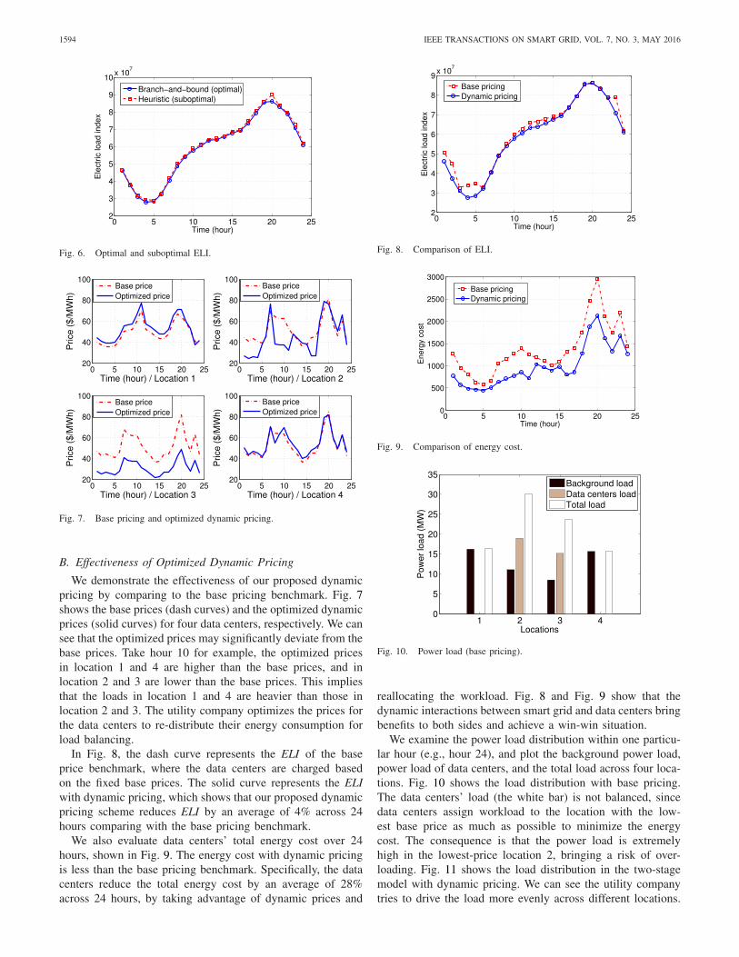
Fig. 6. Optimal and suboptimal ELI.

Fig. 7. Base pricing and optimized dynamic pricing.

B. Effectiveness of Optimized Dynamic Pricing

We demonstrate the effectiveness of our proposed dynamicpricing by comparing to the base pricing benchmark. Fig. 7shows the base prices (dash curves) and the optimized dynamicprices (solid curves) for four data centers, respectively. We cansee that the optimized prices may significantly deviate from thebase prices. Take hour 10 for example, the optimized pricesin location 1 and 4 are higher than the base prices, and inlocation 2 and 3 are lower than the base prices. This impliesthat the loads in location 1 and 4 are heavier than those inlocation 2 and 3. The utility company optimizes the prices forthe data centers to re-distribute their energy consumption forload balancing.

In Fig. 8, the dash curve represents the ELI of the baseprice benchmark, where the data centers are charged basedon the fixed base prices. The solid curve represents the ELIwith dynamic pricing, which shows that our proposed dynamicpricing scheme reduces ELI by an average of 4% across 24hours comparing with the base pricing benchmark.

We also evaluate data centers’ total energy cost over 24hours, shown in Fig. 9. The energy cost with dynamic pricingis less than the base pricing benchmark. Specifically, the datacenters reduce the total energy cost by an average of 28%across 24 hours, by taking advantage of dynamic prices and

Fig. 8. Comparison of ELI.

Fig. 9. Comparison of energy cost.

Fig. 10. Power load (base pricing).

reallocating the workload. Fig. 8 and Fig. 9 show that thedynamic interactions between smart grid and data centers bringbenefits to both sides and achieve a win-win situation.

We examine the power load distribution within one particu-lar hour (e.g., hour 24), and plot the background power load,power load of data centers, and the total load across four loca-tions. Fig. 10 shows the load distribution with base pricing.The data centers’ load (the white bar) is not balanced, sincedata centers assign workload to the location with the low-est base price as much as possible to minimize the energycost. The consequence is that the power load is extremelyhigh in the lowest-price location 2, bringing a risk of over-loading. Fig. 11 shows the load distribution in the two-stagemodel with dynamic pricing. We can see the utility companytries to drive the load more evenly across different locations.


Fig. 11. Power load (dynamic pricing).

Fig. 12. ELI performance with prediction error.

Therefore, our proposed scheme can effectively improve thereliability of smart grid through re-balancing power load acrossdifferent locations.

C. Impact of Prediction Errors

We conduct a case study to show the impact of predictionerrors on the ELI performance. We set the bounds (�t

i,minand �t

i,max) of the prediction errors as ±10% of the pre-dicted values Bt

i in location i and time slot t. Solving problemWCP in Section VI, we obtain the optimized worst-case ELIperformance as dash curve in Fig. 12. We also randomly gen-erate a realization of prediction errors, and compare the ELIperformance under the scenario with and without consideringthe prediction errors. If prediction errors are considered whenoptimizing the Stage-1 problem, the realized ELI performance(solid curve) can be guaranteed to be better than the worst-case ELI. However, if the prediction is assumed to be accuratewith zero error (while in reality it is not), then the ELI per-formance (dash curve) can be even worse than the worst-casebenchmark (e.g., in the 20th time slot). Therefore, the resultsdemonstrate the effectiveness of our proposed worst-case per-formance optimization problem, which provides a performanceguarantee for ELI under prediction errors.

VIII. CONCLUSION

In this paper, we studied the dynamic interactionsbetween smart grid and data centers as a two-stage priceoptimization problem. To solve the two-stage optimization

problem, we reformulated it as a mixed integer quadraticprogramming problem, and proposed a branch-and-boundalgorithm to attain the globally optimal solution, and a lowcomplexity heuristic descent algorithm to yield a close-to-optimal solution. The simulation results showed a win-winsolution for both the utility company and data centers.

For future work, we would like to study the interactionbetween the utility company and data centers with high pene-tration of renewable energy and under incomplete information.Some cloud provides installed renewable energy facilities topower data centers. How to manage the renewable-powereddata centers and what is the impact on the power systemare worthy of study. The utility company may not able toacquire private information of data-center operation, so howto incentivize data centers with asymmetric information is aninteresting and practical problem for future study.

REFERENCES

[1] H. Wang, J. Huang, X. Lin, and H. Mohsenian-Rad, “Exploring smartgrid and data center interactions for electric power load balancing,”in Proc. ACM Greenmetrics, Pittsburgh, PA, USA, Jun. 2013, pp. 1–6.

[2] A. Qureshi, R. Weber, H. Balakrishnan, J. Guttag, and B. Maggs,“Cutting the electric bill for Internet-scale systems,” in Proc. ACMSIGCOMM, Barcelona, Spain, 2009, pp. 123–134.

[3] M. Pedram, “Energy-efficient datacenters,” IEEE Trans. Comput.-AidedDesign Integr. Circuits Syst., vol. 31, no. 10, pp. 1465–1484, Oct. 2012.

[4] L. Rao, X. Liu, L. Xie, and W. Liu, “Minimizing electricity cost:Optimization of distributed Internet data centers in a multi-electricity-market environment,” in Proc. IEEE INFOCOM, San Diego, CA, USA,2010, pp. 1–9.

[5] Z. Liu, M. Lin, A. Wierman, S. H. Low, and L. L. H. Andrew, “Greeninggeographical load balancing,” in Proc. ACM SIGMETRICS, Portland,OR, USA, 2011, pp. 233–244.

[6] M. Lin, Z. Liu, A. Wierman, and L. L. H. Andrew, “Online algorithmsfor geographical load balancing,” in Proc. IEEE IGCC, San Jose, CA,USA, 2012, pp. 1–10.

[7] M. Ghamkhari and H. Mohsenian-Rad, “Energy and performance man-agement of green data centers: A profit maximization approach,” IEEETrans. Smart Grid, vol. 4, no. 2, pp. 1017–1025, Jun. 2013.

[8] P. Wang, L. Rao, X. Liu, and Y. Qi, “D-Pro: Dynamic data center oper-ations with demand-responsive electricity prices in smart grid,” IEEETrans. Smart Grid, vol. 3, no. 4, pp. 1743–1754, Dec. 2012.

[9] L. Zhang, S. Ren, C. Wu, and Z. Li, “A truthful incentive mechanismfor emergency demand response in colocation data centers,” in Proc.IEEE INFOCOM, Hong Kong, 2015, pp. 2632–2640.

[10] A.-H. Mohsenian-Rad and A. Leon-Garcia, “Energy-information trans-mission tradeoff in green cloud computing,” in Proc. IEEE Globecom,Miami, FL, USA, 2010, pp. 1–6.

[11] A.-H. Mohsenian-Rad and A. Leon-Garcia, “Coordination of cloudcomputing and smart power grids,” in Proc. IEEE SmartGridComm,Gaithersburg, MD, USA, 2010, pp. 368–372.

[12] X. Fang, S. Misra, G. Xue, and D. Yang, “Smart grid—The new andimproved power grid: A survey,” IEEE Commun. Surveys Tuts., vol. 14,no. 4, pp. 944–980, Dec. 2012.

[13] A.-H. Mohsenian-Rad and A. Leon-Garcia, “Optimal residential loadcontrol with price prediction in real-time electricity pricing environ-ments,” IEEE Trans. Smart Grid, vol. 1, no. 2, pp. 120–133, Sep. 2010.

[14] H. K. Nguyen, J. B. Song, and Z. Han, “Demand side management toreduce peak-to-average ratio using game theory in smart grid,” in Proc.IEEE INFOCOM Workshops, Orlando, FL, USA, 2012, pp. 91–96.

[15] N. Li, L. Chen, and S.H. Low, “Optimal demand response based on util-ity maximization in power networks,” in Proc. IEEE PES Gen. Meeting,San Diego, CA, USA, 2011, pp. 1–8.

[16] C. Joe-Wong, S. Ha, S. Sen, and M. Chiang, “Optimized day-aheadpricing for smart grid with device-specific scheduling flexibility,” IEEEJ. Sel. Areas Commun., vol. 30, no. 6, pp. 1075–1085, Jul. 2012.

[17] N. H. Tran et al., “How geo-distributed data centers do demandresponse: A game-theoretic approach,” IEEE Trans. Smart Grid,Doi: 10.1109/TSG.2015.2421286.


[18] (Aug. 2015). Data Center Map. [Online]. Available:http://www.datacentermap.com/usa/california/

[19] H. Xu and B. Li, “Reducing electricity demand charge for data centerswith partial execution,” in Proc. ACM e-Energy, Cambridge, U.K., 2014,pp. 51–61.

[20] J. Lai et al., “Evaluation of evolving residential electricity tariffs,” Dept.Environ. Energy, Ernest Orlando Lawrence Berkeley Nat. Lab., Berkeley,CA, USA, Tech. Rep. LBNL-4496E, 2011.

[21] L. A. Barroso and U. Holzle, “The case for energy-proportionalcomputing,” Computer, vol. 40, no. 12, pp. 33–37, Dec. 2007.

[22] A. Qureshi, “Power-demand routing in massive geo-distributed sys-tems,” Ph.D. dissertation, Dept. Comput. Sci. Eng., Mass. Inst. Technol.,Cambridge, MA, USA, 2010.

[23] A. Motamedi, H. Zareipour, and W. D. Rosehart, “Electricity price anddemand forecasting in smart grids,” IEEE Trans. Smart Grid, vol. 3,no. 2, pp. 664–674, Jun. 2012.

[24] M. Zugno, J. M. Morales, P. Pinson, and H. Madsen, “A bilevel modelfor electricity retailers’ participation in a demand response marketenvironment,” Energy Econ., vol. 36, pp. 182–197, Mar. 2013.

[25] S. P. Boyd and L. Vandenberghe, Convex Optimization. Cambridge,U.K.: Cambridge Univ. Press, 2004.

[26] Y. Yuan, Z. Li, and K. Ren, “Quantitative analysis of load redistributionattacks in power systems,” IEEE Trans. Parallel Distrib. Syst., vol. 23,no. 9, pp. 1731–1738, Sep. 2012.

[27] J. F. Bard, Practical Bilevel Optimization: Algorithms and Applications.Boston, MA, USA: Kluwer Academic, 1998.

[28] A. Ben-tal and A. Nemirovski, “Selected topics in robust convexoptimization,” Math. Program., vol. 112, no. 1, pp. 125–158, 2008.

[29] (Mar. 2013). Market Data. [Online]. Available: http://www.iso-ne.com[30] (Mar. 2013). Market Data. [Online]. Available: http://www.nyiso.com[31] (Apr. 2015). Google Traffic Disruptions. [Online]. Available:

http://www.google.com/transparencyreport/traffic/data/[32] Z. Sun, F. Kong, X. Liu, X. Zhou, and X. Chen, “Intelligent joint spatio-

temporal management of electric vehicle charging and data center powerconsumption,” in Proc. IGCC, Dallas, TX, USA, 2014, pp. 1–8.

[33] H. Wang, J. Huang, X. Lin, and H. Mohsenian-Rad. (Nov. 2, 2015).Proactive Demand Response for Data Centers: A Win-Win Solution.[Online]. Available: http://arxiv.org/abs/1511.00575

Hao Wang (S’10) is currently pursuing thePh.D. degree with the Department of InformationEngineering, Chinese University of Hong Kong. Hisresearch interests are in the control and optimizationof network systems with a recent focus on the bigdata analytics of renewable energy, operations, andeconomics of smart grid.

Jianwei Huang (S’01–M’06–SM’11) received thePh.D. degree from Northwestern University in 2005.He is an Associate Professor, and a Directorof the Network Communications and EconomicsLaboratory, Department of Information Engineering,Chinese University of Hong Kong. He worked asa Postdoctoral Research Associate in Princeton,from 2005 to 2007. He has co-authored fourbooks entitled Wireless Network Pricing, MonotonicOptimization in Communication and NetworkingSystems, Cognitive Mobile Virtual Network Operator

Games, and Social Cognitive Radio Networks. He was a co-recipient of eightinternational best paper awards, including the IEEE Marconi Prize PaperAward in Wireless Communications in 2011. He has served as an Editor forseveral top IEEE Communications journals, including the IEEE JOURNAL

ON SELECTED AREAS IN COMMUNICATIONS, TWC, and TCCN, and a TPCChair of many international conferences. He is the Vice Chair of the IEEEComSoc Cognitive Network Technical Committee and the Past Chair of theIEEE ComSoc Multimedia Communications Technical Committee. He is aDistinguished Lecturer of the IEEE Communications Society.

Xiaojun Lin (S’02–M’05–SM’12) received theB.S. degree from Zhongshan University, Guangzhou,China, in 1994, and the M.S. and Ph.D. degrees fromPurdue University, West Lafayette, Indiana, in 2000and 2005, respectively. He is currently an AssociateProfessor of Electrical and Computer Engineeringwith Purdue University. His current research inter-ests are in the analysis, control, and optimizationof large communication networks and cyber-physicalsystems.

Dr. Lin was a recipient of the IEEE INFOCOM2008 Best Paper Award and the 2005 Best Paper of the Year Award from theJournal of Communications and Networks, and the NSF CAREER awardin 2007. His paper was also one of two runner-up papers for the Best-Paper award at IEEE INFOCOM 2005. He was the Workshop Co-Chairfor IEEE GLOBECOM 2007, the Panel Co-Chair for WICON 2008, theTPC Co-Chair for ACM MobiHoc 2009, and the Mini-Conference Co-Chairfor IEEE INFOCOM 2012. He is currently serving as an Associate Editorfor the IEEE/ACM TRANSACTIONS ON NETWORKING, an Area Editor forComputer Networks, and has served as a Guest Editor for Ad Hoc Networks.

Hamed Mohsenian-Rad (S’04–M’09–SM’14)received the Ph.D. degree in electrical and com-puter engineering from the University of BritishColumbia, Vancouver, Canada, in 2008. He iscurrently an Assistant Professor of ElectricalEngineering with the University of California atRiverside. His research interests include modeling,analysis, and optimization of power systems andsmart grids with focus on energy storage, renewablepower generation, demand response, cyber-physicalsecurity, and large-scale power data analysis. He

was a recipient of the National Science Foundation CAREER Award in 2012,the Best Paper Award from the IEEE Power and Energy Society GeneralMeeting in 2013, and the Best Paper Award from the IEEE InternationalConference on Smart Grid Communications in 2012. He serves as anEditor for the IEEE TRANSACTIONS ON SMART GRID, IEEE POWER

ENGINEERING LETTERS, and IEEE COMMUNICATIONS LETTERS.

1584 ieee transactions on smart grid, vol. 7, no. 3, may

Documents