1

Monte Carlo Rendering

Last Time?• Modern Graphics Hardware• Cg Programming Language• Gouraud Shading vs.

Phong Normal Interpolation• Bump, Displacement, & Environment Mapping• Cg Examples

GP

R

T

FP

D

Today• Does Ray Tracing Simulate Physics?• Monte-Carlo Integration• Sampling• Advanced Monte-Carlo Rendering

Does Ray Tracing Simulate Physics?• No…. traditional ray tracing is also called

“backward” ray tracing• In reality, photons actually travel from the light

to the eye

Forward Ray Tracing• Start from the light source

– But very, very low probability to reach the eye• What can we do about it?

– Always send a ray to the eye…. still not efficient

Transparent Shadows?• What to do if the shadow ray sent to the light source

intersects a transparent object?– Pretend it’s opaque?– Multiply by transparency color?

(ignores refraction & does not produce caustics)

• Unfortunately, ray tracing is full of dirty tricks

2

Is this Traditional Ray Tracing?

• No, Refraction and complex reflection for illumination are not handled properly in traditional (backward) ray tracing

Images by Henrik Wann Jensen

Refraction and the Lifeguard Problem

• Running is faster than swimming Beach

Person in trouble

LifeguardWater

Run

Swim

What makes a Rainbow?• Refraction is wavelength-dependent

– Refraction increases as the wavelength of light decreases– violet and blue experience more bending than orange and red

• Usually ignored in graphics • Rainbow is caused by

refraction + internal reflection + refraction

From “Color and Light in Nature”by Lynch and Livingstone

Pink Floyd, The Dark Side of the Moon

The Rendering Equation• Clean mathematical framework for light-

transport simulation• At each point, outgoing light in one direction

is the integral of incoming light in all directionsmultiplied by reflectance property

Today• Does Ray Tracing Simulate Physics?• Monte-Carlo Integration

– Probabilities and Variance– Analysis of Monte-Carlo Integration

• Sampling• Advanced Monte-Carlo Rendering

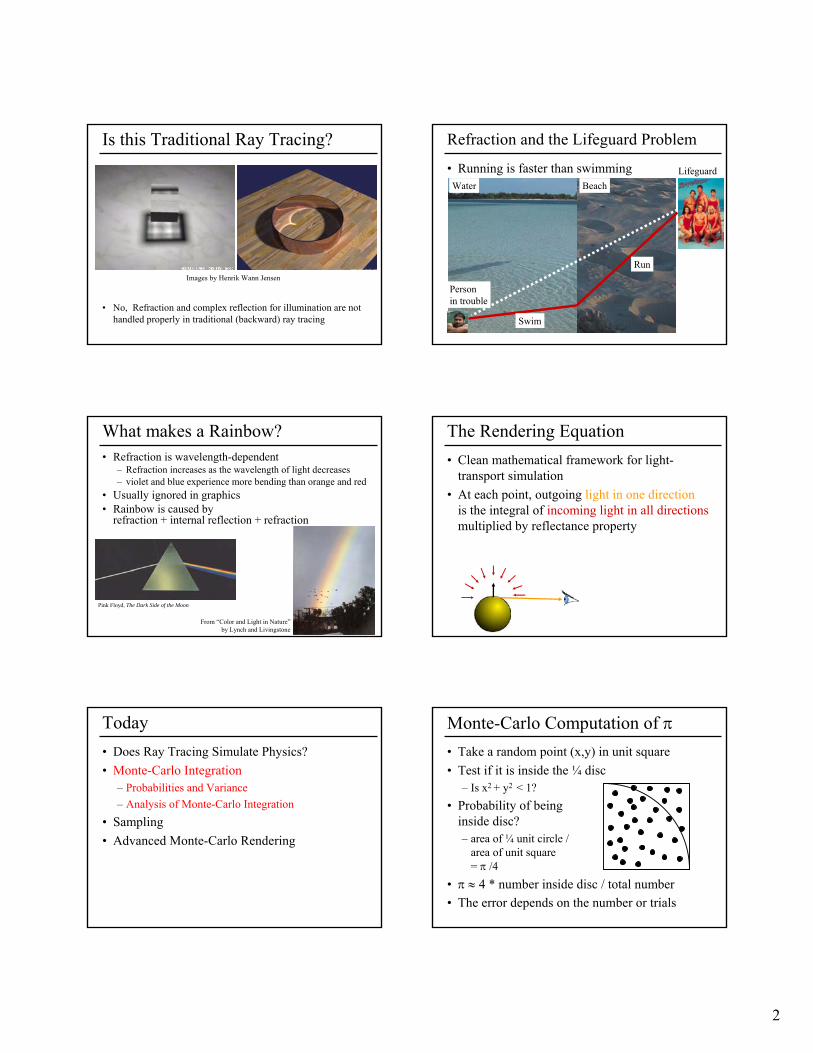
Monte-Carlo Computation of π• Take a random point (x,y) in unit square• Test if it is inside the ¼ disc

– Is x2 + y2 < 1?• Probability of being

inside disc? – area of ¼ unit circle /

area of unit square= π /4

• π ≈ 4 * number inside disc / total number• The error depends on the number or trials

3

Convergence & Error• Let’s compute 0.5 by flipping a coin:

– 1 flip: 0 or 1 → average error = 0.5

– 2 flips: 0, 0.5, 0.5 or 1 → average error = 0. 25

– 4 flips: 0 (*1),0.25 (*4), 0.5 (*6), 0.75(*4), 1(*1) → average error = 0.1875

• Unfortunately, doubling the number of samples does not double accuracy

Another Example:

• We know it should be 1.0

• In practicewith uniform samples:

N

σ2

- σ2

error

Review of (Discrete) Probability• Random variable can take discrete values xi

• Probability pi for each xi

0 < pi < 1, Σ pi =1• Expected value

• Expected value of function of random variable– f(xi) is also a random variable

Variance & Standard Deviation• Variance σ 2: deviation from expected value• Expected value of square difference

• Also

• Standard deviation σ: square root of variance (notion of error, RMS)

Monte Carlo Integration• Turn integral into finite sum• Use n random samples• As n increases…

– Expected value remains the same– Variance decreases by n– Standard deviation (error) decreases by

• Thus, converges with

n1

n1

Advantages of MC Integration• Few restrictions on the integrand

– Doesn’t need to be continuous, smooth, ...– Only need to be able to evaluate at a point

• Extends to high-dimensional problems– Same convergence

• Conceptually straightforward• Efficient for solving at just a few points

4

Disadvantages of MC Integration• Noisy• Slow convergence • Good implementation is hard

– Debugging code– Debugging math– Choosing appropriate techniques

• Punctual technique, no notion of smoothness of function (e.g., between neighboring pixels)

Questions?

256 glossy samples per pixel

1 glossy sample per pixel

Today• Does Ray Tracing Simulate Physics?• Monte-Carlo Integration• Sampling

– Stratified Sampling– Importance Sampling

• Advanced Monte-Carlo Rendering

Domains of Integration• Pixel, lens (Euclidean 2D domain)• Time (1D)• Hemisphere

– Work needed to ensure uniform probability

Example: Light Source• We can integrate over surface or over angle• But we must be careful to get probabilities and

integration measure right!

source

hemisphere

Sampling the source uniformly Sampling the hemisphere uniformly

Stratified Sampling• With uniform sampling, we can get unlucky

– E.g. all samples in a corner

• To prevent it, subdivide domain Ωinto non-overlapping regions Ωi– Each region is called a stratum

• Take one random samples per Ωi

5

Example• Borrowed from Henrik Wann Jensen

Unstratified Stratified

Glossy Rendering• Integrate over hemisphere• BRDF times cosine times incoming light

)( iωI

Slide from Jason Lawrence

Sampling a BRDF

5 Samples/Pixel

oω)(U iω

)(P iωoω

Slide from Jason Lawrence

Sampling a BRDF

25 Samples/Pixel

)(U iωoω

)(P iωoω

Slide from Jason Lawrence

Sampling a BRDF

75 Samples/Pixel

)(U iωoω

)(P iωoω

Slide from Jason Lawrence

uniformbad good

Importance Sampling

• Choose p wisely to reduce variance– p that resembles f– Does not change convergence rate (still sqrt)– But decreases the constant

6

Results

Traditional importance functionTraditional importance function Better importance by Lawrence et al. Better importance by Lawrence et al.

1200 Samples/Pixel

Today• Does Ray Tracing Simulate Physics?• Monte-Carlo Integration• Sampling• Advanced Monte-Carlo Rendering

Ray Casting• Cast a ray from the eye through each pixel

Ray Tracing• Cast a ray from the eye through each pixel • Trace secondary rays (light, reflection, refraction)

Monte-Carlo Ray Tracing• Cast a ray from the eye through each pixel• Cast random rays to accumulate radiance contribution

– Recurse to solve the Rendering Equation

Should also systematically

sample the primary light

Importance of Sampling the LightWithout explicit

light samplingWith explicit light sampling

1 path per pixel

4 path per pixel

7

Monte Carlo Path Tracing• Trace only one secondary ray per recursion• But send many primary rays per pixel

(performs antialiasing as well)

Ray Tracing vs Path Tracing2 bounces5 glossy samples 5 shadow samples

How many rays cast per pixel?

1main ray + 5 shadow rays +5 glossy rays + 5x5 shadow rays +5*5 glossy rays + 5x5x5 shadow rays = 186 rays

How many 3 bounce paths can we trace per pixel for the same cost?

186 rays / 8 ray casts per path = ~23 paths

Which will probably have less error?

Results: 10 paths/pixel Results: 100 paths/pixel

Reading for Today

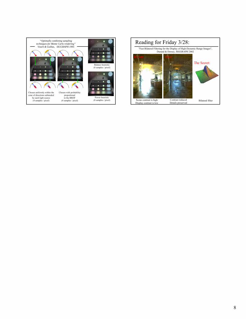
Naïve sampling strategy Optimal sampling strategy

Veach & Guibas "Optimally Combining Sampling Techniques

for Monte Carlo Rendering" SIGGRAPH 95

Sampling

uniform sampling(or uniform random)

dense sampling where function has greater magnitude

all samples weighted equally

weights (width) for dense samples are reduced

To optimally combine samples from different

distributions,weight more highly the

samples from the locally densest

distribution

sensitive to choice of samples

less sensitive to choice of

samples

8

Chosen uniformly within the cone of directions subtended

by each light source(4 samples / pixel)

Chosen with probability proportional to the BRDF

(4 samples / pixel)

“Optimally combining sampling techniques for Monte Carlo rendering”

Veach & Guibas, SIGGRAPH 1995

Power heuristic(8 samples / pixel)

Balance heuristic(8 samples / pixel)

Reading for Friday 3/28:"Fast Bilateral Filtering for the Display of High-Dynamic Range Images",

Durand & Dorsey, SIGGRAPH 2002

Scene contrast is highDisplay contrast is low

Contrast reducedDetails preserved

Before After

The Secret:

Bilateral filter