18.330 spring 2012 introduction to numerical analysis...
TRANSCRIPT

18.330 Spring 2012Introduction to numerical analysis
Class notes
Laurent DemanetDraft April 25, 2014

2

Preface
Good additional references are
• Burden and Faires, Introduction to numerical analysis
• Suli and Mayers, Introduction to numerical analysis
• Trefethen, Spectral methods in Matlab
as well as the pdf notes on numerical analysis by John Neu.If the text points you to some external reference for further study, the
latter is obviously not part of the material for the class.We will very likely skip several sections in chapters 7 and 8 for 18.330.Work in progress!
3

4

Chapter 1
Series and sequences
Throughout these notes we’ll keep running into Taylor series and Fourier se-ries. It’s important to understand what is meant by convergence of series be-fore getting to numerical analysis proper. These notes are sef-contained, buttwo good extra references for this chapter are Tao, Analysis I; and Dahlquistand Bjorck, Numerical methods.
A sequence is a possibly infinite collection of numbers lined up in someorder:
a1, a2, a3, . . .
A series is a possibly infinite sum:
a1 + a2 + a3 + . . .
We’ll consider real numbers for the time being, but the generalization tocomplex numbers is a nice exercise which mostly consists in replacing eachoccurrence of an absolute value by a modulus.
The questions we address in this chapter are:
• What is the meaning of an infinite sum?
• Is this meaning ever ambiguous?
• How can we show convergence vs. divergence?
• When can we use the usual rules for finite sums in the infinite case?
5

6 CHAPTER 1. SERIES AND SEQUENCES
1.1 Convergence vs. divergence
We view infinite sums as limits of partial sums. Since partial sums aresequences, let us first review convergence of sequences.
Definition 1. A sequence (aj)∞j=0 is said to be ε-close to a number b if there
exists a number N ≥ 0 (it can be very large), such that for all n ≥ N ,
|aj − b| ≤ ε.
A sequence (aj)∞j=0 is said to converge to b if it is ε-close to b for all ε > 0
(however small). We then write aj → b, or limj→∞ aj = b.
If a sequence does not converge we say that it diverges. Unboundedsequences, i.e., sequences that contain arbitrarily large numbers, always di-verge. (So we never say “converges to infinity”, although it’s fine to say“diverges to infinity”.)
Examples:
• e−n → 0 as n→∞, and convergence is very fast.
• n/(n+ 2)→ 1 as n→∞, and convergence is rather slow.
• (−1)n is bounded, but does not converge.
• log(n) → ∞ as n → ∞, so the sequence diverges. For a proof thatlog(n) takes on arbitrarily large values, fix any large integer m. Doesthere exist an n such that log(n) ≥ m? Yes, it suffices to take n ≥ em.
Definition 2. Consider a sequence (aj)∞j=0. We define the N-th partial sum
SN as
SN = a0 + a1 + . . .+ aN =N∑j=0
aj.
We say that the series∑
j aj converges if the sequence of partial sums SNconverges to some number b as N →∞. We then write
∑∞j=0 aj = b.
Again, if a series does not converge we say that it diverges.

1.1. CONVERGENCE VS. DIVERGENCE 7
Example 1. Consider∑∞
j=0 2−j, i.e.,
1 +1
2+
1
4+
1
8+ . . . .
This series converges to the limit 2. To prove this, consider the partial sum
SN =N∑j=0
2−j.
Let us show by induction that SN = 2 − 2−N . The base case N = 0 is truesince 2−0 = 2−2−0. For the induction case, assume SN = 2−2−N . We thenwrite
SN+1 = SN + 2−(N+1) = (2− 2−N) + 2−(N+1) = 2− 2−(N+1),
the desired conclusion.
Example 2. The previous example was the x = 1/2 special case of the so-called geometric series
1 + x+ x2 + x3 + . . .
WIth a similar argument, we obtain the limit as
∞∑j=0
xj =1
1− x,
provided the condition |x| < 1 holds. This expression can also be seen as theTaylor expansion of 1/(1−x), centered at zero, and with radius of convergence1.
Example 3. Consider the so-called harmonic series
1 +1
2+
1
3+
1
4+ . . . .
This series diverges. To see this, let us show that the N partial sum iscomparable to log(N). We use the integral test
SN =N∑j=1
1
j≥∫ N+1
1
1
xdx.
(Insert picture here)The latter integral is log(N+1), which diverges as a sequence. The partial
sums, which are larger, must therefore also diverge.

8 CHAPTER 1. SERIES AND SEQUENCES
Example 4. Consider∞∑j=1
1
nq,
for some q > 0. As a function of q, this is the Riemann zeta function ζ(q).(A fascinating object for number theorists.)
We’ve seen above that q = 1 leads to divergence. A similar integral testwould show that the series converges when q > 1, while it diverges whenq ≤ 1.
We now switch to a finer understanding of convergence: certain series areabsolutely convergent, while others are conditionally convergent. This willaffect what type of algebraic manipulations can be done on them.
Definition 3. A series∑∞
j=0 aj is said to be absolutely convergent if∑∞
j=0 |aj|converges. If a series is not absolutely convergent, but nevertheless converges,we say that it is conditionally convergent.
The subtlety with conditional convergence is that alternating plus andminus signs may lead to convergence because of cancelations when summingconsecutive terms.
Example 5. Consider
1− 1
2+
1
3− 1
4+
1
5− 1
6+ . . . .
This series is not absolutely convergent, because it reduces to the harmonicseries when absolute values of the terms are taken. It is nevertheless con-vergent, hence conditionally convergent, as the following argument shows.Assume N is even, and let
SN =N∑j=1
(−1)j
j.
Terms can be grouped 2-by-2 to obtain, for j ≥ 1,
1
j− 1
j + 1=
1
j(j + 1).

1.1. CONVERGENCE VS. DIVERGENCE 9
A fortiori, 1j(j+1)
≤ 1j2
, so
SN ≤N−1∑
j=1,3,5,...
1
j2,
which we know converges. If on the other hand N is odd, then SN = SN−1 +1
N+1. Both terms SN and 1/(N + 1) are converging sequences, so their sum
converges as well. This proves convergence.Note that the series converges to
1− 1
2+
1
3− 1
4+
1
5− 1
6+ . . . = log(2).
This is the special case x = 1 in the Taylor expansion of log(1 + x) aboutx = 0.
In passing, without proof, here is a useful test to check convergence ofalternating series.
Theorem 1. (Alternating series test) Consider the series
∞∑j=0
(−1)jaj,
where aj > 0. If (aj) converges to zero (as a sequence), then the series isconvergent.
The main problem with conditionally convergent series is that if the termsare rearranged, then the series may converge to a different limit. The “safezone” for handling infinite sums as if they were finite is when convergence isabsolute.
Theorem 2. Let f : Z+ 7→ Z+ be a bijection, i.e., f is a rearrangement of thenonnegative integers. Consider a series
∑∞j=0 aj. If this series is absolutely
convergent, then∞∑j=0
aj =∞∑j=0
af(j).
Here is what usually happens when the assumption of absolute conver-gence is not satisfied.

10 CHAPTER 1. SERIES AND SEQUENCES
Example 6. Consider again
1
3− 1
4+
1
5− 1
6+ . . .
which as we have seen equals log(2)− (1− 1/2) = log(2)− 1/2 = .193147 . . ..We can rearrange the terms of the series by assigning two negative terms foreach positive term:
1
3− 1
4− 1
6+
1
5− 1
8− 1
10+
1
7+ . . .
This series is also convergent, but happens to converge to (log(2) − 1)/2 =−.153426 . . ..
Other operations that can be safely performed on absolutely convergentseries are passing absolute values inside the sum, and exchanging sums.Again, complications arise if the series is only conditionally convergent. (SeeTao, Analysis I, for counter-examples.)
Theorem 3. The following operations are legitimate for absolutely conver-gent series.
• Passing absolute values inside sums:
|∞∑j=0
aj| ≤∞∑j=0
|aj|.
• Swapping sums:∞∑j=0
∞∑k=0
aj,k =∞∑k=0
∞∑j=0
aj,k
Note in passing that the same is true for integrals of unbounded integrandsor integrals over unbounded domains: they need to be absolutely convergent(integrability of the absolute value of the function) for the integral swap to belegitimate. This is the content of Fubini’s theorem. Again, there are strikingcounter-examples when the integrals are not absolutely convergent and theswap doesn’t work (See Tao, Analysis I).

1.2. THE BIG-O NOTATION 11
1.2 The big-O notation
Here are a few useful pieces of notation for comparing growth or decay ofsequences, used extensively by numerical analysts. They are called the big-O, little-o, and big-Theta notations. Big-O is used much more often thanthe other two. They occur when comparing decay rates of truncation errors,and runtimes of algorithms.
Definition 4. Consider two nonzero sequences fn and gn for n = 0, 1, 2, . . ..We write fn = O(gn) when there exists C > 0 such that |fn| ≤ C|gn|.We write fn = o(gn) when fn/gn → 0 as n→∞.We write fn = Θ(gn) when fn = O(gn) and gn = O(fn).
Examples:
• fn = n2 and gn = n3: we have n2 = O(n3) and n2 = o(n3) butn2 6= Θ(n3).
• fn = nn+2
and gn = nn−3 : we have fn = O(gn) and fn = Θ(gn), but
fn 6= o(gn).
• Exponentials always dominate polynomials: na = o(ebn) whatever a >0 and b > 0.
• Conversely, e−bn = o(n−a).
Out loud, we can read the expression fn = O(gn) as “fn in on the orderof gn”.
The same notations can be used to compare sequences indexed by a pa-rameter that goes to zero, such as (typically) the grid spacing h. The defini-tion above is simply adapted by letting h→ 0 rather than n→∞.
Examples:
• f(h) = h2 and g(h) = h3: this time we have g(h) = O(f(h)) andg(h) = o(f(h)) when the limit of interest is h→ 0.
• Powers of h don’t converge to zero nearly as fast as this exponential:ea/h = o(hb) whatever a > 0 and b > 0.
SImilarly, we may wish to compare functions f and g of a continuousvariable x as either x→∞ or x→ 0; the definition is again modified in theobvious way. Whenever a O(·) or o(·) is written, some underlying limit isunderstood.

12 CHAPTER 1. SERIES AND SEQUENCES

Chapter 2
Integrals as sums andderivatives as differences
We now switch to the simplest methods for integrating or differentiating afunction from its function samples. A careful study of Taylor expansionsreveals how accurate the constructions are.
2.1 Numerical integration
Consider a function f – we’ll specify which assumptions we need to makeabout it in a minute. Let us reformulate the integral∫ 1
0
f(x) dx
by breaking up the interval [a, b] into subintervals [xj−1, xj], with xj = jh,h = 1/N , and
0 = x0 < x1 < . . . < xN = 1.
Together, the (xj) are called a Cartesian grid. Still without approximation,we can write ∫ 1
0
f(x) dx =N∑j=1
∫ xj
xj−1
f(x) dx.
A quadrature is obtained when integrals are approximated by quantities thatdepend only on the samples f(xj) of f on the grid xj. For instance, we can
13

14CHAPTER 2. INTEGRALS AS SUMS ANDDERIVATIVES AS DIFFERENCES
approximate the integral over [xj−1, xj] by the signed area of the rectangleof height f(xj−1) and width h:∫ xj
xj−1
f(x) dx ' hf(xj−1).
Putting the terms back together, we obtain the rectangle method :∫ 1
0
f(x) dx ' hN∑j=1
f(xj−1).
(Insert picture here)To understand the accuracy of this approximation, we need a detour
through Taylor expansions. Given a very smooth function f(x), it sometimesmakes sense to write an expansion around the point x = a, as
f(x) = f(a) + f ′(a)(x− a) +1
2f ′′(a)(x− a)2 +
1
3!f ′′′(a)(x− a)3 + . . .
As a compact series, this would be written as
f(x) =∞∑n=0
1
n!f (n)(a)(x− a)n,
where n! = n · (n− 1) · . . . 2 · 1 is the factorial of n. The word “sometimes” isimportant: the formula above requires the function to be infinitely differen-tiable, and even still, we would need to make sure that the series converges(by means of the analysis of the previous chapter). The radius of conver-gence of the Taylor expansion is the largest R such that, for all x such that|x− a| < R, the series converges.
It is also possible to truncate a Taylor series after N terms, as
f(x) =N−1∑n=0
1
n!f (n)(a)(x− a)n +
1
N !f (N)(y)(x− a)N , (2.1)
where y is some number between x and a. The formula does not specify whatthe number y is; only that there exists one such that the remainder takesthe form of the last term. In spite of the fact that y is unspecified, this is amuch more useful form of Taylor expansion than the infinite series:

2.1. NUMERICAL INTEGRATION 15
• We often only care about the size of the remainder, and write inequal-ities such as
| 1
N !f (N)(y)(x− a)N | ≤ 1
N !
(maxz∈[x,a]
|f (N)(z)|)|x− a|N ,
or, for short,1
N !f (N)(y)(x− a)N = O(|x− a|N),
where all the “constants” are hidden in the O. So, the remainder ison the order of |x − a|N . The limit implicit in the O notation is herex− a→ 0.
• The finite-N formula is valid whenever the function is N times differ-entiable, not infinitely differentiable! In fact, the Taylor series itselfmay diverge, but equation (2.1) is still valid.
In order to study the problem of approximating∫ xjxj−1
f(x) dx, let us ex-
pand f in a (short, truncated) Taylor series near x = xj−1:
f(x) = f(xj−1) + f ′(y(x))h,
where y(x) ∈ [xj−1, x]. We’ve written y(x) to highlight that it depends onx. This works as long as f has one derivative. Integrating on both sides,and recognizing that f(xj−1) is constant with respect to x, we get (recallxj − xj−1 = h) ∫ xj
xj−1
f(x) dx = hf(xj−1) + h
∫ xj
xj−1
f ′(y(x)) dx.
We don’t know much about y(x), but we can certainly write the inequality
h |∫ xj
xj−1
f ′(y(x)) dx| ≤ h maxy∈[xj−1,xj ]
|f ′(y)|∫ xj
xj−1
1 dx = h2 maxy∈[xj−1,xj ]
|f ′(y)|.
So, as long as f is differentiable, we have∫ xj
xj−1
f(x) dx = hf(xj−1) +O(h2),

16CHAPTER 2. INTEGRALS AS SUMS ANDDERIVATIVES AS DIFFERENCES
where the derivative of f hides in the O sign. The integral over [0, 1] has Nsuch terms, so when they are added up the error compounds to N ·O(h2) =O(h) (because h = 1/N). Thus we have just proved that∫ 1
0
f(x) dx ' h
N∑j=1
f(xj−1) +O(h).
The error is on the order of the grid spacing h itself, so we say the methodis first-order accurate (because the exponent of h is one.)
Choosing the (signed) height of each rectangle from the left endpoint xj−1does not sound like the most accurate thing to do. Evaluating the functioninstead at xj−1/2 = (j − 1/2)h is a better idea, called the midpoint method.It is possible to show that∫ 1
0
f(x) dx ' hN∑j=1
f(xj−1/2) +O(h2),
provided the function f is twice differentiable (because f ′′ hides in the Osign). The accuracy is improved, since h2 gets much smaller than h as h→ 0.We say the midpoint method is second-order accurate.
Another solution to getting order-2 accuracy is to consider trapezoidsinstead of rectangles for the interval [xj−1, xj]. The area of the trapezoidspanned by the 4 points (xj−1, 0); (xj−1, f(xj−1)); (xj, f(xj)); (xj, 0) is h(f(xj−1)+f(xj))/2. This gives rise to the so-called trapezoidal method, or trapezoidalrule.
(Insert picture here)Let us compare this quantity to the integral of f over the same interval.
Consider the truncated Taylor expansions
f(x) = f(xj−1) + f ′(xj−1)(x− xj−1) +O(h2),
f(xj) = f(xj−1) + f ′(xj−1)h+O(h2),
where the second derivative of f appears in the O sign. Integrating the firstrelation gives ∫ xj
xj−1
f(x) dx = hf(xj−1) +h2
2f ′(xj−1) +O(h3).

2.1. NUMERICAL INTEGRATION 17
The area of the trapezoid, on the other hand, is (using the second Taylorrelation)
h
2(f(xj−1) + f(xj)) = hf(xj−1) +
h2
2f ′(xj−1) +O(h3).
Those two equations agree, except for the terms O(h3) which usually differin the two expressions. Hence∫ xj
xj−1
f(x) dx =h
2(f(xj−1) + f(xj)) +O(h3).
We can now sum over j (notice that all the terms appear twice, exceptfor the endpoints) to obtain∫ 1
0
f(x) dx =h
2f(0) + h
N−1∑j=1
f(xj) +h
2f(1) +O(h2).
The trapezoidal rule is second-order accurate. All it took is a modificationof the end terms to obtain O(h2) accuracy in place of O(h).
Example: f(x) = x2 in [0, 1]. We have∫ 1
0x2 dx = 1/3.
• For the rectangle rule with N = 4 and h = 1/4, consider the gridpointsx = 0, 1/4, 1/2, 3/4, and 1. Each rectangle has height f(xj−1) wherexj−1 is the left endpoint. We have∫ 1
0
x2 dx ' 1
4
[0 +
1
42+
1
22+
32
42
]=
14
64= .2188...
This is quite far (O(h), as we know) from 1/3.
• For the trapezoidal rule, consider the same grid. We now also considerthe grid point at x = 1, but the contribution of both x = 0 and x = 1is halved.∫ 1
0
x2 dx =1
4
[1
2· 0 +
1
42+
1
22+
32
42+
1
2· 1]
=22
64= .3438...
This is much closer (O(h2) as a matter of fact) from 1/3.
We’ll return to the topic of numerical integration later, after we coverpolynomial interpolation.

18CHAPTER 2. INTEGRALS AS SUMS ANDDERIVATIVES AS DIFFERENCES
2.2 Numerical differentiation
The simplest idea for computing an approximation to the derivative u′(xj)of a function u from the samples uj = u(xj) is to form finite difference ratios.On an equispaced grid xj = jh, the natural candidates are:
• the one-sided, forward and backward differences
∆+uj =uj+1 − uj
h, ∆− =
uj − uj−1h
,
• and the two-sided centered difference
∆0uj =uj+1 − uj−1
2h.
Let us justify the accuracy of these difference quotients at approximatingderivatives, as h → 0. The analysis will depend on the smoothness of theunderlying function u.
Assume without loss of generality that xj−1 = −h, xj = 0, and xj+1 = h.For the forward difference, we can use a Taylor expansion about zero to get
u(h) = u(0) + hu′(0) +h2
2u′′(ξ), ξ ∈ [0, h].
(The greek letter ξ is “xi”.) When substituted in the formula for the forwarddifference, we get
u(h)− u(0)
h= u′(0) +
h
2u′′(ξ).
The error is a O(h) as soon as the function has two bounded derivatives. Wesay that the forward difference is a method of order one. The analysis forthe backward difference is very similar.
For the centered difference, we now use two Taylor expansions about zero,for u(h) and u(−h), that we write up to order 3:
u(±h) = u(0)± hu′(0) +h2
2u′′(0)± h3
6u′′′(ξ),
with ξ either in [0, h] or [−h, 0] depending on the choice of sign. Subtractu(−h) from u(h) to get (the h2 terms cancel out)
u(h)− u(−h)
2h= u′(0) +
h2
3u′′′(ξ).

2.2. NUMERICAL DIFFERENTIATION 19
The error is now O(h2) provided u is three times differentiable, hence themethod is of order 2.
The simplest choice for the second derivative is the centered second dif-ference
∆2uj =uj+1 − 2uj + uj−1
h2.
It turns out that ∆2 = ∆+∆− = ∆−∆+, i.e., the three-point formula for thesecond difference can be obtained by calculating the forward difference of thebackward difference, or vice-versa. ∆2 is second-order accurate: the error isO(h2). To see this, write the Taylor expansions around x = 0 to fourth order:
u(±h) = u(0)± hu′(0) +h2
2u′′(0)± h3
6u′′′(0) +
h4
24u′′′′(ξ).
with ξ either in [0, h] or [−h, 0] depending on the choice of sign. The oddterms all cancel out when calculating the second difference, and what is leftis
uj+1 − 2uj + uj−1h2
= u′′(0) +h2
12u′′′′(ξ).
So the method really is O(h2) only when u is four times differentiable.Example: f(x) = x2 again. We get f ′(x) = 2x and f ′′(x) = 2.
∆+f(x) =(x+ h)2 − x2
h=
2xh+ h2
h= 2x+ h.
∆−f(x) =x2 − (x− h)2
h=
2xh− h2
h= 2x− h.
∆0f(x) =(x+ h)2 − (x− h)2
2h=
4xh
2h= 2x.
∆2f(x) =(x+ h)2 − 2x2 + (x− h)2
h2=
2h2
h2= 2.
The error is manifestly h for the forward difference, and −h for the backwarddifference (both are O(h).) Coincidentally, the error is zero for ∆0 and ∆2:centered differences differentiate parabolas exactly. This is an exception:finite differences are never exact in general. Of course, 0 = O(h2) so there’sno contradiction.
When u has less differentiability than is required by the remainder in theTaylor expansions, it may happen that the difference schemes may have lower

20CHAPTER 2. INTEGRALS AS SUMS ANDDERIVATIVES AS DIFFERENCES
order than advertised. This happens in numerical simulations of some differ-ential equations where the solution is discontinuous, e.g., in fluid dynamics(interfaces between phases).
Sometimes, points on the left or on the right of xj are not availablebecause we are at one of the edges of the grid. In that case one should usea one-sided difference formula (such as the backward or forward difference.)You can find tables of high-order one-sided formulas for the first, second, andhigher derivatives online.
The more systematic way of deriving finite difference formulas is by dif-ferentiating a polynomial interpolant. We return to the topics of integrationand differentiation in the next chapter.
Chapter 3
Interpolation
Interpolation is the problem of fitting a smooth curve through a given set ofpoints, generally as the graph of a function. It is useful at least in data analy-sis (interpolation is a form of regression), industrial design, signal processing(digital-to-analog conversion) and in numerical analysis. It is one of thoseimportant recurring concepts in applied mathematics. In this chapter, wewill immediately put interpolation to use to formulate high-order quadratureand differentiation rules.
3.1 Polynomial interpolation
Given N + 1 points xj ∈ R, 0 ≤ j ≤ N , and sample values yj = f(xj) ofa function at these points, the polynomial interpolation problem consists infinding a polynomial pN(x) of degree N which reproduces those values:
yj = pN(xj), j = 0, . . . , N.
In other words the graph of the polynomial should pass through the points(xj, yj). A degree-N polynomial can be written as pN(x) =
∑Nn=0 anx
n forsome coefficients a0, . . . , aN . For interpolation, the number of degrees offreedom (N + 1 coefficients) in the polynomial matches the number of pointswhere the function should be fit. If the degree of the polynomial is strictlyless than N , we cannot in general pass it through the points (xj, yj). Wecan still try to pass a polynomial (e.g., a line) in the “best approximatemanner”, but this is a problem in approximation rather than interpolation;we will return to it later in the chapter on least-squares.
21

22 CHAPTER 3. INTERPOLATION
Let us first see how the interpolation problem can be solved numericallyin a direct way. Use the expression of pN into the interpolating equationsyj = pN(xj):
N∑n=0
anxnj = yj, j = 0, . . . , N.
In these N + 1 equations indexed by j, the unknowns are the coefficientsa0, . . . , aN . We are in presence of a linear system
V a = y, ⇔N∑n=0
Vjnan = yj,
with V the so-called Vandermonde matrix, Vjn = xnj , i.e.,
V =
1 x0 · · · xN01 x1 · · · xN1...
......
1 xN · · · xNN
.
We can then use a numerical software like Matlab to construct the vector ofabscissas xj, the right-hand-side of values yj, the V matrix, and numericallysolve the system with an instruction like a = V \y (in Matlab). This givesus the coefficients of the desired polynomial. The polynomial can now beplotted in between the grid points xj (on a finer grid), in order to displaythe interpolant.
Historically, mathematicians such as Lagrange and Newton did not haveaccess to computers to display interpolants, so they found explicit (and el-egant) formulas for the coefficients of the interpolation polynomial. It notonly simplified computations for them, but also allowed them to understandthe error of polynomial interpolation, i.e., the difference f(x) − pN(x). Letus spend a bit of time retracing their steps. (They were concerned withapplications such as fitting curves to celestial trajectories.)
We’ll define the interpolation error from the uniform (L∞) norm of thedifference f − pN :
‖f − pN‖∞ := maxx|f(x)− pN(x)|,
where the maximum is taken over the interval [x0, xN ].

3.1. POLYNOMIAL INTERPOLATION 23
Call PN the space of real-valued degree-N polynomials:
PN = {N∑n=0
anxn : an ∈ R}.
Lagrange’s solution to the problem of polynomial interpolation is basedon the following construction.
Lemma 1. (Lagrange elementary polynomials) Let {xj, j = 0, . . . , N} be acollection of disjoint numbers. For each k = 0, . . . , N , there exists a uniquedegree-N polynomial Lk(x) such that
Lk(xj) = δjk =
{1 if j = k;0 if j 6= k.
Proof. Fix k. Lk has roots at xj for j 6= k, so Lk must be of the form1
Lk(x) = C∏j 6=k
(x− xj).
Evaluating this expression at x = xk, we get
1 = C∏j 6=k
(xk − xj) ⇒ C =1∏
j 6=k(xk − xj).
Hence the only possible expression for Lk is
Lk(x) =
∏j 6=k(x− xj)∏j 6=k(xk − xj)
.
These elementary polynomials form a basis (in the sense of linear algebra)for expanding any polynomial interpolant pN .
1That’s because, if we fix j, we can divide Lk(x) by (x − xj), j 6= k. We obtainLk(x) = (x − xj)q(x) + r(x), where r(x) is a remainder of lower order than x − xj , i.e.,a constant. Since Lk(xj) = 0 we must have r(x) = 0. Hence (x − xj) must be a factorof Lk(x). The same is true of any (x − xj) for j 6= k. There are N such factors, whichexhausts the degree N . The only remaining degree of freedom in Lk is the multiplicativeconstant.

24 CHAPTER 3. INTERPOLATION
Theorem 4. (Lagrange interpolation theorem)Let {xj, j = 0, . . . , N} be a collection of disjoint real numbers. Let {yj, j =
0, . . . , N} be a collection of real numbers. Then there exists a unique pN ∈ PNsuch that
pN(xj) = yj, j = 0, . . . , N.
Its expression is
pN(x) =N∑k=0
ykLk(x), (3.1)
where Lk(x) are the Lagrange elementary polynomials.
Proof. The justification that (3.1) interpolates is obvious:
pN(xj) =N∑k=0
ykLk(xj) =N∑k=0
ykLk(xj) = yj.
It remains to see that pN is the unique interpolating polynomial. For thispurpose, assume that both pN and qN take on the value yj at xj. ThenrN = pN − qN is a polynomial of degree N that has a root at each of theN +1 points x0, . . . , xN . The fundamental theorem of algebra, however, saysthat a nonzero polynomial of degree N can only have N (complex) roots.Therefore, the only way for rN to have N + 1 roots is that it is the zeropolynomial. So pN = qN .
By definition,
pN(x) =N∑k=0
f(xk)Lk(x)
is called the Lagrange interpolation polynomial of f at xj.
Example 7. Linear interpolation through (x1, y1) and (x2, y2):
L1(x) =x− x2x1 − x2
, L2(x) =x− x1x2 − x1
,
p1(x) = y1L1(x) + y2L2(x)
=y2 − y1x2 − x1
x+y1x2 − y2x1x2 − x1
= y1 +y2 − y1x2 − x1
(x− x1).

3.1. POLYNOMIAL INTERPOLATION 25
Example 8. (Example (6.1) in Suli-Mayers) Consider f(x) = ex, and inter-polate it by a parabola (N = 2) from three samples at x0 = −1, x1 = 0, x2 = 1.We build
L0(x) =(x− x1)(x− x2)
(x0 − x1)(x0 − x2)=
1
2x(x− 1)
Similarly,
L1(x) = 1− x2, L2(x) =1
2x(x+ 1).
So the quadratic interpolant is
p2(x) = e−1L0(x) + e0L1(x) + e1L2(x),
= 1 + sinh(1)x+ (cosh(1)− 1)x2,
' 1 + 1.1752x+ 0.5431x2.
Another polynomial that approximates ex reasonably well on [−1, 1] is theTaylor expansion about x = 0:
t2(x) = 1 + x+x2
2.
Manifestly, p2 is not very different from t2.(Insert picture here)
Let us now move on to the main result concerning the interpolation errorof smooth functions.
Theorem 5. Let f ∈ CN+1[a, b] for some N > 0, and let {xj : j = 0, . . . , N}be a collection of disjoint reals in [a, b]. Consider pN the Lagrange interpola-tion polynomial of f at xj. Then for every x ∈ [a, b] there exists ξ(x) ∈ [a, b]such that
f(x)− pN(x) =f (N+1)(ξ(x))
(N + 1)!πN+1(x),
where
πN+1(x) =N+1∏j=1
(x− xj).
An estimate on the interpolation error follows directly from this theorem.Set
MN+1 = maxx∈[a,b]
|f (N+1)(x)|

26 CHAPTER 3. INTERPOLATION
(which is well defined since f (N+1) is continuous by assumption, hence reachesits lower and upper bounds.) Then
|f(x)− pN(x)| ≤ MN+1
(N + 1)!|πN+1(x)|
In particular, we see that the interpolation error is zero when x = xj forsome j, as it should be.
Let us now prove the theorem.
Proof. (Can be found in Suli-Mayers, Chapter 6)
In conclusion, the interpolation error:
• depends on the smoothness of f via the high-order derivative f (N+1);
• has a factor 1/(N + 1)! that decays fast as the order N →∞;
• and is directly proportional to the value of πN+1(x), indicating that theinterpolant may be better in some places than others.
The natural follow-up question is that of convergence: can we alwaysexpect convergence of the polynomial interpolant as N → ∞? In otherwords, does the factor 1/(N + 1)! always win over the other two factors?
Unfortunately, the answer is no in general. There are examples of verysmooth (analytic) functions for which polynomial interpolation diverges, par-ticularly so near the boundaries of the interplation interval. This behavioris called the Runge phenomenon, and is usually illustrated by means of thefollowing example.
Example 9. (Runge phenomenon) Let f(x) for x ∈ [−5, 5]. Interpolate itat equispaced points xj = 10j/N , where j = −N/2, . . . , N/2 and N is even.It is easy to check numerically that the interpolant diverges near the edges of[−5, 5], as N →∞. See the Trefethen textbook on page 44 for an illustrationof the Runge phenomenon.
(Figure here)
If we had done the same numerical experiment for x ∈ [−1, 1], the inter-polant would have converged. This shows that the size of the interval matters.Intuitively, there is divergence when the size of the interval is larger than the”features”, or characteristic length scale, of the function (here the width ofthe bump near the origin.)
3.2. POLYNOMIAL RULES FOR INTEGRATION 27
The analytical reason for the divergence in the example above is due inno small part to the very large values taken on by πN+1(x) far away from theorigin — in contrast to the relatively small values it takes on near the origin.This is a problem intrinsic to equispaced grids. We will be more quantitativeabout this issue in the section on Chebyshev interpolants, where a remedyinvolving non-equispaced grid points will be explained.
As a conclusion, polynomial interpolants can be good for small N , andon small intervals, but may fail to converge (quite dramatically) when theinterpolation interval is large.
3.2 Polynomial rules for integration
In this section, we return to the problem of approximating∫ bau(x)dx by
a weighted sum of samples u(xj), also called a quadrature. The plan isto form interpolants of the data, integrate those interpolants, and deducecorresponding quadrature formulas. We can formulate rules of arbitrarilyhigh order this way, although in practice we almost never go beyond order 4with polynomial rules.
3.2.1 Polynomial rules
Without loss of generality, consider the local interpolants of u(x) formed nearthe origin, with x0 = 0, x1 = h and x−1 = −h. The rectangle rule does notbelong in this section: it is not formed from an interpolant.
• The trapezoidal rule, where we approximate u(x) by a line joining(0, u(x0)) and (h, u(x1)) in [0, h]. We need 2 derivatives to control theerror:
u(x) = p1(x) +u′′(ξ(x))
2x(x− h),
p1(x) = u(0)L0(x) + u(h)L1(x),
L0(x) =h− xh
, L1(x) =x
h,∫ h
0
L0(x)dx =
∫ h
0
L1(x)dx = h/2, (areas of triangles)∫ h
0
|u′′(ξ(x))
2x(x− h)| dx ≤ C max
ξ|u′′(ξ)|h3.

28 CHAPTER 3. INTERPOLATION
The result is ∫ h
0
u(x) dx = h
(u(0) + u(h)
2
)+O(h3).
As we have seen, the terms combine as∫ 1
0
u(x) dx =h
2u(x0) + h
N−1∑j=1
u(xj−1) +h
2u(xN) +O(h2).
• Simpson’s rule, where we approximate u(x) by a parabola through(−h, u(x−1)), (0, u(x0)), and (h, u(x1)) in [−h, h]. We need three deriva-tives to control the error:
u(x) = p2(x) +u′′′(ξ(x))
6(x+ h)x(x− h),
p2(x) = u(−h)L−1(x) + u(0)L0(x) + u(h)L1(x),
L−1(x) =x(x− h)
2h2, L0(x) =
(x+ h)(x− h)
−h2, L1(x) =
(x+ h)x
2h2,∫ h
−hL−1(x)dx =
∫ h
−hL1(x)dx = h/3,
∫ h
−hL0(x)dx = 4h/3,∫ h
0
|u′′′(ξ(x))
6(x+ h)x(x− h)| dx ≤ C max
ξ|u′′′(ξ)|h4.
The result is∫ h
−hu(x) dx = h
(u(−h) + 4u(0) + u(h)
3
)+O(h4).
The composite Simpson’s rule is obtained by using this approximationon [0, 2h] ∪ [2h, 4h] ∪ . . . [1− 2h, 1], adding the terms, and recognizingthat the samples at 2nh (except 0 and 1) are represented twice.∫ 1
0
u(x)dx = h
(u(0) + 4u(h) + 2u(2h) + 4u(3h) + . . .+ 2u(1− 2h) + 4u(1− h) + u(1)
3
)+O(h3).
It turns out that the error is in fact O(h5) on [−h, h], and O(h4) on[0, 1], a result that can be derived by using symmetry considerations(or canceling the terms from Taylor expansions in a tedious way.) Forthis, we need u to be four times differentiable (the constant in front ofh5 involves u′′′′.)

3.3. POLYNOMIAL RULES FOR DIFFERENTIATION 29
The higher-order variants of polynomial rules, called Newton-Cotes rules,are not very interesting because the Runge phenomenon kicks in again. Also,the weights (like 1,4,2,4,2, etc.) become negative, which leads to unacceptableerror magnification if the samples of u are not known exactly.
Piecewise spline interpolation is not a good choice for numerical integra-tion either, because of the two leftover degrees of freedom, whose arbitrarychoice affects the accuracy of quadrature in an unacceptable manner. (We’llstudy splines in a later section.)
We’ll return to (useful!) integration rules of arbitrarily high order in thescope of spectral methods.
3.3 Polynomial rules for differentiation
A systematic way of deriving finite difference formulas of higher order is toview them as derivatives of a polynomial interpolant passing through a smallnumber of points neighboring xj. For instance (again we use −h, 0, h asreference points without loss of generality):
• The forward difference at 0 is obtained from the line joining (0, u(0))and (h, u(h)):
p1(x) = u(0)L0(x) + u(h)L1(x),
L0(x) =h− xh
, L1(x) =x
h,
p′1(0) =u(h)− u(0)
h.
We already know that u′(0)− p′1(0) = O(h).
• The centered difference at 0 is obtained from the line joining (−h, u(−h))and (h, u(h)) (a simple exercise), but it is also obtained from differen-tiating the parabola passing through the points (−h, u(−h)), (0, u(0)),and (h, u(h)). Indeed,
p2(x) = u(−h)L−1(x) + u(0)L0(x) + u(h)L1(x),
L−1(x) =x(x− h)
2h2, L0(x) =
(x+ h)(x− h)
−h2, L1(x) =
(x+ h)x
2h2,
p′2(x) = u(−h)2x− h
2h2+ u(0)
2x
−h2+ u(h)
2x+ h
2h2,

30 CHAPTER 3. INTERPOLATION
p′2(0) =u(h)− u(−h)
2h.
We already know that u′(0)− p′2(0) = O(h2).
• Other examples can be considered, such as the centered second differ-ence (-1 2 -1), the one-sided first difference (-3 4 -1), etc.
Differentiating one-sided interpolation polynomials is a good way to ob-tain one-sided difference formulas, which comes in handy at the boundariesof the computational domain. The following result establishes that the orderof the finite difference formula matches the order of the polynomial beingdifferentiated.
Theorem 6. Let f ∈ CN+1[a, b], {xj, j = 0, . . . , N} some disjoint points,and pN the corresponding interpolation polynomial. Then
f ′(x)− p′N(x) =f (N+1)(ξ)
N !π∗N(x),
for some ξ ∈ [a, b], and where π∗N(x) = (x − η1) . . . (x − ηN) for some ηj ∈[xj−1, xj].
The proof of this result is an application of Rolle’s theorem that we leaveout. (It is not simply a matter of differentiating the error formula for poly-nomial interpolation, because we have no guarantee on dξ/dx.)
A consequence of this theorem is that the error in computing the deriva-tive is a O(hN) (which comes from a bound on the product π∗N(x).)
It is interesting to notice, at least empirically, that the Runge’s phe-nomenon is absent when the derivative is evaluated at the center of theinterval over which the interpolant is built.
3.4 Piecewise polynomial interpolation
The idea of piecewise polynomial interpolation, also called spline interpola-tion, is to subdivide the interval [a, b] into a large number of subintervals[xj−1, xj], and to use low-degree polynomials over each subintervals. Thishelps avoiding the Runge phenomenon. The price to pay is that the inter-polant is no longer a C∞ function – instead, we lose differentiability at thejunctions between subintervals, where the polynomials are made to match.
3.4. PIECEWISE POLYNOMIAL INTERPOLATION 31
If we use polynomials of order n, then the interpolant is piecewise C∞,and overall Ck, with k ≤ n− 1. We could not expect to have k = n, becauseit would imply that the polynomials are identical over each subinterval. We’llsee two examples: linear splines when n = 1, and cubic splines when n = 3.(We have seen in the homework why it is a bad idea to choose n = 2.)
3.4.1 Linear splines
We wish to interpolate a continuous function f(x) of x ∈ [a, b], from theknowledge of f(xj) at some points xj, j = 0, . . . , N , not necessarily equis-paced. Assume that x0 = a and xN = b. The piecewise linear interpolantis build by tracing a straight line between the points (xj−1, f(xj−1)) and(xj, f(xj))); for j = 1, . . . , N the formula is simply
sL(x) =xj−1 − xxj − xj−1
f(xj−1) +x− xj−1xj − xj−1
f(xj), x ∈ [xj−1, xj].
In this case we see that sL(x) is a continuous function of x, but that itsderivative is not continuous at the junction points, or nodes xj.
If the function is at least twice differentiable, then piecewise linear inter-polation has second-order accuracy, i.e., an error O(h2).
Theorem 7. Let f ∈ C2[a, b], and let h = maxj=1,...,N(xj − xj−1) be the griddiameter. Then
‖f − sL‖L∞[a,b] ≤h2
8‖f ′′‖L∞[a,b].
Proof. Let x ∈ [xj−1, xj] for some j = 1, . . . , N . We can apply the basic resultof accuracy of polynomial interpolation with n = 1: there exists ξ ∈ [xj−1, xj]such that
f(x)− sL(x) =1
2f ′′(ξ) (x− xj−1)(x− xj), x ∈ [xj−1, xj].
Let hj = xj − xj−1. It is easy to check that the product (x − xj−1)(x − xj)takes its maximum value at the midpoint
xj−1+xj2
, and that the value is h2j/4.We then have
|f(x)− sL(x)| ≤h2j8
maxξ∈[xj−1,xj ]
|f ′′(ξ)|, x ∈ [xj−1, xj].
The conclusion follows by taking a maximum over j.

32 CHAPTER 3. INTERPOLATION
We can express any piecewise linear interpolant as a superposition of“tent” basis functions φk(x):
sL(x) =∑k
ckφk(x),
where φk(x) is the piecewise linear function equal to 1 at x = xk, and equalto zero at all the other grid points xj, j 6= k. Or in short, φk(xj) = δjk. Onan equispaced grid xj = jh, an explicit formula is
φk(x) =1
hS(1)(x− xk),
whereS(1)(x) = x+ − 2(x− h)+ + (x− 2h)+,
and where x+ denotes the positive part of x (i.e., x if x ≥ 0, and zero ifx < 0.)
Observe that we can simply take ck = f(xk) above. The situation will bemore complicated when we pass to higher-order polynomials.
3.4.2 Cubic splines
Let us now consider the case n = 3 of an interpolant which is a third-orderpolynomial, i.e., a cubic, on each subinterval. The most we can ask is that thevalue of the interpolant, its derivative, and its second derivative be continuousat the junction points xj.
Definition 5. (Interpolating cubic spline) Let f ∈ C[a, b], and {xj, j =0, . . . , N} ⊂ [a, b]. An interpolating cubic spline is a function s(x) such that
1. s(xj) = f(xj);
2. s(x) is a polynomial of degree 3 over each segment [xj−1, xj];
3. s(x) is globally C2, i.e., at each junction point xj, we have the relations
s(x−j ) = s(x+j ), s′(x−j ) = s′(x+j ), s′′(x−j ) = s′′(x+j ),
where the notations s(x−j ) and s(x+j ) refer to the adequate limits on theleft and on the right.

3.4. PIECEWISE POLYNOMIAL INTERPOLATION 33
Let us count the degrees of freedom. A cubic polynomial has 4 coefficients.There are N + 1 points, hence N subintervals, for a total of 4N numbers tobe specified.
The interpolating conditions s(xj) = f(xj) specify two degrees of freedomper polynomial: one value at the left endpoint xj−1, and one value at the rightendpoint xj. That’s 2N conditions. Continuity of s(x) follows automatically.The continuity conditions on s′, s′′ are imposed only at the interior grid pointsxj for j = 1, . . . , N − 1, so this gives rise to 2(N − 1) additional conditions,for a total of 4N − 2 equations.
There is a mismatch between the number of unknowns (4N) and thenumber of conditions (4N−2). Two more degrees of freedom are required tocompletely specify a cubic spline interpolant, hence the precaution to write“an” interpolant in the definition above, and not “the” interpolant.
The most widespread choices for fixing these two degrees of freedom are:
• Natural splines:s′′(x0) = s′′(xN) = 0.
If s(x) measures the displacement of a beam, a condition of vanishingsecond derivative corresponds to a free end.
• Clamped spline:
s′(x0) = p0, s′(xN) = pN ,
where p0 and pN are specified values that depend on the particularapplication. If s(x) measures the displacement of a beam, a conditionof vanishing derivative corresponds to a horizontal clamped end.
• Periodic spline: assuming that s(x0) = s(xN), then we also impose
s′(x0) = s′(xN), s′′(x0) = s′′(xN).
Let us now explain the algorithm most often used for determining a cubicspline interpolant, i.e., the 4N coefficients of the N cubic polynomials, fromthe knowledge of f(xj). Let us consider the natural spline.
It is advantageous to write a system of equations for the second derivativesat the grid points, that we denote σj = s′′(xj). Because s(x) is piecewisecubic, we know that s′′(x) is piecewise linear. Let hj = xj − xj−1. We canwrite
s′′(x) =xj − xhj
σj−1 +x− xj−1
hjσj, x ∈ [xj−1, xj].

34 CHAPTER 3. INTERPOLATION
Hence
s(x) =(xj − x)3
6hjσj−1 +
(x− xj−1)3
6hjσj + αj(x− xj−1) + βj(xj − x).
We could have written ax + b for the effect of the integration constants inthe equation above, but writing it in terms of αj and βj makes the algebrathat follows simpler. The two interpolation conditions for [xj−1, xj] can bewritten
s(xj−1) = f(xj−1) ⇒ f(xj−1) =σj−1h
2j
6+ hjβj,
s(xj) = f(xj) ⇒ f(xj) =σjh
2j
6+ hjαj.
One then isolates αj, βj in this equation; substitutes those values in theequation for s(x); and evaluates the relation s′(x−j ) = s′(x+j ). Given thatσ0 = σN = 0, we end up with a system of N − 1 equations in the N − 1unknowns σ1, . . . , σN . Skipping the algebra, the end result is
hjσj−1 + 2(hj+1+hj)σj + hj+1σj+1 = 6
(f(xj+1)− f(xj)
hj+1
− f(xj)− f(xj−1)
hj
).
We are in presence of a tridiagonal system for σj. It can be solved efficientlywith Gaussian elimination, yielding a LU decomposition with bidiagonalfactors. Unlike in the case of linear splines, there is no way around the factthat a linear system needs to be solved.
Notice that the tridiagonal matrix of the system above is diagonally dom-inant (each diagonal element is strictly greater than the sum of the otherelements on the same row, in absolute value), hence it is always invertible.
One can check that the interpolation for cubic splines is O(h4) well awayfrom the endpoints. This requires an analysis that is too involved for thepresent set of notes.
Finally, like in the linear case, let us consider the question of expandinga cubic spline interpolant as a superposition of basis functions
s(x) =∑k
ckφk(x).
There are many ways of choosing the functions φk(x), so let us specify thatthey should have as small a support as possible, that they should have the

3.4. PIECEWISE POLYNOMIAL INTERPOLATION 35
same smoothness C2 as s(x) itself, and that they should be translates of eachother when the grid xj is equispaced with spacing h.
The only solution to this problem is the cubic B-spline. Around anyinterior grid point xk, is supported in the interval [xk−2, xk+2], and is givenby the formula
φk(x) =1
4h3S(3)(x− xk−2),
where
S(3)(x) = x3+ − 4(x− h)3+ + 6(x− 2h)3+ − 4(x− 3h)3+ + (x− 4h)3+,
and where x+ is the positive part of x. One can check that φk(x) takes thevalue 1 at xk, 1/4 at xk±1, zero outside of [xk−2, xk+2], and is C2 at eachjunction. It is a bell-shaped curve. it is an interesting exercise to check thatit can be obtained as the convolution of two “tent” basis functions of linearinterpolation:
S(3)(x) = cS(1)(x) ∗ S(1)(x),
where c is some constant, and the symbol ∗ denotes convolution:
f ∗ g(x) =
∫Rf(y)g(x− y) dy.
Now with cubic B-splines, we cannot put ck = f(xk) anymore, sinceφk(xj) 6= δjk. The particular values of ck are the result of solving a lin-ear system, as mentioned above. Again, there is no way around solving alinear system. In particular, if f(xk) changes at one point, or if we add adatum point (xk, fk), then the update requires re-computing the whole inter-polant. Changing one point has ripple effects throughout the whole interval[a, b]. This behavior is ultimately due to the more significant overlap betweenneighboring φk in the cubic case than in the linear case.

36 CHAPTER 3. INTERPOLATION
Chapter 4
Nonlinear equations
4.1 Root finding
Consider the problem of solving any nonlinear relation g(x) = h(x) in thereal variable x. We rephrase this problem as one of finding the zero (root)of a function, here f(x) = g(x)− h(x). The minimal assumption we need onf, g, h is that they’re continuous.
We have at our disposal any number of evaluations of f and its derivativef ′.
1. Method 1: bisection. The bisection methods starts from two pointsa0 and b0 such that
f(a0) > 0, and f(b0) < 0.
Because f is continous, there must exist a root in the interval [a0, b0].At stage k, assume that we have obtained an interval [ak, bk] such thatthe same sign properties hold: f(ak) > 0 and f(bk) < 0. The bisectionmethod consists in subdividing the interval [ak, bk] in two and discardthe half in which there may not be a root. Let mk = (ak + bk)/2.
• If f(mk) < 0, then it is the interval [ak,mk] which is of interest.We put ak+1 = ak and bk+1 = mk.
• If f(mk) > 0, then it is the interval [mk, bk] which is of interest.We put ak+1 = mk and bk+1 = bk.
• If f(mk) = 0, then mk is a root and we stop the algorithm.
37

38 CHAPTER 4. NONLINEAR EQUATIONS
In practice, this iteration is stopped once f(mk) gets small enough. Letx∗ be the unknown root. The error obeys
|x∗ −mk| ≤ |bk − ak| = 2−k|b0 − a0|.
Every step of the bisection discovers a new correct digit in the binaryexpansion of x∗.
The advantage of the bisection method is that it is guaranteed to con-verge to a root, by construction. On the other hand, convergence israther show compared to the next 2 methods we now present. If thereare several roots, the bisection method will converge toward one of them(we may not have no control over which root the method chooses.)
2. Method 2: Newton-Raphson. This method is very important: it isthe basis of most optimization solvers in science and engineering. Letus first present the Newton-Raphson method for solving a single scalarequation f(x) = 0.
Newton’s method fits a tangent line to the point (xn, f(xn)) on thegraph of f , and defines xn+1 at the intersection of this tangent linewith the x axis. We have
0 = f(xn) + (xn+1 − xn)f ′(xn),
from which we isolate
xn+1 = xn −f(xn)
f ′(xn).
For instance, we can find the decimal expansion of√
2 by finding thepositive root of f(x) = x2 − 2. The iteration reads
xn+1 = xn −x2n − 2
2xn=xn2
+1
xn.
Starting with x0 = 1, we get x1 = 32
= 1.5, x2 = 1712
= 1.4167...,
x3 = 577408
= 1.4142157... The true value of√
2 is 1.4142135...
Convergence is very fast, when it occurs. Assume that f ′′ is continuous,and that f ′(x) 6= 0 in some neighborhood of the root x∗ (large enoughso that all our iterates stay in this neighborhood.) Put εn = xn − x∗.

4.1. ROOT FINDING 39
Then we can perform a Taylor expansion of f around xn, and evaluateit at x = x∗:
0 = f(x∗) = f(xn) + (x∗ − xn)f ′(xn) +1
2(x∗ − xn)2f ′′(ξ),
for some ξ ∈ int(xn, x∗) (the notation int refers to the interval generated
by xn and x∗, i.e., either [xn, x∗] or [x∗, xn].) We also have the equation
defining xn+1:0 = f(xn) + (xn+1 − xn)f ′(xn).
Subtracting those 2 equations, we get
0 = −εn+1f′(xn) +
1
2ε2nf
′′(ξ),
εn+1 =1
2
f ′′(ξ)
f ′(xn)ε2n.
Our assumptions ensure that the ratio f ′′(ξ)f ′(xn)
exists and converges to
some limit (f ′′(x∗)/f ′(x∗)) as n→∞. Hence the sequence is boundeduniformly in n, and we can write
|εn+1| ≤ Cε2n,
where C > 0 is some number (which depends on f but not on n.) Itfollows that
|εn| ≤1
C(Cε0)
2k .
We say the method “converges quadratically” because the exponent ofεn is 2. The number of correct digits is squared at each iteration. Incontrast, the bisection method only converges linearly. We also some-times refer to “linear convergence” as first-order convergence, althoughthe meaning of the expression is completely different from what is wasin the previous chapters.
Convergence is ensured as soon as the starting point x0 is close enoughto the (unknown) root x∗, in the sense that |Cε0| < 1, so that (Cε0)
2k →0 as k → ∞. If the condition |Cε0| < 1 is not satisfied, Newton’smethod may very well diverge. For instance, we expect problems whenthe derivative is very small: following the tangent can take us to aregion very far away from the root. An example of a function f(x) for

40 CHAPTER 4. NONLINEAR EQUATIONS
which Newton’s method diverges is atan(x), when x0 is chosen to betoo far from the origin.
On the plus side, Newton’s method is fast. On the minus side, Newton’smethod only converges to a root only when you’re already quite closeto it.
3. Method 3: the secant method.
If we do not know the derivative, we cannot set up Newton’s method,but we can approximate it by replacing the derivative by (let fn =f(xn))
f [xn−1, xn] =fn − fn−1xn − xn−1
.
Hence we define xn+1 by
xn+1 = xn −fn
f [xn−1, xn].
The geometrical idea is to replace the tangent line at xn by the secantline supported by xn−1 and xn. The secant method requires two pointsx0 and x1 as starting guesses.
Notice that at each step, only one evaluation of f is necessary, becausef(xn−1) is already known from the previous iteration. If we were to forma finite difference approximation of the derivative with a very small gridstep h, we may be more accurate but that requires two evaluations off rather than one.
Let us check the convergence properties of the secant method. Theline joining the two points (xn−1, fn−1) and (xn, fn) is the degree-1interpolant in the interval [xn−1, xn]:
p(x) = fn + f [xn−1, xn](x− xn).
Outside of this interval, it is an extrapolant. Regardless of whetherx ∈ [xn−1, xn] or not, the difference between p and f is known from atheorem we saw in the previous chapter:
f(x)− p(x) =1
2f ′′(ξ)(x− xn)(x− xn−1),

4.1. ROOT FINDING 41
where ξ is in the smallest interval containing x, xn−1, and xn. Evaluat-ing this relation at the root x = x∗, we get
0 = fn + f [xn−1, xn](x∗ − xn) +1
2f ′′(ξ)(x∗ − xn)(x∗ − xn−1).
On the other hand the definition of xn+1 gives
0 = fn + f [xn−1, xn](xn+1 − xn).
Subtracting these two equations we get
εn+1 =1
2
f ′′(ξ)
f [xn−1, xn]εnεn−1.
Again, thanks to the same assumptions on f as in Newton’s method,the ratio f ′′(ξ)
f [xn−1,xn]has a finite limit as n → ∞, hence is bounded by
some number C > 0. We get
|εn+1| ≤ C|εn||εn−1|.
The decay of εn is somewhere between first (linear) and second (quadratic)order. To obtain a more precise rate of decay, we guess that the in-equality above should be reducible to the form |εn| ≤ C|εn−1|p for somep. Using this equation and |εn+1| ≤ C|εn|p above, we get
|εn−1|p2 ≤ C|εn−1|p|εn−1|.
The exponents match on the left and the right provided p2 = p + 1,which has for positive solution
p =1 +√
5
2. (a number sometimes called the golden ratio).
We check that p = 1.618..., a number between 1 and 2, Hence the secantmethod is faster than bisection, but slower than Newton’s method.The secant method inherits the problem of Newton’s method: it onlyconverges when the starting guesses x0 and x1 are sufficiently close tothe root.

42 CHAPTER 4. NONLINEAR EQUATIONS
We can also set up Newton’s method in several dimensions. A system ofnonlinear equations is of the form
fi(x1, . . . , xn) = 0, i = 1, . . . , n.
We take the same number of equations and unknowns, so that we may be ina situation where there is one solution (rather than a continuum of solutionsor no solution at all.) Whether the system has zero, one or several solutionsis still a question that needs to be addressed separately. The shorthandnotation for the system is f(x) = 0
By analogy with the 1D case we perform a Taylor expansion about xn:
0 = f(x∗) = f(xn) +∇f(xn)(x∗ − xn) +O(‖x∗ − xn‖2).
With indices this equation is written as
0 = fi(x∗) = fi(xn) +
n∑j=1
∂fi∂xj
(xn)(xj,n − x∗j) +O(∑j
(xj,n − x∗j)2).
(Watch the subscript n which indicates the n-th iterate while the subscript jindicates the j-th component.) The next iterate xn+1 is defined by neglectingthe quadratic error and isolating x∗. A linear system of equations needs tobe solved: the Jacobian matrix ∇f(xn) is inverted and we get
xn+1 = xn − [∇f(xn)]−1 f(xn).
The geometrical interpretation of this equation is that we can fit the tangentplane to each of the surfaces y = fi(x1, . . . , xn) in Rn+1, find the line atthe intersection of all these planes, and check where this line intersects the(hyper)plane y = 0.
Newton’s method is still quadratically convergent in multiple dimensions,and special care must still be taken to make sure that we start close enoughto a root.
Example 10.x21 + x22 = 1, x2 = sin(x1).
Write this as a root-finding problem: f1 = f2 = 0 with
f1(x1, x2) = x21 + x22 − 1, f2(x1, x2) = x2 − sin(x1).

4.2. OPTIMIZATION PROBLEMS 43
The Jacobian matrix is
J = ∇f(x) =
(∂f1∂x1
∂f1∂x2
∂f2∂x1
∂f2∂x2
)=
(2x1 2x2
− cos(x1) 1
).
Use the formula for the inverse of a 2-by-2 matrix:(a bc d
)−1=
1
ad− bc
(d −b−c a
),
to obtain
J−1 =1
2x1 + 2x2 cos(x1)
(1 −2x2
cos(x1) 2x1
).
The Newton iteration is therefore(x1,n+1
x2,n+1
)=
(x1,nx2,n
)− J−1
(x21,n + x22,n − 1x2,n − sinx1,n
).
4.2 Optimization problems
Another important recurring problem in science and engineering is that offinding a minimum or a maximum of a function F (x). A point x∗ is a localminimum when F (y) ≥ F (x∗) for all y in a neighborhood of x∗. It is a globalminimum when F (y) ≥ F (x∗) for all y. We write
minxF (x)
for the minimum value F (x∗). We then call x∗ the argument of the minimum.Maximizing F (x) instead is the same as minimizing −F (x), so it suffices totalk about minimization.
When F (x) is smooth, and x is allowed to run over all real numbers (notrestricted to an interval or other set), then it suffices to solve F ′(x) = 0 (andcheck that F ′′(x) > 0) in order to find a local minimum. Hence it sufficesto apply Newton’s method or any other root-finding method to the functionf(x) = F ′(x). We obtain
xn+1 = xn −F ′(xn)
F ′′(xn).

44 CHAPTER 4. NONLINEAR EQUATIONS
In multiple dimensions, we minimize a scalar function F (x1, . . . , xn). Theoptimality condition, obeyed at the minimum x∗1, . . . x
∗n, is that all the partial
derivatives of F vanish, i.e.,
∇F (x∗1, . . . x∗n) = 0.
Newton’s method, also called Newton descent, follows from considering theseequations as a nonlinear system fi(x1, . . . , xn) = 0 with fi = ∂F
∂xi. We get
xn+1 = xn − [∇∇F (xn)]−1∇F (xn).
The matrix ∇∇F of second partial derivatives of F is called the Hessian. Inindex notation,
(∇∇F )ij =∂2F
∂xi∂xj.
Compare Newton’s method with simple gradient descent:
xn+1 = xn − α∇F (xn),
for some sufficiently small scalar α. Gradient descent is slower but typicallyconverges from a larger set of initial guesses than Newton’s method.
Example 11. Consider
F (x1, x2) = x21 + (log x2)2.
This function has a unique minimum for x1 ∈ R and x2 > 0. We compute
∇F (x1, x2) =
(2x1
2 log x2x2
)and
∇∇F (x1, x2) =
(2 0
0 2−2 log x2x22
).
Newton’s iteration is therefore(x1,n+1
x2,n+1
)=
(x1,nx2,n
)−
(12
0
0x22,n
2−2 log x2,n
)(2x1,n
2 log x2,nx2,n
).
Notice that x1 goes in one step to zero, because a quadratic function is exactlyminimized by Newton’s method.

Chapter 5
Methods for ordinarydifferential equations
5.1 Initial-value problems
Initial-value problems (IVP) are those for which the solution is entirely knownat some time, say t = 0, and the question is to solve the ODE
y′(t) = f(t, y(t)), y(0) = y0,
for other times, say t > 0. We will consider a scalar y, but consideringsystems of ODE is a straightforward extension for what we do in this chapter.We’ll treat both theoretical questions of existence and uniqueness, as well aspractical questions concerning numerical solvers.
We speak of t as being time, because that’s usually the physical contextin which IVP arise, but it could very well be a space variable.
Does a solution exist, is it unique, and does it tend to infinity (blow up)in finite time? These questions are not merely pedantic. As we now showwith two examples, things can go wrong very quickly if we posit the wrongODE.
Example 12. Consider
y′ =√y, y(0) = 0.
By separation of variables, we find∫dy√y
=
∫dt ⇒ y(t) =
(t+ C)2
4.
45

46CHAPTER 5. METHODS FORORDINARYDIFFERENTIAL EQUATIONS
Imposing the initial condition yields C = 0, hence y(t) = t2/4. However,y(t) = 0 is clearly another solution, so we have non-uniqueness. In fact, thereis an infinite number of solutions, corresponding to y(t) = 0 for 0 ≤ t ≤ t∗ forsome t∗, which then takes off along the parabola the parabola y(t) = (t−t∗)2/4for times t ≥ t∗.
Example 13. Consider
y′ = y2, y(0) = 1.
By separation of variables, we find∫dy
y2=
∫dt ⇒ y(t) =
−1
t+ C.
The initial condition gives C = −1, hence y(t) = 1/(1 − t). It blows up attime t = 1, because y(t) has a vertical asymptote. We say that the solutionexists locally in any interval to the left of t = 1, but we don’t have globalexistence.
Blowup and non-uniqueness are generally, although not always1, unreal-istic in applications. A theory of existence and uniqueness, including globalexistence (non blowup), is desired to guide us in formulating valid modelsfor physical phenomena.
The basic result is the following.
Theorem 8. (Picard) For given T,C, and y0, consider the box B in (t, y)space, given by
B = [0, T ]× [y0 − C, y0 + C].
Assume that
• f(t, y) is continuous over B;
• |f(t, y)| ≤ K when (t, y) ∈ B; (boundedness)
• |f(t, u) − f(t, v)| ≤ L|u − v| when (t, u), (t, v) ∈ B. (Lipschitzcontinuity).
1In nonlinear optics for instance, laser pulses may “collapse”. This situation is some-what realistically modeled by an ODE that blows up, although not for times arbitrarilyclose to the singularity.
5.2. NUMERICAL METHODS FOR INITIAL-VALUE PROBLEMS 47
Assume furthermore that C ≥ KL
(eLT − 1). Then there exists a unique y ∈C1[0, T ], such that
y′(t) = f(t, y(t)), y(0) = y0,
and such that |y(t) − y0| ≤ C. In short, the solution exists, is unique, andstays in the box for times 0 ≤ t ≤ T .
Proof. The technique is called Picard’s iteration. See p.311 in Suli-Mayers.
The ODE y′ =√y does not satisfy the assumptions of the theorem above
because the square root is not a Lipschitz function. The ODE y′ = y2 doesnot satisfy the assumptions of the theorem above because y2 is not boundedby a constant K.
5.2 Numerical methods for Initial-Value Prob-
lems
Here is an overview of some of the most popular numerical methods forsolving ODEs. Let tn = nh, and denote by yn the approximation of y(tn).
1. Forward Euler (a.k.a. explicit Euler).
yn+1 = yn + hf(tn, yn).
This formula comes from approximating the derivative y′ at t = tn bya forward difference. It allows to march in time from the knowledge ofyn, to get yn+1.
2. Backward Euler (a.k.a. implicit Euler).
yn+1 = yn + hf(tn+1, yn+1).
This time we use a backward difference for approximating the derivativeat t = tn+1. The unknown yn+1 appears implicitly in this equation,hence the name implicit. It still needs to be solved for as a functionof yn, using (for instance) Newton’s method. The strategy is still tomarch in time, but at every step there is a nonlinear equation to solve.

48CHAPTER 5. METHODS FORORDINARYDIFFERENTIAL EQUATIONS
3. Trapezoidal (a.k.a. midpoint) rule (implicit).
yn+1 = yn +h
2[f(tn, yn) + f(tn+1, yn+1)] .
In this equation yn+1−ynh
has the interpretation of a centered difference
about the midpoint tn+ 12
= tn+tn+1
2, but since f(tn+ 1
2, yn+ 1
2) is not ac-
cessible (yn+ 12
is not part of what we wish to solve for), we replace it
by the average 12
[f(tn, yn) + f(tn+1, yn+1)]. This gives a more balanced
estimate of the slope yn+1−ynh
. It is an implicit method: yn+1 needs tobe solved for.
4. Improved Euler, Runge-Kutta 2 (explicit).
yn+1 = yn + hf(tn, yn),
yn+1 = yn +h
2[f(tn, yn) + f(tn+1, yn+1)] .
This is the simplest of “predictor-corrector” methods. It is like themidpoint rule, except that we use a guess yn+1 for the unknown valueof yn+1 in the right-hand side, and this guess comes from the explicitEuler method. Now yn+1 only appears in the left-hand side, so this isan explicit method.
5. Runge-Kutta 4 (explicit).
yn+1 = yn + h[k1 + 2k2 + 2k3 + k4],
where the slopes k1, . . . , k4 are given in succession by
k1 = f(tn, yn), k2 = f(tn +h
2, yn +
h
2k1),
k3 = f(tn +h
2, yn +
h
2k2), k4 = f(tn + h, yn + hk3).
6. There are also methods that involve not just the past value yn, but alarger chunk of history yn−1, yn−2,etc. These methods are called multi-step. They are in general less flexible than the one-step methods de-scribed so far, in that they require a constant step h as we march intime.

5.2. NUMERICAL METHODS FOR INITIAL-VALUE PROBLEMS 49
Two features of a numerical method are important when choosing a nu-merical method:
• Is it convergent, i.e., does the computed solution tend to the true solu-tion as h→ 0, and at which rate?
• Is it stable, i.e., if we solve with different initial conditions y0 and y0,are the computed solutions close in the sense that |yn− yn| ≤ C|y0− y0|,with n = O(1/h), and C independent of h?
5.2.1 Convergence
To understand convergence better in the case of one-step methods, let uswrite the numerical scheme as
yn+1 = Ψ(tn, yn, h),
and introduce the local error
en+1(h) = Ψ(tn, y(tn), h)− y(tn+1),
as well as the global error
En(h) = yn − y(tn).
The expression of the local error can be explained as “trying the exactsolution in the numerical scheme” — although the exact solution is unknown.It is a lot easier to approach the convergence question via local errors thanglobal errors. It would not be practical, for instance, to “try an approximatesolution in the exact ODE”.
Convergence is the study of the global error. Consistency is the studyof the local error. A numerical method is called consistent if the local errordecays sufficiently fast as h → 0 that there is hope that the global errorwould be small as well. The particular rate at which the local error decaysis related to the notion of order of an ODE solver.
Definition 6. (Consistency) Ψ is consistent if, for any n ≥ 0,
limh→0
en(h)
h= 0

50CHAPTER 5. METHODS FORORDINARYDIFFERENTIAL EQUATIONS
Definition 7. (Order) Ψ is of order p if en(h) = O(hp+1).
The basic convergence theorem for one-step solvers, that wewill not prove, is that if the local error is O(hp+1), then the globalerror is O(hp). This convergence result is only true as stated for one-step methods; for multi-step methods we would also need an assumption ofstability (discussed below). Intuitively, the local errors compound over theO(1/h) time steps necessary to reach a given fixed time t, hence the loss ofone power of h. Of course the local errors don’t exactly add up; but they doup to a multiplicative constant. It is the behavior of the global error thatdictates the notion of order of the numerical scheme.
It is a good exercise to show, using elementary Taylor expansions, that theexplicit and implicit Euler methods are of order 1, and that the midpoint ruleand improved Euler methods are of order 2. It turns out that Runge-Kutta4 is of order 4, but it is not much fun to prove that.
5.2.2 Stability
Consistency and convergence do not tell the whole story. They are helpfulin the limit h→ 0, but don’t say much about the behavior of a solver in theinteresting regime when h is small, but not so small as to make the methodcomputationally inefficient.
The single most important consideration in the regime of moderatelysmall h is perhaps stability. The criterion stated above for stability (|yn −yn| ≤ C|y0 − y0|) is too complex to handle as such. The important ideasalready appear if we study the representative setting of linear stability. Thelinearization of the ODE y′ = f(t, y) about a point y0 is obtained from writingthe Taylor expansion
d
dt(y(t)− y0) = f(t, y(t)) = f(t, y0) +
∂f
∂y(t, y0)(y(t)− y0) + o(|y(t)− y0|).
The culprit for explosive (exponential) growth or decay is the linear term∂f∂y
(t, y0)(y(t) − y0). (Indeed, if the other two terms are neglected, we can
write the solution, locally, as an exponential.) For practical purposes it issufficient to check stability for the linear equation y′ = λy, keeping in mindthat λ is a number representative of the derivative ∂f
∂y(t, y0) of f at y0 in the
y variable.

5.2. NUMERICAL METHODS FOR INITIAL-VALUE PROBLEMS 51
Definition 8. (Linear stability2) Suppose y′ = λy for some λ ∈ C. Then thenumerical method Ψ is linearly stable if yn → 0 as n→∞.
Of course linear stability depends on the value of λ. Stability for theoriginal equation y′ = λy is guaranteed if Re(λ) < 0 (because the solution isy(0)eλt), and the question is that of showing whether a numerical method Ψis stable under the same condition or not.
If a numerical method is stable in the above sense for a certain range ofvalues of λ, then it is possible to show that it will be stable for the ODEy′ = f(t, y) as long as ∂f
∂yis in that range of λ (and f is smooth enough). We
won’t prove this theorem here.Let us consider a few examples
Example 14. For the forward Euler method applied to y′ = λy, we get
yn+1 = yn + hλyn = (1 + hλ)yn.
The iterates yn tend to zero provided |1 + hλ| < 1, where the | · | denotethe complex modulus. Write hλ = x + iy, so that the inequality becomes(1 + x)2 + y2 < 1. This is the equation of a disc in the complex (hλ)-plane,with center at −1, and radius 1. If hλ sits inside this disk, the methodis stable, and otherwise it isn’t. We say that the forward Euler method isconditionally stable: typically, we require both Re(λ) < 0 and a small stepsize h in order to guarantee stability.
Example 15. The backward Euler method applied to y′ = λy gives
yn+1 = yn + hλyn+1,
or in other wordsyn+1 =
yn1− hλ
.
The iterates yn tend to zero provided |1− hλ| > 1. In terms of hλ = x+ iy,this becomes (x − 1)2 + y2 > 1. This condition is satisfied whenever hλ isoutside the disc in the complex (hλ)-plane with center at +1, and radius 1.In that case the method is stable, and otherwise it isn’t. We say that thebackward Euler method is unconditionally stable: the stability zone for theODE (Re(λ) < 0) is always included in the stability zone of the numerical
2Sometimes called A-stability in some texts.

52CHAPTER 5. METHODS FORORDINARYDIFFERENTIAL EQUATIONS
method, regardless of h. In fact the zone of stability for the backward Eulermethod is larger than the left complex half-plane, so there exist choices of(large) time steps for which the numerical method is stable although the ODEisn’t.
Example 16. The linearized stability analysis of the midpoint method gives
yn+1 = yn + hλ(yn2
+yn+1
2),
hence
yn+1 =
(1 + hλ/2
1− hλ/2
)yn.
The method is stable provided
|1 + hλ/2
1− hλ/2| < 1.
In terms of hλ = x+ iy, we can simplify to get
(1 +x
2)2 + (
y
2)2 < (1− x
2)2 + (
y
2)2,
which is true if and only if x < 0. So the stability region is Re(hλ) < 0, thesame as that of the ODE. As a result, the method is unconditionally stable.
It is a general rule that explicit methods have conditional stability (sta-bility only happens when the time step is small enough, if it does at all),whereas implicit methods are unconditionally stable.
The stability regions for the Runge-Kutta methods are plotted on page351 of Suli-Mayers.
Stability can also be studied for systems of ODEs y′(t) = f(t, y(t)) whereboth y and f are vectors. The interesting object is now the Jacobian matrix
A = ∇yf(t, y0).
(it is a matrix because the gradient of a vector function is a ”vector of vec-tors”, i.e., a matrix.) The linearized problem is now
y′(t) = Ay(t),
which has the solution y(0)etA, where etA is a matrix exponential. Stabilitywill happen when the eigenvalues λ of A all obey Re(λ) < 0. So the story

5.2. NUMERICAL METHODS FOR INITIAL-VALUE PROBLEMS 53
is the same as in the scalar case, except that λ is now any eigenvalue ofthe Jacobian matrix. So we need to make sure that hλ is in the stabilityzone of the ODE solver in the complex plane, for each λ an eigenvalue of theJacobian matrix.
Problems for which λ has a very large, negative real part are called stiff.Physically they are very stable, but they pose numerical problems for ex-plicit methods since the region of stability does not extend very far alongthe negative real axis. Implicit methods are hands down the best for stiffproblems.
5.2.3 Miscellaneous
Another interesting class of methods, and a way to naturally design high-order methods, is deferred correction. Assume that time is split into a uniformgrid tj = jh, and that some low-order method has given us the samplesy1, . . . , yn+1 for some (small) m. Denote by πn(t) the n-th order interpolationpolynomial passing through the (tj, yj). Consider the error (“defect”)
δ(t) = y(t)− πn(t).
It obeys the equation
δ′(t) = f(t, y(t))− π′n(t), δ(0) = 0.
We do not have access to y(t) in the argument of f , but we can replace it byour best guess πn(t) + δ(t). This way we can compute an approximate defect
δ′(t) = f(t, πn(t) + δ(t))− π′n(t), δ(0) = 0.
using the same (or another) low-order method. Once δ(t) is computed, addit back to the interpolant to get
y(t) = πn(t) + δ(t).
This procedure can be repeated a few times to get the desired accuracy.(This version of deferred correction is actually quite recent and due to Dutt,Greengard, and Rokhlin, 2000).

54CHAPTER 5. METHODS FORORDINARYDIFFERENTIAL EQUATIONS
5.3 Boundary-value problems
Boundary-value problems (BVP) are ODE where some feature of the solutionis specified at two ends of an interval. The number of initial or boundaryconditions matches the order of the highest derivative in the equation, hencesuch ODE are generally second-order scalar equations. The simplest exam-ples are
−u′′(x) = f(x), x ∈ [0, 1], u(0) = a, u(1) = b (Dirichlet)
−u′′(x) = f(x), x ∈ [0, 1], u′(0) = a, u′(1) = b (Neumann)
−u′′(x) = f(x), x ∈ [0, 1], u(0) = u(1) (periodic)
We don’t really mean to study the equation−u′′ = f for its own sake (you canfind the general solution by integrating f twice and fixing the two constantsfrom the boundary conditions), but its study serves two purposes:
• It is the simplest ODE that models problems in continuous elasticity:here u is the displacement of a vertical elastic bar, or rod, that sagsunder its own weight. The right-hand-side f is the gravitational forceas a function of x, and u′ is the “elongation”, or strain of the bar.A condition where u is specified means that the bar is fixed at thatend, while the condition u′ = 0 would mean that that end is free. Thecondition u(0) = u(1) means that it’s an elastic band. By solving theODE we are finding the displacement u generated by the force f .
• It is the simplest boundary-value problem to treat numerically, andcontains many of the important features of such problems. It needs tobe understood before moving on to any other example.
Alternative problems of this kind are
−u′′(x) + α(x)u(x) = f(x), u(0) = a, u(1) = b,
for instance, the solution of which does not generally obey an explicit formula.
A first intuitive method for solving BVP is the shooting method. Consideragain u′′(x) + α(x)u(x) = f(x), u(0) = a, u(1) = b. We cannot in generalmarch in time from 0 to 1 (the variable x is more often a spatial variable),

5.3. BOUNDARY-VALUE PROBLEMS 55
but we can guess what the derivative should have been for the solution toend up near b at x = 1. Introduce a parameter s, and write
−u′′(x; s) + α(x)u(x; s) = f(x), u(0; t) = a, u′(0; s) = s.
Of course in general we won’t reach b at x = 1, but we can refine our estimateof s so that we get closer to it. The problem becomes that of solving for s inu(1; s) = b, where u(1; s) is defined implicitly from the ODE. This equationthat can be viewed as a root-finding or fixed-point problem and solved usingany of the methods we’ve seen previously. The secant method only requiresevaluations of u(1; s), which involves solving the ODE. To set up Newton’smethod, we need the derivative ∂u
∂t(1; s) of the solution as a function of its
parameter s. Exercise: find the value of this derivative by differentiating theODE in the t parameter, and obtain an ODE for pdu
∂t(1; s) itself.
The shooting method is easy and intuitive (and there isn’t much moreto say about it), but it has the disadvantage of being restricted to ODE. Incontrast, we’ll now investigate finite difference methods, which can also beapplied to partial differential equations (PDE).
Let’s start by considering the problem −u′′ = f , u(0) = u(1) = 0. Con-sider the grid xj = jh, j = 0, . . . , N , h = 1/N . This grid has N + 1 points.The usual 3-point stencil for the centered second difference gives rise to
−Uj+1 − 2Uj + Uj−1h2
= f(xj). (5.1)
In this context, capital U denotes the numerical solution, while lowercaseu denotes the exact solution. For the boundary conditions, we simply setU0 = UN = 0. The rest of the Uj for j = 1, . . . N − 1 are unknowns andcan be solved for from the linear system KU = F generated by (5.1). Theresulting matrix K (of size N − 1 by N − 1) is
K =1
h2
2 −1−1 2 −1
. . . . . . . . .
−1 2 −1−1 2
The zero elements are not shown. The right-hand side is here Fj = f(xj).In Matlab, one then solves U as K \F . Had the boundary conditions been

56CHAPTER 5. METHODS FORORDINARYDIFFERENTIAL EQUATIONS
U0 = a and UN = b instead, it is a good exercise to check that this does notchange K, but that the right-hand side gets modified as
F =
f(x1) + a
h2
f(x2)...
f(xN−2)f(xN−1) + b
h2
.
Of course, the matrix K should be invertible for this strategy to makesense. We will see below that this is the case. It is also important that K−1
be bounded for convergence of the numerical scheme.
Definition 9. The local truncation error (LTE) of a numerical scheme KU =F , is the error made when evaluating the numerical scheme with the exactsolution u(xj) in place of the numerical solution Uj. It is the quantity τ in
Ku = F + τ.
The local truncation is directly obtained from the truncation error of thefinite-difference scheme, for instance
−u(xj+1)− 2u(xj) + u(xj−1)
h2= f(xj) +O(h2),
so the LTE is O(h2).
Definition 10. The (actual) error of a numerical scheme KU = F , is thevector of differences ej = u(xj)− Uj.
In order to obtain the error e from the LTE, one writes
Ku = F + τ, KU = F,
and subtract those two equations. This gives K(u − U) = (F − F ) + τ , orKe = τ . If K is invertible, this gives
e = K−1τ.
The next few sections introduce the tools needed to control how large ecan get from the knowledge that it is τ “magnified” by K−1.

5.3. BOUNDARY-VALUE PROBLEMS 57
5.3.1 Matrix norms and eigenvalues
This section is mostly a linear algebra refresher.
Definition 11. The spectral norm, or 2-norm, of (any rectangular, real)matrix A is
‖A‖2 = maxx 6=0
‖Ax‖2‖x‖2
,
where the vector 2-norm is ‖x‖2 =√∑
i x2i . In other words, the matrix 2-
norm is the maximum stretch factor for the length of a vector after applyingthe matrix to it.
Remark that, by definition,
‖Ax‖2 ≤ ‖A‖2‖x‖2,
for any vector x, so the matrix 2-norm is a very useful tool to write all sortsof inequalities involving matrices.
We can now characterize the 2-norm of a symmetric matrix as a functionof its eigenvalues. The eigenvalue decomposition of a matrix A is, in matrixform, the equation AV = V Λ, where V contains the eigenvectors as columns,and Λ contains the eigenvalues of the diagonal (and zero elsewhere.) For those(non-defective) matrices for which there is a full count of eigenvectors, wealso have
A = V ΛV −1.
Symmetric matrices have a full set of orthogonal eigenvectors, so we canfurther write V TV = I, V V T = I (i.e. V is unitary, a.k.a. a rotation), hence
A = V ΛV T .
In terms of vectors, this becomes
A =∑i
viλivTi .
Note that λi are automatically real when A = AT .
Theorem 9. Let A = AT . Then
‖A‖2 = maxi|λi(A)|.

58CHAPTER 5. METHODS FORORDINARYDIFFERENTIAL EQUATIONS
Proof. First observe that the vector 2-norm is invariant under rotations: ifV TV = I and V V T = I, then ‖V x‖2 = ‖x‖2. This follows from the defini-tion:
‖V x‖22 = (V x)TV x = xTV TV x = xTx = ‖x‖22.Now fix x and consider now the ratio
‖Ax‖22‖x‖22
=‖V ΛV Tx‖22‖x‖22
=‖ΛV Tx‖22‖x‖22
(unitary invariance)
=‖Λy‖22‖V y‖22
(change variables)
=‖Λy‖22‖y‖22
(unitary invariance again)
=
∑i λ
2i y
2i∑
i y2i
.
This quantity is maximized when y is concentrated to have nonzero compo-nent where λi is the largest (in absolute value): yj = 1 when |λj| = maxn |λn|,and zero otherwise. In that case,
‖Ax‖22‖x‖22
= maxn
λ2n,
the desired conclusion.
Note: if the matrix is not symmetric, its 2-norm is on general not itslargest eigenvalue (in absolute value). Instead, the 2-norm is the largestsingular value (not material for this class, but very important concept.)
One very useful property of eigenvalues is that if A = V ΛV T is invertible,then
A−1 = V Λ−1V T
(which can be checked directly), and more generally
f(A) = V f(Λ)V T ,
where the function f is applied componentwise to the λi. The eigenvectors ofthe function of a matrix are unchanged, and the eigenvalues are the functionof the original eigenvalues.

5.3. BOUNDARY-VALUE PROBLEMS 59
If a matrix A is not invertible, things usually go wrong when trying tosolve the linear system Ax = b.
Definition 12. The nullspace of (any rectangular, real) matrix A is the spaceNull(A) of all vectors v such that Av = 0. In other words, it is the eigenspacecorresponding to the eigenvalue zero.
Null(A) always contains the zero vector. The following conditions areequivalent to characterize singular matrices:
• A is singular (non-invertible);
• Null(A) contains some nonzero vector;
• 0 is an eigenvalue of A;
• det(A) = 0;
• The rows/columns are linearly dependent;
• (Zero is a pivot in the row echelon reduction of A.)
We now present a version of the inversion theorem for symmetric matrices.If the matrix is not symmetric, the statement looks quite different.
Theorem 10. Let A = AT . Consider the system Ax = b.
• If A is invertible, then the solution is unique and x = A−1b.
• If Null(A) = span(v1, . . . vm) 6= 0, then
– If b has a component along any of the vj (i.e., vTj b 6= 0 for somej), then the system has no solution.
– If all vTj b = 0, j = 1, . . . ,m, then there exists an infinite number ofsolution to the system. If x0 is a solution, then so is x0+
∑mj=1 cjvj
for arbitrary coefficients cj.
In terms of eigenvectors vj, if the matrix is invertible, the solution ofAx = b is
x =N∑j=1
vj1
λjvTj b.

60CHAPTER 5. METHODS FORORDINARYDIFFERENTIAL EQUATIONS
If A is not invertible, but vTj b = 0 for all the eigenvectors vj, j = 1, . . . ,mcorresponding to the zero eigenvalue (as in the theorem above), then we stillhave
x =N∑
j=m+1
vj1
λjvTj b+
m∑j=1
cjvj,
where the first sum only runs from m + 1 to N , and the coefficients cj arearbitrary. (Apply the matrix A to this equation to see that they disappear.)
If vTj b 6= 0, then the operation 1λjvTj b would result in an infinity when
λj = 0 — a crude reason to see why the system has no solution in that case.
5.3.2 Properties of the matrix K
We are now equipped to study the matrix K and its inverse. Recall that weare interested in controlling e = K−1τ to get the error from the LTE. Fromthe results in the previous section, we know that
‖e‖2 = ‖K−1τ‖2 ≤ ‖K−1‖2‖τ‖2.
Since K is a symmetric matrix,
‖K−1‖2 = maxj|λj(K−1)| =
1
minj |λj(K)|.
So it remains for us to understand the eigenvalues of K, and specifically toshow that the minimum eigenvalue (in absolute value) does not get too small.What we mean by this is that there should exist a number c > 0 such that
c < minj|λj(K)|,
independently of the grid spacing h (recall that the size of K and its entriesdepend on h.) Only in that case will we be able to conclude that ‖e‖ is ofthe same order of magnitude as ‖τ‖.
Note in passing that if τ = O(h2) then ‖τ‖2 =√∑
i τ2i will beO(
√1hh4) =
O(h3/2), which is not very appealing. Instead, it is common to modify thevector 2-norm as
‖τ‖2,h =
√h∑i
τ 2i ,

5.3. BOUNDARY-VALUE PROBLEMS 61
so as to restore ‖τ‖2,h = O(h2) (note how h times the sum resembles anintegral quadrature.) In that case, we also expect ‖τ‖2,h = O(h2). Thereasoning with matrix 2-norms does not change one bit form this differentchoice of normalization.
Let us now study the eigenvalues and eigenvectors of K. The best wayto guess them is to notice that KU = F is a discretization of −u′′ = f withDirichlet boundary conditions. The eigenvalue problem
−v′′ = λv, v(0) = v(1) = 0,
has a solution in terms of sines: for each n ≥ 1, we have the pair
vn(x) = sin(nπx), λ = n2π2.
This analogy is very fruitful: the eigenvectors of K are precisely the vnsampled at xj = jh,
v(n)j = sin(nπjh), j = 1, . . . , N − 1, n = 1, . . . , N − 1.
(here n is the label index, and j is the component index.) It is straightforwardand a little tedious to check from trigonometric formulas that v(n) defined bythis formula are indeed eigenvectors, with eigenvalues
λn =4
h2sin2(
πnh
2), n = 1, . . . , N − 1.
A Taylor expansion for small h shows that the minimum eigenvalue is λ1 =π2 +O(h2), and this O(h2) is positive, so that λ1 ≥ π2.
Note in passing that since K is symmetric, the eigenvectors are automat-ically orthogonal, hence there is a way to normalize them so that V TV = Iand V V T = I. Applying the matrix V T is called the discrete sine trans-form (DST), and applying the matrix V is called the inverse discrete sinetransform (IDST).
The formula for the eigenvalues has two important consequences:
• The matrix K is invertible, now that it is clear that all its eigenvaluesare positive. So setting up the discrete problem as KU = F makessense.
• Returning to the error bound, we can now conclude that ‖e‖2,h ≤1π2‖τ‖2,h = O(h2), establishing once and for all that the finite-differencemethod is second-order accurate for −u′′ = f with Dirichlet boundaryconditions.

62CHAPTER 5. METHODS FORORDINARYDIFFERENTIAL EQUATIONS
The reasoning of first establishing consistency (small LTE) and showinga stability result transferring at the level of the actual error is very commonin numerical analysis. Consistency + Stability = Convergence.
5.3.3 Other boundary conditions and other equations
The boundary conditions (BC) play a crucial role in the description of theproblem: if the BC changes, the solution changes completely, and so can theLTE and the error. For instance, let’s return to the Neumann problem
−u′′(x) = f(x), x ∈ [0, 1], u′(0) = a, u′(1) = b (Neumann)
The discretization of the interior equations is the same as previously, but atleast one extra equation needs to be added for the BC. For instance, at zero,we may write a forward difference
U1 − U0
h= a.
and similarly, a backward difference at x = 1. Each BC adds one row andone column to the original matrix K, and results in a different system ofequations. The choice above leads to a first-order LTE, only O(h), eventhough the LTE for the interior equations is O(h2). This is enough to spoilthe error itself: we don’t have ‖e‖2,h = O(h2) in general, as a result of thelow-accuracy boundary conditions.
A more accurate way to discretize a Neumann boundary condition is tointroduce a “ghost” node U−1, and write
U1 − U−12h
= a.
This new unknown is linked to the others by writing the equation one moretime at j = 0,
= U1 + 2U0 − U−1h2
= f(x0).
(Previously, we had only evaluated the equation at j = 1, . . . , N − 1.) Thisresults in two additional rows and columns per BC. The same treatmentshould be applied at x = 1.
Note that these additional “boundary” rows can be scaled so that theresulting matrix looks symmetric, or at least more balanced. For instance,

5.3. BOUNDARY-VALUE PROBLEMS 63
by rescaling the U1−U−1
2h= a by 2/h (including the right-hand side) we get
the resulting matrix
T =
−1 0 1−1 2 −1
−1 2 −1. . . . . . . . .
The eigenvalues depend on this choice of normalization!
Notice that, unlike the Dirichlet problem, the Neumann problem has anullspace. The vector identically equal to 1 is in the nullspace of either of the2 discretizations we have presented. As a result, there exists a solution onlyif the admissibility condition 1Tf =
∑i f(xi) = 0 is satisfied (see a theorem
in the previous section). This is also a feature of the non-discretized BVP:
it has a solution if and only if∫ 1
0f(x) dx = 0.
The periodic problem is also very interesting:
−u′′(x) = f(x), x ∈ [0, 1], u(0) = u(1) (periodic)
The boundary condition U0 = UN modifies K by adding two elements in thebottom-left and top-right:
C =1
h2
2 −1 −1−1 2 −1
. . . . . . . . .
−1 2 −1−1 −1 2
This new matrix C is circulant and singular. We can check that the vector 1 isin its nullspace, so the BVP has a solution if and only if 1Tf =
∑i f(xi) = 0.
The eigenvectors of C are the Fourier components
v(n)j = wjn = e2πijn/N , w = e2πi/N .
Since C is symmetric, these v(n) are orthogonal (and orthonormal when di-vided by
√N). To deal with vectors and matrices that have complex entries,
don’t forget that the transposes come with a complex conjugate, so the dotproduct is
x∗y = xTy =∑i
xiyi.
The norm is ‖x‖2 =√∑
i |xi|2. The orthogonality relations for the matrix ofeigenvectors are now V ∗V = I and V V ∗ = I, where ∗ is transpose conjugate.

64CHAPTER 5. METHODS FORORDINARYDIFFERENTIAL EQUATIONS

Chapter 6
Fourier analysis
(Historical intro: the heat equation on a square plate or interval.)Fourier’s analysis was tremendously successful in the 19th century for for-
mulating series expansions for solutions of some very simple ODE and PDE.This class shows that in the 20th century, Fourier analysis has establisheditself as a central tool for numerical computations as well, for vastly moregeneral ODE and PDE when explicit formulas are not available.
6.1 The Fourier transform
We will take the Fourier transform of integrable functions of one variablex ∈ R.
Definition 13. (Integrability) A function f is called integrable, or absolutelyintegrable, when ∫ ∞
−∞|f(x)| dx <∞,
in the sense of Lebesgue integration. One also writes f ∈ L1(R) for the spaceof integrable functions.
We denote the physical variable as x, but it is sometimes denoted byt in contexts in which its role is time, and one wants to emphasize that.The frequency, or wavenumber variable is denoted k. Popular alternativeschoices for the frequency variable are ω (engineers) or ξ (mathematicians),or p (physicists).
65

66 CHAPTER 6. FOURIER ANALYSIS
Definition 14. The Fourier transform (FT) of an integrable function f(x)is defined as
f(k) =
∫ ∞−∞
e−ikxf(x) dx. (6.1)
When f(k) is also integrable, f(x) can be recovered from f(k) by means ofthe inverse Fourier transform (IFT)
f(x) =1
2π
∫ ∞−∞
eikxf(k) dk. (6.2)
Intuitively, f(k) is the amplitude density of f at frequency k. The formulafor recovering f is a decomposition of f into constituent waves.
The justification of the inverse FT formula belongs in a real analysis class(where it is linked to the notion of approximate identity.) We will justify theform of (6.2) heuristically when we see Fourier series in the next section.
The precaution of assuming integrability is so that the integrals can beunderstood in the usual Lebesgue sense. In that context, taking integralsover infinite intervals is perfectly fine. If (6.1) and (6.2) are understood aslimits of integrals over finite intervals, it does not matter how the bounds arechosen to tend to ±∞.
One may in fact understand the formulas for the FT and IFT for muchlarger function classes than the integrable functions, namely distributions,but this is also beyond the scope of the class. We will generally not overlyworry about these issues. It is good to know where to draw the line: thebasic case is that of integrable functions, and anything beyond that requirescare and adequate generalizations.
Do not be surprised to see alternative formulas for the Fourier transfomin other classes or other contexts. Wikipedia lists them.
Here are some important properties of Fourier transforms:
• (Differentiation)
f ′(k) = ikf(k).
Justification: integration by parts in the integral for the FT.
• (Translation) If g(x) = f(x+ a), then
g(k) = eikaf(k).
Justification: change of variables in the integral for the FT.

6.1. THE FOURIER TRANSFORM 67
Let’s see some examples of FT.
Example 17. Let
f(x) =1
2aχ[−a,a](x) =
{12a
if x ∈ [−a, a];0 otherwise.
Then
f(k) =1
2a
∫ a
−ae−ikxdx =
sin(ka)
ka.
This function is a scaled version of the sinc function,
sinc(k) =sin k
k.
It is easy to check by L’Hospital’s rule that
sinc(0) = 1.
At k →∞, sinc(k) decays like 1/k, but does so by alternating between positiveand negative values. It is a good exercise to check that sinc is not absolutelyintegrable. It turns out that the Fourier transform can still be defined for it,so lack of integrability is not a major worry.
Example 18. Consider the Gaussian function
f(x) = e−x2/2.
By completing the square and adequately modifying the contour of integrationin the complex plane (not part of the material for this class), it can be shownthat
f(k) =√
2π e−k2/2.
Example 19. The Dirac delta δ(x) has a FT equal to 1 (why?).
Another basic property of Fourier transforms is the convolution theorem.
Theorem 11. (The convolution theorem.) Denote convolution as f ? g(x) =∫∞−∞ f(y)g(x− y) dy. Then
f ? g(k) = f(k) g(k).

68 CHAPTER 6. FOURIER ANALYSIS
Proof. Let h = f ? g. We can use Fubini below provided every function isintegrable.
h(k) =
∫e−ikx
∫f(y)g(x− y) dydx
=
∫ ∫e−ikyf(y)e−ik(x−y))g(x− y) dydx
=
(∫e−ikyf(y) dy
) (∫e−ikx
′g(x′) dx′
)= f(k) g(k).
The Fourier transform is an important tool in the study of linear differen-tial equations because it turns differential problems into algebraic problems.For instance, consider a polynomial P (x) =
∑anx
n, and the ODE
P
(d
dx
)u(x) = f(x), x ∈ R,
which means∑an
dnudxn
= f . (Such ODE are not terribly relevant in real lifebecause they are posed over the whole real line.) Upon Fourier transforma-tion, the equation becomes
P (ik)u(k) = f(k),
which is simply solved as
u(k) =f(k)
P (ik),
and then
u(x) =1
2π
∫ ∞−∞
eikxf(k)
P (ik)dk.
Beware the zeros of P when applying this formula! They always carry im-portant physical interpretation. For instance, they could be resonances of amechanical system.
The formula u(k) = f(k)P (ik)
also lends itself to an application of the convo-
lution theorem. Let K(x) be the inverse Fourier transform of 1/P (ik). Thenwe have
u(x) =
∫K(x− y)f(y) dy.
The function K is called Green’s function for the original ODE.

6.2. SAMPLING AND RESTRICTION 69
6.2 Sampling and restriction
We aim to use Fourier transforms as a concept to help understand the ac-curacy of representing and manipulating functions on a grid, using a finitenumber of degrees of freedom. We also aim at using a properly discretizedFourier transform as a numerical tool itself.
For this purpose, x ∈ R and k ∈ R must be replaced by x and k on finitegrids. Full discretization consists of sampling and restriction.
Let us start by sampling x ∈ hZ, i.e., considering xj = jh for j ∈ Z. Theimportant consequence of sampling is that some complex exponential waveseikx for different k will appear to be the same on the grid xj. We call aliasessuch functions that identify on the grid.
Definition 15. (Aliases) The functions eik1x and eik2x are aliases on the gridxj = jh if
eik1xj = eik2xj , ∀j ∈ Z.
Aliases happen as soon as
k1jh = k2jh+ 2π × integer(j).
Letting j = 1, and calling the integer n, we have
k1 − k2 =2π
hn,
for some n ∈ Z. To wave numbers k1, k2 are indistinguishable on the grid ifthey differ by an integer multiple of 2π/h.
For this reason, we restrict without loss of generality the wavenumber tothe interval
k ∈ [−π/h, π/h].
We also call this interval the fundamental cell in frequency (in reference toa similar concept in crytallography.)
Real-life examples of aliases are rotating wheels looking like they go back-wards in a movie, Moire patterns on jackets on TV, and stroboscopy.
The proper notion of Fourier transform on a grid is the following.
Definition 16. Let xj = hj, fj = f(xj). Semidiscrete Fourier transform(SFT):
f(k) = h∞∑
j=−∞
e−ikxjfj, k ∈ [−π/h, π/h]. (6.3)

70 CHAPTER 6. FOURIER ANALYSIS
Inverse semidiscrete Fourier transform (ISFT):
fj =1
2π
∫ π/h
−π/heikxf(k) dk. (6.4)
As we saw, sampling in x corresponds to a restriction in k. If one stillwanted to peek outside [−π/h, π/h] for the SFT, then the SFT would simplyrepeat by periodicity:
f(k +2nπ
h) = f(k).
(why?). That’s why we restrict it to the fundamental cell.We can now define the proper notion of Fourier analysis for functions
that are restricted to x in some interval, namely [−π, π] for convention. Un-surprisingly, the frequency is sampled as a result. the following formulas aredual to those for the SFT.
Definition 17. Fourier series (FS):
fk =
∫ π
−πe−ikxf(x) dx. (6.5)
Inverse Fourier series (IFS)
f(x) =1
2π
∞∑k=−∞
eikxfk, x ∈ [−π, π]. (6.6)
If one uses the Fourier series inversion formula (6.6) for x outside of itsintended interval [−π, π], then the function simply repeats by periodicity:
f(x+ 2nπ) = f(x).
(again, why?)The two formulas (6.5) and (6.6) can be justified quite intuitively. The
expression∫f(x)g(x) dx is an inner product on functions. It is easy to see
that the complex exponentials√h
2πe−ikxj = vj(k)
form an orthonormal set of functions on [−π/h, π/h], for this inner product.Hence, up to normalization constants, (6.5) is simply calculation of the coef-ficients in an orthobasis (analysis), and (6.6) is the synthesis of the function

6.3. THE DFT AND ITS ALGORITHM, THE FFT 71
back from those coefficients. We’d have to understand more about the pecu-liarities of infinite-dimensional linear algebra to make this fully rigorous, butthis is typically done in a real analysis class.
Here’s an example of SFT.
Example 20.
fj =1
2aχ[−a,a](xj)
Then
f(k) =h
2a
a∑j=−a
e−ikjh
=h
2aeikah
2a∑j=0
e−ikjh
=h
2aeikah
(e−ikh)2a+1 − 1
e−ikh − 1(geometric series)
=h
2a
sin(kh(a+ 1/2))
sin(kh/2).
This function is called the discrete sinc. It looks like a sinc, but it periodizessmoothly when k = −π/h and k = π/h are identified.
Our first slogan is therefore:
Sampling in x corresponds to restriction/periodization in k, andrestriction/periodization in k corresponds to sampling in x.
6.3 The DFT and its algorithm, the FFT
The discrete Fourier transform is what is left of the Fourier transfom whenboth space and frequency are sampled and restricted to some interval.
Considerxj = jh, j = 1, . . . , N.
The point j = 0 is identified with j = N by periodicity, so it is not part ofthe grid. If the endpoints are x0 = 0 and xN = 2π, then N and h relate as
h =2π
N⇒ π
h=N
2.

72 CHAPTER 6. FOURIER ANALYSIS
For the dual grid in frequency, consider that N points should be equispacedbetween the bounds [−π/h, π/h]. The resulting grid is
k, k = −N2
+ 1, . . . ,N
2.
We have the following definition.
Definition 18. Discrete Fourier transform (DFT):
fk = h
N∑j=1
e−ikjhfj, k = −N2, . . . ,
N
2. (6.7)
Inverse discrete Fourier transform (IDFT)
fj =1
2π
N/2∑k=−N/2+1
eikjhfk, j = 1, . . . , N. (6.8)
The DFT can be computed as is, by implementing the formula (6.7) di-rectly on a computer. The complexity of this calculation is a O(N2), sincethere are N values of j, and there are N values of k over which the compu-tation must be repeated.
There is, however, a smart algorithm that allows to group the compu-tation of all the fk in complexity O(N logN). It is called the fast Fouriertransform (FFT). It is traditionally due to Tukey and Cooley (1965), but thealgorithm had been discovered a few times before that by people who are notusually credited as much: Danielson and Lanczos in 1942, and well as Gaussin 1805.
The trick of the FFT is to split the samples of f into even samples (jeven) and odd samples (j odd). Assume that N is a power of 2. Then
fk = hN∑j=1
e−ikjhfj
= h
N/2∑j=1
e−ik(2j)hf2j + h
N/2∑j=1
e−ik(2j+1)hf2j+1
= h
N/2∑j=1
e−ikj(2h)f2j + heikhN/2∑j=1
e−ikj(2h)f2j+1.

6.4. SMOOTHNESS AND TRUNCATION 73
The first term on the last line is simply the DFT of length N/2, on agrid of spacing 2h, of the even samples of f . The second term is, besides themultiplicative factor, the DFT of length N/2, on a grid of spacing 2h, of theodd samples of f .
Note that those smaller DFTs would normally be only calculated fork = −N
4+ 1, . . . , N
4, but we need them for k = −N
2+ 1, . . . , N
2. This is not
a big problem: we know that the DFT extends by periodicity outside thestandard bounds for k, so all there is to do is copy fk by periodicity outsideof k = −N
4+ 1, . . . , N
4.
Already, we can see the advantage in this reduction: solving one problemof size N is essentially reduced to solving two problems of size N/2. Evenbetter, the splitting into even and odd samples can be repeated recursivelyuntil the DFT are of size 1. When N = 1, the DFT is simply multiplicationby a scalar.
At each stage, there are O(N) operations to do to put together the sum-mands in the equation of the last line above. Since there are O(logN) levels,the overall complexity is O(N logN).
There are variants of the FFT when N is not a power of 2.
6.4 Smoothness and truncation
In this section, we study the accuracy of truncation of Fourier transformsto finite intervals. This is an important question not only because real-life numerical Fourier transforms are restricted in k, but also because, aswe know, restriction in k serves as a proxy for sampling in x. It will beapparent in Chapter 2, section 2.1 that every claim that we make concerningtruncation of Fourier transforms will have an implication in terms of accuracyof sampling a function on a grid, i.e., how much information is lost in theprocess of sampling a function f(x) at points xj = jh.
We will manipulate functions in the spaces L1, L2, and L∞. We havealready encountered L1.
Definition 19. Let 1 ≤ p < ∞. A function f of x ∈ R is said to belong tothe space Lp(R) when ∫ ∞
−∞|f(x)|p dx <∞.
Then the norm of f in Lp(R) is ‖f‖p =(∫∞−∞ |f(x)|p dx
)1/p.
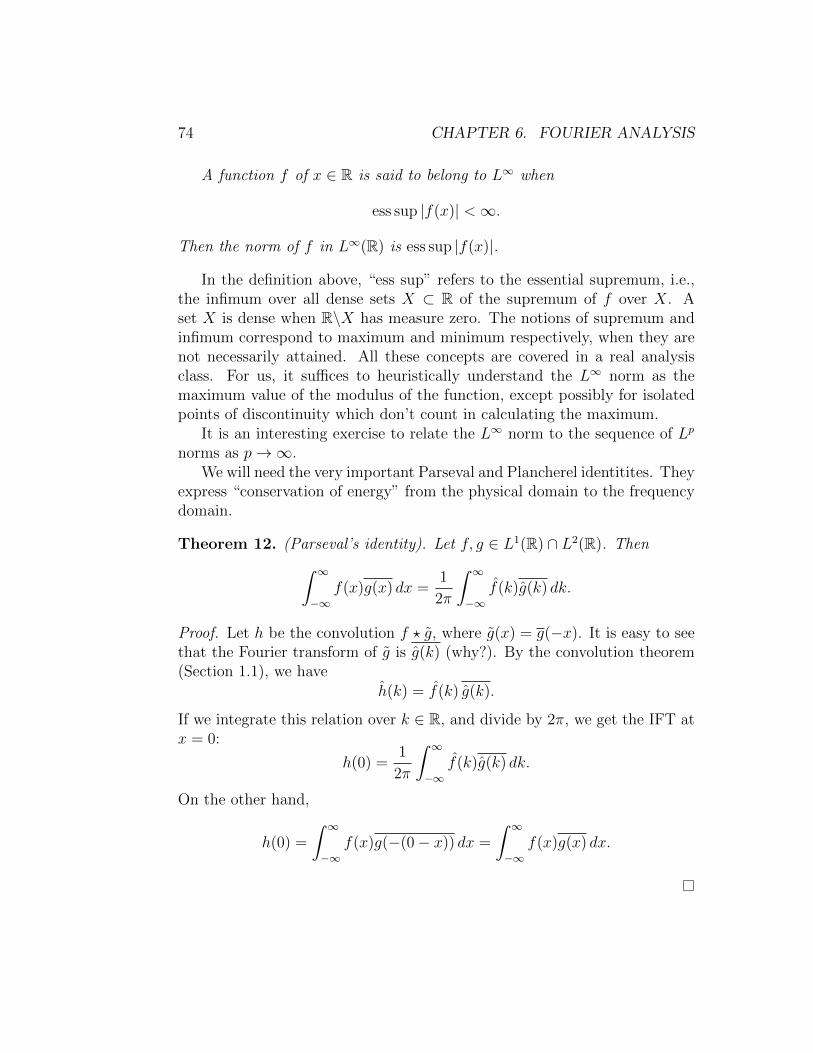
74 CHAPTER 6. FOURIER ANALYSIS
A function f of x ∈ R is said to belong to L∞ when
ess sup |f(x)| <∞.
Then the norm of f in L∞(R) is ess sup |f(x)|.
In the definition above, “ess sup” refers to the essential supremum, i.e.,the infimum over all dense sets X ⊂ R of the supremum of f over X. Aset X is dense when R\X has measure zero. The notions of supremum andinfimum correspond to maximum and minimum respectively, when they arenot necessarily attained. All these concepts are covered in a real analysisclass. For us, it suffices to heuristically understand the L∞ norm as themaximum value of the modulus of the function, except possibly for isolatedpoints of discontinuity which don’t count in calculating the maximum.
It is an interesting exercise to relate the L∞ norm to the sequence of Lp
norms as p→∞.We will need the very important Parseval and Plancherel identitites. They
express “conservation of energy” from the physical domain to the frequencydomain.
Theorem 12. (Parseval’s identity). Let f, g ∈ L1(R) ∩ L2(R). Then∫ ∞−∞
f(x)g(x) dx =1
2π
∫ ∞−∞
f(k)g(k) dk.
Proof. Let h be the convolution f ? g, where g(x) = g(−x). It is easy to seethat the Fourier transform of g is g(k) (why?). By the convolution theorem(Section 1.1), we have
h(k) = f(k) g(k).
If we integrate this relation over k ∈ R, and divide by 2π, we get the IFT atx = 0:
h(0) =1
2π
∫ ∞−∞
f(k)g(k) dk.
On the other hand,
h(0) =
∫ ∞−∞
f(x)g(−(0− x)) dx =
∫ ∞−∞
f(x)g(x) dx.

6.4. SMOOTHNESS AND TRUNCATION 75
Theorem 13. (Plancherel’s identity). Let f ∈ L1(R) ∩ L2(R). Then∫ ∞−∞|f(x)|2 dx =
1
2π
∫ ∞−∞|f(k)|2 dk.
Proof. Apply Parseval’s identity with g = f .
(With the help of these formulas, it is in fact possible to extend theirvalidity and the validity of the FT to f, g ∈ L2(R), and not simply f, g ∈L1(R) ∩ L2(R). This is a classical density argument covered in many goodanalysis texts.)
We need one more concept before we get to the study of truncation ofFourier transforms. It is the notion of total variation. We assume that thereader is familiar with the spaces Ck(R) of bounded functions which are ktimes continuously differentiable.
Definition 20. (Total variation) Let f ∈ C1(R). The total variation of f isthe quantity
‖f‖TV =
∫ ∞−∞|f ′(x)| dx. (6.9)
For functions that are not C1, the notion of total variation is given by eitherexpression
‖f‖TV = limh→0
∫ ∞−∞
|f(x)− f(x− h)||h|
dx = sup{xp} finite subset of R
∑p
|f(xp+1)−f(xp)|,
(6.10)These more general expressions reduce to
∫∞−∞ |f
′(x)| dx when f ∈ C1(R).When a function has finite total variation, we say it is in the space of func-tions of bounded variation, or BV(R).
The total variation of a piecewise constant function is simply the sum ofthe absolute value of the jumps it undergoes. This property translates to auseful intuition about the total variation of more general functions if we viewthem as limits of piecewise constant functions.
The important meta-property of the Fourier transform is that
decay for large |k| corresponds to smoothness in x.

76 CHAPTER 6. FOURIER ANALYSIS
There are various degrees to which a function can be smooth or rates atwhich it can decay, so therefore there are several ways that this assertioncan be made precise. Let us go over a few of them. Each assertion eitherexpresses a decay (in k) to smoothness (in x) implication, or the converseimplication.
• Let f ∈ L1(R) (decay), then f ∈ L∞(R) and f is continuous (smooth-ness). That’s because |eikx| = 1, so
|f(x)| ≤ 1
2π
∫|eikxf(k)| dk =
1
2π
∫|f(k)| dk,
which proves boundedness. As for continuity, consider a sequence yn →0 and the formula
f(x− yn) =1
2π
∫eik(x−yn)f(k) dk.
The integrand converges pointwise to eikxf(k), and is uniformly boundedin modulus by the integrable function |f(k)|. Hence Lebesgue’s dom-inated convergence theorem applies and yields f(x − yn) → f(x), i.e.,continuity in x.
• Let f(k)(1 + |k|p) ∈ L1(R) (decay). Then f ∈ Cp (smoothness). Wesaw the case p = 0 above; the justification is analogous in the generalcase. We write
|f (n)(x)| ≤ 1
2π
∫|eikx(ik)nf(k)| dk ≤
∫|k|n|f(k)| dk,
which needs to be bounded for all 0 ≤ n ≤ p. This is obviously thecase if f(k)(1 + |k|p) ∈ L1(R). Continuity of f (p) is proved like before.
• Let f ∈ BV(R) (smoothness). Then f(k) ≤ ‖f‖TV |k|−1 (decay). Iff ∈ C1 ∩BV (R), then this is justified very simply from (6.9), and
ikf(k) =
∫e−ikxf ′(x) dx.
Take a modulus on both sides, and get the desired relation
|k||f(k)| ≤∫|f ′(x)|dx = ‖f‖TV <∞.

6.4. SMOOTHNESS AND TRUNCATION 77
When f ∈ BV (R), but f /∈ C1, either of the more general formulas(6.10) must be used instead. It is a great practice exercise to articulatea modified proof using the limh→0 formula, and properly pass to thelimit.
• Let f such that f (k) ∈ L2(R) for 0 ≤ k < p, and assume that f (p) ∈BV(R) (smoothness). Then there exists C > 0 such that |f(k)| ≤|k|−p−1 (decay). This claim is also formulated as point (a) in Theo-rem 1 on page 30 of Trefethen’s “Spectral methods in Matlab”. Thejustification is very simple when f ∈ Cp+1: we then get
(ik)p+1f(k) =
∫e−ikxf (p+1)(x) dx,
so
|k|p+1|f(k)| ≤∫|f (p+1)(x)| dx = ‖f (p)‖TV <∞.
Again, it is a good exercise to try and extend this result to functionsnot in Cp+1.
• (This is the one we’ll use later). (Same proof as above.)
In summary, let f have p derivatives in L1. Then |f(k)| ≤ C|k|−p. Thisis the form we’ll make the most use of in what follows.
Example 21. The canonical illustrative example for the two statements in-volving bounded variation is that of the B-splines. Consider
s(x) =1
2χ[−1,1](x),
the rectangle-shaped indicator of [−1, 1] (times one half). It is a function inBV (R), but it has no derivative in L2(R). Accordingly, its Fourier transforms(k) is predicted to decay at a rate ∼ |k|−1. This is precisely the case, for weknow
s(k) =sin k
k.
Functions with higher regularity can be obtained by auto-convolution of s; forinstance s2 = s ? s is a triangle-shaped function which has one derivative in

78 CHAPTER 6. FOURIER ANALYSIS
L2, and such that s′2 ∈ BV (R). We anticipate that s2(k) would decay like|k|−2, and this the case since by the convolution theorem
s2(k) = (s(k))2 =
(sin k
k
)2
.
Any number of autoconvolutions s?s . . . ? s can thus be considered: that’s thefamily of B-splines.
The parallel between smoothness in x and decay in k goes much further.We have shown that p derivatives in x very roughly corresponds to an inverse-polynomial decay |k|−p in k. So C∞ functions in x have so called super-algebraic decay in k: faster than Cp|k|−p for all p ≥ 0.
The gradation of very smooth functions goes beyond C∞ functions toinclude, in order:
• analytic functions that can be extended to a strip in the complex plane(like f(x) = 1/(1+x2)), corresponding to a Fourier transform decayingexponentially (in this case f(k) = πe−|k|). That’s Paley-Wiener theory,the specifics of which is not material for this course.
• analytic functions that can be extended to the whole complex planewith super-exponential growth (like f(x) = e−x
2/2), whose Fouriertransform decays faster than exponentially (in this case f(k) =
√π/2e−k
2/2).
• analytic functions that can be extended to the whole complex planewith exponential growth at infinity (like f(x) = sinx
x), whose Fourier
transform is compactly supported (in this case f(k) = 2πχ[−1,1](k)).That’s Paley-Wiener theory in reverse. Such functions are also calledbandlimited.
More on this in Chapter 4 of Trefethen’s book.An important consequence of a Fourier transform having fast decay is
that it can be truncated to some large interval k ∈ [−N,N ] at the expenseof an error that decays fast as a function of N . The smoother f , the fasterf decays, and the more accurate the truncation to large N in frequency. Onthe other hand, there may be convergence issues if f(x) is not smooth.
To make this quantitative, put
fN(k) = χ[−N,N ](k)f(k).

6.4. SMOOTHNESS AND TRUNCATION 79
Recall that 12π
∫ N−N e
ikxdx = sin(Nx)πx
. By the convolution theorem, we thereforehave
fN(x) =sinNx
πx? f(x).
In the presence of f ∈ L2(R), letting N →∞ always gives rise to conver-gence fN → f in L2(R). This is because by Plancherel’s identity,
‖f − fN‖22 =1
2π
∫ ∞−∞|fN(k)− f(k)|2 dk =
1
2π
∫|k|>N
|f(k)|2 dk.
This quantity tends to zero as N →∞ since the integral∫R |f(k)|2 over the
whole line is bounded.The story is quite different if we measure convergence in L∞ instead of
L2, when f has a discontinuity. Generically, L∞ (called uniform) convergencefails in this setting. This phenomenon is called Gibb’s effect, and manifestsitself through ripples in reconstructions from truncated Fourier transforms.Let us illustrate this on the Heaviside step function
u(x) =
{1 if x ≥ 0;0 if x < 0.
(It is not a function in L2(R) but this is of no consequence to the argument.It could be modified into a function in L2(R) by some adequate windowing.)Since u(x) is discontinuous, we expect the Fourier transform to decay quiteslowly. Consider the truncated FT
uN(k) = χ[−N,N ](k)u(k).
Back in the x domain, this is
uN(x) =sinNx
πx? u(x)
=
∫ ∞0
sinN(x− y)
π(x− y)dy
=
∫ Nx
−∞
sin y
πydy
≡ s(Nx).
(Draw picture)

80 CHAPTER 6. FOURIER ANALYSIS
The function s(Nx) is a sigmoid function going from 0 at −∞ to 1 at∞,going through s(0) = 1/2, and taking on min. value ' −.045 at x = −π/Nand max. value ' 1.045 at x = π/N . The oscillations have near-period π/N .The parameter N is just a dilation index for the sigmoid, it does not changethe min. and max. values of the function. Even as N →∞, there is no waythat the sigmoid would converge to the Heaviside step in a uniform manner:we always have
‖u− uN‖∞ & .045.
This example of Gibb’s effect goes to show that truncating Fourier expan-sions could be a poor numerical approximation if the function is nonsmooth.
However, if the function is smooth, then everything goes well. Let usstudy the decay of the approximation error
ε2N = ‖f − fN‖22for truncation of the FT to [−N,N ]. Again, we use Plancherel to get
ε2N =
∫|k|>N
|f(k)|2 dk
Now assume that f(k) ≤ C|k|−p, a scenario already considered earlier. Then
ε2N ≤ C
∫|k|>N
|k|−2p ≤ C ′N−2p+1,
so, for some constant C ′′ (dependent on p but independent of N , hence calledconstant),
εN ≤ C ′′N−p+1/2.
The larger p, the faster the decay as N →∞.When a function is C∞, the above decay rate of the approximation error
is valid for all p > 0. When the function is analytic and the Fourier trans-form decays exponentially, the decay rate of the approximation error is evenfaster, itself exponential (a good exercise). In numerical analysis, either suchbehavior is called spectral accuracy.
6.5 Chebyshev expansions
Chebyshev expansions, interpolation, differen-tiation, and quadrature rules are not part ofthe material for 18.330 in 2012.

6.5. CHEBYSHEV EXPANSIONS 81
In the previous sections, we have seen that smooth functions on the realline have fast decaying Fourier transforms.
On a finite interval, a very similar property hold for Fourier series: if afunction is smooth in [−π, π] and connects smoothly by periodicity at x = −πand x = π, then its Fourier series (6.5) decays fast. Periodicity is essential,because the points x = −π and x = π play no particular role in (6.5). Theymight as well be replaced by x = 0 and x = 2π for the integration bounds.So if a function is to qualify as smooth, it has to be equally smooth at x = 0as it is at x = −π, identified with x = π by periodicity.
For instance if a function f is smooth inside [−π, π], but has f(−π) 6=f(π), then for the purpose of convergence of Fourier series, f is considereddiscontinuous. We know what happens in this case: the Gibbs effect takesplace, partial inverse Fourier series have unwelcome ripples, and convergencedoes not occur in L∞.
If f is smooth and periodic, then it is a good exercise to generalize theconvergence results of the previous section, from the Fourier transform toFourier series.
How shall we handle smooth functions in intervals [a, b], which do notconnect smoothly by periodicity? The answer is not unique, but the moststandard tool for this in numerical analysis are the Chebyshev polynomials.
For simplicity consider x ∈ [−1, 1], otherwise rescale the problem. Takea Ck nonperiodic f(x) in [−1, 1]. The trick is to view it as g(θ) = f(cos θ).Since cos[0, π] = cos[π, 2π] = [−1, 1], all the values of x ∈ [−1, 1] are coveredtwice by θ ∈ [0, 2π]. Obviously, at any point θ, g inherits the smoothness off by the chain rule. Furthermore, g is periodic since cos θ is periodic. So g isexactly the kind of function which we expect should have a fast convergingFourier series:
gk =
∫ 2π
0
e−ikθg(θ) dθ, g(θ) =1
2π
∞∑k=−∞
eikθgk, k ∈ Z.
Since g(θ) is even in θ, we may drop the sin θ terms in the expansion, as wellas the negative k:
gk =
∫ 2π
0
cos (kθ)g(θ) dθ, g(θ) =1
2πg0 +
1
π
∞∑k=1
cos (kθ)gk, k ∈ Z+.

82 CHAPTER 6. FOURIER ANALYSIS
Back to f , we find
gk = 2
∫ 1
−1cos (k arccosx)f(x)
dx√1− x2
, f(x) =1
2πg0+
1
π
∞∑k=1
cos (k arccosx)gk, k ∈ Z+.
The function cos(k arccosx) happens to be a polynomial in x, of orderk, called the Chebyshev polynomial of order k. Switch to the letter n as isusually done:
Tn(x) = cos(n arccosx), x ∈ [−1, 1].
The first few Chebyshev polynomials are
T0(x) = 1, T1(x) = x, T2(x) = 2x2 − 1.
It is a good exercise (involving trigonometric identities) to show that theyobey the recurrence relation
Tn+1(x) = 2xTn(x)− Tn−1(x).
The orthogonality properties of Tn(x) over [−1, 1] follows from those ofcos(nθ) over [0, π], but watch the special integration weight:∫ 1
−1Tm(x)Tn(x)
dx√1− x2
= cnδmn,
with cn = π/2 if n = 0 and cn = π otherwise. The Chebyshev expansion off is therefore
〈f, Tn〉 =
∫ 1
−1Tn(x)f(x)
dx√1− x2
, f(x) =1
π〈f, T0〉+
2
π
∞∑n=1
Tn(x)〈f, Tn〉, k ∈ Z+.
Under the hood, this expansion is the FS of a periodic function, so we canapply results pertaining to Fourier series and Fourier transforms to obtainfast decay of Chebyshev expansions. This way, spectral accuracy is restoredfor nonperiodic functions defined on an interval.
Chapter 7
Spectral Interpolation,Differentiation, Quadrature
7.1 Interpolation
7.1.1 Bandlimited interpolation
While equispaced points generally cause problems for polynomial interpola-tion, as we just saw, they are the natural choice for discretizing the Fouriertransform. For data on xj = jh, j ∈ Z, recall that the semidiscrete Fouriertransform (SFT) and its inverse (ISFT) read
f(k) = h∑j∈Z
e−ikxjfj, fj =1
2π
∫ π/h
−π/heikxj f(k) dk.
The idea of spectral interpolation, or bandlimited interpolation, is to evaluatethe ISFT formula above at some point x not equal to one of the xj.
Definition 21. (Fourier/spectral/bandlimited interpolation on R) Let xj =
jh, j ∈ Z. Consider f : R 7→ R, its restriction fj = f(xj), and the SFT f(k)of the samples fj. Then the spectral interpolant is
p(x) =1
2π
∫ π/h
−π/heikxf(k) dk.
We can view the formula for p(x) as the inverse Fourier transform of thecompactly supported function equal to f(k) for k ∈ [−π/h, π/h], and zero
83

84CHAPTER 7. SPECTRAL INTERPOLATION, DIFFERENTIATION, QUADRATURE
otherwise. When the Fourier transform of a function is compactly supported,we say that that function is bandlimited, hence the name of the interpolationscheme.
Example 22. Let
fj = δ0j =
{1 if j = 0;0 if j 6= 0.
Then the SFT is f(k) = h for k ∈ [−π/h, π/h] as we saw previously. Extendit to k ∈ R by zero outside of [−π/h, π/h]. Then
p(x) =sin(πx/h)
πx/h= sinc(πx/h).
This function is also called the Dirichlet kernel. It vanishes at xj = jh forj 6= 0, integer.
Example 23. In full generality, consider now the sequence
fj =∑k∈Z
δjkfk.
By linearity of the integral,
p(x) =∑k∈Z
fksinc(π(x− xk)/h).
The interpolant is a superposition of sinc functions, with the samples fj asweights. Here sinc is the analogue of the Lagrange elementary polynomialsof a previous section, and is called the interpolation kernel. For this reason,bandlimited interpolation sometimes goes by the name Fourier-sinc interpo-lation.
(Figure here for the interpolation of a discrete step.)
In the example above we interpolate a discontinuous function, and theresult is visually not very good. It suffers from the same Gibbs effect thatwe encountered earlier. The smoother the underlying f(x) which fj are thesamples of, however, the more accurate bandlimited interpolation.
In order to study the approximation error of bandlimited interpolation,we need to return to the link between SFT and FT. The relationship be-tween p(x) and fj is sampling, whereas the relationship between the FT

7.1. INTERPOLATION 85
f(k)χ[−π/h,π/h](k) and the SFT f(k) is periodization. We have already alludedto this correspondence earlier, and it is time to formulate it more precisely.
(Figure here; sampling and periodization)
Theorem 14. (Poisson summation formula, FT version) Let u : R 7→ R,sufficiently smooth and decaying sufficiently fast at infinity. (We are delib-erately imprecise!) Let vj = u(xj) for xj = jh, j ∈ Z, and
u(k) =
∫Re−ikxu(x) dx, (FT ), k ∈ R,
v(k) = h∑j∈Z
e−ikxju(xj). (SFT ), k ∈ [−π/h, π/h].
Then
v(k) =∑m∈Z
u(k +m2π
h), k ∈ [−π/h, π/h] (7.1)
In some texts the Poisson summation formula is written as the specialcase k = 0:
h∑j∈Z
u(jh) =∑m∈Z
u(2π
hm).
Exercise: use what we have already seen concerning translations and Fouriertransforms to show that the above equation implies (hence is equivalent to)equation (7.1).
Proof. Consider the right-hand side in (7.1), and call it
φ(k) =∑m∈Z
u(k +m2π
h), k ∈ [−π/h, π/h].
It suffices to show that φ(k) = v(k), or equivalently in terms of their ISFT,that φj = vj for j ∈ Z. The ISFT is written
φj =1
2π
∫ π/h
−π/h
[∑m∈Z
u(k +m2π
h)
]eikjh dk.

86CHAPTER 7. SPECTRAL INTERPOLATION, DIFFERENTIATION, QUADRATURE
The function u is smooth, hence integrable, and the sum over m convergesfast. So we can interchange sum and integral:
φj =1
2π
∑m∈Z
∫ π/h
−π/hu(k +m
2π
h)eikjh dk.
Now put k′ = k +m2πh
, and change variable:
φj =1
2π
∑m∈Z
∫ πh−m 2π
h
−πh−m 2π
h
u(k′)eik′jhe−i
2πhjh dk′.
The extra exponential factor e−i2πhjh is equal to 1 because j ∈ Z. We are
in presence of an integral over R chopped up into pieces corresponding tosub-intervals of length 2π/h. Piecing them back together, we get
φj =1
2π
∫Ru(k′)eik
′jhdk′,
which is exactly the inverse FT of u evaluated at xj = jh, i.e., φj = u(xj) =vj.
The Poisson summation formula shows that sampling a function at rateh corresponds to periodizing its spectrum (Fourier transform.) with a period2π/h. So the error made in sampling a function (and subsequently doingbandlimited interpolation) is linked to the possible overlap of the Fouriertransform upon periodization.
• Scenario 1. Assume supp(u) ⊂ [−π/h, π/h]. Then no error is made insampling and interpolating u at rate h, because nothing happens upon2π/h-periodization and windowing into [−π/h, π/h]:
p(k) = u(k) ⇒ p(x) = u(x).
(Draw picture)
• Scenario 2. Now assume that u(k) is not included in [−π/h, π/h].In general the periodization of u(k) will result in some overlap inside[−π/h, π/h]. We call this aliasing. In that case, some information islost and interpolation will not be exact.

7.1. INTERPOLATION 87
Scenario 1 is known as the Shannon sampling theorem: a function ban-dlimited in [−π/h, π/h] in k space is perfectly interpolated by bandlimitedinterpolation, on a grid of spacing h or greater. In signal processing h is alsocalled the sampling rate, because x has the interpretation of time. When his the largest possible rate such that no aliasing occurs, it can be referred toas the Nyquist rate.
More generally, the accuracy of interpolation is linked to the smoothnessof u(x). If the tails u(k) are small and h is large, we can expect that theerror due to periodization and overlap won’t be too big. The following resultis a consequence of the Poisson summation formula.
Theorem 15. (Error of bandlimited interpolation) Let u have p ≥ 1 deriva-tives in L1(R). Let vj = u(xj) at xj = jh, j ∈ Z. Denote by p(x) thebandlimited interpolant formed form vj. Then, as h→ 0,
|u(k)− p(k)| = O(hp) |k| ≤ π
h,
and‖u− p‖2 = O(hp−1/2).
Proof. Denote by u(k) the FT of u(x), and by v(k) the SFT of vj, so thatp(k) = v(k) on [−π/h, π/h]. By the Poisson summation formula (7.1),
v(k)− u(k) =∑m6=0
u(k +m2π
h), k ∈ [−π/h, π/h].
As we saw earlier, the smoothness condition on u imply that
|u(k)| ≤ C |k|−p.
Since
k +m2π
h∈ [−π
h+m
2π
h,π
h+m
2π
h],
we have |k +m2πh| ≥ |mπ
h|, hence
|u(k +m2π
h)| ≤ C ′ |mπ
h|−p,
for some different constant C ′. Summing over m 6= 0,
|v(k)− u(k)| ≤ C ′∑m 6=0
|m|−p(πh
)−p ≤ C ′′ (π
h)−p ≤ C ′′′ hp.

88CHAPTER 7. SPECTRAL INTERPOLATION, DIFFERENTIATION, QUADRATURE
One can switch back to the x domain by means of the Plancherel formula
‖u− p‖2L2 =1
2π‖u(k)− v(k)‖2L2(R).
The right-hand side contains the integral of |u(k)− v(k)|2 over R. Break thisintegral into two pieces:
• Over [−π/h, π/h], we have seen that |u(k) − v(k)|2 = O(h2p). Theintegral is over an interval of length O(1/h), hence the L2 norm squaredis O(h2p−1). Taking a square root to get the L2 norm, we get O(hp−1/2).
• For |k| ≥ π/h, we have p(k) = 0, so it suffices to bound∫|k|≥π/h |u(k)|2 dk.
Since |u(k)| ≤ C |k|−p, this integral is bounded by O((π/h)2p−1). Tak-ing a square root, we again obtain a O(hp−1/2).
We have seen how to interpolate a function defined on R, but as a closingremark let us notice that a similar notion exists for functions defined onintervals, notably x ∈ [−π, π] or [0, 2π]. In that case, wavenumbers arediscrete, the FT is replaced by the FS, and the SFT is replaced by the DFT.Evaluating the DFT for x not on the grid would give an interpolant:
1
2π
N/2∑k=−N/2+1
eikxfk.
Contrast with the formula (6.8) for the IDFT. This is almost what we want,but not quite, because the highest wavenumber k = N/2 is treated asym-metrically. It gives rise to an unnatural complex term, even if fk is real andeven. To fix this, it is customary to set f−N/2 = fN/2, to extend the sumfrom −N/2 to N/2, but to halve the terms corresponding to k = −N/2 andN/2. We denote this operation of halving the first and last term of a sumby a double prime after the sum symbol:∑′′
Itis easy to check that this operation does not change the interpolating prop-erty. The definition of bandlimited interpolant becomes the following in thecase of intervals.

7.1. INTERPOLATION 89
Definition 22. (Spectral interpolation on [0, 2π]) Let xj = jh, j = 0, . . . , N−1 with h = 1/N . Consider f : [0, 2π] 7→ R, its restriction fj = f(xj), and
the DFT fk of the samples fj. Then the spectral interpolant is
p(x) =1
2π
∑′′ N/2
k=−N/2eikxfk.
Because p(x) is a superposition of “monomials” of the form eikx = (eix)k
for k integer, we call it a trigonometric polynomial.The theory for interpolation by trigonometric polynomials (inside [0, 2π])
is very similar to that for general bandlimited interpolants. The only impor-tant modification is that [0, 2π] is a periodized interval, so a function qualifiesas smooth only if it connects smoothly across x = 0 indentified with x = 2πby periodicity. The Poisson summation formula is still the central tool, andhas a counterpart for Fourier series.
Theorem 16. (Poisson summation formula, FS version) Let u : [0, 2π] 7→ R,sufficiently smooth. Let vj = u(θj) for θj = jh, j = 1, . . . , N , h = 2π/N ,and
uk =
∫ 2π
0
e−ikθu(θ) dθ, (FS), k ∈ Z,
vk = hN∑j=1
e−ikθju(θj). (DFT ), k = −N2, . . . ,
N
2− 1.
Then
vk =∑m∈Z
uk+mN , k = −N2, . . . ,
N
2− 1. (7.2)
(Recall that N = 2πh
so this formula is completely analogous to (7.1).)
For us, the important consequence is that if u has p derivatives in L1,over the periodized interval [0, 2π], then the bandlimited interpolation erroris a O(hp) in the pointwise sense in k space, and O(hp−1/2) in the L2 sense.
For this result to hold it is important that u has p derivatives at theorigin as well (identified by periodicity with 2π), i.e., the function is equallysmooth as it straddles the point where the interval wraps around by pe-riodicity.Otherwise, if u(θ) has discontinuities such as. u(2π−) 6= u(0+),interpolation will suffer from the Gibbs effect.

90CHAPTER 7. SPECTRAL INTERPOLATION, DIFFERENTIATION, QUADRATURE
7.1.2 Chebyshev interpolation
Consider now smooth functions inside [−1, 1] (for illustration), but not nec-essarily periodic. So the periodization
∑j f(x + 2j) may be discontinuous.
Polynomial interpolation on equispaced points may fail because of the Rungephenomenon, and bandlimited interpolation will fail due to Gibbs’s effect.
A good strategy for interpolation is the same trick as the one we used fortruncation in the last chapter: pass to the variable θ such that
x = cos θ.
Then x ∈ [−1, 1] corresponds to θ ∈ [0, π]. We define g(θ) = f(cos θ) with g2π-periodic and even.
We can now consider the bandlimited interpolant of g(θ) on an equispacedgrid covering [0, 2π], like for instance
θj =πj
N, where j = 1, . . . , 2N.
Using the definition we saw at the end of the last section (with the ”doubleprime”), we get
q(θ) =1
2π
∑′′ N
k=−Neikθgk, gk =
π
N
2N−1∑j=0
e−ikθjg(θj).
By even symmetry in θ and k (why?), we can write
q(θ) =N∑k=0
cos(kθ)ck,
with
c0 =g02π, ck =
gkπ
for k 6= 0.
Note that the ck are determined from the samples g(θj).Back to x, we get the sample points xj = cos(θj). They are called Cheby-
shev points. They are not equispaced anymore, and because they are theprojection on the x-axis of equispaced points on the unit circle, they clusternear the edges of [−1, 1]. There are N + 1 of them, from j = 0 to N , becauseof the symmetry in θ. It turns out that the xj are the extremal points of the

7.1. INTERPOLATION 91
Chebyshev polynomial TN(x), i.e., the points in [−1, 1] where TN takes itsmaximum and minimum values.
In terms of the variable x, the interpolant can be expressed as
p(x) = q(acos x) =N∑n=0
Tn(x)cn, Tn(x) = cos(n acos x),
with the same cn as above. Since Tn(x) are polynomials of degree 0 ≤ n ≤ N ,and p(x) interpolates f(x) at the N + 1 (non-equispaced) points xj, we arein presence of the Lagrange interpolation polynomial for f at xj!
In practice, the formula in terms of Tn(x) may not even be needed. Frominterpolation points xj, it suffices to map them to θj = acos xj, then getthe interpolated values as q(acos xj). For instance, when xj are Chebyshevpoints on a grid twice finer than xj, namely xj = acos πj
2Nfor j = 1, . . . , 4N ,
it is a good exercise to write a fast FFT-based algorithm for Chebyshevinterpolation.
The interesting conclusion is that, although this is a polynomial inter-polant, the error analysis is inherited straight from Fourier analysis. If f issmooth, then g is smooth and periodic, and we saw that the bandlimitedinterpolant converges very fast. The Chebyshev interpolant of f is equal tothe bandlimited interplant of g so it converges at the exact same rate (in L∞
in k or n space) — for instance O(N−p−1) when f has p derivatives (in BV).In particular, we completely bypassed the standard analysis of error of
polynomial interpolation, and proved universal convergence for smooth f .The factor
πN+1(x) =N∏j=0
(x− xj)
that was posing problems in the error estimate then does not pose a problemanymore, because of the very special choice of Chebyshev points cos(πj/N)for the interpolation. Intuitively, clustering the grid points near the edgesof the interval [−1, 1] helps giving πN+1(x) more uniform values throughout[−1, 1], hence reduces the gross errors near the edges.
Let us now explain the differences in the behavior of the monic polynomial∏Nj=0(x−xj) for equispaced vs. Chebyshev points, and argue that Chebyshev
points are near-ideal for interpolation of smooth functions in intervals. Thediscussion below is mostly taken from Trefethen, p.43. (See also the lastproblem on homework 2 for an example of different analysis.)
92CHAPTER 7. SPECTRAL INTERPOLATION, DIFFERENTIATION, QUADRATURE
Let p(z) =∏N
j=0(z − xj), where we have extended the definition of themonic polynomial to z ∈ C. We compute
log |p(z)| =N∑j=0
log |z − xj|,
Put
φN(z) = (N + 1)−1N∑j=0
log |z − xj|.
The function φN is like an electrostatic potential, due to charges at z = xj,each with potential (N + 1)−1 log |z − xj|. Going back to p(z) from φN iseasy:
p(z) = e(N+1)φN (z).
Already from this formula, we can see that small variations in φN will leadto exponentially larger variations in p(z), particularly for large N .
Let us now take a limit N → ∞, and try to understand what happenswithout being too rigorous. What matters most about the Chebyshev pointsis their density : the Chebyshev points are the projection onto the real-axisof a sequence of equispaced points on a circle. If the density of points on thecircle is a constant 1/(2π), then the density of points on [−1, 1] generated byvertical projection is
ρCheb(x) =1
π√
1− x2. (normalized to integrate to 1 on [−1, 1])
(This is a density in the sense that
N
∫ b
a
ρCheb(x) dx
approximately gives the number of points in [a, b].) Contrast with a uniformdistribution of points, with density
ρequi(x) =1
2.
Then the potential corresponding to any given ρ(x) is simply
φ(z) =
∫ 1
−1ρ(x) log |z − x| dx.
The integral can be solved explicitly for both densities introduced above:

7.1. INTERPOLATION 93
• For ρequi, we get
φequi(z) = −1 +1
2Re((z + 1) log(z + 1)− (z − 1) log(z − 1)).
It obeys φequi(0) = −1, φequi(±1) = −1 + log 2.
• For ρCheb, we get
φCheb(z) = log|z −√z2 − 1|2
.
This function obeys (interesting exercise) φCheb(x) = − log 2 for allx ∈ [−1, 1] on the real axis.
The level curves of both φequiv and φCheb in the complex plane are shownon page 47 of Trefethen.
Overlooking the fact that we have passed to a continuum limit for thepotentials, we can give a precise estimate on the monic polynomial:
|pequi(z)| ' e(N+1)φequi(z) =
{(2/e)N near x = ±1;(1/e)N near x = 0.
whereas
|pCheb(z)| ' e(N+1)φequi(z) = 2−N , z ∈ [−1, 1].
We see that pequi can take on very different values well inside the intervalvs. near the edges. On the other hand the values of pCheb are near-constant in[−1, 1]. The density ρCheb(x) is the only one that will give rise to this behav-ior, so there is something special about it. It is the difference in asymptoticbehavior of (2/e)−N vs. 2−N that makes the whole difference for interpola-tion, as N →∞.
One may argue that neither pequi nor pCheb blow up as N → ∞, but itis an interesting exercise to show that if we were interpolating in an interval[−a, a] instead of [−1, 1], then the bounds would be multiplied by aN , byhomogeneity.
The Chebyshev points are not the only one that correspond to the densityρCheb(x) as N →∞. For instance, there is also the Chebyshev roots
θ′j =π
2N+πj
N, j = 0, . . . , 2N − 1,

94CHAPTER 7. SPECTRAL INTERPOLATION, DIFFERENTIATION, QUADRATURE
which are the roots of TN(x), instead of being the extremal points. Theygive rise to very good interpolation properties as well.
Finally, let us mention that the theory can be pushed further, and thatthe exponential rate of convergence of Chebyshev interpolation for analyticfunctions can be linked to the maximum value of φ(z) on the strip in whichthe extension f(z) of f(x) is analytic. We will not pursue this further.
7.2 Differentiation
7.2.1 Bandlimited differentiation
The idea that a numerical approximation of a derivative can be obtained fromdifferentiating an interpolant can be pushed further. In this section we returnto bandlimited interpolants. We’ve seen that they are extremely accuratewhen the function is smooth and periodic; so is the resulting differentiationscheme. It is called bandlimited differentiation, or spectral differentiation.
First consider the case of x ∈ R and xj = jh, j ∈ Z. As we’ve seen, thebandlimited/spectral interpolant of u(xj) is
p(x) =1
2π
∫ π/h
−π/heikxu(k) dk,
where v(k) is the SFT of vj = u(xj). Differentiating p(x) reduces to amultiplication by ik in the Fourier domain. Evaluating p′(xj) is then just amatter of letting x = xj in the resulting formula. The sequence of steps forbandlimited differentiation (x ∈ R) is the following:
• Obtain the SFT v(k) of vj = u(xj);
• Multiply v(k) by ik;
• Obtain the ISFT of w(k) = ikv(k), call it wj.
The numbers wj obtained above are an approximation of u′(xj). Thefollowing result makes this precise.
Theorem 17. (Accuracy of bandlimited differentiation, see also Theorem 4in Trefethen’s book) Let u have p derivatives in L1(R). Let vj = u(xj), andwj = p′(xj) be the result of bandlimited differentiation. Then
supj|wj − u′(xj)| = O(hp−2).

7.2. DIFFERENTIATION 95
and‖u′ − p′‖2 = O(hp−3/2).
Proof. The proof hinges on the fact that
|v(k)− u(k)| = O(hp).
One power of h is lost when differentiating u (because ik is on the order of1/h over the fundamental cell [−π/h, π/h]). Half a power of h is lost in goingback to the physical domain (j instead of k) via the L2 norm (why?), and afull power of h is lost when going back to j in the uniform sense (why?).
The point of the above theorem is that the order of bandlimited differ-entiation is directly linked to the smoothness of the function, and can bearbitrarily large. This is called spectral accuracy. One can even push theanalysis further and show that, when f is real-analytic, then the rate ofconvergence of wj towards u′(xj) is in fact exponential/geometric.
Of course in practice we never deal with a function u(x) defined on thereal line. In order to formulate an algorithm, and not simply a sequence ofabstract steps, we need to limit the interval over which u is considered. Spec-tral differentiation in the periodic interval [0, 2π] works like before, exceptDFT are substituted for SFT. For θ ∈ [0, 2π], we’ve seen that the spectralinterpolant is defined as
p(θ) =1
2π
∑′′ N/2
k=−N/2eikθfk.
(The double prime is important here.) Again, a derivative can be imple-mented by multiplying by ik in the Fourier domain. The sequence of stepsis very similar to what it was before, except that we can now label them as“compute”, and not just “obtain”:
• Compute the DFT vk of vj = u(xj);
• Multiply vk by ik;
• Compute the IDFT of wk = ikvk, call it wj.
The result of accuracy are the same as before, with the provision that u needsto be not only smooth, but also smooth when extended by periodicity.
The FFT can be used to yield a fast O(N logN) algorithm for spectraldifferentiation.
Note that higher derivatives are obtained in the obvious manner, by mul-tiplying in Fourier by the adequate power of ik.

96CHAPTER 7. SPECTRAL INTERPOLATION, DIFFERENTIATION, QUADRATURE
7.2.2 Chebyshev differentiation
In view of what has been covered so far, the idea of Chebyshev differentiationis natural: it is simply differentiation of the Chebyshev interpolant at theChebyshev nodes. It proves very useful for those smooth functions on aninterval, which do not necessarily extend smoothly by periodicity.
Let us recall that the Chebyshev interpolant is q(x) = p(arccosx), wherep(θ) is the bandlimited interpolant of u(cos θj) at the Chebyshev pointsxj = cos θj. As such, a differentiation on q(x) is not the same thing as adifferentiation on p(θ). Instead, by the chain rule,
q′(x) =−1√
1− x2p′(arccosx).
The algorithm is as follows. Start from the knowledge of u(xj) at xj =cos θj, θj = jh, h = π/N , and j = 1, . . . , N .
• Perform an even extension of u(xj) to obtain u(cos θj) for θj = jh,h = π/N , and j = −N + 1, . . . , N . Now we have all the equispacedsample of the periodic function u(cos θ) for θj covering [0, 2π], not just[0, π].
• Take the DFT of those samples, call it vk,
• Multiply by ik,
• Take the IDFT of the result ikvk,
• Multiply by −1/√
1− x2j to honor the chain rule. At the endpoints
xj = −1 or 1, take a special limit to obtain the proper values of p′(−1)and p(1). See Trefethen’s book for the correct values.
This is a fast algorithm since we can use the FFT for the DFT and IDFT.Since we are only a change of variables away from Fourier analysis in a pe-
riodic domain, the accuracy of Chebyshev differentiation is directly inheritedfrom that of bandlimited differentiation. We also have spectral accuracy.
Note that higher derivatives can be treated similarly, by applying thechain rule repeatedly.
In practice, Chebyshev methods are particularly useful for boundary-value problems (we’ll come back to this), when all samples of a function areto be determined at once, and when we have the freedom of choosing thesample points.

7.3. INTEGRATION 97
7.3 Integration
7.3.1 Spectral integration
To go beyond methods of finite order, the idea of spectral integration is tointegrate a bandlimited interpolant. This strategy yields very high accuracywhen the function is smooth and periodic.
Consider a function u(θ), θ ∈ [0, 2π]. Its samples are vj = u(θj) withθj = jh, h = 2π/N , and j = 1, . . . , N . Form the DFT:
vk = hN∑j=1
e−ikθjvj,
and the bandlimited interpolant,
p(θ) =1
2π
∑′′N/2
k=−N/2eikθvk.
Integrating p(θ) gives the remarkably simple following result.
∫ 2π
0
p(θ) dθ = v0 = hN∑j=1
u(θj).
We are back to the trapezoidal rule! (The endpoints are identified, θ0 = θN .)While we have already encountered this quadrature rule earlier, it is nowderived from Fourier analysis. So the plot thickens concerning its accuracyproperties.
Specifically, we have to compare v0 to u0 =∫ 2π
0u(θ) dθ, where uk are the
Fourier series coefficients of u(θ). The relationship between v0 and u0 is thePoisson summation formula (7.2):
v0 =∑m∈Z
umN , N =2π
h.
The most important term in this sum is u0 for m = 0, and our task is againto control the other ones, for m 6= 0. The resulting accuracy estimate is thefollowing.

98CHAPTER 7. SPECTRAL INTERPOLATION, DIFFERENTIATION, QUADRATURE
Theorem 18. Assume u has p derivatives in L1[0, 2π], where [0, 2π] is con-sidered a periodic interval. (So it matters that the function connects smoothlyby periodicity.) Then∫ 2π
0
u(θ) dθ − hN∑j=1
u(θj) = O(hp).
Proof. By the Poisson summation formula, in the notations of the precedingfew paragraphs,
u0 − v0 =∑m6=0
umN .
We have already seen that the smoothness properties of u are such that
|uk| ≤ C|k|−p.
So we have|u0 − v0| ≤ C
∑m 6=0
(mN)−p ≤ C ′N−p,
which is a O(hp).
As a conclusion, the trapezoidal rule is spectrally accurate (error O(hp+1)for all p ≥ 0 when u ∈ C∞), provided the function to be integrated insmooth and periodic. If the function is C∞ in an interval but is for instancediscontinuous upon periodization, then we revert to the usual O(h2) rate. Sothe true reason for the trapezoidal rule generally being O(h2) and not O(h∞)is only the presence of the boundaries!
An important example of such periodic smooth function, is a regularC∞function multiplied by a C∞ window that goes smoothly to zero at theendpoints of [a, b], like for instance a member of a partition of unity. (Thisplays an important role in some electromagnetism solvers, for computing theradar cross-section of scatterers.)
7.3.2 Chebyshev integration
Like for Chebyshev differentiation, we can warp θ into x by the formulaθ = arccosx, and treat smooth functions that are not necessarily periodic.Integrating a Chebyshev interpolant gives rise to Chebyshev integration, alsocalled Clenshaw-Curtis quadrature.

7.3. INTEGRATION 99
Assume that f(x) is given for x ∈ [−1, 1], otherwise rescale the x variable.The Chebyshev interpolant is built from the knowledge of f at the Chebyshevnodes xj = cos θj, and takes the form
p(x) =∑n≥0
anTn(x).
We have seen that an are obtained by even extension of f(xj), followed byan FFT where the sine terms are dropped. As a result,∫ 1
−1p(x) dx =
∑n≥0
an
∫ 1
−1Tn(x) dx.
We compute ∫ 1
−1Tn(x) dx =
∫ π
0
cos(nθ) sin θdθ.
This integral can be evaluated easily by relating cos and sin to complexexponentials (or see Trefethen’s book for an elegant shortcut via complexfunctions), and the result is∫ 1
−1Tn(x) dx =
{0 if n is odd;
21−n2 if n is even.
The algorithm for Chebyshev differentiation is simply: (1) find the coef-ficients an for 0 ≤ n ≤ N , and (2) form the weighted sum∑
n even, n≤N
an2
1− n2.
The accuracy estimate of Chebyshev integration is the same as that ofbandlimited integration, except we do not need periodicity. So the methodis spectrally accurate.
An important method related to Chebyshev quadrature is Gaussian quadra-ture, which is similar but somewhat different. It is also spectrally accurate forsmooth functions. Instead of using extrema or zeros of Chebyshev polynomi-als, it uses zeros of Legendre polynomials. It is usually derived directly fromproperties of orthogonal polynomials and their zeros, rather than Fourieranalysis. This topic is fascinating but would take us a little too far.