1976 ieee transactions on microwave theory and …

1976 IEEE TRANSACTIONS ON MICROWAVE THEORY AND TECHNIQUES, VOL. 65, NO. 6, JUNE 2017

Global Optimization of Microwave FiltersBased on a Surrogate Model-Assisted

Evolutionary AlgorithmBo Liu, Member, IEEE, Hao Yang, and Michael J. Lancaster, Senior Member, IEEE

Abstract— Local optimization is a routine approach for full-wave optimization of microwave filters. For filter optimizationproblems with numerous local optima or where the initialdesign is not near to the optimal region, the success rate of theroutine method may not be high. Traditional global optimizationtechniques have a high success rate for such problems, but areoften prohibitively computationally expensive considering thecost of full-wave electromagnetic simulations. To address theabove challenge, a new method, called surrogate model-assistedevolutionary algorithm for filter optimization (SMEAFO),is proposed. In SMEAFO, considering the characteristics offilter design landscapes, Gaussian process surrogate modeling,differential evolution operators, and Gaussian local search areorganized in a particular way to balance the exploration abilityand the surrogate model quality, so as to obtain high-qualityresults in an efficient manner. The performance of SMEAFO isdemonstrated by two real-world design cases (a waveguide filterand a microstrip filter), which do not appear to be solvable bypopular local optimization techniques. Experiments show thatSMEAFO obtains high-quality designs comparable with globaloptimization techniques but within a reasonable amount of time.Moreover, SMEAFO is not restricted by certain types of filtersor responses. The SMEAFO-based filter design optimizationtool can be downloaded from http://fde.cadescenter.com.

Index Terms— Design optimization, design tools, evolutionarycomputation, Gaussian process (GP), metamodeling, microwavefilters.

I. INTRODUCTION

M ICROWAVE filter design can be formulated as anoptimization problem. Among various optimization

methods, evolutionary algorithms (EAs) are being widelyused for microwave design optimization due to their highglobal optimization ability, free of a good initial design,wide applicability, and robustness [1]–[3]. Moreover, theyare embedded in most commercial electromagnetic (EM)

Manuscript received July 5, 2016; revised October 25, 2016; acceptedDecember 24, 2016. Date of publication March 2, 2017; date of current versionJune 2, 2017. This work was supported by the U.K. Engineering and PhysicalScience Research Council under Project EP/M016269/1.

B. Liu is with the School of Electrical, Electronic, and SystemEngineering, University of Birmingham, Edgbaston, Birmingham B15 2TT,U.K., and also with the Department of Computing, Wrexham Glyn-dwr University, Wrexham LL11 2AW, U.K. (e-mail: [email protected];[email protected]).

H. Yang and M. J. Lancaster are with the School of Electrical,Electronic, and System Engineering, University of Birmingham, Edgbas-ton, Birmingham B15 2TT, U.K. (e-mail: [email protected];[email protected]).

Color versions of one or more of the figures in this paper are availableonline at http://ieeexplore.ieee.org.

Digital Object Identifier 10.1109/TMTT.2017.2661739

simulation tools, such as CST Microwave Studio. However,EAs are seldom applied to microwave filter design, becausefull-wave EM simulations are often needed to obtain accurateperformance evaluation, which are computationally expensive.Considering thousands to tens of thousands of EM simulationsneeded for a standard EA to get the optimum, the filter designoptimization time can be unbearable (e.g., several months).

To obtain an optimal design in a reasonable timeframe,local optimization from an initial design has become a routineapproach for filter design optimization during the last decade.Derivative-based local optimization methods (e.g., sequentialquadratic programming [4]) and derivative free local opti-mization methods (e.g., the Nelder–Mead simplex method [5])are widely applied. Because the quality of the initial designis essential for the success of local optimization, a lot ofresearch has been done aiming to find a reasonably goodinitial design efficiently. Available methods mainly includeemploying equivalent circuit [6], low-fidelity EM model [7] fora preliminary relatively low-cost optimization, and couplingmatrix fitting [8].

To further improve the efficiency of local optimization, thespace mapping technique [9] is widely used. Several importantimprovements have been made to enhance the reliability andthe efficiency of traditional space mapping, such as introducingthe human design intuition [10], altering an EM model byembedding suitable tuning elements (port tuning) [11], and themultilevel method [12]. The port tuning method has showngreat success in commercial applications for planar filters.Methods based on integrating human design intuition andport tuning have obtained optimal designs for some filterswhose initial designs are not near the optimal region. Adjointsensitivity is also introduced to replace traditional gradient-based local optimization techniques, and shows great speedimprovement [13].

Although many filters have been successfully designedusing the available techniques, and some of them even onlyneed a few high-fidelity EM simulations, available methodsstill face severe challenges when the initial design is notnear the optimal region and/or the filter design landscape hasmany local optima (not smooth enough) [10]. Unfortunately,this happens to many microwave filter design problems, andthis problem is the target of this paper. Clearly, traditionalspace mapping and adjoint sensitivity techniques are difficultto provide a generic solution to this issue, because their maingoal is to improve the efficiency of local optimization ratherthan improve the optimization capacity (i.e., jumping out of

This work is licensed under a Creative Commons Attribution 3.0 License. For more information, see http://creativecommons.org/licenses/by/3.0/

LIU et al.: GLOBAL OPTIMIZATION OF MICROWAVE FILTERS 1977

local optima). In recent years, some novel methods have beenproposed to improve the optimization capacity while keepingthe efficiency improvement, but they often concentrate on acertain type of filter or response [6].

Also, with the rapid improvement of computing power andnumerical analysis techniques, high-fidelity EM simulation ofmany microwave filters can be completed within 20 min.Although directly employing EAs is still prohibitively com-putationally expensive, developing widely applicable methodswith largely improved optimization ability compared with localoptimization, but using a practical timeframe (e.g., withinseveral days) for the targeted problem is of great importanceto complement the state of the arts.

An alternative is surrogate model-assisted EAs (SAEAs),which introduce surrogate modeling to EAs. In the contextof filter optimization, a surrogate model is a computationallycheap mathematical model approximating the output of EMsimulations, which is often constructed by statistical learningtechniques and is widely used in space mapping. By couplingsurrogate models with an EA, some of the EM simulationscan be replaced by the surrogate model predictions, and thecomputational cost can, therefore, be reduced significantly.SAEA is attracting increasing attention in the computationalintelligence field, and various new SAEAs have been proposed.

However, most of the available SAEAs are not suitable forfilter optimization. Besides the efficiency issue, microwavefilter optimization has two difficulties:

1) A filter is a narrowband device, and the optimal regionis often very narrow.

2) There often exist numerous local optima in thelandscape, especially for high-order filters.

Because of different tradeoffs between the exploration abilityand the surrogate model quality, most available SAEAs canget either the optimal solution, but need more than necessaryEM simulations causing very long optimization time or spendreasonable time but miss the optimal solution. The reasonswill be described in Section III-A.

To address this challenge, a new method is proposed, calledSAEA for filter optimization (SMEAFO). The main innovationof SMEAFO is the new SAEA framework balancing theexploration ability and the surrogate model quality consideringthe characteristics of filter design landscape. SMEAFO targetsat filter optimization problems with numerous local optimaand/or where the initial design is far from the optimal region,aiming to the following:

1) achieve comparable results with standard EAs (oftenhave very high success rate and are considered as thebest in terms of solution quality);

2) obtain significant speed improvement compared withstandard EAs and complete the optimization in a rea-sonable timeframe (several hours to several days) forproblems with less than 20 min per EM simulation;

3) general enough for most kinds of filters without consid-ering specific properties of the targeted filter.

The remainder of this paper is organized as follows.Section II introduces the basic techniques. Section III intro-duces the SMEAFO algorithm, including its main ideas,

design of each algorithmic component, its general framework,and parameter settings. Section IV presents a waveguide filterand a microstrip filter that do not appear to be solvable byavailable popular local optimization techniques to show theperformance of SMEAFO. Comparisons with the standarddifferential evolution (DE) algorithm are also provided. Theconcluding remarks are presented in Section V.

II. BASIC TECHNIQUES

A. Gaussian Process Surrogate Modeling

Among various surrogate modeling methods, Gaussianprocess (GP) machine learning [14] is selected for SMEAFO.The main reason is that the prediction uncertainty of GPhas a sound mathematical background, which is able to takeadvantage of prescreening methods [15] for surrogate model-based optimization. A brief introduction is as follows. Moredetails are in [14].

Given a set of observations x = (x1, . . . , xn) andy = (y1, . . . , yn), GP predicts a function value y(x) at somedesign point x by modeling y(x) as a Gaussian distributedstochastic variable with mean μ and variance σ 2. If thefunction is continuous, the function values of two points xi

and x j should be close if they are highly correlated. In thispaper, we use the Gaussian correlation function to describethe correlation between two variables

corr(xi , x j ) = exp

(−

d∑l=1

θl |xil − x j

l |2)

(1)

where d is the dimension of x and θl is the correlationparameter, which determines how fast the correlation decreaseswhen xi moves in the l-direction. The values of μ, σ , andθ are determined by maximizing the likelihood function thaty = yi at x = xi (i = 1, . . . , n). The optimal valuesof μ and σ can be found by setting the derivatives of thelikelihood function to 0 and solve the equations, which are asfollows:

μ = (I T R−1 y)−1 I T R−1 y (2)

σ 2 = (y − I μ)T R−1(y − I μ)n−1 (3)

where I is an n × 1 vector with all elements having the valueof one and R is the correlation matrix

Ri, j = corr(xi , x j ), i, j = 1, 2, . . . , n. (4)

Using the GP model, the function value y(x∗) at a newpoint x∗ can be predicted as (x∗ should be included in thecorrelation matrix)

y(x∗) = μ + r T R−1(y − I μ) (5)

where

r = [corr(x∗, x1), corr(x∗, x2), . . . , corr(x∗, xn)]T . (6)

The measurement of the uncertainty of the prediction (meansquare error), which is used to access the model accuracy, canbe described as

s2(x∗) = σ 2[I − r T R−1r + (I − r T R−1r)2(I T R−1 I )−1].(7)


To make use of the prediction uncertainty to assist SAEA,the lower confidence bound prescreening [15], [16] is selected.We consider the minimization of y(x) in this paper. Giventhe predictive distribution N(y(x), s2(x)) for y(x), a lowerconfidence bound prescreening of y(x) can be defined as [16]

ylcb(x) = y(x) − ωs(x)

ω ∈ [0, 3] (8)

where ω is a constant, which is often set to two to balancethe exploration and exploitation ability [15].

In this paper, we use the ooDACE toolbox [17] to implementthe GP surrogate model.

B. Differential Evolution

In SMEAFO, the DE algorithm [18] is selected as the globalsearch engine. DE outperforms many EAs for continuousoptimization problems [18] and also shows advantages for EMdesign optimization problems among various EAs [19]. DE isan iterative method. In each iteration, the mutation operatoris firstly applied to generate a population of mutant vectors.A crossover operator is then applied to the mutant vectors togenerate a new population. Finally, selection takes place andthe corresponding candidate solutions from the old populationand the new population compete to comprise the populationfor the next iteration.

In DE, mutation is the main approach to explore the designspace. There are a few different DE mutation strategies tradingoff the convergence speed and the population diversity (imply-ing higher global exploration ability) in different manners.Arguably, the three DE mutation strategies that are widelyused in engineering design optimization are as follows.

1) Mutation Strategy 1: DE/best/1

v i = xbest + F · (xr1 − xr2) (9)

where xbest is the best individual in P (the currentpopulation) and xr1 and xr2 are two different solutionsrandomly selected from P and are also different fromxbest. v i is the i th mutant vector in the population aftermutation. F ∈ (0, 2] is a control parameter, often calledthe scaling factor [18].

2) Mutation Strategy 2: DE/rand/1

v i = xr3 + F · (xr1 − xr2). (10)

Compared with DE/best/1, xbest is replaced by arandomly selected solution xr3 that is also differentfrom xr1 and xr2 .

3) Mutation Strategy 3: DE/current-to-best/11

v i = xi + F · (xbest − xi ) + F · (xr1 − xr2) (11)

where xi is the i th vector in the current population.

Crossover is then applied to the population of mutantvectors to produce the child population U , which works asfollows.

1) Randomly select a variable index jrand ∈ {1, . . . , d}.1This mutation strategy is also referred to as DE/target-to-best/1.

Fig. 1. Illustrative figure of filter design landscape: the Ackley function [21]is used.

2) For each j = 1 to d , generate a uniformly distributedrandom number rand from (0, 1) and set

uij =

{v i

j , if (rand ≤ CR)| j = jrand

xij , otherwise

(12)

where CR ∈ [0, 1] is a constant called the crossoverrate.

Following that, the selection operation decides on thepopulation of the next iteration, which is often based on aone-to-one greedy selection between P and U .

C. Gaussian Local Search

Gaussian local search is a verified effective method forelaborate search in a local area [20]. Gaussian local searchis often used for enhancing local search ability of EAs.In SMEAFO, the following implementation is used:

xgij =

⎧⎪⎨⎪⎩

xij + N(0, σ

glsj ), if rand ≤ 1

d

x ij , otherwise;

j = 1, 2, . . . , d

(13)

where N(0, σglsj ) is a Gaussian distributed random number

with a standard deviation of σglsj and rand is a uniformly

distributed random number from (0, 1).

III. SMEAFO ALGORITHM

A. Challenges and Main Ideas of SMEAFO

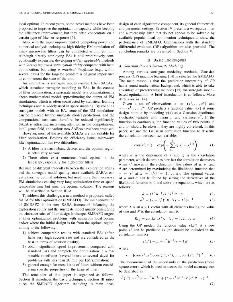
The SMEAFO algorithm is an SAEA. Integrating a surro-gate model into global optimization is much more difficultthan integrating it into space mapping because there is noinformation of the optimal region. Recall the two majordifficulties for filter optimization described in Section I (anillustrative figure is Fig. 1): 1) the optimal region is locatedin a (very) narrow valley of the design space and 2) there areoften numerous local optima. The SAEA, therefore, shouldhave sufficient exploration ability to jump out of local optimain the outer region so as to find the narrow valley and to jumpout of local optima within it. Although this is often achievablefor a modern standard EA, SAEAs may not have the sameexploration ability due to the surrogate model predictionuncertainty, i.e., some optimal designs may be predicted wrongand then the SAEA search is guided to wrong directions.


High exploration ability indicates getting access to diversecandidate designs. To make a good prediction of them, moretraining data points through EM simulations are necessaryto maintain the surrogate model quality, which decreasesthe efficiency. Finding an appropriate balance between theexploration ability and the efficiency for filter design landscapeis the main challenge of SMEAFO.

The required exploration ability in the filter optimizationprocess is different from time to time. Instead of using a fixedSAEA with a certain exploration ability, it is natural to divide itinto the exploration phase aiming to find a near optimal regionand the exploitation phase aiming to obtain the final optimaldesign from near-optimal designs. The latter phase requiresless exploration ability (indicating more space for efficiency)without sacrificing the solution quality. Various methods canbe used for the exploitation phase, and space mapping iscompatible. Because space mapping is sometimes sensitive tothe surrogate model type and settings [7], a surrogate model-assisted Gaussian local search method is used in SMEAFOfor the sake of generality. Now the major challenge is theexploration phase providing both sufficient exploration abilityand efficiency.

To balance the exploration ability and the efficiency,available SAEAs can be mainly classified into “conservative”SAEAs and “active” SAEAs. Conservative SAEAs [22], [23]emphasize the exploration ability. These methods begin witha standard EA for certain iterations aiming to collect trainingdata points that are able to build a reasonably good globalsurrogate model and then iteratively improve the solutionquality and the surrogate model quality in the consecutivesearch. Thus, the exploration ability can benefit a lot atthe cost of a considerable computing overhead for standardEA-based iterations. When applied to filter optimization, muchof this computing overhead is wasted because they are collect-ing training data points for modeling the outer region insteadof the narrow valley where the optimal design is located.

Active SAEAs, in contrast, emphasize the efficiency [15].These methods perform exact expensive evaluations to the“optimal” solutions predicted by the existing surrogate model,despite that its quality may not be good enough. The numberof expensive exact evaluations is therefore highly reduced,but the exploration ability becomes a weakness. Prescreeningmethods [16], [24] are used to assist jumping out of localoptima, but they cannot fully solve the problem. In [15], testson the Ackley benchmark problem (with a narrow valley andmany local optima) [21] (Fig. 1) show that such SAEAs arenot able to jump out of local optima. Hence, the explorationability is insufficient for filter optimization.

The exploration phase of SMEAFO follows the ideaof active SAEAs to avoid consuming considerable EMsimulations to nonoptimal regions. To largely improve theexploration ability compared with existing active SAEAs,two questions are focused: 1) what is the search methodto obtain sufficient exploration ability? and 2) how to buildsurrogate models of sufficient quality using as few samplesas possible (for the sake of efficiency) in order to support theexploration ability? This is achieved by the combination ofa novel surrogate model assisted search method with specific

Fig. 2. Flow diagram of the exploration phase.

DE mutation and training sample selection methods, whichwill be detailed in Section III-B.

B. Design of the Exploration Phase

The general framework of the exploration phase is shownin Fig. 2, which consists of the following steps.

Step 1: Sample λ (often small) candidate designs, performEM simulations of all of them, and let them formthe initial database.

Step 2: Select the λ best designs from the database based onthe objective function values to form a population P .

Step 3: Apply the DE/current-to-best/1 mutation (11) and thecrossover operator (12) on P to generate λ childsolutions.

Step 4: For each child solution, select training data pointsand construct a local GP surrogate model.

Step 5: Prescreen the λ child solutions generated in Step 3using the lower confidence bound method. Estimatethe best child solution based on the lower confidencebound values.

Step 6: Perform EM simulation to the estimated best childsolution from Step 5. Add this design and its per-formance (EM simulation result) to the database.Go back to Step 2 until switching to the exploitationphase.

A main difference compared with available active SAEAsis that a standard EA process is not adopted; instead, only thepredicted best candidate design is simulated and the currentbest λ candidate designs are used as the new population in eachiteration. This new SAEA framework improves the locationsof training data points. It is well known that the number oftraining data points affects the quality of the surrogate model,while their locations are often overlooked. With the samenumber of training data points, it is intuitive that using trainingdata points located near the points waiting to be predicted(child population in Step 3) can obtain surrogate model(s) withbetter quality. This is implemented in Steps 2–6.


From Step 2 to Step 6, in each iteration, the λ currentbest candidate solutions construct the parent population (it isreasonable to assume that the search focuses on the promisingregion) and the best candidate design based on prescreeningin the child population is selected to replace the worst onein the parent population. Hence, only at most one candidateis changed in the parent population in each iteration, so thebest candidate in the child solutions in several consecutiveiterations may not be far from each other (they will then besimulated and are used as training data points). Therefore, thetraining data points describing the current promising regioncan be much denser compared with those generated by astandard EA population updating mechanism, which mayspread in different regions of the design space, while theremay not be sufficient training data points around the candidatesolutions to be prescreened.

Using the database with improved sample locations forsurrogate modeling, a consecutive critical problem is selectingsamples from it which will be used as the training data points.Most SAEAs build a single surrogate model for predicting thechild population. For example, a certain number of evaluatedpromising solutions (ranked by fitness function values) [15]or latest solutions are used to build a model for the childpopulation. But such methods are not suitable for the targetedproblem because of the two design landscape characteristicsof microwave filters (Section III-A). In particular, due to thenarrow valley where the optimal design is located, a promisingpoint that is located near it may be predicted to be notpromising when many training data points are in the outernonoptimal region. The reason is that the hyperparametersin (1) are highly likely to be poorly estimated in likelihoodfunction optimization when the number of training data pointsnear it is insufficient. Therefore, in SMEAFO, a local GPsurrogate model is built for each child solution using τ nearestsamples (based on Euclidean distance). This means that λseparate local GP models are built in each iteration.

With improved surrogate model quality, appropriate searchoperators should be selected to provide neither insufficient norexcessive population diversity, which directly determine theexploration ability. Intuitively, DE/best/1 (9) may not havesufficient population diversity, because the added diversityinto the current best design is not large. Note that althoughthere exist SAEAs with DE/best/1 showing success [25], theoptima of the test problems are not located in a narrowvalley. In contrast, DE/rand/1 (10) may introduce too muchpopulation diversity. DE/current-to-best/1 (11) is in the middle.Pilot experiments on the Ackley benchmark problem [21] arecarried out. Results show that DE/current-to-best/1 just getsan appropriate balance of the population diversity and thesurrogate model quality (almost 100% getting very near tothe global optimum) with the new GP model-assisted searchframework, while DE/rand/1 performs the worst becauseexcessive diversity suffers the surrogate model quality.

It has to be noted that the above particular surrogatemodel-assisted search method, the training data selectionmethod for GP modeling (building a separate GP modelfor each child solution), and the above DE mutationoperator (DE/current-to-best/1) must be used together.

Fig. 3. Flow diagram of the exploitation phase.

Pilot experiments on real-world filters show that when anyof the factors is altered, the algorithm often fails to find thenarrow valley or the performance becomes unstable.

Note that the lower confidence bound method also con-tributes to the algorithm performance. In Step 5, instead of thepredicted value of the GP model, the lower confidence boundvalue (8) is used for ranking. The use of lower confidencebound can balance the search between present promisingregions [i.e., with low y(x) values in (8)] and less exploredregions [i.e., with high s(x) values], so as to improve theability of an SAEA to jump out of local optima. Reference [15]provides more details.

For initial population generation (Step 1), each candidatesolution is calculated by (14) if an initial design is available;otherwise, it is generated randomly within the design space

x j = x initj + N(0, σinit), j = 1, 2, . . . , d (14)

where x init is the initial design and σinit is the standarddeviation of the added Gaussian distributed random number.The value of σinit is roughly estimated according to theresponse of the initial design. Pilot experiments show that theinitial population is far from optimal no matter if using (14)or random generation due to the landscape characteristics ofmicrowave filters and the quality of the initial designs. Notethat SMEAFO performs global optimization and a poor initialpopulation is not a problem and is even assumed.

C. Design of the Exploitation Phase

The general framework of the exploitation phase is shownin Fig. 3, which consists of the following steps.

Step 1: Perform Gaussian local search from the current bestdesign in the database to generate d (number ofdesign variables) solutions.

Step 2: For each solution from Step 1, select training datapoints using the method in Section III-B and con-struct a local GP surrogate model.

Step 3: Prescreen the d solutions generated in Step 1 usingthe lower confidence bound method. For eachof them, if the lower confidence bound value isbetter than the current best design, perform an


EM simulation to it. Add this design and its perfor-mance (the EM simulation result) to the database.

Step 4: If a preset stopping criterion (e.g., computingbudget) is met, output the best solution from thedatabase; otherwise, go back to Step 1.

The goal of the exploitation phase is to obtain the final opti-mal design from a near optimal design based on a surrogate-based local search method with largely reduced explorationability. Although heuristic local search methods themselves arenot complex, a common challenge is the adaptation of criticalparameters, including the starting condition and the scale ofexploitation [26].

Note that there is no clear threshold to divide explorationand exploitation in a search process because “near optimal”is an empirical definition [26]. However, an appropriate def-inition of the starting condition of the exploitation phase isimportant for SMEAFO. Early starting of this phase may makethe algorithm trapped in a local optimum, while late startingdecreases the efficiency. In SMEAFO, we use the averagestandard deviation of the current population P , σP , to reflectthe population diversity or progress of SMEAFO. Often, thevalue of σP first increases (exploring the design space) andthen decreases (converge to the optimal area) in an SMEAFOrun. We set 10% of the maximum σP in the exploration phaseas the threshold to start the exploitation phase.

For the sake of generality, a verified effective method forelaborate search, Gaussian local search (Section II-C), is usedin this phase. σgls is a critical parameter of Gaussian localsearch and is problem dependent. However, with the help ofthe exploration phase, it is set self-adaptively as

σglsj = 0.5 × std(PB j ), j = 1, 2, . . . , d (15)

where P B is the best d candidate designs in the databaseand std is the standard deviation. This indicates that 95.4%(2σ value) of the candidate designs generated by Gaussianlocal search are within the standard deviation of the best davailable candidate designs, which are already in a smallregion. This is in line with the basic idea of this phase(performing local exploitation around the current best design).With the update of P B , the σ gls is self-adapted. Experimentson mathematical benchmark problems and eight real-worldfilter design problems verified empirical settings of σP andthe self-adaptive setting of σ gls.

Considering the surrogate model quality, because this phaseperforms local search, the database provided by the explo-ration phase is a good starting pool of training data points.The training data pool is also updated adaptively by Step 3supporting the consecutive local search. The lower confidencebound value is used in Step 3 to avoid missing potentiallyoptimal solutions, which also provides more samples aroundthe optimal region.

D. Parameter Settings

Besides the self-adaptive parameters and the thresholdvalue to start the exploitation phase (they are no longerparameters), remaining parameters are the DE parameters (λ,F , and CR), the number of training data points (τ ) for each

solution waiting to be prescreened (Step 4 in the explorationphase and Step 2 in the exploitation phase), and σinit (Step 1in the exploration phase).

The DE parameters have clear setting rules. Following [18],we suggest F = 0.8, CR = 0.8, and λ = 50. We suggestτ = 8×d . This is based on the empirical rule in [24] and [25]for online surrogate modeling, and pilot experiments show asuccess. Note that in all the test problems, the same set ofthe above parameters is used. σinit is a rough estimation of thescale to be added to the initial design if it exists. If the responseof the initial design is far from anticipated, a larger σinit canbe used; otherwise, a smaller one may be used. This parameteris not sensitive for most filter design cases because no optimalsolution is expected in the initial population. For some verychallenging cases, using a smaller value is recommended toprevent the valley from becoming too narrow, so as to improvethe solution quality and efficiency. The use of (14) is becauseusing information from the initial design (although may havelow quality) is better than random initialization.

IV. EXPERIMENTAL RESULTS AND COMPARISONS

SMEAFO has been tested by eight real-world filter designproblems (five waveguide filters, one hairpin filter, onemicrostrip filter, and one diplexer). The initial designs areobtained by equivalent circuits or coupling matrix fitting [27].The number of design variables varies from 5 to 22. Thenumber of orders varies from 3 to 16. SMEAFO obtains high-quality results to all of them taking from 10 h to four days.We have not successfully solved six out of eight problems bypopular local optimization-based methods.

In this section, two examples are used to demonstrateSMEAFO for different kinds of filter optimization problemswith different challenges. The first one is a waveguide filter,and the initial design is obtained by coupling matrix fitting.Unfortunately, the initial response is far from the designspecifications. The second one is a microstrip filter. Theinitial design is obtained by an equivalent circuit optimization,and the initial response is reasonably good. However, thisseemingly easy problem is, in fact, difficult because the designlandscape is very rugged, making local search methods fail tojump out of local optima in the narrow valley.

For the first example, ten runs of SMEAFO with indepen-dent random numbers (including initialization) are carried outto test the robustness of SMEAFO and the results are analyzedstatistically. A comparison with standard DE is also carriedout. Because the advantages of the DE algorithm comparedwith some other popular EAs (e.g., genetic algorithm andparticle swarm optimization) in microwave engineering havebeen demonstrated in [28], such comparisons will not berepeated here. For the second example, only a single runof SMEAFO is carried out because standard DE is notaffordable in terms of the computing overhead. The abilityto handle larger search space is especially interesting forfilter optimization because this is a major challenge of filterlandscapes (Section I). This example has 12 design variables,which is relatively large for filter optimization, and we furtherintentionally expand the search ranges of each design variable


Fig. 4. Waveguide filter: T1, input test port, T2: output test port, andR1–R4: resonators.

TABLE I

RANGES OF THE SIX DESIGN VARIABLES (ALL SIZESIN MILLIMETERS) FOR EXAMPLE 1

to make the optimal valley even narrower, so as to verify thecapability of SMEAFO on an extreme case.

Both examples are constrained optimization problems. Thepenalty function method [29] is used to handle the constraints,and the penalty coefficient is set to 50. The examples arerun on a PC with Intel 3.5-GHz Core i7 CPU and 8-GBRAM under Windows operating system. CST is used as theEM simulator. No parallel computation is applied in theseexperiments. All the time consumptions in the experimentsare clock time.

A. Example 1

The first example is a WR-3 band (220–325 GHz)waveguide filter, which is composed of four coupled resonatorsoperating in the TE101 mode. The filter has a Chebyshevresponse [30] (Fig. 4). Because of the fabrication methods inthis frequency range, the filters can be complex in constructionand difficult to design. The ranges of design variables are inTable I. The design specifications are that the passband is from296 to 304 GHz (8-GHz passband centered at 300 GHz) andthe max(|S11|) within the passband should be at least lessthan −20 dB and is as smaller as possible. The stopbandsare from 280 to 292 GHz and from 308 to 320 GHz, wherethe max(|S11|) should be better than −1 dB. Therefore, theoptimization problem is formulated as

minimize max(|S11|), 296 GHz–304 GHz

s.t. min(|S11|) ≥ −1dB, 280 GHz–292 GHz

min(|S11|) ≥ −1dB, 308 GHz–320 GHz. (16)

The initial design is obtained by coupling matrix fitting andis shown in Table II with a performance in Fig. 5(a). It can

TABLE II

INITIAL SOLUTION AND AN OPTIMIZED SOLUTION(ALL SIZES IN MILLIMETERS) FOR EXAMPLE 1

Fig. 5. Response of the waveguide filter.

TABLE III

OPTIMIZED RESULTS USING DIFFERENT METHODS FOR EXAMPLE 1

be seen that this response is far from the specifications. TheNelder–Mead simplex method [5] and the sequential quadraticprogramming method [4] are first used. These two methodsare well-known local optimization methods, and many spacemapping techniques are based on these two search engines.The implementation is based on MATLAB optimization tool-box functions fminsearch and fminimax. Each EM simulationcosts about 2 min. The results are shown in Table III. It canbe seen that both of them fail to find the narrow valley wherethe optimal design is located. It is not a surprise becausethe poor response of the initial design indicates that it is notnear the optimal region, which is a major challenge for localoptimization methods when facing filter design landscapes.

Ten runs with independent random numbers (including tendifferent initial populations) are carried out for SMEAFO todemonstrate the performance and the robustness. Because theinitial response is far from the specifications and consideringthe ranges of the design variables, we set σinit to 0.1. Whenthe generated values by (14) are not within the ranges of thedesign variables, they are set to the nearest bound. As wassaid in Section III-D, the value of σinit is a rough estimation


Fig. 6. SMEAFO convergence trend for Example 1 (average of ten runs).

Fig. 7. DE convergence trend for Example 1.

and is not sensitive. The computing budget is 1000 EMsimulations, but in most runs, convergence happens before800 EM simulations. In all the ten runs using SMEAFO,the constraints are satisfied and the average objective functionvalue is −24.14 dB. The best value is −26.90 dB, the worstvalue is −17.72 dB, and the standard deviation is 3.37.Eight out of ten runs obtain max(|S11|) (296–304 GHz) smallerthan −24 dB. A medium one is provided in Tables II (opti-mized design variables) and III and Fig. 5(b) (performance).The convergence trend is shown in Fig. 6. It can be seenthat the design quality is satisfactory using less than 600 EMsimulations on average.

DE is also carried out using the initial population of theSMEAFO run provided in Tables II and III with the samerelated algorithm parameters of SMEAFO. The computingbudget is set to 25 000 EM simulations. The obtained resultis −22.86 dB. Hence, SMEAFO obtains more than 33 timesspeed improvement compared with standard DE for this exam-ple, making the unbearable time to be very practical (onemonth to one day) and obtaining an even better result. Theconvergence trend of DE is shown in Fig. 7. Comparing thetwo convergence trends, some observations can be made.

On average, the exploitation phase of SMEAFO starts fromabout 540 EM simulations with the starting performanceof about −17 dB (according to the rule defined inSection III-C). The observations are as follows.

1) DE completes the exploration using about 8500 EMsimulations (obtaining −17 dB), while SMEAFO uses

Fig. 8. Microstrip filter: front view.

TABLE IV

RANGES OF THE 12 DESIGN VARIABLES (ALL SIZES

IN MILLIMETERS) FOR EXAMPLE 2

about 540 EM simulations, obtaining about 16 timesspeed improvement.

2) DE then costs 16 500 EM simulations to improve theresult from near-optimal designs to the final optimizeddesign because of the rugged landscape in the val-ley, while the exploitation phase of SMEAFO costsabout 250 EM simulations to get a better solution,achieving about 66 times speed improvement. This veri-fies the effectiveness of main ideas of SMEAFO in bothphases.

B. Example 2

The second example is an eighth-order microstrip filterworking from 3.3 to 7.3 GHz, which is shown in Fig. 8.The ranges of design variables are in Table IV. As mentionedabove, they are intentionally expanded to test SMEAFO inan extreme condition. The design specifications are that thepassband is from 4 to 7 GHz and the stopbands are from3.3 to 3.92 GHz and from 7.08 to 7.3 GHz. Therefore, theoptimization problem is defined as follows:

minimize max(|S11|), 4 GHz–7 GHz

s.t. min(|S11|) ≥ −3dB, 3.3 GHz–3.92 GHz

min(|S11|) ≥ −3dB, 7.08 GHz–7.3 GHz. (17)

An equivalent circuit model is available, which is usedfor a first optimization to get the initial design, in whichthe simulation is performed by ADS circuit simulator (notMomentum). Because each ADS circuit simulation only costsa few seconds, standard DE is used. The optimized designvariables (initial design for full-wave optimization) are shownin Table V with a performance in Fig. 9(a). It can be seenthat the response of the optimized design using the equivalentcircuit model is excellent in terms of circuit simulation, andwhen simulating it with the full-wave EM model, the responseseems to be good as a starting point and only a slight movefrom the initial design is needed. However, this “correct slightmove” is difficult.


TABLE V

INITIAL SOLUTION AND AN OPTIMIZED SOLUTION(ALL SIZES IN MILLIMETERS) FOR EXAMPLE 2

Fig. 9. Response of the microstrip filter.

TABLE VI

OPTIMIZED RESULTS USING DIFFERENT METHODS FOR EXAMPLE 2

The Nelder–Mead simplex method and the sequentialquadratic programming method are first applied. Note thatthese local optimization methods are not affected by theexpanded search ranges, as a good starting point is available.For this example, each EM simulation costs about 3–6 min.The results are shown in Table VI. It can be seen thatNelder–Mead simplex fails to jump out of local optima,although the initial design is near the narrow valley, whilesequential quadratic programming goes out of the narrowvalley and is trapped in a local optimum in the outer region.Simulation data indicates that in all the eight test problems,this problem has the most rugged landscape.

Then, SMEAFO is carried out. Because of the intentionallyset large ranges of the design variables, σinit is set to 0.25. Aswas said in Section III-D, the value of σinit is a rough estima-tion and is not sensitive. The computing budget is 1250 EMsimulations. The results are shown in Tables V (optimizeddesign variables) and VI and Fig. 9(b) (performance). Theconvergence trend is shown in Fig. 10. It can be seen thatSMEAFO obtains a satisfactory result for this very challengingproblem in terms of the ruggedness of the landscape and the

Fig. 10. SMEAFO convergence trend for Example 2.

narrowness of the optimal valley. This example shows that forproblems that space mapping seems to be the suitable method,there are exceptions and SMEAFO can be a supplement forthese exceptions.

Experiments on our real-world filter design test cases showthat most hard filter optimization can be finished within700 EM simulations using SMEAFO obtaining satisfactoryresults. For most test cases, the optimization time is one totwo days. Note that SMEAFO is designed for filter opti-mization problems that may be difficult to solve by existinglocal optimization methods (space mapping-based methodswithout problem specific tuning often at most obtain the samesolution quality compared with direct local search), comparingspeed with such methods is therefore not relevant. Rather, anexcellent result in a reasonable timeframe for hard problemsis the goal of SMEAFO.

V. CONCLUSION

In this paper, the SMEAFO algorithm has been pro-posed. SMEAFO is aimed to serve as a widely applicablemethod (i.e., not restricted by filter types/responses) targetedat microwave filter optimization problems that are difficult tobe solved by popular local optimization methods, while at thesame time are not affordable to be solved by standard globaloptimization methods, so as to complement the state of thearts. Experiments show that SMEAFO can provide optimalfilter designs that are comparable with the DE algorithm,which is expected to provide very high-quality design, but usesa reasonable timeframe and is several orders faster than DE.These results are achieved by our novel SAEA designed forfilter landscapes, including the two-phase structure, the novelsurrogate model-assisted search methods, and the training dataselection method in each phase. In addition, SMEAFO witha lower fidelity EM model can be used to support spacemapping, providing a good initial design and a databasewith lower fidelity model evaluation results. The SMEAFO-based filter design optimization tool can be downloaded fromhttp://fde.cadescenter.com. Future works include developingparallelized SMEAFO.

ACKNOWLEDGMENT

The authors would like to thank Prof. S. Koziel, ReykjavikUniversity, Iceland, for valuable discussions.


REFERENCES

[1] M. Fakhfakh, E. Tlelo-Cuautle, and P. Siarry, Computational Intelligencein Analog and Mixed-Signal (AMS) and Radio-Frequency (RF) CircuitDesign. Berlin, Germany: Springer, 2015.

[2] A. Deb, J. S. Roy, and B. Gupta, “Performance comparison of dif-ferential evolution, particle swarm optimization and genetic algorithmin the design of circularly polarized microstrip antennas,” IEEE Trans.Antennas Propag., vol. 62, no. 8, pp. 3920–3928, Aug. 2014.

[3] N. He, D. Xu, and L. Huang, “The application of particle swarmoptimization to passive and hybrid active power filter design,” IEEETrans. Ind. Electron., vol. 56, no. 8, pp. 2841–2851, Aug. 2009.

[4] P. T. Boggs and J. W. Tolle, “Sequential quadratic programming,” ActaNumer., vol. 4, pp. 1–51, Jan. 1995.

[5] J. C. Lagarias, J. A. Reeds, M. H. Wright, and P. E. Wright, “Conver-gence properties of the Nelder–Mead simplex method in low dimen-sions,” SIAM J. Optim., vol. 9, no. 1, pp. 112–147, 1998.

[6] M. Sans, J. Selga, A. Rodríguez, J. Bonache, V. E. Boria, and F. Martín,“Design of planar wideband bandpass filters from specifications usinga two-step aggressive space mapping (ASM) optimization algorithm,”IEEE Trans. Microw. Theory Techn., vol. 62, no. 12, pp. 3341–3350,Dec. 2014.

[7] S. Koziel, S. Ogurtsov, J. W. Bandler, and Q. S. Cheng, “Reliable space-mapping optimization integrated with EM-based adjoint sensitivities,”IEEE Trans. Microw. Theory Techn., vol. 61, no. 10, pp. 3493–3502,Oct. 2013.

[8] X. Shang, Y. Wang, G. L. Nicholson, and M. J. Lancaster, “Designof multiple-passband filters using coupling matrix optimisation,” IETMicrow., Antennas Propag., vol. 6, no. 1, pp. 24–30, 2012.

[9] J. W. Bandler, R. M. Biernacki, S. H. Chen, P. A. Grobelny, andR. H. Hemmers, “Space mapping technique for electromagnetic opti-mization,” IEEE Trans. Microw. Theory Techn., vol. 42, no. 12,pp. 2536–2544, Dec. 1994.

[10] C. Zhang, F. Feng, V.-M.-R. Gongal-Reddy, Q. J. Zhang, andJ. W. Bandler, “Cognition-driven formulation of space mapping forequal-ripple optimization of microwave filters,” IEEE Trans. Microw.Theory Techn., vol. 63, no. 7, pp. 2154–2165, Jul. 2015.

[11] Q. S. Cheng, J. W. Bandler, and S. Koziel, “Space mapping designframework exploiting tuning elements,” IEEE Trans. Microw. TheoryTechn., vol. 58, no. 1, pp. 136–144, Jan. 2010.

[12] R. Ben Ayed, J. Gong, S. Brisset, F. Gillon, and P. Brochet, “Three-leveloutput space mapping strategy for electromagnetic design optimization,”IEEE Trans. Magn., vol. 48, no. 2, pp. 671–674, Feb. 2012.

[13] M. A. E. Sabbagh, M. H. Bakr, and J. W. Bandler, “Adjoint higher ordersensitivities for fast full-wave optimization of microwave filters,” IEEETrans. Microw. Theory Techn., vol. 54, no. 8, pp. 3339–3351, Aug. 2006.

[14] T. J. Santner, B. J. Williams, and W. I. Notz, The Design and Analysisof Computer Experiments. Berlin, Germany: Springer, 2013.

[15] M. T. M. Emmerich, K. C. Giannakoglou, and B. Naujoks, “Single-and multiobjective evolutionary optimization assisted by Gaussian ran-dom field metamodels,” IEEE Trans. Evol. Comput., vol. 10, no. 4,pp. 421–439, Aug. 2006.

[16] J. E. Dennis and V. Torczon, “Managing approximation models inoptimization,” in Multidisciplinary Design Optimization: State of theArt. Hampton, VA, USA: SIAM, 1997, pp. 330–347.

[17] I. Couckuyt, A. Forrester, D. Gorissen, F. De Turck, and T. Dhaene,“Blind Kriging: Implementation and performance analysis,” Adv. Eng.Softw., vol. 49, pp. 1–13, Jul. 2012.

[18] K. Price, R. M. Storn, and J. A. Lampinen, Differential Evolution:A Practical Approach to Global Optimization. New York, NY, USA:Springer-Verlag, 2005.

[19] A. Hoorfar, “Evolutionary programming in electromagnetic optimiza-tion: A review,” IEEE Trans. Antennas Propag., vol. 55, no. 3,pp. 523–537, Mar. 2007.

[20] X. Yao, Y. Liu, and G. Lin, “Evolutionary programming made faster,”IEEE Trans. Evol. Comput., vol. 3, no. 2, pp. 82–102, Jul. 1999.

[21] M. Jamil and X.-S. Yang, “A literature survey of benchmark functionsfor global optimisation problems,” Int. J. Math. Model. Numer. Optim.,vol. 4, no. 2, pp. 150–194, 2013.

[22] D. Lim, Y. Jin, Y. S. Ong, and B. Sendhoff, “Generalizing surrogate-assisted evolutionary computation,” IEEE Trans. Evol. Comput., vol. 14,no. 3, pp. 329–355, Jun. 2010.

[23] Z. Zhou, Y. S. Ong, P. B. Nair, A. J. Keane, and K. Y. Lum, “Combiningglobal and local surrogate models to accelerate evolutionary optimiza-tion,” IEEE Trans. Syst., Man, Cybern. C, Appl. Rev., vol. 37, no. 1,pp. 66–76, Jan. 2007.

[24] D. R. Jones, M. Schonlau, and W. J. Welch, “Efficient global optimiza-tion of expensive black-box functions,” J. Global Optim., vol. 13, no. 4,pp. 455–492, 1998.

[25] B. Liu, D. Zhao, P. Reynaert, and G. G. E. Gielen, “Synthesis ofintegrated passive components for high-frequency RF ICs based onevolutionary computation and machine learning techniques,” IEEETrans. Comput.-Aided Des. Integr. Circuits Syst., vol. 30, no. 10,pp. 1458–1468, Oct. 2011.

[26] C. C. Coello, G. B. Lamont, and D. A. Van Veldhuizen, EvolutionaryAlgorithms for Solving Multi-Objective Problems. Springer, 2007.

[27] J.-S. G. Hong and M. J. Lancaster, Microstrip Filters for RF/MicrowaveApplications, vol. 167. Hoboken, NJ, USA: Wiley, 2004.

[28] P. Rocca, G. Oliveri, and A. Massa, “Differential evolution as appliedto electromagnetics,” IEEE Antennas Propag. Mag., vol. 53, no. 1,pp. 38–49, Feb. 2011.

[29] D. M. Himmelblau, Applied Nonlinear Programming. New York, NY,USA: McGraw-Hill, 1972.

[30] X. Shang, M. Ke, Y. Wang, and M. J. Lancaster, “WR-3 bandwaveguides and filters fabricated using SU8 photoresist micromachiningtechnology,” IEEE Trans. THz Sci. Technol., vol. 2, no. 6, pp. 629–637,Nov. 2012.

Bo Liu (M’15) received the B.S. degree fromTsinghua University, Beijing, China, in 2008, andthe Ph.D. degree from MICAS Laboratories, Uni-versity of Leuven, Leuven, Belgium, in 2012.

From 2012 to 2013, he was a Humboldt ResearchFellow with the Technical University of Dortmund,Dortmund, Germany. In 2013, he joined WrexhamGlyndwr University, Wrexham, U.K., as a Lecturer,where he became a Reader of computer-aided designin 2016. He is currently an Honorary Fellow with theUniversity of Birmingham, Edgbaston, Birmingham,

U.K. He has authored or co-authored 1 book and more than 40 papers ininternational journals, edited books, and conference proceedings. His currentresearch interests include design automation methodologies of analog/RFintegrated circuits, microwave devices, MEMS, evolutionary computation, andmachine learning.

Hao Yang was born in Wuhan, China, in 1991.He received the B.Eng. degree in electronics andinformation engineering from the Huazhong Univer-sity of Science and Technology, Wuhan, in 2014,and the B.Eng. degree in electronic and electricalengineering from the University of Birmingham,Edgbaston, Birmingham, U.K., in 2014, where heis currently pursuing the Ph.D. degree.

His current research interests include terahertzfrequency filters and mutiplexers.

Michael J. Lancaster (SM’04) was born in WestYorkshire, U.K., in 1958. He received the bachelor’sdegree in physics and Ph.D. degree (with a focus onnonlinear underwater acoustics) from the Universityof Bath, Bath, U.K., in 1980 and 1984, respectively.

He was a Research Fellow with the SurfaceAcoustic Wave (SAW) Group, Department ofEngineering Science, Oxford University, Oxford,U.K., where he was involved in the design ofnew, novel SAW devices, including RF filters andfilter banks. In 1987, he became a Lecturer in

electromagnetic theory and microwave engineering with the Department ofElectronic and Electrical Engineering, University of Birmingham, Edgbaston,Birmingham, U.K., where he was involved in the study of the science andapplications of high-temperature superconductors, mainly at microwavefrequencies, and became the Head of the Department of Electronic, Electrical,and Systems Engineering in 2003. He has authored 2 books and over 190papers in refereed journals. His current research interests include microwavefilters and antennas, high-frequency properties and applications of a numberof novel and diverse materials, and micromachining as applied to terahertzcommunications devices and systems.

Prof. Lancaster is a Fellow of the IET and the Institute of Physics, U.K.He is a Chartered Engineer and a Chartered Physicist. He has served on theIEEE MTT-S IMS Technical Committees.

1976 ieee transactions on microwave theory and …

Documents