2016 depreciation study
TRANSCRIPT

2016 DEPRECIATION STUDY
CALCULATED ANNUAL DEPRECIATION ACCRUALS RELATED TO WATER PLANT
AS OF DECEMBER 31, 2016
Prepared by:

NEW JERSEY AMERICAN WATER COMPANY Voorhees, New Jersey
2016 DEPRECIATION STUDY
CALCULATED ANNUAL DEPRECIATION
ACCRUALS RELATED TO WATER PLANT
AS OF DECEMBER 31, 2016
GANNETT FLEMING VALUATION AND RATE CONSULTANTS, LLC
Camp Hill, Pennsylvania


TABLE OF CONTENTS
EXECUTIVE SUMMARY . . . . . . . . . . . . . . . . . . .. . ... . . . . . . . . . . . .. . . . . . . . . . . .... .. . . .. . . . . . . . . . . . . . . . . . . . . . . ........ iii
PART I. INTRODUCTION...................................................................................... 1-1 Scope .................................................................................................................... 1-2 Plan of Report . . . . . . . . . . . . . . . . . . . . . . . . . . . . . . . . . . . . . . . . . . . . . . . . . . . . . . . . . . . . . . . . . . . . . . . . . . . . . . . . . . . . . . . . . . . . . . . . . . . . . . . . 1-2 Basis of the Study . . . . . . . . . . . . . . . . . . . . . . . . . . . . . . . . . . . . . . . . . . . . . . . . . . . . . . . . . . . . . . . . . . . . . . . . . . . . . . . . . . . . . . . . . . . . . . . . . . 1-3
Depreciation ................................................................................................ 1-3 Service Life Estimates and Net Salvage Normalization............................... 1-4
PART II. ESTIMATION OF SURVIVOR CURVES................................................. 11-1 Survivor Curves...................................................................................................... 11-2
Iowa Type Curves........................................................................................ 11-3 Retirement Rate Method of Analysis........................................................... 11-9 Schedules of Annual Transactions in Plant Records................................... 11-10 Schedule of Plant Exposed to Retirement................................................... 11-13 Original Life Table ...................................................................................... 11-15 Smoothing the Original Survivor Curve........................................................ 11-17
PART Ill. SERVICE LIFE CONSIDERATIONS..................................................... 111-1 Field Trips.............................................................................................................. 111-2 Service Life Analysis.............................................................................................. 111-2
PART IV. NET SALVAGE CONSIDERATIONS................................................... IV-1 Net Salvage Normalization..................................................................................... IV-2
PART V. CALCULATION OF ANNUAL AND ACCRUED DEPRECIATION......... V-1 Group Depreciation Procedures............................................................................. V-2
Single Unit of Property................................................................................. V-2 Group Depreciation Procedures.................................................................. V-3 Remaining Life Annual Accruals.................................................................. V-3 Average Service Life Procedure.................................................................. V-3
Calculation of Annual and Accrued Amortization.................................................... V-4
PART VI. RESULTS OF STUDY.......................................................................... Vl-1 Qualification of Results........................................................................................... Vl-2 Description of Detailed Tabulations........................................................................ Vl-2
~ 6annett Fleming New Jersey American Water Co - Water December 31, 2016

TABLE OF CONTENTS, cont.
Table 1. Summary of Estimated Survivor Curves, Original Cost, Book Depreciation Reserve, and Calculated Annual Depreciation Accrual Rates and Net Salvage Normalization as of December 31, 2016........ Vl-4
Table 2. Calculation of Net Salvage Normalization........................................... Vl-7
PART VII. SERVICE LIFE STATISTICS................................................................ Vll-1
PART VIII. DETAILED DEPRECIATION CALCULATIONS .................................. Vllll-1
~ 6annettF/eming ii New Jersey American Water Co - Water December 31, 2016

EXECUTIVE SUMMARY
Pursuant to New Jersey American Water Company's ("NJAWC") request, Gannett
Fleming Valuation and Rate Consultants, LLC ("Gannett Fleming") has conducted a
depreciation study related to NJAWC plant as of December 31, 2016. The purpose of
this study was to determine the annual depreciation accrual rates and amounts for book
and ratemaking purposes.
The depreciation rates are based on the straight line method using the average
service life ("ASL") procedure and were applied on a remaining life basis. The
calculations were based on attained ages and estimated average service life as well as
the net salvage normalization for each depreciable group of assets.
NJAWC's accounting policy has not changed since the previous depreciation study
was prepared, nor were there any significant policy changes that might affect the results
of the study presented here. However, some average service life estimates proposed in
this study have changed from the currently approved estimates. The overall depreciation
accrual rate has increased since the last study was performed.
Gannett Fleming recommends the calculated annual depreciation accrual rates
proposed herein apply specifically to NJAWC's plant in service as of December 31, 2016
as summarized in Table 1 of the study. The study sets forth a total annual depreciation
expense of $123.5 million as applied to the depreciable original cost of $4.38 billion as of
December 31, 2016.
Gannett Fleming iii New Jersey American Water Co - Water December 31, 2016

~ 6annettF/eming 1-1
PART I. INTRODUCTION
New Jersey American Water Co - Water December 31, 2016

NEW JERSEY AMERICAN WATER COMPANY
DEPRECIATION STUDY
PART I. INTRODUCTION
SCOPE
This report presents the results of the depreciation study prepared for the New
Jersey American Water Company as applied to water plant in service as of December 31,
2016. It relates to the concepts, methods, and basic judgments which underlie
recommended annual depreciation accrual rates related to current utility plant in service.
The service life estimates resulting from the study were based on informed
judgment which incorporated analyses of historical plant retirement data as recorded
through 2016; a review of Company practice and outlook as they relate to plant operation
and retirement; and consideration of current practice in the water industry, including
knowledge of service life estimates used for other water properties.
PLAN OF REPORT
Part I, Introduction, contains statements with respect to the plan of the report, and
the basis of the study. Part II, Estimation of Survivor Curves, presents descriptions of the
considerations and the methods used in the service life studies. Part Ill, Service Life
Considerations, presents the factors and judgment utilized in the average service life
analysis. Part IV, Net Salvage Considerations, presents the judgment utilized of the net
salvage study. Part V, Calculation of Annual and Accrued Depreciation, describes the
procedures used in the calculation of group depreciation. Part VI, Results of Study,
presents summaries by depreciable group of annual depreciation accrual rates and
amounts, as well as composite remaining lives. Part VII, Service Life Statistics presents
the statistical analysis of service life estimates, and Part VIII, Detailed Depreciation
Calculations presents the detailed tabulations of annual depreciation.
Gannett Fleming 1-2 New Jersey American Water Co - Water December 31, 2016

BASIS OF THE STUDY
Depreciation
Depreciation, in public utility regulation, is the loss in service value not restored by
current maintenance, incurred in connection with the consumption or prospective
retirement of utility plant in the course of service from causes which are known to be in
current operation and against which the utility is not protected by insurance. Among
causes to be given consideration are wear and tear, deterioration, action of the elements,
inadequacy, obsolescence, changes in the art, changes in demand, and the requirements
of public authorities.
Depreciation, as used in accounting, is a method of distributing fixed capital costs,
less net salvage, over a period of time by allocating annual amounts to expense. Each
annual amount of such depreciation expense is part of that year's total cost of providing
water utility service. Normally, the period of time over which the fixed capital cost is
allocated to the cost of service is equal to the period of time over which an item renders
service, that is, the item's service life. The most prevalent method of allocation is to
distribute an equal amount of cost to each year of service life. This method is known as
the straight-line method of depreciation.
For most accounts, the annual depreciation was calculated by the straight line
method using the average service life procedure and the remaining life basis. For certain
General Plant accounts, the annual depreciation is based on amortization accounting.
Both types of calculations were based on original cost, attained ages, and estimates of
service lives.
The straight line method, average service life procedure is a commonly used
depreciation calculation procedure that has been widely accepted in jurisdictions
throughout North America. Gannett Fleming recommends its continued use. Amortization
accounting is used for certain General Plant accounts because of the disproportionate
~ 6annettF/eming 1-3 New Jersey American Water Co - Water December 31, 2016

plant accounting effort required when compared to the minimal original cost of the large
number of items in these accounts. An explanation of the calculation of annual and
accrued amortization is presented beginning on page V-4 of the report.
Service Life Estimates and Net Salvage Normalization
The service life estimates used in the depreciation and amortization calculations
were based on informed judgment which incorporated a review of management's plans,
policies and outlook, a general knowledge of the water utility industry, and comparisons
of the service life and net salvage estimates from our studies of other water utilities. The
use of survivor curves to reflect the expected dispersion of retirement provides a
consistent method of estimating depreciation for water plant. Iowa type survivor curves
were used to depict the estimated survivor curves for the plant accounts not subject to
amortization accounting.
The procedure for estimating service lives consisted of compiling historical data
for the plant accounts or depreciable groups, analyzing this history through the use of
widely accepted techniques, and forecasting the survivor characteristics for each
depreciable group on the basis of interpretations of the historical data analyses and the
probable future. The combination of the historical experience and the estimated future
yielded estimated survivor curves from which the average service lives were derived.
The estimates of net salvage by account incorporated a review of experienced
costs of removal and salvage related to transactions over the last three years. Each
component of net salvage, i.e. cost of removal and salvage, was stated in dollars incurred
during the three-year period.
An understanding of the function of the plant and information with respect to the
reasons for past retirements and the expected causes of future retirements was obtained
through field trips and discussions with operating and management personnel. The
Gannett Fleming 1-4 New Jersey American Water Co - Water December 31, 2016

supplemental information obtained in this manner was considered in the interpretation
and extrapolation of the statistical analyses.
6annettF/eming 1-5 New Jersey American Water Co - Water December 31, 2016

~ Gannett Fleming 11-1
PART II. ESTIMATION OF SURVIVOR CURVES
New Jersey American Water Co - Water December 31, 2016

PART II. ESTIMATION OF SURVIVOR CURVES
The calculation of annual depreciation based on the straight line method requires
the estimation of survivor curves and the selection of group depreciation procedures. The
estimation of survivor curves is discussed below and the development of net salvage is
discussed in later sections of this report.
SURVIVOR CURVES
The use of an average service life for a property group implies that the various
units in the group have different lives. Thus, the average life may be obtained by
determining the separate lives of each of the units, or by constructing a survivor curve by
plotting the number of units which survive at successive ages.
The survivor curve graphically depicts the amount of property existing at each age
throughout the life of an original group. From the survivor curve, the average life of the
group, the remaining life expectancy, the probable life, and the frequency curve can be
calculated. In Figure 1, a typical smooth survivor curve and the derived curves are
illustrated. The average life is obtained by calculating the area under the survivor curve,
from age zero to the maximum age, and dividing this area by the ordinate at age zero.
The remaining life expectancy at any age can be calculated by obtaining the area under
the curve, from the observation age to the maximum age, and dividing this area by the
percent surviving at the observation age. For example, in Figure 1, the remaining life at
age 30 is equal to the crosshatched area under the survivor curve divided by 29.5 percent
surviving at age 30. The probable life at any age is developed by adding the age and
remaining life. If the probable life of the property is calculated for each year of age, the
probable life curve shown in the chart can be developed. The frequency curve presents
the number of units retired in each age interval. It is derived by obtaining the differences
between the amount of property surviving at the beginning and at the end of each interval.
6annett Fleming 11-2 New Jersey American Water Co - Water December 31, 2016

This study has incorporated the use of Iowa curves developed from a retirement
rate analysis of historical retirement history. A discussion of the concepts of survivor
curves and of the development of survivor curves using the retirement rate method is
presented below.
Iowa Type Curves
The range of survivor characteristics usually experienced by utility and industrial
properties is encompassed by a system of generalized survivor curves known as the Iowa
type curves. There are four families in the Iowa system, labeled in accordance with the
location of the modes of the retirements in relationship to the average life and the relative
height of the modes. The left moded curves, presented in Figure 2, are those in which
the greatest frequency of retirement occurs to the left of, or prior to, average service life.
The symmetrical moded curves, presented in Figure 3, are those in which the greatest
frequency of retirement occurs at average service life. The right moded curves, presented
in Figure 4, are those in which the greatest frequency occurs to the right of, or after,
average service life. The origin moded curves, presented in Figure 5, are those in which
the greatest frequency of retirement occurs at the origin, or immediately after age zero.
The letter designation of each family of curves (L, S, R or 0) represents the location of
the mode of the associated frequency curve with respect to the average service life. The
numbers represent the relative heights of the modes of the frequency curves within each
family.
The Iowa curves were developed at the Iowa State College Engineering
Experiment Station through an extensive process of observation and classification of the
ages at which industrial property had been retired. A report of the study which resulted
in the classification of property survivor characteristics into 18 type curves,
liannett Fleming 11-3 New Jersey American Water Co - Water December 31, 2016

[Bf
en ~ I
10
0
i ~I
90
l! ~
80
...
. I
~ I
70
O>
-~
60
>
>
s..
::,
- ~ .b.
I
(JJ
50
....
-C
~
G)
(J
s.. a>
40
a.
- - -
z 3
0
CD
-::: c:.
.. CD
..., en
~I
)>
20
3 ~ o·
o ~
I 10
~~
CD
DJ
3 -
O'"
~
~
()
(,J
0 ...
.>.
I
~~
0 DJ
.....
. -0
) ~
0
~ "'
\ '\
.....---s
urv
ivo
r C
urv
e
\-L.
.,-P
roba
ble
Life
Cu
rve
~ \
\ \
\ \
Ave
rag
e L
ife
\~
\ '-
~ I
I I
I '-
' M
axi
mu
m L
ife
,
\ \
~
Pro
ba
ble
Lif
e
' \
~
"" -=: ::
xpe
cta
ncy
~
Ag
e
Mod
e \.
~
\ \.
~
~ ~ "'
F
req
ue
ncy
Cu
rve
~ ,,,,
,.------
.... ~
~
/ ~ W
//~
~ ""'-
-~
~
~
'-ij//// ////,,
5 10
15
20
2
5
30
3
5
40
4
5
50
Ag
e I
n Y
ea
rs
Fig
ure
1.
A T
ypic
al S
urv
ivo
r C
urv
e an
d D
eriv
ed C
urv
es
~
55
60
:u ~ :.; a.
4 l
3 ~ c
2 1l :.; a.

~
g, ~ l'D
l"'to
l"'to :tl ~ 5· LC
:i I 01
z ~ c....
(1) iil
(1)
'<
)>
3 (1) £.
0::
J
(1) ~
@ Il
l
3 ro
C""
"'
(1)
()
""'0
~.
~ ::
E O
il>
mm
""'
10
0
--
90
1
~
ao
I I
70
I
I
C>
so I
C
I >
>
L
..
:::,
Cl)
5
0
-C Cl) 0 L..
C
l) 4
0
a..
30
20
10
0 2
5 -
--
-~
50
i:
> ,;;;
: ,. Ii:
: ,. ' "'
" I
I I
i45
~4
0
e ~3
5
0
/ L
5
/u \
r i\\
~ r:,
n
L1
~ ~
I>
..
~/ ~ ~
LO
' r-,.;::
'< ~
' \l
\
\ "
I I
I ::
30
I '
...
.g
,4'.
\I \
\\
j25
I I
e
I ~
\\I
I ~
20
,,:;
I g
15
I C
l :, f1
0
IL
5
0 2
5
50
7
5
10
0
12
5
15
0
17
5
20
0
22
5
25
0
27
5
30
0
Ag
e, P
erc
en
t o
f A
vera
ge
Life
50
7
5
10
0
12
5
15
0
17
5
20
0
22
5
25
0
27
5
30
0
Ag
e,
Pe
rce
nt
of
Ave
rag
e L
ife
Fig
ure
2.
Le
ft M
od
al
or
"L"
Iow
a T
yp
e S
urv
ivo
r C
urv
es

[e
~ 5 rn ~ lJ ~ 5· IQ
I 0)
z ~ c:_
(D
iil ~
)>
3 (D @"
0::
J
~~
(D
Ill
3 ro
CT
-,
(D
(")
-,
0 ~.
~~
mar -,
10
0
90
I
ao I
70
I
C>
ao I
C
: > "> L
..
::::,
(f)
50
-C: Q
) 0 L
..
Q)
40
a..
30
20
10
0
--
--
--
-6
0
.!!
I ""~
''\\\
I I
~ 4
5
-<
~ ~
-..
. I
~ ~ 4
0
• f 35
I
.,
I'<
'<
3\-1>
.t \
\I
11.
I I
I ~ 3
0
~ 2
5
C .,
I I
'-.I
~ .. ,\\
\\ I
I
~ 2
0
I 11
. ~1
5
I I
I I
I ]
I I
S8
I I
J 1
I .
~ L---1
--+--t
----rr
li ,, -
~, -
~
~, s,
1\
I I
1,\\
\\1
.. I
I ~
10
e IL
5
8 S
_
/,,.
s-
'-
/ I
J\,~
"~
I
I J
....
....
..-:
:~r.
.i
"-0
25
5
0
75
1
00
1
25
1
50
1
75
2
00
2
25
2
50
2
75
3
00
Ag
a.
Pe
rce
nt
of
Ave
rag
e L
ife
25
5
0
75
1
00
1
25
1
50
1
75
2
00
2
25
2
50
2
75
3
00
Ag
e,
Pe
rce
nt
of
Ave
rag
e L
ife
Fig
ure
3.
Sym
me
tric
al
or
"S"
Iow
a T
yp
e S
urv
ivo
r C
urv
es

re
&11
10
0
5 l'b
I ,....
9
0
,.... ,, rr
I 8
0
:3 5· lQ I
70
O>
C ·s:
60
-~
:::
:,
C/J
50
-C Q
) (.
)
.!_i I
<ii 4
0
a.
30
20
z (1
) :E
c.... !!l
I 1
0
en
(1)
'<
)>
3 !)l
o~
· 0
(1) ~
£ Q
) 3
.....
O"
!)l
!)l
()
vJ
0 ...
>.
I
N~
0
Q)
........
.. O
l !)l
25
5
0
75
1
00
1
25
1
50
,o5
0
"ii 145
1
:40
~ l35
0 ::
30
.e 1
:25
~ :20
~1
5
:i ::, e1
0 u.
5
~
c:.
- ~ ,/
'/
R6 j\
I ~, ,1 R3
' i/
~
,:,
•'-
-R1
,,..._ _
\.
~ ~ ....
......
0 2
5
50
7
5
10
0
12
5
15
0
17
5
20
0
22
5
25
0
27
5
30
0
Ag
e,
Pe
rce
nt
of
Ave
rag
e L
ife
17
5
20
0
22
5
25
0
27
5
Ag
e,
Pe
rce
nt
of
Ave
rag
e L
ife
Fig
ure
4.
Rig
ht
Mo
da
l o
r "R
" Io
wa
Typ
e S
urv
ivo
r C
urv
es
30
0

en ! I
10
0
:::J
~I
90
""" :ti ~I
80
5· ~I
70
C)
C:
·s;
60
·s;
L
..
::::,
en
50
.....
C
: <
I)
co I
0 L..
4
0
<I)
a..
30
z 2
0
CD
::E
c...
CD
-, ~I
'<
10
)>
3 CD
o~
· 0
25
~ ~
CD
Ill
3 r+
O" ~
~o
w
o
_..
I
-N ~
Olll
....
..
r+
0) ~
50
7
5
10
0
12
5
15
0
•20
! .!
18
.!:
j 1
6
e ~1
4
0 :: 1
2
.g
E1
0
~ ~ 8
r; 6
C " g.
4 I!! IL
2
..
~
04
DI. .....
.. 0
3
~2
I
~
01
' ~
_::
, '
..........
.. L~
,._
1 ....
......
...
L I
o ~ ~
n 10
0 1
~
1~
1
n ~ ~ ~ ~ ~
Ag
e,
Pe
rce
nt
of
Ave
rag
e L
ife
17
5
20
0
22
5
25
0
27
5
Ag
e,
Pe
rce
nt
of
Ave
rag
e L
ife
Fig
ure
5.
Ori
gin
Mo
da
l o
r "O
" Io
wa
Typ
e S
urv
ivo
r C
urv
es
30
0

which constitute three of the four families, was published in 1935 in the form of the
Experiment Station's Bulletin 125. These curve types have also been presented in
subsequent Experiment Station bulletins and in the text, "Engineering Valuation and
Depreciation."1 In 1957, Frank V. B. Couch, Jr., an Iowa State College graduate student
submitted a thesis presenting his development of the fourth family consisting of the four
0 type survivor curves.
Retirement Rate Method of Analysis
The retirement rate method is an actuarial method of deriving survivor curves using
the average rates at which property of each age group is retired. The method relates to
property groups for which aged accounting experience is available and is the method
used to develop the original stub survivor curves in this study. The method (also known
as the annual rate method) is illustrated through the use of an example in the following
text, and is also explained in several publications, including "Statistical Analyses of
Industrial Property Retirements,"2 "Engineering Valuation and Depreciation,"3 and
"Depreciation Systems. "4
The average rate of retirement used in the calculation of the percent surviving for
the survivor curve (life table) requires two sets of data: first, the property retired during a
period of observation, identified by the property's age at retirement; and second, the
property exposed to retirement at the beginning of the age intervals during the same
period. The period of observation is referred to as the experience band, and the band of
years which represent the installation dates of the property exposed to retirement during
the experience band is referred to as the placement band. An example of the calculations
used in the development of a life table follows. The example includes schedules of annual
1Marston, Anson, Robley Winfrey and Jean C. Hempstead. Engineering Valuation and Depreciation, 2nd Edition. New York, McGraw-Hill Book Company. 1953.
2Winfrey, Robley, Statistical Analyses of Industrial Property Retirements. Iowa State College Engineering Experiment Station, Bulletin 125. 1935.
3Marston, Anson, Robley Winfrey, and Jean C. Hempstead, Supra Note 1. 4Wolf, Frank K. and W. Chester Fitch. Depreciation Systems. Iowa State University Press. 1994.
6annettF/eming 11-9 New Jersey American Water Co - Water December 31, 2016

aged property transactions, a schedule of plant exposed to retirement, a life table and
illustrations of smoothing the stub survivor curve.
Schedules of Annual Transactions in Plant Records
The property group used to illustrate the retirement rate method is observed for
the experience band 2007-2016 during which there were placements during the years
2002-2016. In order to illustrate the summation of the aged data by age interval, the data
were compiled in the manner presented in Schedules 1 and 2 on pages 11-11 and 11-12.
In Schedule 1, the year of installation (year placed) and the year of retirement are shown.
The age interval during which a retirement occurred is determined from this information.
In the example which follows, $10,000 of the dollars invested in 2002 were retired in 2007.
The $10,000 retirement occurred during the age interval between 4% and 5% years on
the basis that approximately one-half of the amount of property was installed prior to and
subsequent to July 1 of each year. That is, on the average, property installed during a
year is placed in service at the midpoint of the year for the purpose of the analysis. All
retirements also are stated as occurring at the midpoint of a one-year age interval of time,
except the first age interval which encompasses only one-half year.
The total retirements occurring in each age interval in a band are determined by
summing the amounts for each transaction year-installation year combination for that age
interval. For example, the total of $143,000 retired for age interval 4%-5% is the sum of
the retirements entered on Schedule 1 immediately above the stair step line drawn on the
table beginning with the 2007 retirements of 2002 installations and ending with the 2016
retirements of the 2011 installations. Thus, the total amount of 143 for age interval 4%-
5% equals the sum of:
10 + 12 + 13 + 11 + 13 + 13 + 15 + 17 + 19 + 20.
6annettF/eming 11-10 New Jersey American Water Co - Water December 31, 2016

[Bf g, I
SC
HE
DU
LE
1.
RE
TIR
EM
EN
TS
FO
R E
AC
H Y
EA
R 2
007-
2016
S
UM
MA
RIZ
ED
BY
AG
E I
NT
ER
VA
L
s FD
I E
xpe
rie
nce
Ban
d 20
07-2
016
Pla
cem
ent
Ban
d 20
02-2
016
,....
,.... :0
Ret
irem
ents
, T
hous
ands
of D
olla
rs
~ Y
ea
r D
urin
g Y
ear
Tot
al D
urin
g A
ge
Pla
ced
2007
20
08
2009
20
10
2011
20
12
2013
20
14
2015
20
16
Ag
e I
nter
val
Inte
rval
s· LC
5 (1
) (2
) (3
) (4
) (5
) (6
) (7
) (8
) (9
) (1
0)
(11)
(1
2)
(13)
2002
10
11
12
13
14
16
23
24
25
26
26
13
Yz-
14Y
z 20
03
11
12
13
15
16
18
20
21
22
19
44
12Y
z-13
Yz
2004
11
12
13
14
16
17
19
21
22
18
64
11
Yz-
12Y
z 20
05
8 9
10
11
11
13
14
15
16
17
83
1 OYz
-11
Yz
2006
9
10
11
12
13
14
16
17
19
20
93
9Yz-
10Y
z
~, 20
07
4 9
10
11
12
13
14
15
16
20
105
8Yz-
9Yz
2008
5
11
12
13
14
15
16
18
20
113
7Yz-
8Yz
2009
6
12
13
15
16
17
19
19
124
6Yz-
7Yz
2010
6
13
15
16
17
19
19
131
5Yz-
6Yz
2011
7
14
16
17
19
20
143
4Yz-
5Yz
2012
8
18
20
22
23
146
3Yz-
4Yz
z 20
13
9 20
22
25
15
0 2Y
z-3Y
z CD
20
14
11
23
25
151
1 Yz-2
Yz
:E
c:_
20
15
11
24
153
Yz-1
Yz
CD in
2016
13
80
0-
Yz
CD
'<
)>
3 ~. I
Tot
al
53
68
86
106
128
157
196
231
273
308
1,60
6 ('
)
0~
CD
@~
3
-0
-~
~o
w
o
...>
. I
~~
0 Q
l
~{

SC
HE
DU
LE
2.
OT
HE
R T
RA
NS
AC
TIO
NS
FO
R E
AC
H Y
EA
R 2
00
7-2
01
6
en I
SU
MM
AR
IZE
D B
Y A
GE
IN
TE
RV
AL
QJ
~I
Exp
eri
en
ce B
an
d 2
00
7-2
01
6
Pla
cem
en
t B
and
20
02
-20
16
l'D
.....
.....
Acq
uis
itio
ns,
Tra
nsf
ers
an
d S
ales
, T
ho
usa
nd
s o
f D
olla
rs
;o D
uri
ng
Ye
ar
~ Y
ea
r T
otal
Dur
ing
Ag
e
s· P
lace
d
20
07
2
00
8
20
09
2
01
0
2011
2
01
2
20
13
2
01
4
20
15
2
01
6
Ag
e I
nter
val
Inte
rval
IQ
(1)
(2)
(3)
(4)
(5)
(6)
(7)
(8)
(9)
(10)
(1
1)
(12)
(1
3)
20
02
-
--
--
-60
8 -
--
-13
%-1
4%
20
03
-
--
--
--
--
--
12%
-13%
20
04
-
--
--
--
--
--
11%
-12%
20
05
-
--
--
--
(5l
--
60
10
%-1
1%
20
06
-
--
--
--
6a
--
-9%
-10%
fl
20
07
-
--
--
--
--
-(5
) 8%
-9%
20
08
-
--
--
--
--
6 7%
-8%
20
09
-
--
--
--
--
6%-7
%
20
10
-
--
-(1
2l
--
-5%
-6%
2011
-
--
-22
8 -
-4%
-5%
z 2
01
2
--
(19
l -
-10
3%
-4%
(D
20
13
2%
-3%
:t:
--
--
-c.
.. (1
02
t (D
2
01
4
--
(121
) 1%
-2%
iil
(D
2
01
5
%-1
%
'<
--
-)>
2
01
6
0-%
3
-Ql o·
0
§1
T
ota
l -
--
--
-60
(3
0)
22
(102
) (5
0)
~~
(D
Dl
3-
0-
Ql a
Tra
nsf
er
Affe
ctin
g E
xpos
ures
at
Beg
inni
ng o
f Ye
ar
Ql ()
b
Tra
nsf
er A
ffec
ting
Exp
osur
es a
t E
nd o
f Ye
ar
c...
,O
......
' c
Sal
e w
ith C
ontin
ued
Use
N
~
0 D
l P
aren
thes
es D
enot
e C
redi
t Am
ount
. .....
. -0
)
Ql

In Schedule 2, other transactions which affect the group are recorded in a similar
manner. The entries illustrated include transfers and sales. The entries which are credits
to the plant account are shown in parentheses. The items recorded on this schedule are
not totaled with the retirements, but are used in developing the exposures at the beginning
of each age interval.
Schedule of Plant Exposed to Retirement
The development of the amount of plant exposed to retirement at the beginning of
each age interval is illustrated in Schedule 3 on page 11-14.
The surviving plant at the beginning of each year from 2007 through 2016 is
recorded by year in the portion of the table headed "Annual Survivors at the Beginning of
the Year." The last amount entered in each column is the amount of new plant added to
the group during the year. The amounts entered in Schedule 3 for each successive year
following the beginning balance or addition are obtained by adding or subtracting the net
entries shown on Schedules 1 and 2. For the purpose of determining the plant exposed
to retirement, transfers-in are considered as being exposed to retirement in this group at
the beginning of the year in which they occurred, and the sales and transfers-out are
considered to be removed from the plant exposed to retirement at the beginning of the
following year. Thus, the amounts of plant shown at the beginning of each year are the
amounts of plant from each placement year considered to be exposed to retirement at
the beginning of each successive transaction year. For example, the exposures for the
installation year 2012 are calculated in the following manner:
Exposures at age O = amount of addition Exposures at age% = $750,000 - $ 8,000 Exposures at age 1% = $742,000 - $18,000 Exposures at age 2% = $724,000 - $20,000 - $19,000 Exposures at age 3% = $685,000 - $22,000
= $750,000 = $742,000 = $724,000 = $685,000 = $663,000
~ 6annettFleming 11-13 New Jersey American Water Co - Water December 31, 2016

[8
i S
CH
ED
ULE
3.
PLA
NT
EX
PO
SE
D T
O R
ET
IRE
ME
NT
JA
NU
AR
Y 1
OF
EA
CH
YE
AR
200
7-20
16
5 S
UM
MA
RIZ
ED
BY
AG
E I
NT
ER
VA
L l'D
I"
"; '1
I Exp
erie
nce
Ban
d 20
07-2
016
Pla
cem
ent
Ban
d 20
02-2
016
rr 3 E
xpos
ures
, T
hous
ands
of D
olla
rs
Tot
al a
t 5·
Ye
ar
Ann
ual
Sur
vivo
rs a
t the
Beg
inni
ng o
f the
Ye
ar
Beg
inni
ng o
f A
ge
~
Pla
ced
2007
20
08
2009
20
10
2011
20
12
2013
20
14
2015
20
16
Age
Int
erva
l In
terv
al
(1)
(2)
(3)
(4)
(5)
(6)
(7)
(8)
(9)
(10)
(1
1)
(12)
(1
3)
2002
25
5 24
5 23
4 22
2 20
9 19
5 23
9 21
6 19
2 16
7 16
7 13
Yz-
14Y
z 20
03
279
268
256
243
228
212
194
174
153
131
323
12Y
z-13
Yz
2004
30
7 29
6 28
4 27
1 25
7 24
1 22
4 20
5 18
4 16
2 53
1 11
Yz-
12Y
z 20
05
338
330
321
311
300
289
276
262
242
226
823
10Y
z-11
Yz
i I 20
06
376
367
357
346
334
321
307
297
280
261
1,09
7 9Y
z-10
Yz
2007
42
0a
416
407
397
386
374
361
347
332
316
1,50
3 8Y
z-9Y
z 20
08
460a
45
5 44
4 43
2 41
9 40
5 39
0 37
4 35
6 1,
952
7Yz-8
Yz
2009
51
0a
504
492
479
464
448
431
412
2,46
3 6Y
z-7Y
z 20
10
580a
57
4 56
1 54
6 53
0 50
1 48
2 3,
057
5Yz-
6Yz
z (l)
2011
66
0a
653
639
623
628
609
3,78
9 4Y
z-5Y
z :E
(_
2012
75
0a
742
724
4,33
2 3Y
z-4Y
z (l
) 68
5 66
3 -,
en
(l
)
2013
85
0a
841
821
799
4,95
5 2Y
z-3Yz
'<
)>
3
2014
96
0a
949
926
5,71
9 1 Y
z-2Y
z (l
) :::
!. ()
2015
1,
080a
1,
069
6,57
9 Yz
-1 Yz
0
~
~ ~
2016
1,
220a
7,
490
0-Yz
(l
) Il
l 3
.....
C" ~
(l)
0 ;
<; I T
otal
1,
975
2,38
2 2,
824
3,31
8 3,
872
4,49
4 5,
247
6,01
7 6,
852
7,79
9 _
44
,78
0
N~
Olll
ml
I 8A
dditi
ons
durin
g th
e ye
ar

For the entire experience band 2007-2016, the total exposures at the beginning of
an age interval are obtained by summing diagonally in a manner similar to the summing
of the retirements during an age interval (Schedule 1 ). For example, the figure of 3,789,
shown as the total exposures at the beginning of age interval 4%-5%, is obtained by
summing:
255 + 268 + 284 + 311 + 334 + 374 + 405 + 448 + 501 + 609.
Original Life Table
The original life table, illustrated in Schedule 4 on page 11-16, is developed from
the totals shown on the schedules of retirements and exposures, Schedules 1 and 3,
respectively. The exposures at the beginning of the age interval are obtained from the
corresponding age interval of the exposure schedule, and the retirements during the age
interval are obtained from the corresponding age interval of the retirement schedule. The
retirement ratio is the result of dividing the retirements during the age interval by the
exposures at the beginning of the age interval. The percent surviving at the beginning of
each age interval is derived from survivor ratios, each of which equals one minus the
retirement ratio. The percent surviving is developed by starting with 100% at age zero
and successively multiplying the percent surviving at the beginning of each interval by the
survivor ratio, i.e., one minus the retirement ratio for that age interval. The calculations
necessary to determine the percent surviving at age 5% are as follows:
Percent surviving at age 4% = 88.15 Exposures at age 4% = 3,789,000 Retirements from age 4% to 5% = 143,000 Retirement Ratio = 143,000 + 3,789,000 = 0.0377 Survivor Ratio = 1.000 - 0.0377 = 0.9623 Percent surviving at age 5% = (88.15) X (0.9623) = 84.83
The totals of the exposures and retirements (columns 2 and 3) are shown for the
purpose of checking with the respective totals in Schedules 1 and 3. The ratio of the total
retirements to the total exposures, other than for each age interval, is meaningless.
~ liannett Fleming 11-15 New Jersey American Water Co - Water December 31, 2016

SCHEDULE 4. ORIGINAL LIFE TABLE CALCULATED BY THE RETIREMENT RATE METHOD
Experience Band 2007-2016 Placement Band 2002-2016
(Exposure and Retirement Amounts are in Thousands of Dollars)
Age at Exposures at Retirements Beginning of Beginning of During Age Retirement Survivor
Interval Age Interval Interval Ratio Ratio
(1) (2) (3) (4) (5)
0.0 7,490 80 0.0107 0.9893 0.5 6,579 153 0.0233 0.9767 1.5 5,719 151 0.0264 0.9736 2.5 4,955 150 0.0303 0.9697 3.5 4,332 146 0.0337 0.9663 4.5 3,789 143 0.0377 0.9623 5.5 3,057 131 0.0429 0.9571 6.5 2,463 124 0.0503 0.9497 7.5 1,952 113 0.0579 0.9421 8.5 1,503 105 0.0699 0.9301 9.5 1,097 93 0.0848 0.9152
10.5 823 83 0.1009 0.8991 11.5 531 64 0.1205 0.8795 12.5 323 44 0.1362 0.8638 13.5 167 ~ 0.1557 0.8443
Total 44,780 1.606
Column 2 from Schedule 3. Column 12. Plant Exposed to Retirement. Column 3 from Schedule 1, Column 12, Retirements for Each Year. Column 4 = Column 3 Divided by Column 2. Column 5 = 1.0000 Minus Column 4.
Percent Surviving at Beginning of Age Interval
(6)
100.00 98.93 96.62 94.07 91.22 88.15 84.83 81.19 77.11 72.65 67.57 61.84 55.60 48.90 42.24 35.66
Column 6 = Column 5 Multiplied by Column 6 as of the Preceding Age Interval.
~ tiannett Fleming 11-16 New Jersey American Water Co - Water December 31, 2016

The original survivor curve is plotted from the original life table (column 6, Schedule
4). When the curve terminates at a percent surviving greater than zero, it is called a stub
survivor curve. Survivor curves developed from retirement rate studies generally are stub
curves.
Smoothing the Original Survivor Curve
The smoothing of the original survivor curve eliminates any irregularities and
serves as the basis for the preliminary extrapolation to zero percent surviving of the
original stub curve. Even if the original survivor curve is complete from 100% to zero
percent, it is desirable to eliminate any irregularities, as there is still an extrapolation for
the vintages which have not yet lived to the age at which the curve reaches zero percent.
In this study, the smoothing of the original curve with established type curves was used
to eliminate irregularities in the original curve.
The Iowa type curves are used in this study to smooth those original stub curves
which are expressed as percents surviving at ages in years. Each original survivor curve
was compared to the Iowa curves using visual and mathematical matching in order to
determine the better fitting smooth curves. In Figures 6, 7, and 8, the original curve
developed in Schedule 4 is compared with the L, S, and R Iowa type curves which most
nearly fit the original survivor curve. In Figure 6, the L 1 curve with an average life between
12 and 13 years appears to be the best fit. In Figure 7, the SO type curve with a 12-year
average life appears to be the best fit and appears to be better than the L 1 fitting. In
Figure 8, the R1 type curve with a 12-year average life appears to be the best fit and
appears to be better than either the L 1 or the SO.
In Figure 9, the three fittings, 12-L 1, 12-SO and 12-R 1 are drawn for comparison
purposes. It is probable that the 12-R 1 Iowa curve would be selected as the most
representative of the plotted survivor characteristics of the group.
~ Gannett Fleming 11-17 New Jersey American Water Co - Water December 31, 2016

w
~ ~ l"f, l! ~ 5· U::3 ~, I z CD
::E L
. CD
in CD
'<
)>
3 CD
:::
i. n 0
gi CD
gi
3 ....
O
" !l;
!l;
()
c..
,O
->.
I
is.,
~
Olll
........
(J
) !l;
FIG
UR
E
6.
ILL
US
TR
AT
ION
O
F TH
E M
AT
CH
ING
O
F A
N
OR
IGIN
AL
SU
RV
IVO
R
CU
RV
E W
ITH
A
N
Ll
IOW
A
TY
PE
CU
RV
E O
RIG
INA
L
AN
D
SMO
OTH
SU
RV
IVO
R
CU
RV
ES
(!J
z >
>
0:: :::>
en
I- z w
(.)
0:: w
a.
100
~
2007
-201
6 E
XP
ER
IEN
CE
: O
RIG
INAL
CU
RV
E•
2002
-201
6 P
LA
CE
ME
NT
S
90+--~~~~1--~~~--i~~~~--+~~~~-+~~~~-+-~~~~-1-~~~~-1--~~~~+-~~~---i
80
-1
--~
~~
~t--"r~
,--~
--1
,---~
~~
--t~
~~
~--1
-~
~~
~--1
-~
~~
~-t-~
~~
~-i--~
~~
~-t--~
~~
---1
70
60
50
40
5 10
15
20
25
A
GE
IN
YE
AR
S
30
35
40
45

re
~ ~ l'D ~ ;c ~ 5· LO ~I
zl
~ c;_
CD .., (J
) ~
)>
3 CD 5·
otl
) CD
::J
@i
3 (D
0
-..
,
~o
(,
.)
0 _
,.
I
~i
0) C
D ..,
FIG
UR
E
7.
ILL
US
TR
AT
ION
O
F TH
E M
ATC
HIN
G
OF
AN
O
RIG
INA
L
SUR
VIV
OR
C
UR
VE
WIT
H
AN
SO
IO
WA
T
YPE
C
UR
VE
OR
IGIN
AL
A
ND
SM
OO
TH
SUR
VIV
OR
C
UR
VES
C, z > >
a:
:::,
(/J I- z w
(.) a:
w
a.
20
07
-20
16
EX
PE
RIE
NC
E:
10
0--
=--
---r
----
--ir
---,
----
1--
--l-
---1
1~
;~~
;;:~
:~~
~~
~~
~
OR
IGIN
AL
CU
RV
E •
20
02
-20
16
PL
AC
EM
EN
TS
90+
----
--l~
l---
----
lrl"
"l""
tT"l
ll"'M
<,.
..-:
:;""
"'li.
.,..
..,,
..--
--+
----
-+--
----
+--
----
+--
---+
----
---l
80
-1--
----
-,t-
--a ....
.... 'r
------t,-...-----+
------r-----+
------+
------1
------+
-------1
5 10
15
20
25
A
GE
IN
YE
AR
S
30
35
40
45

i1 5 l'D ""' ""' :t! ~ s· LO ~I
I z CD
:!::
c..
. CD
in CD
'<
)>
3 !ll o·
o§
CD
@~
3
-C
T
!]l
!ll ()
c.
vO
..... '
~~
Oll
l .....
-0
) !ll
FIG
UR
E
8.
ILL
US
TR
AT
ION
O
F TH
E M
ATC
HIN
G
OF
AN
O
RIG
INA
L
SUR
VIV
OR
C
UR
VE
WIT
H
AN
R
l IO
WA
T
YPE
C
UR
VE
OR
IGIN
AL
A
ND
SM
OO
TH
SUR
VIV
OR
C
UR
VE
S
(!J z > >
a::
:::,
Cl) I- z w
CJ
a::
UJ
a. 1
00
----
----
----
----
----
----
--.-
----
-.--
----
-,--
~~
~~
~~
~~
~~
~~
~--
.,
OR
IGIN
AL
CU
RV
E•
2007
-201
6 E
XP
ER
IEN
CE
: 20
02-2
016
PLA
CE
ME
NT
S
90
+----~
~1
-------l------+
-----t------+
------+
------1
------+
------1
so-1
----
--1-
-....
,,....
,,__-
---!
-........
----
+--
---+
----
-+--
----
+--
----
+--
---+
----
~
70
60
50
5 10
15
20
25
A
GE
IN
YE
AR
S
30
35
40
45

g, s I'll
l"'ti
l"'ti :tl ~ 5· IQ
~I
zl
CD
:if
(_
CD cil CD
'<
)>
3 ~ o·
oil)
CD
::J
g~
3
.....
C'"
CD
CD
,
,0
c,
.)
0 ....
' ~~
Oll
l mm
,
FIG
UR
E
9.
ILL
US
TR
AT
ION
O
F TH
E M
ATC
HIN
G
OF
AN
O
RIG
INA
L
SUR
VIV
OR
C
UR
VE
WIT
H
AN
L
l,
SO
AN
D
Rl
IOW
A
TY
PE
CU
RV
E O
RIG
INA
L
AN
D
SMO
OTH
SU
RV
IVO
R
CU
RV
ES
C, z > >
a:
:::, en
I- z w
()
a:
w
a.
10
0-:::::-----,------,.-----,-----r------,------,-,---------------,
5 10
15
20
25
A
GE
IN
YE
AR
S
30
2007
-201
6 E
XP
ER
IEN
CE
: O
RIG
INA
L C
UR
VE •
20
02-2
016
PLA
CE
ME
NTS
35
40
45

PART Ill. SERVICE LIFE CONSIDERATIONS
~ EiannettF/eming 111-1 New Jersey American Water Co - Water December 31, 2016

PART Ill. SERVICE LIFE CONSIDERATIONS
FIELD TRIPS
In order to be familiar with the operation of the Company and observe
representative portions of the plant, field trips were conducted for the study. A general
understanding of the function of the plant and information with respect to the reasons for
past retirements and the expected future causes of retirements are obtained during field
trips. This knowledge and information were incorporated in the interpretation and
extrapolation of the statistical analyses.
The following is a list of the locations visited during the recent field trips.
June 28, 2017 Delaware River Water Treatment Plant Delaware River Pump Station and Reservoir Mansfield Treatment Plant Homestead Water Treatment Plant Homestead Wastewater Treatment Plant
June 16. 2017 Canoe Brook Water Treatment Plant Raritan Millstone Water Treatment Plant Canal Road Water Treatment Plant EDC Wastewater Treatment Plant Pump Station #206 Schley Pump Station
Service Life Analysis
The service life estimates were based on judgment which considered a number of
factors. The primary factors were the statistical analyses of data; current company
policies and outlook as determined during field reviews of the property and other
conversations with management; and the survivor curve estimates from previous studies
of this company and other water companies.
liannett Fleming 111-2 New Jersey American Water Co - Water December 31, 2016

For most of the mass plant accounts and subaccounts, the statistical analyses
resulted in good to excellent indications of significant survivor patterns. These accounts
represent 91 percent of depreciable plant. Generally, the information external to the
statistics led to no significant departure from the indicated survivor curves for the accounts
listed below.
Account No.
304.10 304.20 304.20 304.30 304.30 304.50 304.60 304.70 304.80 306.00 307.00 309.00 310.00 311.20 311.30 311.40 311.50 320.10 320.10 320.20 330.00 331.01 331.10 331.20 331.30 331.40 333.00 334.10 335.00 341.10 341.20 341.40 345.00
Account Description Structures and Improvements - Source of Supply Structures and Improvements - Pumping - Major Structures and Improvements - Pumping - Other Structures and Improvements - Treatment - Major Structures and Improvements - Treatment - Other Structures and Improvements - General Structures and Improvements - Office Buildings Structures and Improvements - Stores, Shops and Garage Buildings Structures and Improvements - Miscellaneous Lake, River and Other Intakes Wells and Springs Supply Mains Power Generation Equipment Pumping Equipment - Electrical Pumping Equipment - Diesel Pumping Equipment - Hydraulic Pumping Equipment - Other Water Treatment Equipment - Non-Media Water Treatment Equipment - Other Water Treatment Equipment - Filter Media Distribution Reservoirs and Standpipes Mains - Other Mains - 4 Inch and Less Mains - 6 Inch to 8 Inch Mains -10 Inch to 16 Inch Mains - 18 Inch and Greater Services Meters Hydrants Transportation Equipment - Light Duty Trucks Transportation Equipment - Heavy Duty Trucks Transportation Equipment - Other Power Operated Equipment
~ 6annettFleming 111-3 New Jersey American Water Co - Water December 31, 2016

The combined Accounts 331.01 through 331.4, Mains, is used to illustrate the
manner in which the study was conducted for the accounts in the preceding list. Aged
plant accounting data have been compiled for the years through 2016. These data have
been coded according to account or property group, type of transaction, year in which the
transaction took place, and year in which the utility plant was placed in service. The
retirements, other plant transactions and plant additions were analyzed by the retirement
rate method.
The survivor curve estimate for this account is the 120-R2.5 and is based on the
statistical indication for the period 1958-2016. The 120-R2.5 is an excellent fit of the
significant portion of the original survivor curve as set forth on page Vll-111, is consistent
with management outlook for a continuation of the historical experience and is at the
upper end of the typical service life range of 75 to 120 years for water mains.
Amortization accounting is proposed for certain General Plant accounts that
represent numerous units of property, but a small portion of the depreciable plant in
service. These accounts represent approximately 5 percent of total utility plant. A
discussion of the basis for the amortization periods is presented in the section
"Calculation of Annual and Accrued Amortization".
Generally, the estimates for the remaining accounts of the total depreciable plant
in service were based on judgments which considered the nature of the plant and
equipment, the previous estimate for this company and a general knowledge of service
lives for similar equipment in other water companies.
~ 6annettF/eming 111-4 New Jersey American Water Co - Water December 31, 2016

PART IV. NET SALVAGE CONSIDERATIONS
Gannett Fleming IV-1 New Jersey American Water Co - Water December 31, 2016

PART IV. NET SALVAGE CONSIDERATIONS
NET SALVAGE NORMALIZATION
The estimates of net salvage by account were based on historical data compiled
from 2014 through 2016. Cost of removal and gross salvage by account were averaged
over the 3-year period and included by account as the total amount to be recovered. In
cases in which removal costs are expected to exceed salvage receipts, a negative net
salvage amount is estimated which is added to the annual depreciation amount to achieve
the total annual depreciation amount by account.
Although this method is not considered appropriate for full service value recovery,
the Company has previously agreed to use the historical normalized experience of net
salvage. The utilization of this method is inconsistent with sound depreciation practices.
The analyses of historical cost of removal and salvage data are presented by plant
account on Table 2, pages Vl-7 and Vl-8.
~ Gannett Fleming IV-2 New Jersey American Water Co - Water December 31, 2016

6annettFleming
PART V. CALCULATION OF ANNUAL AND
ACCRUED DEPRECIATION
V-1 New Jersey American Water Co - Water December 31, 2016

PART V. CALCULATION OF ANNUAL AND
ACCRUED DEPRECIATION
GROUP DEPRECIATION PROCEDURES
A group procedure for depreciation is appropriate when considering more than a
single item of property. Normally the items within a group do not have identical service
lives, but have lives that are dispersed over a range of time. There are two primary group
procedures, namely, average service life and equal life group. In the average service life
procedure, the rate of annual depreciation is based on the average life or average
remaining life of the group, and this rate is applied to the surviving balances of the group's
cost. A characteristic of this procedure is that the cost of plant retired prior to average life
is not fully recouped at the time of retirement, whereas the cost of plant retired subsequent
to average life is more than fully recouped. Over the entire life cycle, the portion of cost
not recouped prior to average life is balanced by the cost recouped subsequent to
average life.
Single Unit of Property
The calculation of straight line depreciation for a single unit of property is
straightforward. For example, if a $1,000 unit of property attains an age of four years
and has a life expectancy of six years, the annual accrual over the total life is:
$1,000 = $100 per year. (4 + 6)
The accrued depreciation is:
$1,000 (1 - 1~) = $400.
~ 6annettFleming V-2 New Jersey American Water Co - Water December 31, 2016

Group Depreciation Procedures
When more than a single item of property is under consideration, a group
procedure for depreciation is appropriate because normally all of the items within a group
do not have identical service lives, but have lives that are dispersed over a range of time.
There are two primary group procedures, namely, average service life and equal life
group.
Remaining Life Annual Accruals
For the purpose of calculating remaining life accruals as of December 31, 2016,
the depreciation reserve for each plant account is allocated among vintages in proportion
to the calculated accrued depreciation for the account. Explanations of remaining life
accruals and calculated accrued depreciation follow. The detailed calculations as of
December 31, 2016, are set forth in the Results of Study section of the report.
Average Service Life Procedure
In the average service life procedure, the remaining life annual accrual for each
vintage is determined by dividing future book accruals (original cost less book reserve)
by the average remaining life of the vintage. The average remaining life is a directly
weighted average derived from the estimated future survivor curve in accordance with the
average service life procedure.
The calculated accrued depreciation for each depreciable property group
represents that portion of the depreciable cost of the group which would not be allocated
to expense through future depreciation accruals, if current forecasts of life characteristics
are used as the basis for such accruals. The accrued depreciation calculation consists
of applying an appropriate ratio to the surviving original cost of each vintage of each
Gannett Fleming V-3 New Jersey American Water Co - Water December 31, 2016

account, based upon the attained age and service life. The straight line accrued
depreciation ratios are calculated as follows for the average service life procedure:
Ratio = 1 _ Average Remaining Life Average Service Life
CALCULATION OF ANNUAL AND ACCRUED AMORTIZATION
Amortization is the gradual extinguishment of an amount in an account by
distributing such amount over a fixed period, over the life of the asset or liability to which
it applies, or over the period during which it is anticipated the benefit will be realized.
Normally, the distribution of the amount is in equal amounts to each year of the
amortization period.
The calculation of annual and accrued amortization requires the selection of an
amortization period. The amortization periods used in this report were based on judgment
which incorporated a consideration of the period during which the assets will render most
of their service, the amortization period and service lives used by other utilities, and the
service life estimates previously used for the asset under depreciation accounting.
Amortization accounting is proposed for certain General Plant accounts that
represent numerous units of property, but a very small portion of depreciable utility plant
in service. The accounts and their amortization periods are as follows:
6annettF/eming V-4 New Jersey American Water Co - Water December 31, 2016

340.10 340.20 340.30 340.31 340.40 340.50 342.00 343.00 344.00 346.00 347.00 348.00
Account
Office Furniture Computers and Peripheral Equipment Computer Software Computer Software - Mainframe Data Handling Equipment Other Office Equipment Stores Equipment Tools, Shop and Garage Equipment Laboratory Equipment Communication Equipment Miscellaneous Equipment Other Tangible Equipment
Amortization Period, Years
20 5
10 8
10 15 25 25 20 15 25 25
The calculated accrued amortization is equal to the original cost multiplied by the
ratio of the vintage's age to its amortization period. The annual amortization amount is
determined by dividing the original cost by the period of amortization for the account.
~ liannett Fleming V-5 New Jersey American Water Co - Water December 31, 2016

6annettFJeming
PART VI. RESULTS OF STUDY
Vl-1 New Jersey American Water Co - Water December 31, 2016

PART VI. RESULTS OF STUDY
QUALIFICATION OF RESULTS
The calculated annual and accrued depreciation are the principal results of the
study. Continued surveillance and periodic revisions are normally required to maintain
continued use of appropriate annual depreciation accrual rates. An assumption that
accrual rates can remain unchanged over a long period of time implies a disregard for the
inherent variability in service lives and salvage and for the change of the composition of
property in service. The annual accrual rates were calculated in accordance with the
straight line remaining life method of depreciation, using the average service life
procedure based on estimates which reflect considerations of current historical evidence
and expected future conditions.
The annual depreciation accrual rates are applicable specifically to the water plant
in service as of December 31, 2016. For most plant accounts, the application of such
rates to future balances that reflect additions subsequent to December 31, 2016, is
reasonable for a period of three to five years.
DESCRIPTION OF DETAILED TABULATIONS
Summary schedules of the results of the study, as applied to the original cost of
water plant in service as of December 31, 2016, are presented on pages Vl-4 through VI
S of this report. The schedules set forth the original cost, the book depreciation reserve,
future accruals, the calculated annual depreciation rate and amount, and the composite
remaining life related to water plant. Table 1 sets forth the total annual depreciation
accrual rates for water plant assets as of December 31, 2016. Table 2 sefs forth the net
salvage normalization amounts by account based on the period 2014 through 2016.
~ 6annettF/eming Vl-2 New Jersey American Water Co - Water December 31, 2016

The service life estimates were based on judgment that incorporated statistical
analysis of retirement data, discussions with management and consideration of estimates
made for other water utilities. The results of the statistical analysis of service life are
presented in the section beginning on page Vll-2, within the supporting documents of this
report.
For each depreciable group analyzed by the retirement rate method, a chart
depicting the original and estimated survivor curves is followed by a tabular presentation
of the original life table(s) plotted on the chart. The survivor curves estimated for the
depreciable groups are shown as dark smooth curves on the charts. Each smooth
survivor curve is denoted by a numeral followed by the curve type designation. The
numeral used is the average life derived from the entire curve from 100 percent to zero
percent surviving. The titles of the chart indicate the group, the symbol used to plot the
points of the original life table, and the experience and placement bands of the life tables
which where plotted. The experience band indicates the range of years for which
retirements were used to develop the stub survivor curve. The placements indicate, for
the related experience band, the range of years of installations which appear in the
experience.
The tables of the calculated annual depreciation applicable to depreciable assets
as of December 31, 2016 are presented in account sequence starting·on page Vlll-2 of
the supporting documents. The tables indicate the estimated survivor curve for the
account and set forth, for each installation year, the original cost, the calculated accrued
depreciation, the allocated book reserve, future accruals, the remaining life, and the
calculated annual accrual amount.
~ Gannett Fleming Vl-3 New Jersey American Water Co - Water December 31, 2016

w
ij l""t,
l""t, ll ~ 5· lCj <
.h z ~ c
_
CD cil CD
'<
)>
3 CD ~l
0 :J
~ :§:
CD
Il
l 3
ro C
T -,
CD
()
-,
0 ~. N
:§:
Olll
en~
DE
PR
EC
IAB
LE
GR
OU
P
(1)
INT
AN
GIB
LE
PL
AN
T
30
1.0
0
30
2.0
0
OR
GA
NIZ
AT
ION
F
RA
NC
HIS
ES
AN
D C
ON
SE
NT
S
TO
TA
L IN
TA
NG
IBL
E P
LA
NT
NO
ND
EP
RE
CIA
BL
E P
LA
NT
LAN
D A
ND
LA
ND
RIG
HT
S
303.
20
SU
PP
LY
30
3.30
P
UM
PIN
G
303.
40
TR
EA
TM
EN
T
303.
50
TR
AN
SM
ISS
ION
AN
D D
IST
RIB
UT
ION
3
03
.60
G
EN
ER
AL
TO
TA
L N
ON
DE
PR
EC
IAB
LE
PL
AN
T
DE
PR
EC
IAB
LE
PL
AN
T
ST
RU
CT
UR
ES
AN
D I
MP
RO
VE
ME
NT
S
304.
10
SO
UR
CE
OF
SU
PP
LY
ST
RU
CT
UR
ES
304.
20
PU
MP
ING
ST
RU
CT
UR
ES
30
4.3
0
304.
40
304.
50
304.
60
30
4.7
0
30
4.8
0
30
5.0
0
30
6.0
0
30
7.0
0
30
8.0
0
30
9.0
0
31
0.0
0
31
0.2
0
DE
LA
WA
RE
RIV
ER
RE
GIO
NA
L S
WIM
MIN
G R
IVE
R
CA
NO
E B
RO
OK
C
AN
AL
RO
AD
R
AR
ITA
N M
ILL
ST
ON
E
OT
HE
R
TO
TA
L P
UM
PIN
G
TR
EA
TM
EN
T S
TR
UC
TU
RE
S
DE
LA
WA
RE
RIV
ER
RE
GIO
NA
L S
WIM
MIN
G R
IVE
R
JUM
PIN
G B
RO
OK
C
AN
OE
BR
OO
K
CA
NA
L R
OA
D
RA
RIT
AN
MIL
LST
ON
E
OT
HE
R
TO
TA
L T
RE
AT
ME
NT
TR
AN
SM
ISS
ION
AN
D D
IST
RIB
UT
ION
G
EN
ER
AL
O
FF
ICE
BU
ILD
ING
S
ST
OR
ES
, S
HO
P A
ND
GA
RA
GE
BU
ILD
ING
S
MIS
CE
LL
AN
EO
US
TO
TA
L S
TR
UC
TU
RE
S A
ND
IM
PR
OV
EM
EN
TS
CO
LL
EC
TIN
G A
ND
IM
PO
UN
DIN
G R
ES
ER
VO
IRS
LA
KE
, R
IVE
R A
ND
OT
HE
R I
NT
AK
ES
W
EL
LS
AN
D S
PR
ING
S
INF
ILT
RA
TIO
N G
AL
LE
RIE
S A
ND
TU
NN
ELS
S
UP
PL
Y M
AIN
S
PO
WE
R G
EN
ER
AT
ION
EQ
UIP
ME
NT
O
TH
ER
PO
WE
R G
EN
ER
AT
ION
EQ
UIP
ME
NT
NE
W J
ER
SE
Y A
ME
RIC
AN
WA
TE
R C
OM
PA
NY
W
AT
ER
AS
SE
TS
TA
BL
E 1
, S
UM
MA
RY
OF
ES
TIM
AT
ED
SU
RV
IVO
R C
UR
VE
S,
OR
IGIN
AL
CO
ST
, B
OO
K D
EP
RE
CIA
TIO
N R
ES
ER
VE
AN
D
CA
LC
UL
AT
ED
AN
NU
AL
DE
PR
EC
IAT
ION
AC
CR
UA
L R
AT
ES
AN
D N
ET
SA
LV
AG
E N
OR
MA
LIZ
AT
ION
AS
OF
DE
CE
MB
ER
31,
201
6
SU
RV
IVO
R
CU
RV
E
(2)
NO
ND
EP
R.
NO
ND
EP
R.
NO
ND
EP
R.
NO
ND
EP
R.
NO
ND
EP
R.
NO
ND
EP
R.
NO
ND
EP
R.
6D-R
2
75-S
1 75
-S1
75-S
1 75
-S1
75-S
1 6D
-R2
75-S
1 75
-S1
75-8
1 75
-S1
75-8
1 75
-S1
6D-R
2
5D-R
1.5
35-R
1.5
5D-R
1 S
O-R
2.5
4D-S
1.5
9D-R
3 55
-R3
5D-R
1.5
7D-R
2.5
85-S
1.5
45-R
3 2
5-R
2.5
OR
IGIN
AL
CO
ST
A
SO
F
DE
CE
MB
ER
31
, 20
16
(3) 6
32
,67
6.7
4
186,
512.
25
81
9,1
88
.99
9,18
1,26
3.41
1,
104,
337.
93
6,85
6,56
4.73
17
,052
,835
.52
1,01
3.40
7.41
35
,20
8,4
09
.00
37,2
32,8
75.9
1
11,8
15,9
36.6
1 13
5,15
2.13
4,
214,
778.
57
4,85
9,05
6.57
19
,756
,193
.85
38.4
32, 1
77.0
5
79,2
13,2
94.7
8
24,8
42,6
85.9
5 12
,361
,825
.12
3,38
0,15
9.83
73
,920
,572
.32
40,1
59,1
07.4
8 50
,402
,086
.03
88,0
80,1
89.2
8
293,
146,
626.
01
12,1
86,0
83.5
0 44
,974
,527
.94
17,6
77,5
50.9
6 9,
869,
693.
15
5,51
4,60
2.22
499,
815,
254.
47
23,5
74.4
24.5
3 1
0,1
48
,02
7.0
0
48,9
23,9
80.6
8 9,
745,
366.
92
32,0
99,4
11.1
7 43
,177
,465
.99
299,
606.
95
BO
OK
D
EP
RE
CIA
TIO
N
RE
SE
RV
E
(4)
23
9
23
9
13
2
23
(39,
107)
(8
4,29
3)
(123
,245
)
5,79
8,97
1
5,00
4,42
9 10
4,60
4 1,
137,
049
1,99
4,69
1 10
,292
,707
11
,849
,855
30,3
83,3
35
9,48
6,29
9 8,
045,
791
535,
300
7,23
1,98
4 13
,996
,913
20
,528
,742
17
,724
,185
77,5
49,2
14
4,08
0,53
3 6,
303,
517
8,73
2,66
9 3,
908,
272
5,36
9,40
5
142,
125,
916
12,9
32
1,75
1,23
5 19
,648
,644
4,
013,
120
6,39
7,02
3 9,
029,
633
85,7
35
FU
TU
RE
A
CC
RU
AL
S
--,5
-)-
31,4
33,9
05
6,81
1,50
8 30
,548
3,
077,
730
2,86
4,36
6 9,
463,
487
26
~3
22
48,8
29,9
61
15,3
56,3
87
4,31
6,03
4 2,
844,
860
66,6
88,5
88
26,1
62,1
94
29,8
73,3
44
70,3
56,0
04
215,
597.
411
8,10
5,55
0 38
,671
,011
8,
944,
882
5,96
1,42
1 14
5,19
7
357,
689,
338
23
,56
1,4
92
8,
396,
792
29,2
75,3
37
5,73
2,24
7 25
,702
,388
34
,147
,833
2
13
,87
2
CA
LC
UL
AT
ED
AN
NU
AL
A
CC
RU
AL
A
MO
UN
T
-,-6
)-
602,
770
177,
199
1,88
3 65
,242
74
,106
38
4,85
6 56
6,36
6
1,27
1,65
2
399,
850
264,
548
80,8
67
1,33
5,58
6 67
1,30
8 1,
206,
516
1,40
6,80
5
5,36
5,48
0
184,
001
1,50
0,84
9 22
1.49
9 20
9,57
1 4,
892
9,36
0,71
4
440,
272
246,
952
703,
540
111,
151
368,
891
923,
782
15,6
95
AC
CR
UA
L
RA
TE
(7
)
1.62
1.50
1.
39
1.55
1.
53
1.95
1.
48
1.61
1.61
2.
14
2.39
1.
81
1.67
2.
39
1.60
1.83
1.51
3.
34
1.25
2.
12
0.09
1.87
1.87
2.
43
1.44
1.
14
1.15
2.
14
5.24
CO
MP
OS
ITE
R
EM
AIN
ING
L
IFE
(8
) 52.1
38.4
16
.2
47
2
38.7
24
.6
46.8
38.4
38.4
16
.3
35.2
49
.9
39.0
24
.8
50.0
40.2
44.1
25
.8
40.4
28
.4
29.7
38.2
53.5
34
.0
41.6
51
.6
69.7
37
.0
13.6
NO
RM
AL
IZA
TIO
N
TO
TA
L
AC
CR
UA
L
AC
CR
UA
L
AC
CR
UA
L
AC
CR
UA
L
AM
OU
NT
R
AT
E
AM
OU
NT
R
AT
E
_(_
9_
) -(1
0)"'(
9V(3
) 11
1)=(
6)+(
9)
(12)
=(1
1V(3
)
198,
377
151,
466
194,
754
192,
206
78,7
66
19,3
35
927 .@
835,
827
65,8
45
262
330,
646 0
97,6
25
16,7
29
0
0.53
0.19
0.07
1.58
0.
18
0.11
0.
01
0.17
0.28
0.68
0.30
0.
04
801,
147
1,42
3,12
0
5,56
0,23
4
376,
207
1,57
9,61
5 24
0,83
4 21
0,49
8 4,
886
10,1
96,5
41
506,
117
247,
214
1,03
4,18
6 11
1,15
1 46
6,51
6 94
0,51
1 15
,695
2.15
1.80
1.90
3.09
3.
51
1.36
2.
13
0.09
2.04
2.15
2.
44
2.11
1.
14
1.45
2.
18
5.24

g, § l'D .....
..... :rJ ~ s· Lc:
i <
I 01
z CD
=E
c_
CD
iil
~
)>
3 CD £.
O::
:s
~ ~
CD
ID
3 cii
C
Y-.
CD
()
....
0 ~.
N~
o
_
_.
CD
O'l
....
31
1.2
0
31
1.3
0
31
1.4
0
31
1.5
0
32
0.1
0
32
0.2
0
330.
00
331.
01
33
1.1
0
33
1.2
0
33
1.3
0
33
1.4
0
33
2.0
0
33
3.0
0
33
4.0
0
33
4.1
0
335.
00
336.
00
33
9.1
0
339.
20
33
9.3
0
33
9.4
0
33
9.5
0
33
9.6
0
34
0.1
0
34
0.2
0
34
0.3
0
340.
31
34
0.4
0
34
0.5
0
DE
PR
EC
IAB
LE
GR
OU
P
(1)
PU
MP
ING
EQ
UIP
ME
NT
E
LE
CT
RIC
D
IES
EL
H
YD
RA
UL
IC
OT
HE
R
TO
TA
L P
UM
PIN
G E
QU
IPM
EN
T
WA
TE
R T
RE
AT
ME
NT
S
TR
UC
TU
RE
S A
ND
IM
PR
OV
EM
EN
TS
D
EL
AW
AR
E R
IVE
R R
EG
ION
AL
SW
IMM
ING
RIV
ER
JU
MP
ING
BR
OO
K
CA
NO
E B
RO
OK
C
AN
AL
RO
AD
R
AR
ITA
N M
ILL
ST
ON
E
OT
HE
R
TO
TA
L S
TR
UC
TU
RE
S A
ND
IM
PR
OV
EM
EN
TS
FIL
TE
R M
ED
IA
TO
TA
L W
AT
ER
TR
EA
TM
EN
T
DIS
TR
IBLI
TIO
N R
ES
ER
VO
IRS
AN
D S
TA
ND
PIP
ES
MA
INS
O
TH
ER
4
INC
H A
ND
LE
SS
6
INC
H T
O 8
IN
CH
1
0 IN
CH
TO
16
INC
H
18
INC
H A
ND
GR
EA
TE
R
TO
TA
L M
AIN
S
FIR
E M
AIN
S
SE
RV
ICE
S
ME
TE
R I
NS
TA
LL
AT
ION
S A
ND
VA
UL
TS
M
ET
ER
S
FIR
E H
YD
RA
NT
S
BA
CK
FL
OW
PR
EV
EN
TE
RS
OT
HE
R P
LA
NT
AN
D E
QU
IPM
EN
T
INT
AN
GIB
LE
PL
AN
T
SU
PP
LY
T
RE
AT
ME
NT
R
ES
IDU
AL
S H
AN
DL
ING
EQ
UIP
ME
NT
T
RA
NS
MIS
SIO
N A
ND
DIS
TR
IBU
TIO
N
CP
S
TO
TA
L O
TH
ER
PL
AN
T A
ND
EQ
UIP
ME
NT
OF
FIC
E F
UR
NIT
UR
E A
ND
EQ
UIP
ME
NT
F
UR
NIT
UR
E
CO
MP
UT
ER
S A
ND
PE
RIP
HE
RA
L E
QU
IPM
EN
T
CO
MP
UT
ER
SO
FT
WA
RE
C
OM
PU
TE
R S
OF
TW
AR
E -
MA
INF
RA
ME
D
AT
A H
AN
DL
ING
EQ
UIP
ME
NT
O
TH
ER
OF
FIC
E E
QU
IPM
EN
T
TO
TA
L O
FF
ICE
FU
RN
TIT
UR
E A
ND
EQ
UIP
ME
NT
NE
W J
ER
SE
Y A
ME
RIC
AN
WA
TE
R C
OM
PA
NY
W
AT
ER
AS
SE
TS
TA
BL
E 1
. S
UM
MA
RY
OF
ES
TIM
AT
ED
SU
RV
IVO
R C
UR
VE
S,
OR
IGIN
AL
CO
ST
, B
OO
K D
EP
RE
CIA
TIO
N R
ES
ER
VE
AN
D
CA
LC
UL
AT
ED
AN
NU
AL
DE
PR
EC
IAT
ION
AC
CR
UA
L R
AT
ES
A
ND
NE
T S
AL
VA
GE
NO
RM
AL
IZA
TIO
N A
S O
F D
EC
EM
BE
R 3
1, 2
016
SU
RV
IVO
R
CU
RV
E
(2)
43-R
1.5
43-R
1.5
43-R
1.5
43-R
1.5
60-S
O
60-S
O
60-S
O
60-S
O
60-S
O
60-S
O
33-L
0.5
9-S
1
70-R
2.5
120-
R2.
5 12
0-R
2.5
120-
R2.
5 12
D-R
2.5
120-
R2.
5
70
-R2
75
-R2.
5 20
-R3
15-S
1 7D
-R3
40-S
2.5
30
-R3
30
-R3
50-R
2.5
40-R
3 35
-R3
5-S
Q
20-S
Q
5-S
Q
10-S
Q
8-S
Q
10-S
Q
15-S
Q
OR
IGIN
AL
CO
ST
A
SO
F
DE
CE
MB
ER
31,
201
6 {3
)
132,
562,
429.
15
6,44
1,72
4.52
2,
408,
973.
35
9,4
15
J81
.10
150,
828,
908.
12
63,3
18,3
99.1
7 47
,804
,699
.22
3,27
0,10
8.20
7,
312,
816.
41
101,
733,
515.
16
70,0
62,9
95.4
2 80
,678
,846
.59
374,
181,
380.
17
10,7
37,5
83.9
3
384,
918,
964.
10
97,6
87,4
56.9
9
479,
996,
082.
92
62,8
42,0
99.3
4 64
5, 1
42.2
23.9
8 43
5,59
5,78
6.93
24
5,30
7,89
7.54
1,86
8,88
4,09
0.71
2,08
4,48
4.44
46
3,95
6,77
9.11
17
9,66
8,92
2.69
18
4,69
6,59
5.21
12
8,43
5,47
9.36
32
8.33
1,1
70
,83
1.0
2
60
5,4
40
.52
1,
206,
203.
76
3,40
5,22
6.61
75
,760
.18
4,65
2,78
0.58
11,1
16,2
42.6
7
14
.43
1,1
29
.22
12
.179
,618
.01
93.4
80,2
63.9
3 4
42
,16
6.2
7
39
2,3
75
.10
13
9,54
0.95
121,
065,
093.
48
BO
OK
D
EP
RE
CIA
TIO
N
RE
SE
RV
E
(4)
46,5
78,7
78
649,
864
144,
382
5,05
7,03
6
52,4
30,0
60
28,9
58,2
32
32,5
41.4
11
520,
721
865,
003
41,1
40,5
97
33,7
15,3
80
21,2
11,2
21
158,
952,
565
2,46
2,27
8
161.
414,
843
35,9
36,8
47
109,
132,
613
2,39
1,87
2 47
,047
,557
48
,361
,549
30
,583
,356
237,
516,
947
112,
736
97,4
45,2
80
24,6
51,8
44
96,1
32,2
16
17,8
99,8
99
63
469,
723
41,9
63
154,
778
995,
022
58,5
01
2,13
9,15
4
3,85
9,14
1
10,2
07,1
69
9,65
4,53
0 24
,689
,928
38
5,57
2 39
2,37
5 13
8,54
1
45,4
68,1
15
FU
TU
RE
A
CC
RU
AL
S
--(5
_)_
85,9
83,6
51
5,79
1,86
1 2,
264,
591
4,35
8,74
5
98,3
98,8
48
34,3
60,1
67
15,2
63,2
88
2,74
9,38
7 6.
447,
813
60,5
92,9
18
36,3
47,6
15
59.4
67,6
26
215,
228,
814
8,27
5,30
6
223,
504,
120
61,7
48,6
10
370,
863,
470
60,4
50,2
27
598,
094,
667
387,
234,
238
214,
724,
542
1,63
1,36
7,14
4
1,97
1,74
8 36
6,51
1,49
9 15
5,01
7,07
9 88
,564
,379
11
0,53
5,58
0 26
5
701,
108
563,
478
1,05
1,42
6 2,
410,
205
17,2
59
2,51
3,62
7
7,25
7,10
3
4,22
3,96
0 2,
525,
088
68,7
90.3
36
56,5
94 0
1,00
0
75,5
96,9
78
CA
LC
UL
AT
ED
AN
NU
AL
A
CC
RU
AL
A
CC
RU
AL
A
MO
UN
T
RA
TE
-(-6
)--
(7)
2,64
6,54
0 21
2.74
9 57
,264
13
1,34
4
3,04
7,89
7
997,
885
944,
385
84,2
72
146,
073
1,72
3,82
0 1,
524,
311
2,35
6.45
4
7,77
7,20
0
1,56
8,34
5
9,34
5,54
5
1,14
2,72
0
3,75
3,74
2 57
8,62
6 5,
528,
518
3,66
0,41
5 1
998
704
15,5
20,0
05
32,5
45
5,76
7,86
9 24
,795
,487
7,
984,
365
1,92
8,72
8 9
39,5
63
20,5
68
23,0
86
114,
307
542
828,
280
1,02
6,34
6
573,
920
561,
131
10,7
73,8
47
0 0 1,
000
11,9
09,8
98
2.0
0
3.30
2.
38
1.39
2.0
2
1.58
1.
98
2.5
8
2.0
0
1.69
2.
18
2.9
2
2.0
8
14.6
1
2.4
3
1.17
0.78
0.
92
0.86
0.
84
0.81
0.83
1.56
1.
24
13.8
0 4
.32
1.
50
2.7
4
3.38
3.
40
1.91
3.
36
0.72
17
.80
9.23
3.98
4.
61
11.5
3
0.72
9.84
CO
MP
OS
ITE
R
EM
AIN
ING
L
IFE
(8
) 32.5
27
.2
39.5
33
.2
32.3
34.4
16
.2
32.6
44
.1
35
2
23.8
2
5.2
27.7
5.3
23.9
54.0
98.8
10
4.5
108.
2 10
5.8
107.
4
105.
1
80.6
63
.5
6.3
11.1
57
.3
29.4
17.7
27
.4
45.5
21
.1
31.8
3.
0
7.1
7.4
4.5
6.4
1.0
6.3
NO
RM
AL
IZA
TIO
N
TO
TA
L
AC
CR
UA
L
AM
OU
NT
-(-9
)-
401,
672
518,
460
36,0
98
10,6
46
966,
876
542,
112
89,0
22
631,
134
208,
336
120,
907
1,49
9,93
3 5,
751,
252
1,24
6,32
8 11
58,6
49
9,77
7,06
9
195,
801
5,11
4,28
0 1,
419,
667
3,02
3,26
7 2,
296.
453 0 0 0 0 0
36,2
54 0
36,2
54
1,90
9 14
,352
5,
511 0
2,21
4 0
23,9
86
AC
CR
UA
L
AC
CR
UA
L
AC
CR
UA
L
RA
TE
A
MO
UN
T
RA
TE
(1
0)=
(9V
(3l
(11)
={6
)+{9
) (1
2)=
{11V
(Jl
0.30
8.
05
1.50
0.
11
0.64
0.14
0.83
0.16
0.21
0.03
2.
39
0.89
0.
29
0.47
0.52
9.39
1.
10
0.79
1.
64
1.79
47.8
5
0.33
0.01
0.
12
0.01
0.56
0.02
3,04
8,21
2 73
1,20
9 93
,362
14
1,99
0
4,01
4,77
3
8,31
9,31
2
1,65
7,36
7
9,97
6,67
9
1,35
1,05
6
3,87
4,64
9 2,
078,
559
11,2
79,7
70
4,90
6,74
3 3,
157,
353
25,2
97,0
74
228,
346
10,8
82,1
49
26,2
15,1
54
11,0
07,6
32
4,22
5,18
1 9
39,5
63
20,5
68
23,0
86
114,
307
36,7
96
828,
280
1,06
2,60
0
575,
829
575,
483
10,7
79,3
58
0 2,
214
1,00
0
11,9
33,8
84
2.30
11
.35
3.88
1.
51
2.66
2.22
15.4
4
2.59
1.38
0.81
3.
31
1.75
1.
13
1.29
1.35
10.9
5 2.
35
14.5
9 5.
96
3.29
2.
74
3.38
3.
40
1.91
3.
36
48.5
7 17
.80
9.56
3.99
4.
72
11.5
3
0.56
0.
72
9.86

[8 w
~ l'D ~ l! ~ .... ~ <
I 0)
z ~ c_
CD
en CD
'<
)>
3 CD ~1°
0::
:,
~ ~
CD
tu
3 <ii
C
" ...
. CD
()
....
0 ~. ~~
_. <
ii 0
)
....
34
1.1
0
34
1.2
0
341.
30
341.
40
342.
00
34
3.0
0
34
4.0
0
345.
00
346.
00
347.
00
348.
00
DE
PR
EC
IAB
LE
GR
OU
P
(1)
TR
AN
SP
OR
TA
TIO
N E
QU
IPM
EN
T
LIG
HT
DU
TY
TR
UC
KS
H
EA
VY
DU
TY
TR
UC
KS
A
UT
OS
O
TH
ER
TO
TA
L T
RA
NS
PO
RT
AT
ION
EQ
UIP
ME
NT
ST
OR
ES
EQ
UIP
ME
NT
T
OO
LS,
SH
OP
, A
ND
GA
RA
GE
EQ
UIP
ME
NT
L
AB
OR
AT
OR
Y E
QU
IPM
EN
T
PO
WE
R O
PE
RA
TE
D E
QU
IPM
EN
T
CO
MM
UN
ICA
TIO
N E
QU
IPM
EN
T
MIS
CE
LL
AN
EO
US
EQ
UIP
ME
NT
O
TH
ER
TA
NG
IBL
E E
QU
IPM
EN
T
TO
TA
L D
EP
RE
CIA
BL
E P
LA
NT
TO
TA
L U
TIL
ITY
PL
AN
T IN
SE
RV
ICE
NE
W J
ER
SE
Y A
ME
RIC
AN
WA
TE
R C
OM
PA
NY
W
AT
ER
AS
SE
TS
TA
BL
E 1
. S
UM
MA
RY
OF
ES
TIM
AT
ED
SU
RV
IVO
R C
UR
VE
S,
OR
IGIN
AL
CO
ST
, B
OO
K D
EP
RE
CIA
TIO
N R
ES
ER
VE
AN
D
CA
LC
UL
AT
ED
AN
NU
AL
DE
PR
EC
IAT
ION
AC
CR
UA
L R
AT
ES
AN
D N
ET
SA
LV
AG
E N
OR
MA
LIZ
AT
ION
AS
OF
DE
CE
MB
ER
31,
201
6
OR
IGIN
AL
CO
ST
B
OO
K
CA
LC
UL
AT
ED
AN
NU
AL
C
OM
PO
SIT
E
SU
RV
IVO
R
AS
OF
D
EP
RE
CIA
TIO
N
FU
TU
RE
A
CC
RU
AL
A
CC
RU
AL
R
EM
AIN
ING
C
UR
VE
D
EC
EM
BE
R 3
1, 2
016
RE
SE
RV
E
AC
CR
UA
LS
A
MO
UN
T
RA
TE
L
IFE
(2
) (3
) (4
) (5
) (6
) (7
) (8
)
10-L
2 5,
668,
102.
38
5,24
9,14
1 41
8,96
1 44
,101
0.
78
9.5
13-L
2.5
12.6
83,4
52.2
9 3,
798,
551
8,88
4,90
1 91
0,64
5 7.
18
9.8
10-S
0.5
2,84
5,42
3.61
1,
241,
439
1,60
3,98
5 27
6,97
4 9.
73
5.8
20-S
2.5
4 86
7 43
8.80
1
,28
01
25
3
587
314
233
024
4.79
15
.4
26,0
64,4
17.0
8 11
,569
,256
14
,495
,161
1,
464,
744
5.62
9.
9
25-S
Q
1,77
1,74
8.68
52
9,41
3 1,
242,
336
139,
338
7.86
8.
9 25
-SQ
11
,118
,612
.29
4,09
6,27
2 7
,02
2,3
40
61
8,27
9 5.
56
11.4
20
-SQ
3,
463,
535.
61
1,38
4,14
9 2
,07
9,3
87
26
6,66
3 7.
70
7.8
20-R
2 2,
294,
558.
13
970,
778
1,32
3,78
0 95
,682
4.
17
13.8
15
-SQ
30
,806
,504
.78
19,1
64,9
64
11,6
41,5
41
933,
716
3.03
12
.5
25-S
Q
10,2
75,3
09.8
9 1,
765,
284
8,51
0,02
6 47
8,91
4 4.
66
17.8
25
-SQ
4
69
936
.02
132
981
336
955
34 2
08
72
6
9.9
4,34
7,39
1,50
5.40
99
5,54
7,32
6 3,
351,
844,
178
98
,703
,955
2.
27
34.0
4,38
3,41
9,10
3.39
99
5,42
4,32
0 3,
351,
844,
178
98,7
03,9
55
• Li
fe S
pan
Pro
cedu
re w
as u
sed.
C
urve
sho
wn
is In
terim
Sur
vivo
r C
urve
.
NO
RM
AL
IZA
TIO
N
TO
TA
L
AC
CR
UA
L
AC
CR
UA
L
AC
CR
UA
L
AC
CR
UA
L
AM
OU
NT
R
AT
E
AM
OU
NT
R
AT
E
(9)
f10J
={9V
f3)
(11)
'of6
)+(9
) f1
2)'o
f11V
f3l
(120
,648
) (2
.13)
(7
6,54
7)
(1.3
5)
(151
,737
) (1
.20)
75
8,90
8 5.
98
(42,
144)
(1
.48)
23
4,83
0 8.
25
(8,6
50)
(0.1
8)
224
374
4.61
(323
,179
) (1
.24)
1,
141,
565
4.38
397
0.02
13
9,73
5 7.
89
30,1
70
0.27
64
8,44
9 5.
83
2,55
8 0.
07
269,
221
7.77
7,
268
0.32
10
2,95
0 4
.49
19
,762
0.
06
953,
478
3.10
29
,995
0.
29
508,
909
4.95
61
6 0.
13
34 8
24
7.41
24,8
07,6
44
0.57
12
3,51
1,59
9 2.
84
24,8
07,6
44
123,
511,
599

[81
NE
W J
ER
SE
Y A
ME
RIC
AN
WA
TE
R C
OM
PA
NY
i W
AT
ER
AS
SE
TS
~ I
TA
BL
E 2
. C
AL
CU
LA
TIO
N O
F N
ET
SA
LV
AG
E N
OR
MA
LIZ
AT
ION
lb
,...
I ,...
EX
PE
RIE
NC
ED
CO
ST
OF
RE
MO
VA
L A
ND
GR
OS
S S
AL
VA
GE
FO
R T
HE
PE
RIO
D 2
014
TH
RO
UG
H 2
016
lJ ~ 2
01
4
2015
20
16
NE
T
~·
1 C
OS
T O
F
GR
OS
S
CO
ST
OF
G
RO
SS
C
OS
T O
F
GR
OS
S
NE
T
SA
LV
AG
E
AC
CO
UN
T
RE
MO
VA
L
SA
LV
AG
E
RE
MO
VA
L
SA
LV
AG
E
RE
MO
VA
L
SA
LV
AG
E
SA
LV
AG
E
NO
RM
AL
IZA
TIO
N
(1)
(2)
(3)
(4)
(5)
(6)
(7)
(8)
(9)=
(8)/
3
304.
10
162,
895
232,
473
199,
764
(595
,132
) (1
98,3
77)
304.
20
177,
168
234,
721
42,5
14
(454
,403
) (1
51,4
68)
304.
30
100,
634
173,
405
310,
224
(584
,262
) (1
94,7
54)
304.
40
72,1
47
490,
290
14,1
80
(576
,617
) (1
92,2
06)
11 30
4.50
99
,896
61
,461
74
,942
(2
36,2
98)
(78,
766)
30
4.60
7,
729
39,7
24
10,5
52
(58,
005)
(1
9,33
5)
304.
70
802
1,15
5 82
4 (2
,781
) (9
27)
304.
80
(17)
17
6
305.
00
2 19
7,53
4 (1
97,5
36)
(65,
845)
30
6.00
78
6 (7
86)
(262
) 30
7.00
69
,347
69
7,71
4 22
4,87
7 (9
91,9
37)
(330
,646
) 30
9.00
12
,590
27
9,68
5 60
0 (2
92,8
75)
(97,
625)
z
310.
00
9,63
3 21
,905
18
,650
(5
0,18
8)
(16,
729)
CD
31
1.20
31
0,17
6 47
2,41
8 42
2,42
0 (1
,205
,015
) (4
01,6
72)
::E
c_
31
1.30
1,
983
1,51
4,72
4 38
,674
(1
,555
,381
) (5
18,4
60)
CD cil
311.
40
38,1
31
66,1
42
4,02
1 (1
08,2
94)
(36,
098)
CD
'<
31
1.50
2,
884
20,2
91
8,76
2 (3
1,93
7)
(10,
646)
)>
3
320.
10
307,
530
1,10
9,93
4 20
9,39
7 52
6 (1
,626
,336
) (5
42,1
12)
!!.l 32
0.20
25
,824
20
5,07
2 36
,171
(2
67,0
67)
(89,
022)
c=
;-o
§
330.
00
47,6
58
107,
191
470,
161
(625
,009
) (2
08,3
36)
~~
331.
01
29,1
41
116,
771
216,
808
(362
,720
) (1
20,9
07)
CD
Ill
331.
10
1,40
2,76
9 2,
907,
576
1,34
3,26
8 1,
533,
840
1,11
7 (4
,499
,799
) (1
,499
,933
) 3
.....
CT
!J.l
33
1.20
2,
758,
411
697
10,4
87,3
55
28,9
18
4,03
9,26
5 1,
659
(17,
253,
757)
(5
,751
,252
) !!.l
()
(,.)
0
331.
30
318,
745
928
2,52
4,90
2 89
6,37
6 10
9 (3
,738
,985
) (1
,246
,328
) _
.
I
331.
40
299,
591
2,71
4,90
5 46
1,45
0 (3
,475
,946
) (1
,158
,649
) N
~
0 Il
l 33
2.00
56
,181
52
8,34
8 2,
874
(587
,403
) (1
95,8
01)
m~
333.
00
3,97
4,17
2 6,
380,
155
4,99
0,33
0 1,
817
(15,
342,
840)
(5
,114
,280
) 33
4.00
1,
321,
911
41,6
05
1,78
4,08
6 1,
195,
173
563
(4,2
59,0
02)
(1,4
19,6
67)

re
NE
W J
ER
SE
Y A
ME
RIC
AN
WA
TE
R C
OM
PA
NY
~' W
AT
ER
AS
SE
TS
SI
TA
BL
E 2
. C
AL
CU
LA
TIO
N O
F N
ET
SA
LV
AG
E N
OR
MA
LIZ
AT
ION
l'D
~
I
EX
PE
RIE
NC
ED
CO
ST
OF
RE
MO
VA
L A
ND
GR
OS
S S
AL
VA
GE
FO
R T
HE
PE
RIO
D 2
014
TH
RO
UG
H 2
016
l! ~ 20
14
2015
20
16
NE
T
~·, C
OS
T O
F G
RO
SS
C
OS
T O
F G
RO
SS
C
OS
T O
F G
RO
SS
N
ET
S
AL
VA
GE
A
CC
OU
NT
R
EM
OV
AL
S
AL
VA
GE
R
EM
OV
AL
S
AL
VA
GE
R
EM
OV
AL
S
AL
VA
GE
S
AL
VA
GE
N
OR
MA
LIZ
AT
ION
(1
) (2
) (3
) (4
) (5
) (6
) (7
) (8
) (9
)=(8
)/3
334.
10
1,85
6,12
6 27
9,41
6 4,
218,
517
243,
340
3,87
1,39
2 35
3,47
7 (9
,069
,802
) (3
,023
,267
) 33
5.00
1,
787,
607
13,5
41
2,69
2,63
1 2,
614
2,42
6,78
9 1,
513
(6,8
89,3
58)
(2,2
96,4
53)
339.
50
108,
638
122
(108
,761
) (3
6,25
4)
340.
10
1,57
7 2,
926
44
1,
268
(5,7
27)
(1,9
09)
~I 34
0.20
11
,803
8,
167
17,0
51
6,68
6 31
,134
2,
081
(43,
055)
(1
4,35
2)
340.
30
16,0
50
483
(16,
533)
(5
,511
) 34
0.40
6,
643
(6,6
43)
(2,2
14)
341.
10
(16,
275)
25
8,08
9 1,
899
89,4
79
361,
945
120,
648
341.
20
(13,
801)
10
5,14
6 (1
3,84
7)
162,
821
3,46
1 16
3,05
6 45
5,21
1 15
1,73
7 34
1.30
(7
,380
) 86
,776
70
0 32
,975
12
6,43
1 42
,144
34
1.40
56
3 26
,512
25
,949
8,
650
342.
00
1,19
2 (1
,192
) (3
97)
z 34
3.00
9,
193
61,6
13
19,7
04
(90,
510)
(3
0,17
0)
Cl) :i:
344.
00
4,70
1 2,
975
(7,6
75)
(2,5
58)
c_
34
5.00
73
6 (5
4)
21,1
22
(21,
803)
(7
,268
) C
l) ..., (J)
346.
00
6,12
2 24
,123
1,
071
30,1
11
(59,
285)
(1
9,76
2)
Cl)
'<
347.
00
20,5
96
58,5
41
10,8
46
(89,
984)
(2
9,99
5)
)>
3 34
8.00
1,
409
440
(1,8
49)
(616
) C
l) :::i.
0
o gi
I T
OT
AL
15
,403
,424
44
9,50
0 40
,431
,790
2,
133,
626
21
,84
5,7
3~
67
4,88
7 (7
4,42
2,_9
33)
(24,
807,
644)
~~
Cl)
Ill
3 ....
. C
" !!l
!!l ()
c,.
,O
-'
I
N~
O
il>
m~


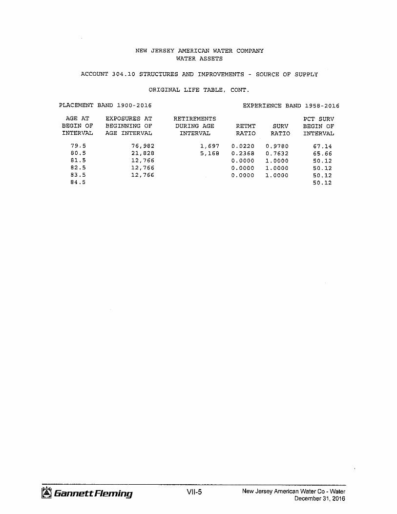


NEW JERSEY AMERICAN WATER COMPANY WATER ASSETS
ACCOUNT 339.10 OTHER PLANT AND EQUIPMENT - INTANGIBLE PLANT
ORIGINAL LIFE TABLE, CONT.
PLACEMENT BAND 1915-2016
AGE AT BEGIN OF INTERVAL
39.5 40.5 41. 5 42.5 43.5 44.5 45.5 46.5 47.5 48.5
49.5 50.5 51.5 52.5 53.5 54.5 55.5 56.5 57.5 58.5
59.5 60.5 61. 5 62.5 63.5 64.5 65.5 66.5 67.5 68.5
69.5 70.5 71.5 72 .5 73.5 74.5 75.5 76.5 77 .5 78.5
EXPOSURES AT BEGINNING OF AGE INTERVAL
21,424
21,424 21,424
179,194
179,194 179,194
~ aannettF/eming
RETIREMENTS DURING AGE
INTERVAL
Vll-143
EXPERIENCE BAND 2014-2016
RETMT RATIO
0.0000
0.0000 0.0000
0.0000
0.0000 0.0000
SURV RATIO
PCT SURV BEGIN OF INTERVAL
New Jersey American Water Co - Water December 31. 2016


[e
w
5 ~ JI ~ s· ll:j <
.- ~ .j>
. (0
ZI
CD " '- CD
ul
CD
'<
)>
3 CD
o~
-CD
2 ~
3-
C" ~
~o
c,,
O
~'
"':E
O
lll
~-
0) ~
(!l z >
>
0:
:::i en
I- z w
(.)
0: w
a.
100 90 ' '
80
70 I
60 I
50 I
40
30
20 ' I
10
0 0
NEW
JE
RS
EY
AM
ER
ICA
N
WA
TER
C
OM
PAN
Y
WA
TER
A
SS
ET
S
AC
CO
UN
T 3
39
.30
O
TH
ER
PL
AN
T
AN
D
EQ
UIP
ME
NT
-
WA
TER
TR
EATM
ENT
SMO
OTH
SU
RV
IVO
R
CU
RV
E
--------~ ~ \
\
\ \ IO
WA
50-
R2.
,
//,.
.
\.,. 1 •
• ,···
·
\ \ \ ~ -
20
40
60
80
AG
E IN
YE
AR
S
100
120


[re g, 5 I'll ::; ;o ~ s· IQ < ' ~ (J
1
~ ZI
"' ,. <.... "' u! "' '< )>
3 "' :,. 0
0 !g
\1l ~
"'
Ql
3 -
c-~
~(")
"'
0 ~
' N
~
0 Q
l
CD~
(!l z > >
a:
::,
Cl)
I- z w
u a: w
a.
100 90
!C
80
70
a!
60
,J
so
,J
40 I
30 I I
20
10
0 0
NEW
JE
RS
EY
AM
ER
ICA
N
WA
TER
C
OM
PAN
Y
WA
TER
A
SS
ET
S
AC
CO
UN
T 3
39
.50
O
TH
ER
PL
AN
T
AN
D
EQ
UIP
ME
NT
-
TR
AN
SM
ISS
ION
A
ND
D
IST
RIB
UT
ION
O
RIG
INA
L A
ND
SM
OO
TH
SUR
VIV
OR
C
UR
VE
S
••••
••
.... ~
l ORIG
INA
L C
UR
VE •
19
94-2
016
EXPE
RIE
NC
E
i-..
1994
-201
4 PL
ACEM
ENTS
~ "' I'\
\ \ IO
WA
35-
R3
\/J4 \
\
\ \ ~ "
-10
20
30
40
50
A
GE
IN
YE
AR
S
60


NEW JERSEY AMERICAN WATER COMPANY WATER ASSETS
ACCOUNT 320.10 STRUCTURES AND IMPROVEMENTS - WATER TREATMENT
CALCULATED REMAINING LIFE DEPRECIATION ACCRUAL RELATED TO ORIGINAL COST AS OF DECEMBER 31, 2016
YEAR (1)
ORIGINAL COST (2)
JUMPING BROOK
CALCULATED ACCRUED
(3)
INTERIM SURVIVOR CURVE .. IOWA 60-SO PROBABLE RETIREMENT YEAR .. 12-2053 NET SALVAGE PERCENT .. 0
2013 2014 2015 2016
211,445.62 26,423.36
113,881.85 277,156.50
3,270,108.20
CANOE BROOK
19,535 1,798 4,826 4,002
375,395
INTERIM SURVIVOR CURVE .. IOWA 60-SO PROBABLE RETIREMENT YEAR .. 12-2072 NET SALVAGE PERCENT .. 0
1961 1963 1965 1966 1968 1970 1973 1990 1991 1992 1996 1997 2011 2012 2013 2014 2015 2016
39.96 5,167.35
698.24 582.24 349.92 882. 71
1,313.65 10,960.93 60,197.95 41,891.86 16,782.84
2,843.70 4,662,356.95
923,994.42 187,732.08
40,564.41 65,101.95
1,291,355.25
7,312,816.41
23 2,871
378 311 182 446 636
3,855 20,634 13,979 4,956
810 481,435
79,741 12,916
2,041 2,018
13,675
640,907
ALLOC. BOOK RESERVE
(4)
27,098 2,494 6,694 5,551
520,721
31 3,875
510 420 246 602 858
5,203 27,849 18,867
6,689 1,093
649,771 107,623 17,432
2,755 2,724
18,457
865,003
FUTURE BOOK ACCRUALS
(5)
REM. LIFE (6)
184,348 32.81 23,929 33.01
107,188 33.22 271,605 33.45
2,749,387
9 25. 77 1,292 26.61
188 27 .44 162 27.84 104 28.64 281 29.43 455 30.58
5,758 36.59 32,349 36.93 23,025 37.26 10,094 38.59 1,750 38.93
4,012,586 43.77 816,372 44.15 170,300 44.53
37,810 44.93 62,378 45.34
1,272,899 45.76
6,447,813
ANNUAL ACCRUAL
(7)
5,619 725
3,227 8,120
84,272
49 7 6 4
10 15
157 876 618 262
45 91,674 18,491
3,824 842
1,376 27,817
146,073
~ Gannett Fleming Vlll-46 New Jersey American Water Co - Water December 31, 2016


NEW JERSEY AMERICAN WATER COMPANY WATER ASSETS
ACCOUNT 334.10 METERS
CALCULATED REMAINING LIFE DEPRECIATION ACCRUAL RELATED TO ORIGINAL COST AS OF DECEMBER 31, 2016
ORIGINAL CALCULATED ALLOC. BOOK FUTURE BOOK REM. YEAR COST ACCRUED RESERVE ACCRUALS LIFE (1) (2) (3) (4) (5) ( 6)
SURVIVOR CURVE .. IOWA 15-Sl NET SALVAGE PERCENT .. 0
1921 448.63 449 449 1930 204.92 205 205 1932 247.76 248 248 1937 523.20 523 523 1959 3,505.39 3,505 3,505 1960 480.94 481 481 1961 2,533.33 2,533 2,533 1962 1,464.07 1,464 1,464 1963 3,416.35 3,416 3,416 1964 2,501.11 2,501 2,501 1965 2,020.42 2,020 2,020 1966 4,805.95 4,806 4,806 1967 4,540.74 4,541 4,541 1968 4,299.07 4,299 4,299 1969 4,112.36 4,112 4,112 1970 5,240.53 5,241 5,241 1971 6,342.93 6,343 6,343 1972 6,924.94 6,925 6,925 1973 7,538.66 7,539 7,539 1974 3,015.09 3,015 3,015 1975 90.59 91 91 1976 1,652.22 1,652 1,652 1977 3,627.68 3,628 3,628 1978 7,520.99 7,521 7,521 1979 13,017.34 13, 017 13,017 1980 15,273.89 15,274 15,274 1981 13,662.26 13,662 13,662 1982 11,986.91 11, 987 11,987 1983 10,923.17 10,923 10,923 1984 31,799.14 31,799 31,799 1985 13,438.98 13,439 13,439 1986 33,990.70 33,991 33,991 1987 238,787.30 236,717 238,787 1988 685,815.71 667,525 685,816 1989 837,713.49 800,293 837,713 1990 1,277,512.02 1,196,607 1,277,512 1991 816,439.71 749,492 816,440 1992 955,672.80 858,834 955,673 1993 2,086,104.67 1,832,998 2,086,105 1994 1,200,413.00 1,029,954 1,200,413 1995 1,548,673.07 1,295,728 1,548,673
ANNUAL ACCRUAL
(7)
~ EiannettF/eming Vlll-81 New Jersey American Water Co - Water December 31, 2016


YEAR ( 1)
NEW JERSEY AMERICAN WATER COMPANY WATER ASSETS
ACCOUNT 340.20 OFFICE FURNITURE AND EQUIPMENT - COMPUTER AND PERIPHERAL EQUIPMENT
CALCULATED REMAINING LIFE DEPRECIATION ACCRUAL RELATED TO ORIGINAL COST AS OF DECEMBER 31, 2016
ORIGINAL COST (2)
CALCULATED ALLOC. BOOK ACCRUED RESERVE
(3) (4)
FUTURE BOOK ACCRUALS
( 5)
REM. LIFE (6)
ANNUAL ACCRUAL
(7)
SURVIVOR CURVE .. 5-SQUARE NET SALVAGE PERCENT .. 0
1993 1996 1998 1999 2001 2004 2005 2006 2007 2008 2009 2010 2011 2012 2013 2014 2015 2016
345,576.14 172,079.99
237.23 3,337.30
12,435.30 1,452.30
16,281.92 79,300.64
348,235.53 264,526.81 153,316.65 951,728.21 207,837.77
1,817,258.78 1,336,388.68 1,866,314.37
727,490.17 3,875,820.22
12,179,618.01
345,576 172,080
237 3,337
12,435 1,452
16,282 79,301
348,236 264,527 153,317 951, 728 207,838
1,635,533 935,472 933,157 218,247 387,582
6,666,337
345,576 172,080
237 3,337
12,435 1,452
16,282 79,301
348,236 264,527 153,317 951,728 207,838
1,817,259 1,336,389 1,866,314
727,490 1,350,732
9,654,530
2,525,088
2,525,088
4.50 561,131
561,131
COMPOSITE REMAINING LIFE AND ANNUAL ACCRUAL RATE, PERCENT .. 4.5 4.61
~ 6annettFleming Vlll-94 New Jersey American Water Co - Water December 31. 2016


