21-761 Finite Difference Methods

Spring 2010

Yekaterina Epshteynnotes by Brendan Sullivan

April 23, 2010

Contents

0 Introduction 2

1 The Finite Difference Method 31.1 Error Analysis . . . . . . . . . . . . . . . . . . . . . . . . . . . . 31.2 Existence and Uniqueness . . . . . . . . . . . . . . . . . . . . . . 71.3 Elliptic Problems in 2-D . . . . . . . . . . . . . . . . . . . . . . . 8

1.3.1 Accuracy and Stability . . . . . . . . . . . . . . . . . . . . 9

2 Iterative Methods for Sparse Linear Systems 102.1 Jacobi and Gauss-Seidel Methods . . . . . . . . . . . . . . . . . . 102.2 Successive Over-Relaxation Method . . . . . . . . . . . . . . . . 12

3 Initial Value Problems for ODEs 123.1 Numerical Solution of ODEs . . . . . . . . . . . . . . . . . . . . . 13

3.1.1 Error Analysis . . . . . . . . . . . . . . . . . . . . . . . . 153.1.2 Crank-Nicholson scheme . . . . . . . . . . . . . . . . . . . 16

4 Initial Value Problems for PDEs 184.1 Heat Equation . . . . . . . . . . . . . . . . . . . . . . . . . . . . 184.2 FDMs for Parabolic Problems . . . . . . . . . . . . . . . . . . . . 19

4.2.1 Error Analysis . . . . . . . . . . . . . . . . . . . . . . . . 204.3 Mixed IVP . . . . . . . . . . . . . . . . . . . . . . . . . . . . . . 21

4.3.1 Implicit Scheme . . . . . . . . . . . . . . . . . . . . . . . 234.3.2 Crank-Nicholson Scheme . . . . . . . . . . . . . . . . . . . 24

4.4 FDMs for Hyperbolic Equations . . . . . . . . . . . . . . . . . . . 254.4.1 First Order Scalar Equation . . . . . . . . . . . . . . . . . 254.4.2 Characteristic tracing and interpolation . . . . . . . . . . 27

4.5 The CFL Condition . . . . . . . . . . . . . . . . . . . . . . . . . 284.6 Modified Equations . . . . . . . . . . . . . . . . . . . . . . . . . . 29

4.6.1 Higher Order Methods . . . . . . . . . . . . . . . . . . . . 30

1

4.6.2 Mixed Equations and Fractional Step Methods . . . . . . 314.7 More Mixed Problems . . . . . . . . . . . . . . . . . . . . . . . . 334.8 Implicit-Explicit Methods . . . . . . . . . . . . . . . . . . . . . . 35

5 Analyses of Finite Difference Schemes 365.1 Fourier Analysis . . . . . . . . . . . . . . . . . . . . . . . . . . . 365.2 Von Neumann Analysis . . . . . . . . . . . . . . . . . . . . . . . 38

5.2.1 Stability Condition . . . . . . . . . . . . . . . . . . . . . . 405.3 Stability conditions for variable coefficients . . . . . . . . . . . . 43

5.3.1 Stability of Lax-Wendroff and Crank-Nicholson . . . . . . 44

6 Solution of Linear Systems 456.1 Method of steepest descent . . . . . . . . . . . . . . . . . . . . . 456.2 Conjugate Gradient Method . . . . . . . . . . . . . . . . . . . . . 47

0 Introduction

Our main interest is in solving initial boundary value problems.

Example 0.1. Consider the Poisson equation, a standard example of an ellipticPDE

−∆u = f in Ωu = g(x) on Γ

where x = (x1, x2, . . . , xn) and Γ ⊆ ∂Ω. Recall that ∆u =∑j∂2u∂x2

j. The second

line above is the boundary data, and such a condition is known as Dirichletboundary data. We will also consider Neumann boundary data

∂u

∂n= g(x) on Γ

where n is the outward unit normal, and so ∂u∂n = ∇u · n. We will also consider

Robin boundary data∂u

∂n+ βu(x) = g(x) on Γ

More generally, an elliptic PDE is of the form Au = f for some operator

Au := −d∑

i,j=1

∂

∂xi

(aij(x)

∂u

∂xj

)+

d∑j=1

bj(x)∂u

∂xj

with A(x) := (aij(x))di,j=1 a positive-definite matrix.

Example 0.2. Consider the heat equation

∂u∂t −∆u = f(x, t)u(x, 0) = u0(x)

plus some boundary data. This is an example of a parabolic (linear) PDE.

2

Example 0.3. Consider the wave equation

∂2u

∂t2−∆u = f(x, t)

This is an example of a hyperbolic PDE.

1 The Finite Difference Method

Consider a simple FDM on the ODE

u′′(x) = f(x) in [0, 1]u(0) = αu(1) = β

(1)

Divide [0, 1] into subintervals by identifying the nodes xj = jh with h = 1m+1 ,

for j = 0, 1, . . . ,m+ 1. We seek to approximate uj := u(xj). We replace u′′ byusing the centered difference approximation

u′′(xj) ≈uj−1 − 2uj + uj+1

h2= f(xj) , j = 1, 2, . . . ,m

and u0 = u(0) = α and um+1 = u(1) = β. Then we define the solution vectorU = [u1, u2, . . . , um]T and we seek the solution to the linear system AU = Fwhere

A =1h2

−2 1 01 −2 1 00 1 −2 1 0

. . .0 1 −2 1

0 1 −2

and

F =

f(x1)− α

h2

f(x2)...

f(xm)− βh2

1.1 Error Analysis

The global error of the approximation U we obtain is give by E = U −u, whereu is the true solution vector. To quantify this error, we use various norms:

1. ‖E‖∞ = max1≤j≤m |Ej | = max1≤j≤m |Uj − uj |

2. ‖E‖1 = h∑mj=1 |Ej |

3. ‖E‖2 =(h∑mj=1 |Ej |2

)1/2

3

The space Rd is finite-dimensional, so all of these norms are equivalent, topo-logically, but the constant of equivalence typically involves some power of h, soconvergence rates may vary in different norms.

Definition 1.1. We consider the local truncation error τ = [τj ]mj=1 given by

τj :=u(xj−1)− 2u(xj) + u(xj+1)

h2− f(xj) , 1 ≤ j ≤ m

By Taylor’s Theorem, we can write

u(xj−1) = u(xj)− hu′(xj) +h2

2u′′(xj)−

h3

6u′′′(xj) +

h4

24u(4)(xj)

− h5

120u(5)(xj) +O(h6)

and

u(xj+1) = u(xj) + hu′(xj) +h2

2u′′(xj) +

h3

6u′′′(xj) +

h4

24u(4)(xj)

+h5

120u(5)(xj) +O(h6)

so then

τj =h2

12u(4)(xj) + u′′(xj) +O(h4)− f(xj) =

h2

12u(4)(xj) +O(h4)

and so τj = O(h2) as h→ 0.Thinking of τ = Au − F and AU = F , then we can subtract and write

the global error as AE = −τ . Since each depends on h, we typically writeAhEh = −τh. Assuming that (Ah)−1 exists, we can write the error as

Eh = −(Ah)−1

τh

and so‖Eh‖ =

∥∥∥(Ah)−1∥∥∥ · ‖τh‖

in any norm. In order to have ‖Eh‖ = O(‖τh‖), we need∥∥∥(Ah)−1

∥∥∥ ≤ C for all

sufficiently small h. If this holds, then ‖Eh‖ ≤ C‖τh‖.

Definition 1.2. Suppose a FDM for a linear BVP gives a sequence of matrixequations AhUh = Fh, where h is the width of the mesh. We say that themethod is stable provided

(Ah)−1 exists ∀h < h0 and if ∃C independent of h

such that∥∥∥(Ah)−1

∥∥∥ ≤ C ∀h < h0.

Remark 1.3. Note that stability in one norm⇒ stability in any equivalent norm.

4

Definition 1.4. We say a method is consistent with the original ODE and BCsif ‖τh‖ → 0 as h→ 0.

Definition 1.5. We say a method is convergent if ‖Eh‖ → 0 as h→ 0.

Theorem 1.6 (Fundamental Theorem of FDs). If a scheme is consistent andstable, then it is convergent.

Proof. By assumption, we may write

‖Eh‖ ≤∥∥∥(Ah)−1

∥∥∥ · ‖τh‖ ≤ C‖τh‖ → 0

as h→), which shows convergence.

In general, we can say that stability and order O(hp) of local truncationerror implies order O(hp) of global error. Note that the order does depend onthe choice of norm.

Note that in general there is a practical tradeoff between complexity of pro-gramming and scheme convergence rate. Also, it is vastly more inefficient (inMatlab) to use the command U =inv(A) ·F to solve the linear system, since thisuses at least n2 operations, whereas U = A \ F (or some command like that)is more efficient, since it produces the product without actually computing theinverse.

It is a good idea to check for stability at the continuum level, to see whetherwe have a chance of achieving stability for the discretized scheme. For this spe-cific model problem, we can use the Poincare and Cauchy-Schwarz inequalitiesto take ∆E = τ , multiply both sides by E, then integrate by parts and write

c

∫E2 ≤

∫|∇E|2 = −

∫τE ≤

(∫τ2

)1/2(∫E2

)1/2

and then divide, yielding ‖E‖2 ≤ c‖τ‖2. For the discretized scheme, we wantto write

‖Eh‖2 =∥∥(Ah)−1τh

∥∥2≤∥∥(Ah)−1

∥∥∥∥τh∥∥2

and the appropriate choice for the norm on (Ah)−1 is the operator norm:

‖A‖2 = supv 6=~0

‖Av‖22‖v‖22

Since A is symmetric, for this specific problem, we know ∃ eigenvalues λ1, . . . , λmand eigenvectors v1, . . . , vm such that v =

∑i αivi, and Av =

∑i αiλivi. Then,

‖A‖2 = supv 6=~0

∑α2iλ

2i∑

i α2i

= maxiλ2i

and so ‖A‖ = maxi |λi|. We now introduce the eigenfunctions ui = sin(iπx)and upj = sin(πpjh) for h = 1

m+1 and j, p = 1, . . . ,m. Then

λp =2h2

(cos(πph)− 1) ≈ −π2 +O(h2)

5

since cosx ≥ 1− x2

2 . Then the eigenvalues of (Ah)−1 are∣∣∣∣ 1λp

∣∣∣∣ ∼ ∣∣∣∣ −1p2π2

∣∣∣∣ & 1π2

and so‖Eh‖2 ≤

1π2‖τh‖

Now, what about Neumann boundary conditions? We investigate the prob-lem

u′′ = f , u′(0) = b , u(1) = β

We have three different ideas to try.

1. Try setting u0 = α and u1−u0h = b. Then we know

u(x1)− u(x0) = u′(x0)h+u′′(xc)

2h2

where u is the actual solution and xc is some point guaranteed by theMean Value Theorem. Then we have

u(x1)− u(x0

h− b =

f(xc)2

h

which yields an error of order h, which is not as good as before.

2. To motivate the next idea, recall that

limh→0

∣∣∣∣f(x+ h)− f(x)h

− f ′(x)∣∣∣∣ = 0

but

limh→0

∣∣∣∣ 1h(f(x+ h)− f(x− h)

2h− f ′(x)

)∣∣∣∣ = 0

As such, we “introduce” u−1 and set

u−1 − 2u0 + u1

h2= f(x0) and

u1 − u−1

2h= b

Really, we use the second equation to “find” u−1 and plug this value intothe first equation.

3. The “best” idea yields a second-order accurate approximation. We set

1h

(−3

2u0 + 2u1 −

u2

2

)= b

Example 1.7. The problem

u′′ ≡ 0 , u′(0) = 1 , u′(1) = 0

has no solution. Specifically, the matrix in the discrete scheme becomes singular.This illustrates how things can go wrong.

6

Recall the 3rd approach above. This is an illustration of the more generalmethod of undetermined coefficients. Suppose that

u′(0) = au(0) + bu(h) + cu(2h)

Applying Taylor’s Theorem, we have

u(h) = u(0) + hu′(0) +h2

2u′′(0) +

h3

6u′′′(ξ1) for someξ1 ∈ (0, h) (2)

and

u(2h) = u(0) + 2hu′(0) + 2h2u′′(0) +4h3

3u′′′(ξ2) for some ξ2 ∈ (0, 2h) (3)

Combining these, we have

u′(0) ≈ au(0) + b

(u(0) + hu′(0) +

h2

2u′′(0) +

h3

6u′′′(ξ1)

)+ c

(u(0) + 2hu′(0) + 2h2u′′(0) +

4h3

3u′′′(ξ2)

)= (a+ b+ c)u(0) + (b+ 2c)hu′(0) +

(b+ 4c

2

)h2u′′(0) +O(h3)

so we require

a+ b+ c = 0 , b+ 2c =1h

,b+ 4c

2= 0

to make u′(0) ≈ u′(0) +O(h3). The solution is

a = − 32h

, b =2h

, c = − 12h

This is precisely approach 3 from before. Note that b + c ∼ 1h which yields an

O(h2) error overall.

1.2 Existence and Uniqueness

Example 1.8. Consider solving

u′′(x) = f(x) , u′(0) = σ0 , u′(1) = σ1

This problem is not well-posed. A solution will be of the form

u(x) =x2

2+ c1x+ c2

which can be obtained by integrating, with c1 = σ0 = σ1 − 1. Therefore, weeither have infinitely-many solutions or none. The discretized version of this

7

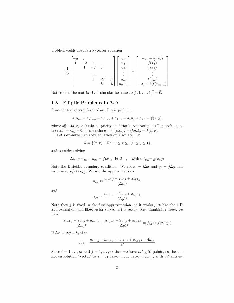
problem yields the matrix/vector equation

1h2

−h h1 −2 1

1 −2 1. . .1 −2 1

h −h

u0

u1

u2

...umum+1

=

−σ0 + h2 f(0)

f(x1)f(x2)

...f(xm)

−σ1 + h2 f(xm+1)

Notice that the matrix Ah is singular because Ah[1, 1, . . . , 1]T = ~0.

1.3 Elliptic Problems in 2-D

Consider the general form of an elliptic problem

a1uxx + a2uxy + a3uyy + a4ux + a5uy + a6u = f(x, y)

where a22 − 4a1a3 < 0 (the ellipticity condition). An example is Laplace’s equa-

tion uxx + uyy = 0, or something like (kux)x + (kuy)y = f(x, y).Let’s examine Laplace’s equation on a square. Set

Ω = (x, y) ∈ R2 : 0 ≤ x ≤ 1, 0 ≤ y ≤ 1

and consider solving

∆u := uxx + uyy = f(x, y) in Ω , with u ∂Ω= g(x, y)

Note the Dirichlet boundary condition. We set xi = i∆x and yj = j∆y andwrite u(xi, yj) ≈ ui,j . We use the approximations

uxx ≈ui−1,j − 2ui,j + ui+1,j

(∆x)2

anduyy ≈

ui,j−1 − 2ui,j + ui,j+1

(∆y)2

Note that j is fixed in the first approximation, so it works just like the 1-Dapproximation, and likewise for i fixed in the second one. Combining these, wehave

ui−1,j − 2ui,j + ui+1,j

(∆x)2+ui,j−1 − 2ui,j + ui,j+1

(∆y)2= fi,j ≈ f(xi, yj)

If ∆x = ∆y = h, then

fi,j =ui−1,j + ui+1,j + ui,j−1 + ui,j+1 − 4ui,j

h2

Since i = 1, . . . ,m and j = 1, . . . ,m then we have m2 grid points, so the un-known solution “vector” is u = u11, u12, . . . , u21, u22, . . . , umm with m2 entries.

8

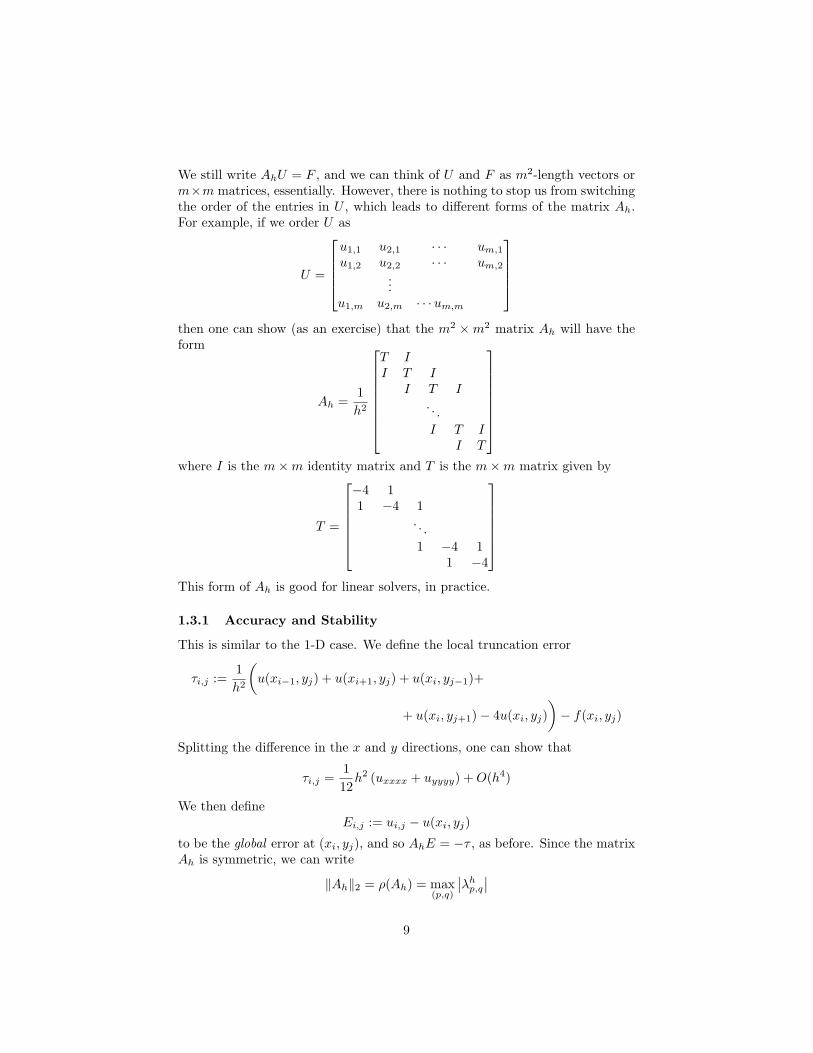
We still write AhU = F , and we can think of U and F as m2-length vectors orm×m matrices, essentially. However, there is nothing to stop us from switchingthe order of the entries in U , which leads to different forms of the matrix Ah.For example, if we order U as

U =

u1,1 u2,1 · · · um,1u1,2 u2,2 · · · um,2

...u1,m u2,m · · ·um,m

then one can show (as an exercise) that the m2 ×m2 matrix Ah will have theform

Ah =1h2

T II T I

I T I. . .I T I

I T

where I is the m×m identity matrix and T is the m×m matrix given by

T =

−4 11 −4 1

. . .1 −4 1

1 −4

This form of Ah is good for linear solvers, in practice.

1.3.1 Accuracy and Stability

This is similar to the 1-D case. We define the local truncation error

τi,j :=1h2

(u(xi−1, yj) + u(xi+1, yj) + u(xi, yj−1)+

+ u(xi, yj+1)− 4u(xi, yj))− f(xi, yj)

Splitting the difference in the x and y directions, one can show that

τi,j =112h2 (uxxxx + uyyyy) +O(h4)

We then defineEi,j := ui,j − u(xi, yj)

to be the global error at (xi, yj), and so AhE = −τ , as before. Since the matrixAh is symmetric, we can write

‖Ah‖2 = ρ(Ah) = max(p,q)

∣∣λhp,q∣∣9

where ρ indicates the spectral radius, so λhp,q are eigenvalues of Ah. It can beshown that ∥∥A−1

h

∥∥2

=(

min1≤p,q≤m

∣∣λhp,q∣∣)−1

≈ 12π2

for sufficiently small h, which implies∥∥A−1

h

∥∥ ≤ C ∀h < h0 small enough. Wecan then write

AhE = −τ ⇒ ‖E‖ ≤∥∥A−1

h

∥∥2‖τ‖2 ≤ C ‖τ‖2

so the method is stable with respect to ‖ · ‖2, and ‖E‖2 = O(h2).

2 Iterative Methods for Sparse Linear Systems

We will examine the Jacobi, Gauss-Seidel, and Successive Over-relaxation meth-ods.

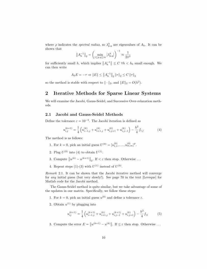
2.1 Jacobi and Gauss-Seidel Methods

Define the tolerance ε = 10−5. The Jacobi iteration is defined as

u(k=1)i,j =

14

(u

(k)i−1,j + u

(k)i+1,j + u

(k)i,j+1 + u

(k)i,j−1

)− h2

4fi,j (4)

The method is as follows:

1. For k = 0, pick an initial guess U (0) = [u(0)1,1, . . . , u

(0)m,m]T .

2. Plug U (0) into (4) to obtain U (1).

3. Compute∥∥u(k) − u(k+1)

∥∥2. If < ε then stop. Otherwise . . .

4. Repeat steps (1)-(3) with U (1) instead of U (0).

Remark 2.1. It can be shown that the Jacobi iterative method will convergefor any initial guess (but very slowly!). See page 70 in the text [Leveque] forMatlab code for the Jacobi method.

The Gauss-Seidel method is quite similar, but we take advantage of some ofthe updates in our matrix. Specifically, we follow these steps:

1. For k = 0, pick an initial guess u(0) and define a tolerance ε.

2. Obtain u(1) by plugging into

u(k+1)ij =

14

(u

(k+1)i−1,j + u

(k)i+1,j + u

(k+1)i,j−1 + u

(k)i,j+1

)− h2

4fij (5)

3. Compute the error E =∥∥u(k+1) − u(k)

∥∥. If ≤ ε then stop. Otherwise . . .

10

4. Repeat steps (1)-(3) with u(1) instead of u(0).

Example 2.2. Consider the usual ODE u′′(x) = f(x), u(0) = α, u(1) = β. Whenwe solve using the Finite Difference Method, we obtain a tridiagonal system,due to the relation

1h2

(ui+1 − 2ui + ui−1) = fi

Applying Jacobi, we have

u(k+1)i =

12

(u

(k)i−1 + u

(k)i+1 − h

2fi

)and applying Gauss-Seidel, we have

u(k+1)i =

12

(u

(k+1)i−1 + u

(k)i+1 − h

2fi

)This yields a system Au = f . The goal of this method will be to write A =M −N for some choice of matrices M,N , so that Mu = Nu+ f , which we willwrite as

Mu(k+1) = Nu(k) + f

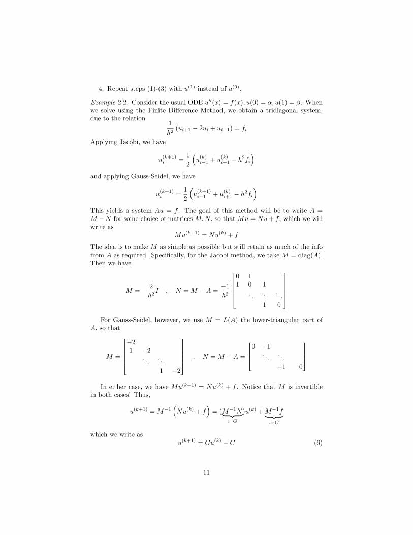
The idea is to make M as simple as possible but still retain as much of the infofrom A as required. Specifically, for the Jacobi method, we take M = diag(A).Then we have

M = − 2h2I , N = M −A =

−1h2

0 11 0 1

. . . . . . . . .1 0

For Gauss-Seidel, however, we use M = L(A) the lower-triangular part of

A, so that

M =

−21 −2

. . . . . .1 −2

, N = M −A =

0 −1. . . . . .

−1 0

In either case, we have Mu(k+1) = Nu(k) + f . Notice that M is invertible

in both cases! Thus,

u(k+1) = M−1(Nu(k) + f

)= (M−1N︸ ︷︷ ︸

:=G

)u(k) +M−1f︸ ︷︷ ︸:=C

which we write asu(k+1) = Gu(k) + C (6)

11

Suppose uT is the true solution of the original system, so AuT = f . Then wetake Equation (6) and take a limit as k → ∞: uT = GuT + C; i.e. uT is thefixed point for Equation (6).

Will this method converge for all u0? To answer this question, we define theerror

e(k+1) := u(k+1) − uT ≡ Ge(k)

Iterating, we have e(k) = Gke(0), so for convergence we need Gk → 0 in somesense. We know that Gk → 0 if σ(G) < 1 (the spectral radius σ); if this holds,the we obtain convergence for any initial guess u0! Note:

σ (GJacobi) = |cos(πh)| < 1

for h < 1, andσ (GGauss-Seidel) ≈ 1− π2h2 +O(h4)

if h is small enough (i.e. ∀0 < h < h0). Note that as h → 0, σ(G) → 1, soconvergence rate gets slower, but the convergence is still guaranteed for anyguess u0.

2.2 Successive Over-Relaxation Method

RecalluGSi =

12

(u

(k+1)i−1 + u

(k)i+1 − h

2fi

)is the k + 1-th iterate for the Gauss-Seidel method. We use this to define

u(k+1)i = u

(k)i + ω

(uGSi − u

(k)i

), 0 < ω < 2

which can be written as

u(k+1)i =

ω

2

(u

(k+1)i−1 + u

(k)i+1 − h

2fi

)+ (1− ω)u(k)

i

Notice that ω = 1 corresponds to the Gauss-Seidel method.

3 Initial Value Problems for ODEs

The goal of this section is to prepare for the study of elliptic and parabolicPDEs. We consider the ODE

u′ + au = f(t) , t > 0u(0) = γ

(7)

To solve this, we introduce the integrating factor eat and multiply both sides ofEquation (7) by eat to get

u′eat + aeatu = f(t)eat

12

Then, we recognize the LHS as a derivative to write

d

dt

(eatu

)= eatf(t)

and then integrate both sides with respect to t to get

eatu = eatu t=0 +∫ t

0

eatf(s) ds = γ +∫ t

0

eatf(s) ds

This gives us the solution

u(t) = e−atγ +∫ t

0

exp(−a(t− s))f(s) ds (8)

If a > 0, then we have the estimate

|u(t)| ≤ |γ|+∫ t

0

|f(s)| ds , t ≥ 0

If we can obtain an estimate like this, then we say that u′+au = f(t) is a stableODE (i.e. the solution is bounded by initial data and the RHS). Why is thisthe definition of stability? To see why, consider the two problems

u′1 + au1 = f1(t) , t > 0u1(0) = γ1

andu′2 + au2 = f2(t) , t > 0

u2(0) = γ2

and assume both are stable. Then we can consider the (difference) problem

(u1 − u2)′ + a(u1 − u2) = f1(t)− f2(t) , t > 0(u1 − u2)(0) = γ1 − γ2

and we know that we have the stability estimate

|u1(t)− u2(t)| ≤ |γ1 − γ2|+∫ t

0

|f1(s)− f2(s)| ds

This implies that small perturbations to initial data and/or the RHS do notproduce large changes in the solution. Specifically, consider f2 = f1 + ε1 andγ2 = γ1 + ε2 for some small ε1, ε2.

3.1 Numerical Solution of ODEs

Consider the ODE in Equation (7), and apply the Forward Euler method, givenby

U ′(tn) ≈ Un − Un−1

∆t

13

where Un ≈ u(tn), tn = n∆t, ∆ = tN . The Forward Euler (FE) approximation

of the ODE becomes

Un−Un−1

∆t + aUn−1 = f(tn, U

n−1)

, n ≥ 1U0 = γ

(9)

To solve this, we apply the following steps:

1. For, n = 1 we useU1 − U0

∆t+ aU0 = f

(t, U0

)to find U1:

U1 = ∆t · f(t, U0

)+ (1− a∆t)U0

We write U1 ≈ u(t1) = u(∆t).

2. Next, set U0 = U1.

3. Repeat steps 1 and 2 to obtain U2. Continue until UN .

This method is an explicit time-stepping algorithm, and be coded via a loopover time steps ∆t = T

N to solve the ODE on [0, T ] with N subintervals.Let’s consider a specific model problem where f (T,U) ≡ 0, and investigate

the accuracy and stability of the method.

Un−Un−1

∆t + aUn−1 = 0 , n ≥ 1U0 = γ

(10)

We have

Un = (1− a∆t)Un−1 , Un−1 = (1− a∆t)Un−2 , · · · ,U2 = (1− a∆t)U1 , U1 = (1− a∆t)U0

and this allows us to write a recursive formula

u(tn) ≈ Un = (1− a∆t)n · γ

For t = tn fixed, we have

limn→∞

Un = limn→∞

(1− a t

n

)n= γ exp(−at)

so that ∆t → 0 ⇒ Un → u(tn). Q: How fast is this convergence? That is,what is the error |Un − u(tn)| and how does it change with n?

Assume a > 0, and let’s take ∆t such that 1 ≥ 1− a∆t ≥ −1; i.e. ∆t ≤ 2a .

ThenUn = (1− a∆t)n · γ ⇒ |Un| ≤ |γ|

However, if ∆t > 2a , then Un will grow with n; i.e. |Un| → ∞ as n→∞. That

is, the scheme will not be stable.

14

3.1.1 Error Analysis

Observe that we can write the error as

Un − u(tn) = (1− a∆t)n γ − exp(−atn)γ = (1− a∆t)n γ − exp(−an∆t)γ= (1− a∆t)n γ − (exp(−a∆t))n γ= γ ((1− a∆t)n − (exp(−a∆t))n)

= γ (1− a∆t− exp(−a∆t)) ·((1− a∆t)n−1

+(1− a∆t)n−2 exp(−a∆t) + · · ·+ (exp(−a∆t))n−1)

= (1− a∆t− exp(−a∆t))n−1∑k=0

(1− a∆t)j exp(−(n− 1− j)a∆t)

where we have applied the identity

an − bn = (a− b) ·(an−1 + abn−2 + a2bn−3 + · · ·+ an−2b+ bn−1

)Thus,

|Un − u(tn)| ≤ |1− a∆t− exp(−a∆t)| ·

·

∣∣∣∣∣∣n−1∑j=0

(1− a∆t)j exp(−(n− 1− j)a∆t)

∣∣∣∣∣∣ · |γ|≤ a2(∆t)2

2

n−1∑j=0

|γ| = a2(∆t)2

2· n|γ|

=a2∆t

2tn|γ| = O(∆t)

since|1− a∆t− exp(−a∆t)| ≤ 1

2a2(∆t)2

and each term in the sum above satisfies∣∣(1− a∆t)j∣∣ · |exp(−(n− 1− j)a∆t)| ≤ 1

Thus, a∆t ≤ 2 is the so-called stability restriction.****** insert picture *****Now, let’s examine the same ODE in Equation (7) using the Backward Euler

(BE) method (an implicit time scheme). That is, we write

Un−Un−1

∆t + aUn = f (tn, Un) , n ≥ 1U0 = γ

(11)

We solve this by performing the following steps:

1. Input U0, ∆t = tn .

15

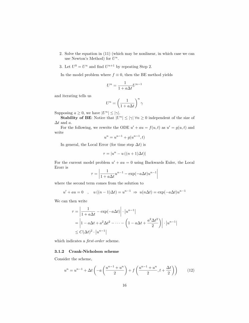
2. Solve the equation in (11) (which may be nonlinear, in which case we canuse Newton’s Method) for Un.

3. Let U0 = Un and find Un+1 by repeating Step 2.

In the model problem where f ≡ 0, then the BE method yields

Un =1

1 + a∆tUn−1

and iterating tells us

Un =(

11 + a∆t

)nγ

Supposing a ≥ 0, we have |Un| ≤ |γ|.Stability of BE: Notice that |Un| ≤ |γ| ∀n ≥ 0 independent of the size of

∆t and a.For the following, we rewrite the ODE u′ + au = f(u, t) as u′ = g(u, t) and

writeun = un−1 + g(un−1, t)

In general, the Local Error (for time step ∆t) is

τ = |un − u ((n+ 1)∆t)|

For the current model problem u′ + au = 0 using Backwards Euler, the LocalErorr is

τ =∣∣∣∣ 11 + a∆t

un−1 − exp(−a∆t)un−1

∣∣∣∣where the second term comes from the solution to

u′ + au = 0 , u ((n− 1)∆t) = un−1 ⇒ u(n∆t) = exp(−a∆t)un−1

We can then write

τ =∣∣∣∣ 11 + a∆t

− exp(−a∆t)∣∣∣∣ · ∣∣un−1

∣∣=∣∣∣∣1− a∆t+ a2∆t2 − · · · −

(1− a∆t+

a2∆t2

2

)∣∣∣∣ · ∣∣un−1∣∣

≤ C(∆t)2 ·∣∣un−1

∣∣which indicates a first-order scheme.

3.1.2 Crank-Nicholson scheme

Consider the scheme,

un = un−1 + ∆t(−a(un−1 + un

2

)+ f

(un−1 + un

2, t+

∆t2

))(12)

16

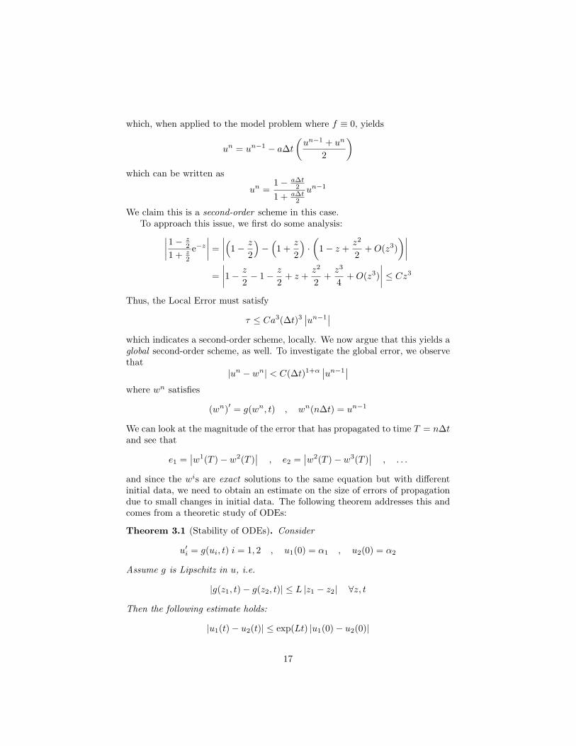
which, when applied to the model problem where f ≡ 0, yields

un = un−1 − a∆t(un−1 + un

2

)which can be written as

un =1− a∆t

2

1 + a∆t2

un−1

We claim this is a second-order scheme in this case.To approach this issue, we first do some analysis:∣∣∣∣1− z

2

1 + z2

e−z∣∣∣∣ =

∣∣∣∣(1− z

2

)−(

1 +z

2

)·(

1− z +z2

2+O(z3)

)∣∣∣∣=∣∣∣∣1− z

2− 1− z

2+ z +

z2

2+z3

4+O(z3)

∣∣∣∣ ≤ Cz3

Thus, the Local Error must satisfy

τ ≤ Ca3(∆t)3∣∣un−1

∣∣which indicates a second-order scheme, locally. We now argue that this yields aglobal second-order scheme, as well. To investigate the global error, we observethat

|un − wn| < C(∆t)1+α∣∣un−1

∣∣where wn satisfies

(wn)′ = g(wn, t) , wn(n∆t) = un−1

We can look at the magnitude of the error that has propagated to time T = n∆tand see that

e1 =∣∣w1(T )− w2(T )

∣∣ , e2 =∣∣w2(T )− w3(T )

∣∣ , . . .

and since the wis are exact solutions to the same equation but with differentinitial data, we need to obtain an estimate on the size of errors of propagationdue to small changes in initial data. The following theorem addresses this andcomes from a theoretic study of ODEs:

Theorem 3.1 (Stability of ODEs). Consider

u′i = g(ui, t) i = 1, 2 , u1(0) = α1 , u2(0) = α2

Assume g is Lipschitz in u, i.e.

|g(z1, t)− g(z2, t)| ≤ L |z1 − z2| ∀z, t

Then the following estimate holds:

|u1(t)− u2(t)| ≤ exp(Lt) |u1(0)− u2(0)|

17

This is useful in our current analysis since we can write

|un(T )− u(T )| ≤ |un(T )− wn(T )|+∣∣wn(T )− wn−1(T )

∣∣++ · · ·+

∣∣w2(T )− w1(T )∣∣

≤ (∆t)1+α + c exp (L(2∆t)) (∆t)1+α∣∣un−1

∣∣++ · · ·+ c exp (L(n∆t)) (∆t)1+αu0

≤ (∆t)1+αc exp (LT )T

∆tM

∼ (∆t)α

4 Initial Value Problems for PDEs

4.1 Heat Equation

Consider the initial value problem

ut −∆u = 0 in Rd × R+

u(·, 0) = v in Rd(13)

The solution to (13) is given by

u(x, t) = (4πt)−d2

∫Rd

v(y) exp(−|x− y|

2

4t

)dy (14)

and the so-called fundamental solution is given by

u(x, t) = (4πt)−d2 exp

(−|x|

2

4t

)(15)

Theorem 4.1. If v is a bounded continuous function on Rd then the functionu(x, t) defined by Equation (15) is a solution of the Heat equation (13) for allt > 0 and u→ v as t→ 0.

In a general setting, we consider a system like

ut −∆u = f in Ω× I := Ω× (0, T )u = g on Γ× I := ∂Ω× I

u(·, 0) = v in Ω(16)

We also define the parabolic boundary

Γp =(Γ× I

)∪ (Ω× t = 0)

which is the boundary of the parabolic cylinder, minus the lid, so to speak.

Theorem 4.2. Let u be a smooth function and assume that ut − ∆u ≤ 0 inΩ× I. Then u attains its maximum on the parabolic boundary.

18

Theorem 4.3. The solution of (16) satisfies

sup(x,t)∈Ω×I

|u(x, t)| ≤ max

maxx∈Γ×I

|g|,maxx∈Ω|v|

+r2

2dmax

(x,t)∈Ω×I|f |

where r is the radius of the smallest ball that contains Ω.

Theorem 4.4. The initial value problem (13) has at most one solution that isbounded in Rd × [0, T ], where T is arbitrary.

4.2 FDMs for Parabolic Problems

Consider the PDE

ut = uxx in R× R+

u(·, 0) = v in R(17)

for some given function v. Assuming that v is smooth and bounded, we have thefollowing properties:

1. The problem (17) has a unique solution.

2. supx|u(x, t)| ≤ sup

x|v(x)| for every t ≥ 0.

3. The solution is given by

u(x, t) =1√4πt

∫ ∞−∞

exp(−|x− y|

2

4t

)v(y) dy

which is just a special case of Equation (14) with d = 1.

4. |u(·, t)|C4 ≤ |v|C4 , where |v|C4 := max|α|≤4

|Dαv|.

To apply the Finite Difference Method, we need to discretize in time andspace. We introduce a grid of mesh points: (x, t) = (xj , tn) where xj = jh withj ∈ Z and tn = n∆t with n ∈ N.

The simplest FD scheme is given by

ut(xj , tn) ≈un+1j − unj

∆t=unj+1 − 2unj + unj−1

h2≈ uxx(xj , tn)

where un+1j ≈ u(xj , tn+1) and unj ≈ u(xj , tn) for j ∈ Z and n ∈ N. This is an

(explicit) Forward Euler method, so we can write this as the system

un+1j = (E∆tu

n)j := λunj−1 + (1− 2λ)unj + λunj+1 for n ∈ N, j ∈ Z

u0j = vj

(18)

where λ := ∆th2 . This is a recursive formula, so we can write

unj =(E∆tu

n−1)j

=(E∆tE∆tu

n−2)j

= · · · = (En∆tu0)j

19

Assume that 0 ≤ λ ≤ 12 so that all of the coefficients above in the operator E∆t

are ≥ 0. This allows us to write

|un+1j | =

∣∣∣(E∆tun)j∣∣∣ ≤ λ|unj−1|+ (1− 2λ)|unj |+ λ|unj+1|

≤ λ supj∈Z|unj |+ (1− 2λ) sup

j∈Z|unj |+ λ sup

j∈Z|unj |

= supj∈Z|unj |

Iterating this procedure yields the bound supj |u0j | = supj |vj |, and so

supj∈Z|unj | ≤ sup

j∈Z|vj |

This is the stability estimate for the FD scheme.

Example 4.5. Let’s consider what happens for an unstable scheme. Supposeλ > 1

2 and ∆t > h2

2 . Let vj = (−1)jε for ε > 0 small. Then supj |vj | = ε.Notice that

u1j =

(λ(−1)j−1 + (1− 2λ)(−1)j + λ(−1)j+1

)ε = (1− 4λ)(−1)jε

Iterating, we obtain

unj = (1− 4λ)n(−1)jε ⇒ supj∈Z|unj | = (4λ− 1)nε −−−−→

n→∞∞

4.2.1 Error Analysis

Consider λ ≤ 12 . We want to characterize maxj

∣∣unj − unj ∣∣, where unj = u(xj , tn)the true solution. We write xj ∈ (xj−1, xj+1) and tn ∈ (tn, tn+1). Also, noticethat utt = (ut)xx = uxxxx. We start to define the local truncation error by usingu in Equation (4.2)

τnj : =un+1j − unj

∆t−unj+1 − 2unj + unj−1

h2− (ut − uxx)︸ ︷︷ ︸

=0

=

(un+1j − unj

∆t− ut(xj , tn)

)−(unj+1 − 2unj + unj−1

h2− uxx(xj , tn)

)and then using the Taylor expansion around tn

un+1j = u(xj , tn+1) = u(xj , tn) + ut(xj , tn)∆t+

∆t2

2utt(xj , tn)

= unj + ∆tut(xj , tn) +∆t2

2utt(xj , tn)

This allows us to rewrite the first term in the difference above as

un+1j − unj

∆t− ut(xj , tn) =

∆t2utt(xj , tn)

20

Likewise, we can use the Taylor expansion around xj to write

unj+1 = u(xj+1, tn) = unj + hux(xj , tn) +h2

2uxx(xj , tn)

+h3

3!uxxx(xj , tn) +

h4

4!uxxxx(xj , tn)

and

unj−1 = u(xj−1, tn) = unj + hux(xj , tn) +h2

2uxx(xj , tn)

+h3

3!uxxx(xj , tn) +

h4

4!uxxxx(xj−1, tn)

Combining these in the second term in the difference equation above yields

unj+1 − 2unj + unj−1

h2− uxx(xj , tn) =

h2

24(uxxxx(xj , tn) + uxxxx(xj−1, tn))

Finally, this gives us the local truncation error

τnj =12

∆tutt(xj , tn)− h2

24(uxxxx(xj , tn) + uxxxx(xj−1, tn)) (19)

Then,

maxj

∣∣τnj ∣∣ ≤ ∆t2

maxj,n|utt|+

h2

12|u(·, tn)|C4

where|u(·, tn)|C4 = max

|α|≤4|Dα

xu(·, tn)|

Recall that |u(·, tn)|C4 ≤ |v|C4 and utt = uxxxx, so then

maxj|τnj | ≤

h2

3|v|C4

Theorem 4.6. Let un ≈ u(xj , tn) for j ∈ Z for u a solution to the heat equation.Let λ = ∆t

h2 ≤ 12 . Then ∃C such that

maxj∈Z|un − un| ≤ Ctnh2|v|C4

where C is independent of ∆ and h.

4.3 Mixed IVP

Consider the mixed initial value problem

ut = uxx in Ω = (0, 1), t > 0u(0, t) = u(1, t) = 0 for t > 0

u(·, 0) = v

(20)

21

We write (xj , tn) = (jh, n∆t) for j = 0, . . . ,M and n = 0, . . . , and Unj ≈u(xj , tn) with Un0 = UnM = 0 for n > 0 and U0

j = Vj = v(xj) for j = 0, . . . ,M .Let λ = ∆t

h2 . Consider the scheme

Un+1j − Unj

∆t=Unj+1 − 2Unj + Unj−1

h2

for j = 1, . . . ,M − 1 with Un+10 = Un+1

M = 0. This can be rewritten as

Un+1j = λ

(Unj−1 + Unj+1

)+ (1− 2λ)Unj for j = 1, . . . ,M − 1

Un+10 = Un+1

M = 0(21)

We write the vector of unknowns Un = (Un0 , Un1 , . . . , U

nM−1, U

nM ) and follow the

procedure outlined below:

1. For n = 0, U0 = (0, V1, . . . , VM−1, 0).

2. Solve the system in (21) with n = 0

U1j = λ

(U0j−1 + U0

j+1

)+ (1− 2λ)U0

j for j = 1, . . . ,M − 1

U10 = U1

M = 0

to get U1.

3. Replace U0 with U1 and repeat step 1. Iterate.

For λ ≤ 12 , we have the stability estimate

max0≤j≤M

∣∣Un+1j

∣∣ ≤ max0≤j≤M

∣∣Unj ∣∣ ≤ max0≤j≤M

|Vj |

For λ > 12 , consider U0

j = (−1)j sin (πjh) for j = 0, . . . ,M . Then

Unj = (1− 2λ− 2λ cos(πh))n U0j for j = 0, . . . ,M

Now, if h is sufficiently small, 2λ cos(πh) ≈ 2λ so

|1− 2λ− 2λ cos(πh)| ≈ |4λ− 1| ≥ γ > 1

and thusmax

0≤j≤M

∣∣Unj ∣∣ ≥ γn max0≤j≤M

∣∣U0j

∣∣ −−−−→n→∞

∞

which shows that the scheme is unstable.

Theorem 4.7. Let Un and u be the solutions to a 1D parabolic problem. Then

max0≤j≤m

∣∣Unj − unj ∣∣ ≤ Ctnh2 maxt≤tn|u(·, t)|C4

for some tn ≥ 0.

22

4.3.1 Implicit Scheme

Consider the scheme

Un+1j − Unj

∆t=Un+1j+1 − 2Un+1

j + Un+1j−1

h2

for j = 1, . . . ,M − 1 and n ≥ 0, and Un+10 = Un+1

M = 0 for n ≥ 0. This can berewritten as

(1 + 2λ)Un+1j − λ

(Un+1j−1 + Un+1

j+1

)= Unj for j = 1, . . . ,M − 1

Un+10 = Un+1

M = 0(22)

Write the vector of unknowns Un+1 = (Un+11 , . . . , Un+1

M−1), so that the system(22) can be written as

BUn+1 = Un where B =

1 + 2λ −λ−λ 1 + 2λ −λ

. . .−λ 1 + 2λ

Notice that B is diagonally dominant and symmetric, two desirable propertiesfor solving linear systems.

This scheme is stable without any restrictions on ∆t or h. Notice that

Un+1j =

11 + 2λ

Unj +λ

1 + 2λ(Un+1j−1 + Un+1

j+1

)and so

max0≤j≤M

∣∣Un+1j

∣∣ ≤ 2λ1 + 2λ

max0≤j≤M

∣∣Un+1j

∣∣+1

1 + 2λmax

0≤j≤M

∣∣Unj ∣∣Rearranging tells us

max0≤j≤M

∣∣Un+1j

∣∣ ≤ max0≤j≤M

∣∣Unj ∣∣ ≤ max0≤j≤M

|Vj |

for any λ > 0.Consider the (local) truncation error, given by

τnj =un+1j − unj

∆t−un+1j+1 − 2un+1

j + un+1j−1

h2= O

(∆t+ h2

)as ∆t, h→ 0.

Theorem 4.8. Let Un and un be solutions of the heat equation. Then

maxj

∣∣Unj − unj ∣∣ ≤ Ctn (h2 + ∆t)

maxt≤tn|u(·, t)|C4 for tn ≥ 0

23

4.3.2 Crank-Nicholson Scheme

The Crank-Nicholson scheme, outlined below, is second-order accurate withrespect to time. We solve

Un+1j − Unj

∆t=Unj+1 − 2Unj + Unj−1

2h2+Un+1j+1 − 2Un+1

j + Un+1j−1

2h2∀j = 1, . . . ,M

Un0 = UnM = 0 ∀nU0j = Vj = v(jh) ∀j = 1, . . . ,M

(23)

Let λ = ∆th2 . Then we can rewrite the system as

(1 + λ)Un+1j − λ

2(Un+1j−1 + Un+1

j+1

)= (1− λ)Unj +

λ

2(Unj−1 + Unj+1

)We write the vector of unknowns Un = (U1, U2, . . . , UM−1), and so the systemis BUn+1 = AUn, where

B =

1 + λ −λ2−λ2 1 + λ −λ2

. . .−λ2 1 + λ

and A =

1− λ λ

2λ2 1− λ λ

2. . .λ2 1− λ

The stability result is

maxj

∣∣Un+1j

∣∣ ≤ maxj

∣∣Unj ∣∣ if λ ≤ 1

For λ > 1, we getmaxj

∣∣Un+1j

∣∣ ≤ (2λ− 1)︸ ︷︷ ︸>1

maxj

∣∣Unj ∣∣and iterating this inequality will yield a coefficient →∞, which is inconclusive(i.e. not necessarily unstable).

Recall V = (V0, . . . , VM )T . Define the inner product

(V,W ) := h

M∑j=0

VjWj

and use this to define the norm

‖V ‖2,h = (V, V )1/2 =

h M∑j=0

V 2j

1/2

One can use this to prove the stability result for the Crank-Nicholson scheme:

‖Un‖2,h ≤ ‖V ‖2,h ∀λ > 0 (24)

24

Remark 4.9. Note that (24) holds for Backwards Euler for any λ > 0, but onlyholds for Forward Euler for λ ≤ 1

2 .

Theorem 4.10. The following estimate holds ∀λ > 0:

‖Un − un‖2,h ≤ Ctn(h2 + (∆t)2

)·maxt≤tn|u(·, t)|C6 for tn ≥ 0

Remark 4.11. For λ ≤ 1, we also have ‖Un − un‖ = O(h2 + ∆t2) in maximumnorm.

4.4 FDMs for Hyperbolic Equations

4.4.1 First Order Scalar Equation

Consider the problem

ut − aux = 0 in R× R+

u(·, 0) = v in R(25)

Recall: If v ∈ C1 then the problem (25) admits the unique classical solutiongiven by

u(x, t) = (E(t)v) = v(x+ at)

where x+ at = const. are the characteristic lines. We have the estimates

max |E(t)v| = max |v| and ‖E(t)v‖L2 = ‖v‖L2 ∀t ≥ 0

which imply that E(t) is stable in L∞ and L2.Define the grid (xj , tn) = (jh, n∆t) and the approximations Unj ≈ u(xj , tn)

for j ∈ Z and n ∈ N. Assume, for now, that a > 0. Consider the scheme

Un+1j − Unj

∆t= a

Unj+1 − Unjh

Let λ = ∆th . Then we can write

Un+1j = aλUnj+1 + (1− aλ)Unj

Stability: If aλ ≤ 1, then

maxj|Unj | ≤ max

j|Vj |

Theorem 4.12 (Convergence result). The estimate

maxj|Unj − unj | ≤ Ctnh|v|C2

holds for tn ≥ 0.

25

Now, suppose a < 0; we use the scheme

Un+1j − Unj

∆t= a

Unj − Unj−1

h

which can be written as

Un+1j = (1 + aλ)Unj − aλUnj−1

for 0 < −aλ ≤ 1 with |aλ| ≤ 1. These are upwind schemes.Use the central-difference approximation

ux ≈u(x+ h, t)− u(x− h, t)

2h

to writeUn+1j − Unj

∆t=

a

2h(Unj+1 − Unj−1

)which can be written as

Un+1j = Unj +

aλ

2(Unj+1 − Unj−1

)It can be shown that this method is unstable if λ = ∆t

h = const. Note: thismethod is not used in practice.

We can make a minor modification to get a new scheme

Un+1j =

12(Unj+1 + Unj−1

)+aλ

2(Unj+1 − Unj−1

)which is known as the Lax-Friedrichs Method; it is stable when |aλ| ≤ 1.

Compare this to the Lax-Wendroff Method

Un+1j = Unj +

a∆t2h

(Unj+1 − Unj−1

)+a2∆t2

8h2

(Unj−1 − 2Unj + Unj+1

)which is second-order, and stable when |aλ| ≤ 1. To show second-order accuracy,we use utt = a2uxx and write

u(x, t+ ∆t) = u(x, t) + ∆tut(x, t) +∆t2

2utt(t, x) + · · ·

= u+ ∆taux +∆t2

2a2uxx + · · ·

Recall the upwind methods

Un=1j = Unj −

a∆th

(Unj − Unj−1) for a > 0

Un=1j = Unj −

a∆th

(Unj+1 − Unj ) for a < 0

26

with the stability constraint 0 ≤∣∣a∆th

∣∣ ≤ 1.The Beam-Warning method is second-order accurate and based on a

one-sided approximation of the spatial derivatives. For a > 0, we write

Un+1j = Unj −

a∆t2h

(3Unj − 4Unj−1 − Unj−2) +a2∆t2

2h2(Unj − 2Unj−1 + Unj−2)

and for a < 0 we write

Un+1j = Unj −

a∆t2h

(−3Unj + 4Unj−1 − Unj−2) +a2∆t2

2h2(Unj − 2Unj−1 + Unj−2)

This scheme is stable for 0 ≤∣∣a∆th

∣∣ ≤ 2.

4.4.2 Characteristic tracing and interpolation

Because the solution is constant along characteristics, we wonder when

u(xj , tn+1) = u(xj − a∆t, tn)

When 0 < a∆th < 1, then the new spatial point xj − a∆t will be between xj−1

and xj . When a∆th = 1, then the new spatial point is exactly xj−1; in this case,

we can set Un+1j = Unj−1, and the method is actually exact.

Our goal now is to approximate

Un+1j ≈ u(xj − a∆t, tn)

We use a linear interpolation between Unj−1 and Unj

P (x) = Unj + (x− xj)(Unj − Unj−1

xj − xj−1

), P (xj−1) = Unj−1 , P (xj) = Unj

and approximate

Un+1j = P (xj − a∆t) = Unj −

a∆th

(Unj − Unj−1)

which is valid for 0 < a∆th < 1. Notice that

Un+1j =

(1− a∆t

h

)Unj +

a∆thUnj−1

so that our approximation is a convex combination of Unj−1, Unj .

We can also write

P (x) = Unj−1

(x− xj)(x− xj+1)(xj−1 − xj)(xj−1 − xj+1)

+ Unj(x− xj−1)(x− xj+1)

(xj − xj−1)(xj − xj+1)

+ Unj+1

(x− xj−1)(x− xj)(xj+1 − xj−1)(xj+1 − xj)

Notice that for constant h the denominators are ch2.

27

4.5 The CFL Condition

The Courant-Friedrichs-Levy condition deals with the hyperbolic PDE (25) withsolution η(x− at) for intitial data η(x). A scheme satisfies

U(xj , t+ ∆t) = U(xj − a∆t, t)

A necessary condition (in general) for any method developed for the advectionequation: If Un+1

j is computed based on walues Unj+p, Unj+p+1, . . . , U

nj+q with

p ≤ q (note p, q may be negative), then we must have xj+p ≤ xj − a∆t ≤ xj+q.When xj = jh for a uniform mesh, we can rearrange to write the condition as−q ≤ a∆t

h ≤ −p. We define ν := a∆th to be the Courant number.

The domain of dependence of the point (X,T ) is X − aT since u(X,T ) =η(X − aT ). We write

D(X,T ) = X − aT

In general, we will see that the solution at (X,T ) will depend on the initial dataat several points or over a whole interval. Recall that for the PDE ut = uxxand u(x, 0) = g(x) the solution is

u(x, t) =1√4πt

∫ ∞−∞

exp(−(x− y)

4t

)dy

which depends on the whole real line.

Definition 4.13. The domain of dependence of a grid point (xj , tn) is the setof grid points xi at the initial time t = 0 with the property that the data U0

i atxi has an effect on the solution Unj .

Example 4.14. The Lax-Wendroff method uses a three-point stencil, so thatdescending each level in time yields the dependencies j → j − 1, j, j + 1. Sothe solution Unj depends on the initial data at xj−n, . . . , xj+n. If we refine thegrid but keep ∆t

h = r fixed, then the numerical domain of dependence of thepoint (X,T ) will fill the interval [X − T

r , X + Tr ]. The Courant number tells us

that we also needX − T

r≤ X − aT ≤ X +

T

r

and solving this inequality tells us |a| ≤ 1r , or equivalently∣∣∣∣a∆t

h

∣∣∣∣ ≤ 1 (26)

This is a necessary condition for stability and convergence of the scheme.

The CFL condition: A numerical method can be convergent only if itsnumerical domain of dependence contains the true domain of dependence of thePDE, at least in the limit as ∆t, h→ 0.

28

4.6 Modified Equations

Upwind scheme: ut + aux = 0 for a > 0.

Un+1j = Unj −

a∆th

(Unj − Unj−1

)Consider v

v(x, t+ ∆t) = v(x, t)− a∆th

(v(x, t)− v(x− h, t))

We do a Taylor expansion around (x, t):

v(x, t+ ∆t) = v(x, t) + ∆tvt +∆t2

2vtt +

∆t3

3!vttt + · · ·

and

v(x− h, t) = v(x, t)− hvx +h2

2vxx −

h3

3!vxxx + · · ·

Combining with the line above, we have

∆tvt +∆t2

2vtt +

∆t3

6vttt + · · · = −a∆t

h

(hvx +

h2

2vxx −

h3

6vxxx + · · ·

)Then

vt + avx =12

(ahvxx −∆tvtt) +16(ah2vxxx −∆t2vttt

)+ · · ·

for ∆th fixed. Drop all O(∆t), O(∆t2) terms to get the advection equation. Or,

keep O(∆t) terms but drop O(∆t2) terms to get

vt + avx =12

(ahvxx −∆tvtt)

Differentiate this with respect to x and t to get

vtt = −avxt +12

(ahvxxt −∆tvttt)

andvtx = −avxx +

12

(ahvxxx −∆tvttx)

Thenvt + avx =

12(ahvxx − a2∆tvxx

)+O(∆t2)

Dropping the O(∆t2) terms yields

vt + avx =12ah

(1− a∆t

h

)vxx

an advection/diffusion equation. Examine the coefficient 12 (ah− a2∆t).

29

• If a∆t = h then the upwind method is exact for the advection equation.

• If 0 < a∆th < 1 then the diffusion coefficient is > 0.

• Otherwise, the problem is ill-posed.

Lax-Wendroff scheme: Follow a similar procedure to the one above to get

vt + avx =16ah2

(1−

(a∆t2

h

))vxxx = 0

The vxxx is called the “dispersive” term. This shows the L-W method is 3rd-order accurate. In fact, L-W leads to dispersive behavior of the numericalsolution, which implies an oscillation and shift in the location of the max. (Seepicture on page 219 in textbook.)

4.6.1 Higher Order Methods

Given data Uj for j = 1, 2, . . . ,m, we write Wj ≈ Ux(xj) and define either

Wj =(Uj − Uj−1

h

)= Ux +O(h) (27)

or

Wj =(Uj+1 − Uj−1

2h

)= Ux +O(h2) (28)

Another way to derive (27) and (28) is to use interpolating polynomials pj(x)with Wj = p′j(x). Recall that interpolating polynomials satisfy pj(xi) = Ui. Toregain (27) we construct a linear interpolating polynomial, where p1(xj) = Ujand p1(xj−1) = Uj−1. Then we have

p1(x) =x− xj

xj−1 − xjUj−1 +

x− xj−1

xj − xj−1Uj

and so for a uniform mesh

Wj = p′1(x) =Ujh− Uj−1

h=Uj − Uj−1

h

as above. For (28) we construct a quadratic interpolating polynomial, wherep2(xj−1) = Uj−1, p2(xj) = Uj , p2(xj+1) = Uj+1, so we have

p2(x) =(x− xj+1)(x− xj)

(xj+1 − xj)(xj+1 − xj−1)Uj+1 +

(x− xj)(x− xj+1)(xj−1 − xj)(xj−1 − xj+1)

Uj−1

+(x− xj−1)(x− xj+1)

(xj − xj−1)(xj − xj+1)Uj

For example, interpolating with a polynomial of degree k will use the pointsUj−2, Uj−1, Uj , Uj+1, Uj+2 and satisfy p4(xi) = Ui for i = j − 2, . . . , j + 2 andWj = p′4(x). Then

Ux(xj) ≈Wj =43

(Uj+1 − Uj−1

2h

)− 1

3

(Uj+2 − Uj−2

4h

)

30

and this will be 4th order accurate. A 6th order accurate formula is given by

Wj =32

(Uj+1 − Uj−1

2h

)− 3

5

(Uj+2 − Uj−2

4h

)+

110

(Uj+3 − Uj−3

6h

)Differentiating this to get p′′6 will give an approximation to Uxx(xj), but it willonly be 5th order accurate, for instance.

4.6.2 Mixed Equations and Fractional Step Methods

We look at these methods for advection-reaction equations

ut + aux = −λuu(x, 0) = η(x)

(29)

This models, for example, transport of a radioactive material in a fluid, flowingat a constant speed a down a pipe. The exact solution to (29) is given by

u(x, t) = exp(−λt)η(x− at)

Unsplit methods: Extend the Upwind Methods for a > 0

Un+1j = Unj −

a∆th

(Unj − Unj−1

)−∆tλUnj

which is 1st order accurate for 0 < a∆th < 1.

Lax-Wendroff method: Write

u(x, t+ ∆t) ≈ u(x, t) + ∆tut(x, t) +12

(∆t)2utt(x, t)

and

utt = −auxt − λut , utx = −auxx − λux , utt = a2uxx + 2λaux + λ2u

and then plug these into the line above, using utx = uxt and ut = −aux − λu.From this, we derive

Un+1j =

(1− λ∆t+

λ2∆t2

2

)Unj −

a∆t2h

(1− λ∆t

2

)(Unj+1 − Unj−1

)+a2∆t2

2h2

(Unj−1 − 2Unj + Unj+1

)Fractional Step Method. Consider Problem A u?t +au?x = 0, and Problem

B u??t = −λu??. Our goal is to find Un+1i ≈ u, the solution to (29).

Step A: Define

u? ≈ U?i := Uni −a∆t∆x

(Uni − Uni−1

)Step B: Define

Un+1i = U?i − λ∆tU?i

31

Using Step A, this allows us to write

Un+1i = (1− λ∆t)U?i

= (1− λ∆t)(Uni −

a∆t∆x

(Uni − Uni−1

))= Uni − λ∆tUni −

a∆t∆x

(Uni − Uni−1)︸ ︷︷ ︸upwind scheme for ut+aux=−λu

+λ∆t2

∆x(Uni − Uni−1)︸ ︷︷ ︸O(∆t2)

where the right-hand term is O(∆t2) since Uni −U

ni−1

∆x ≈ ux = O(1). Anotherapproach would be to take Step A to be the Lax-Wendroff method and Step Bto be a second-order Runge-Kutta scheme.

In general, we have an equation ut = A(u) +B(u) and follow the procedure:

Step A : U? = NA(Un,∆t)

Step B : Un+1 = NB(U?,∆t)

where NA(Un,∆t) is a one step method that solves ut = A(u) starting withinitial data Un, and NB(U?,∆t) is a one step method that solves ut = B(u)with initial data U?.

The advantages of this general procedure are

1. we can use a very different numerical approximation for Steps A and B,and

2. the decomposition of the problem into smaller problems is beneficial.

In general, the approximation will be only first-order accurate.Example 4.15. Consider ut = Au + Bu, and splitting means we have to solveut = Au and ut = Bu. Consider

Step A : U? = NA(Un,∆t) = eA∆tU

Step B : Un+1 = NB(U?,∆t) = eB∆tU?

so thenUn+1 = eB∆tU? = eB∆teA∆tUn

But the exact solution satisfies

u(tn+1) = e(A+B)∆tu)tn)

and for ∆t = tn+1 − tn, we have

e(A+B)∆t = I + ∆t(A+B) +12

∆t2(A+B)2 + · · ·

eB∆teA∆t =(I + ∆tA+

12

∆t2A2 + · · ·)·(I + ∆tB +

12

∆t2B2 + · · ·)

= I + ∆t(A+B) +12

∆t2(A2 + 2AB +B2) + · · ·

32

so if A and B commute (e.g. are scalars) then the splitting idea is exact. If Aand B do not commute then the scheme is O(∆t).

Strang Splitting: The idea is similar, except we use

Step A : U? = NA

(Un,

∆t2

)Step B : U?? = NB(U?,∆t)

Step C : Un+1 = NA

(U??,

∆t2

)where ut = A(u) ≈ N(A) and ut = B(U) ≈ NB . It can be shown that this isO(∆t2).

4.7 More Mixed Problems

1. Advection-reaction: ut + aux = R(u)

2. Reaction-diffusion: ut = kuxx +R(u)

3. Advection-diffusion (convection-diffusion): ut + aux = kuxx

4. Advection-diffusion-reaction: ut+f(u)x = kuxx+R(u) for some nonlinearf(·)

Let’s focus on the Convection-Diffusion equation:

ut + aux = buxx (30)

Let y = x− at and set w(t, y) = u(t, y + at). Then

wt = ut + aux = buxx and wy = ux and wyy = uxx

so wt = bwyy. Thus, the solution to (30) travels with a speed a (convection)and is dissipated with strength b (diffusion).

Example 4.16 (Fokker-Planck equation). Consider a discrete process with statesXi = ηi where i ∈ Z and η ∈ R+ (like discretization in space). Transitions occuronly between neighboring states at the discrete times tn = τn for n = 0, 1, 2, . . . .Let pni be the probability that i→ i+ 1 occurs in one time unit starting at timetn. Let qni be the corresponding probability for i→ i− 1. So the probability ofstaying at Xi is 1− pni − qni .

Let uni be the probability density function at time tn (i.e. uni is the proba-bility that the object is at Xi at time tn). Then

un+1i = pni−1 · uni−1 + qni+1 · uni+1 + (1− pni − qni ) · uni (31)

This is known as the Chapman-Kolmogorov Equation. To derive a continuousFokker-Planck (F-P) equation from this, we write tn+1 = tn+τ and let τ, η → 0.

33

We rewrite (31) as

un+1i − uni =

12(pni−1 − qni−1

)uni−1 −

12(pni+1 − qni+1

)uni+1

+12[(pni−1 + qni−1

)uni−1 − 2 (pni + qni )uni +

(pni+1 + qni+1

)uni+1

](32)

Thus,

un+1i − uni

τ=

1η

[12η ·

pni−1 − qni−1

τ· uni−1 −

12η ·

pni+1 − qni+1

τ· uni+1

]+

12η2

[pni−1 + qni−1

τ· η2uni−1 − 2

pni + qniτ

· η2uni +pni+1 + qni+1

τ· η2uni+1

](33)

Assume

pni − qni2τ

· η −−−−→η,τ→0

C(tn, Xi) andpni + qni

2τ· η2 −−−−→

η,τ→0d(tn, Xi)

Take the limit of (33) as τ, η → 0 to get the F-K equation

∂u

∂t= − ∂

∂X(C(t,X) · u) +

∂2

∂X2(d(t,X) · u) (34)

Since u is a probability density, it must satisfy∫

R u(t, x) dx = 1 and u ≥ 0 a.e.

To handle the Convection-Diffusion equation (30), we write

Un+1m − Unm

∆t+ a

Unm+1 − Unm−1

2h= b

Unm+1 − 2Unm + Unm−1

h2

which is a forward in time, central scheme. One can show that the stabilityrequirement is

b∆th2≤ 1

2

Let µ = ∆th2 and α = ha

2b , so that bαµ = a∆t2h . Then we can rewrite the scheme

above as

Un+1m = (1− 2bµ)Unm + bµ (1− α)Unm+1 + bµ (1 + α)Unm−1

Recall the property of the solution to (30)

supx|u(t, x)| ≤ sup

x|u(t′, x)| for t > t′

but notice the solutions to the discretized scheme above will have a similarproperty ⇐⇒ α ≤ 1. We already know b > 0 (diffusion coefficient), andassuming a > 0 then α = ha

2b > 0 and bµ ≤ 12 . From these assumptions, we

obtain the estimate

|Un+1m | ≤ (1− 2bµ) |Unm|+ bµ(1− α)|Unm+1|+ bµ(1 + α)|Unm−1|

34

so that

|Un+1m | ≤ (1− 2bµ) max

m|Unm|+ bµ(1− α) max

m|Unm|+ bµ(1 + α) max

m|Unm|

and collecting terms, we have

maxm|Un+1m | ≤ max

m|Unm|

for α ≤ 1 ∼ h ≤ 2ba . The quantity a

b is known as the Reynolds number for fluidflow problems and the Peclet number for heat flow problems.

What happens if h > 2ba or α < 1? In general, the maximum estimate

written above will not necessarily hold, as the following example shows.Example 4.17. Let U0

m = 1 for m ≤ 0 and U0m = −1 for m > 0. Putting these

into the scheme above, we can find

U10 = (1− 2bµ)− bµ(1− α) + bµ(1 + α) = 1 + 2bµ(α− 1)

so that U10 > 1 = U0

0 = max for α > 1, so the maximum principle does nothold. That is, the numerical solution will exhibit unphysical oscillations.

Compare this to an upwind scheme

Un+1m − Unm

∆t+ a

Unm − Unm−1

h= b

Unm+1 − 2Unm + Unm−1

h2

which is 1st-order accurate. Defining α, µ as before, we have

Un+1m = (1− 2bµ(1 + α))Unm + bµUnm+1 + bµ(1 + 2α)Unm−1

If 1 − 2bµ(1 + α) ≥ 0, then maxm |Un+1m | ≤ maxm |Unm|. That is, we require

bµ(1 + α) ≤ 12 to have a maximum principle, which is actually less restrictive

than requiring h ≤ 2ba .

We rewrite the upwind scheme in the equivalent form

Un+1m − Unm

∆t+ a

Unm+1 − Unm−1

2h=(b+

ah

2

)Unm+1 − 2Unm + Unm−1

h2

to recognize it as a central scheme with an extra term. That is, upwind scheme= central scheme + ah

2 uxx, where this extra term represents an “artificial vis-cosity”.

4.8 Implicit-Explicit Methods

Here we explore some IMEX methods. Consider the problem ut = A(u) +B(u)where A(u) is stiff and B(u) is non-stiff. We have a first-order scheme

Un+1 = Un + ∆t(A(Un+1) +B(Un)

)and a second-order scheme

Un+1 = Un +∆t2(A(Un) +A(Un+1) + 3B(Un)−B(Un−1)

)that is a multi-step method.

35

5 Analyses of Finite Difference Schemes

5.1 Fourier Analysis

Fourier Analysis is a helpful tool in the study of stability and well-posedness.For a function u(x) ∈ R, its Fourier transform u(ω) is defined by

u(ω) =1√2π

∫ ∞−∞

exp(−iωx)u(x) dx

for ω ∈ R. Note u(ω) ∈ C. The Fourier Inversion Formula is given by

u(x) =1√2π

∫ ∞−∞

exp(iωx)u(ω) dω

Example 5.1. Define

u(x) =

e−x if x ≥ 00 if x < 0

One can find that

u(ω) =1√2π

∫ ∞0

exp(−iωx) exp(−x) dx =1√2π· 1

1 + iω

If v is a grid function defined on all integers m, then its Fourier transformis given by

v(ξ) =1√2π

∞∑m=−∞

exp(−imξ)vm

for ξ ∈ [−π, π] with v(−π) = v(π), and the inversion formula is given by

vm =1√2π

∫ π

−πexp(imξ)v(ξ) dξ

If the spacing between grid points is a fixed value h, then

v(ξ) =1√2π

∞∑m=−∞

exp(−imhξ)vmh

for ξ ∈[−πh ,

πh

], and the inversion formula is

vm =1√2π

∫ π/h

−π/hexp(imhξ)v(ξ) dξ

We have the following properties of the L2 norm:

1.∫ ∞−∞|u(x)|2 dx =

∫ ∞−∞|u(ω)| dω

36

2. ‖v‖2h =∫ π/h

−π/h|v(ξ)|2 dξ =

∞∑m=−∞

|vm|2h = ‖v‖2h

Property (2) is known as Parseval’s relation, and we can prove it by observingthat

‖v‖2h =∫ π/h

−π/h|v(ξ)|2 dξ

=∫ π/h

−π/hv(ξ) · 1√

2π

∞∑m=−∞

exp(−imhξ)vmh dξ

=1√2π

∞∑m=−∞

∫ π/h

−π/hexp(−imhξ)v(ξ) dξ · vmh

=∞∑

m=−∞

1√2π

∫ π/h

−π/hexp(imhξ)v(ξ) dξ · vmh

=∞∑

m=−∞vm · vmh = ‖v‖2h

Example 5.2. Define

vm =

1 if |xm| < 112 if |xm| = 10 if |xm| > 1

and let h = 1M . Then

v(ξ) =h√2π

(12︸︷︷︸

=vm

exp( iMhξ︸ ︷︷ ︸m=−M

) +12

exp(−iMhξ︸ ︷︷ ︸m=M

))

+h√2π

M−1∑m=−(M−1)

exp(−imhξ)

=h√2π

cos(ξ) +h√2π·

sin(M − 1

2

)hξ

sin(hξ2

)=

h√2π

sin(ξ) cot(hξ

2

)We also notice that

∂u

∂x=

1√2π

∫ ∞−∞

exp(iωx)iωu(ω) dω

and so we have the general property

∂u

∂x(ω) = iωu(ω)

37

Important fact: u(x) has L2-integrable derivatives of order up to r ⇐⇒∫ ∞−∞

(1 + |ω|2)r|u(ω)|2 dω <∞

Proving this amounts to showing∫ ∞−∞

∣∣∣∣∂ru(x)∂xr

∣∣∣∣2 dx =∫ ∞−∞|ω|2r|u(ω)|2 dω

Definition 5.3. Define the space of functions Hr, for r ≥ 0, to be set of allfunctions in L2(R) such that the norm

‖u‖Hr =(∫ ∞−∞

(1 + |ω|2)r|u(ω)|2 dω)1/2

<∞

Remark 5.4. H0 ≡ L2. Also,

‖Dru‖20 =∫ ∞−∞

∣∣∣∣∂ru∂xr

∣∣∣∣2 dx =∫ ∞−∞|ω|2r|u(ω)|2 dω

5.2 Von Neumann Analysis

This is based on Fourier Analysis, and gives necessary and sufficient conditionsfor the stability of FD schemes.

Consider the forward-time and backward-space scheme

vn+1m − vnm

∆t+ a

vnm − vnm−1

h= 0

Let λ = ∆th and write

vn+1m = (1− aλ)vnm + aλvnm−1

By the Fourier inversion formula,

vnm =1√2m

∫ π/h

−π/hexp(imhξ)vn(ξ) dξ

Plugging this into the scheme above,

vn+1m =

1√2π

∫ π/h

−π/hexp(imhξ) ((1− aλ) + aλ exp(−ihξ)) vn(ξ) dξ

Recall

vn+1m =

1√2π

∫ π/h

−π/hexp(imhξ)vn+1(ξ) dξ

38

From uniqueness, we get

vn+1(ξ) = ((1− λ) + aλ exp(−ihξ))︸ ︷︷ ︸=:g(hξ)

vn(ξ)

This function g is called the amplification factor, and

vn+1(ξ) = g(hξ)vn(ξ)⇒ vn(ξ) = (g(hξ))nv0(ξ)

Checking the L2 norm, we have

h

∞∑m=−∞

|vnm|2 =∫ π/h

−π/h|vn(ξ)|2 dξ

=∫ π/h

−π/h|g(hξ)|2n|v0(ξ)|2 dξ

By letting θ = hξ, we can write

g(θ) = (1− aλ) + aλ exp(−iθ) = (1− aλ) + aλ(cos θ − i sin θ)

and then we want to use this to bound |g(θ)|2. We will use the identities

1− cos θ = 2 sin2

(θ

2

)and sin θ = 2 sin

(θ

2

)· cos

(θ

2

)to write

|g(θ)|2 = <2 + =2 = (1− aλ+ aλ cos θ)2 + aλ2 sin2 θ

=(

1− 2aλ sin2

(θ

2

))2

+ 4a2λ2 sin2

(θ

2

)cos2

(θ

2

)= 1− 4aλ sin2

(θ

2

)+ 4a2λ2 sin4

(θ

2

)+ 4a2λ2 sin2

(θ

2

)cos2

(θ

2

)= 1− 4aλ sin2

(θ

2

)+ 4a2λ2 sin2

(θ

2

)since t = a+ ib⇒ |t|2 = a2 + b2. Thus,

|g(θ)|2 = 1− 4aλ(1− aλ) sin2

(θ

2

)for a > 0

and so |g(θ)| ≤ 1 if 0 ≤ aλ ≤ 1. However,

|g(θ)|2n −−−−→n→∞∆t→0

∞ if aλ > 1⇐ |g(θ)|2 > 1

39

5.2.1 Stability Condition

Theorem 5.5. A one-step finite difference scheme (first-order accurate withrespect to time) with constant coefficients is stable in the stability region L ⇐⇒∃K (constant, independent of θ,∆t, h) such that

|g(θ,∆t, h)| ≤ 1 + ∆t ·K

with (∆t, h) ∈ L.If g(θ,∆t, h) is independent of ∆t, h, then the stability condition can be re-

placed by |g(θ)| ≤ 1.

Example 5.6. Consider the scheme

vn+1m − vnm

∆t+ a

vnm+1 − vnmh

= 0

so theng(θ) = 1 + aλ− aλeiθ

If a > 0 and λ = const. then

|g|2 = 1 + 4aλ(1 + aλ) sin2

(θ

2

)> 1

and so the scheme is unstable.If a < 0 then |g|2 ≤ 1 provided −1 ≤ aλ ≤ 0.

The stability theorem is due to Von Neumann, who first noticed the unstableschemes as in the above example, whence the term “Von Neumann analysis”.

Example 5.7. Consider the scheme

vn+1m − vnm

∆t+ a

vnm+1 − vnm−1

2h= 0

Replace vnm by gneimθ to get

gn+1eimθ − gneimθ

∆t+ a

gnei(m+1)θ − gnei(m−1)θ

2h= 0

which implies

gneimθ(g − 1∆t

+ aeiθ − e−iθ

2h

)and solving yields

g = 1− iaλ sin θ ⇒ |g|2 = 1 + a2λ2 sin2 θ > 1

If θ 6= 0 or θ 6= π, ∆th = π ⇒ the scheme is unstable.

40

Example 5.8. Consider ut + aux = 0 and the Lax-Friedrichs scheme

Un+1m − 1

2 (Unm+1 + Unm−1)∆t

+ aUnm+1 − Unm−1

2h− Unm = 0

Theng(θ,∆t, h) = cos θ − iaλ sin θ + ∆t

so, supposing |aλ| ≤ 1,

|g|2 = (cos θ + ∆t)2 + a2λ2 sin2 θ

≤ 1 + 2∆t cos θ + ∆t2 ≤ (1 + ∆t)2 ≤ 1 +K∆t

We will use to prove that we have stability when |aλ| ≤ 1. (One can prove, withmore difficulty, that |aλ| > 1 ⇒ instability.) We know |g(θ, h,∆t)| ≤ 1 + K∆tand

‖Un‖2h =∫ π/h

−π/h|g(hξ,∆t, h)|2n|U0(ξ)|2 dξ

and |g(hξ,∆t, h)| ≤ 1 +K∆t for (∆t, h) ∈ L, the stability region, so then

‖Un‖2h ≤∫ π/h

−π/h(1 +K∆t)2n|U0(ξ)|2 dξ = (1 +K∆t)2n‖U0‖2h

Now, n ≤ T∆t , so

(1 +K∆t)n ≤ (1 +K∆t)T/∆t ≤ eKT = lim∆t→0

(1 +K∆t)T/∆t

and thus‖Un‖2h ≤ e2KT ‖U0‖2h = C‖U0‖2h

which implies stability in the L2 norm.Next, suppose |g(θ,∆t, h)| ≤ 1 +K∆t cannot be satisfied for (∆t, h) ∈ L for

any value of K. Then the scheme is unstable in L. This assumption says thatfor any C > 0, ∃θ ∈ [θ1, θ2] and (∆t, h) ∈ L with |g(θ,∆t, h)| > 1 + C∆t. Weconstruct U0

m as

U0m(ξ) =

√h(θ1 − θ2)−1 if θ ∈ [θ1, θ2]

0 otherwise

and notice that U0m has compact support and |g(θ,∆t, h)| > 1 + C∆t when

θ ∈ [θ1, θ2]. Also,

‖U0‖2h = ‖U0‖2h =∫ π/h

−π/h|U0(ξ)|2 dξ =

∫ θ2/h

θ1/h

h

θ2 − θ1dξ = 1

41

and then

‖Un‖2h =∫ π/h

−π/h|g(hξ,∆t, h)|2n|U0(ξ)|2 dξ

=∫ θ2/h

θ1/h

|g(hξ,∆t, h)|2n h

θ2 − θ1dξ

≥ (1 + C∆t)2n · 1 ≥ 12

e2TC

when n is close to T/∆t. Thus,

‖Un‖2h ≥12

e2TC‖U0‖2h ⇒ unstable

Corollary 5.9. If a scheme, as in Von Neumann Th, is modified so that themodifications result only in the addition of terms on the order O(∆t) to theamplification factor ( uniformly in ξ), then the modified scheme is stable ⇐⇒the original scheme is stable.

Proof. Since |g| ≤ 1 + K∆t for the original scheme, and (by assumption) g′ =g +O(∆t) for the modified scheme, then

|g′| ≤ |g +O(∆t)| ≤ |g|+ |O(∆t)| ≤ 1 +K∆t+ C∆t

and so |g′| ≤ 1 +K ′∆t|. This works to prove both directions, actually.

Theorem 5.10. A consistent one-step scheme ut+aux+bu = 0 is stable ⇐⇒it is stable for the equation with b = 0. Moreover, when ∆t = λh and λ = const.,the stability condition on g(hξ,∆t, h) is |g(θ, 0, 0)| ≤ 1.

Proof. Consider ut + aux + bu = 0. Since the scheme is consistent, the error ofthe approximation of bu will be proprotional to ∆t. This implies that bu willcontribute to g a term ∼ ∆t (by the previous Lemma). It follows that settingb = 0 will not affect the stability of the scheme. We know

g(θ,∆t, h) = g(θ, 0, 0) +O9h) +O(∆t)

and ∆t = λh or h = λ−1t so

g(θ,∆t, h) = g(θ, 0, 0) +O(∆t) for θ ∈ [−π, π]

which implies O(∆t) is uniformly bounded with respect to θ. By the previousCorollary 5.9 we have |g(θ,∆t, h)| ≤ 1 +K ′∆t ∼ |g(θ, 0, 0)| ≤ 1 +K∆t and wecan let ∆t→ 0 to remove the second term, since θ is independent of ∆t. Thus,|g(θ, 0, 0)| ≤ 1.

Example 5.11. Consider ut + aux − u = 0 with the Lax-Friedrichs scheme

Un+1m − 1

2 (Unm+1 + Unm−1

∆t+ a

Unm+1 − Unm−1

2h− Unm = 0

42

By Von Neumann Th,

stability ∼

gn+1 exp(imθ)︷ ︸︸ ︷Un+1m − 1

2 (Unm+1 + Unm−1)∆t

+ aUnm+1 − Unm−1

2h= 0

Since g(θ) = cos θ − iaλ sin θ then

|g|2 = cos2 θ + sin2 θ + (a2λ2 − 1) sin2 θ

so |g| ≤ 1 ⇐⇒ |aλ| ≤ 1. Thus, the Lax-Friedrichs scheme is stable ⇐⇒|aλ| ≤ 1.Example 5.12. Consider ut + auxxx = f and apply the Lax-Friedrichs scheme

Un+1m − 1

2 (Unm+1 + Unm−1)∆t

+a

2h3(Unm+2 − 2Unm+1 + 2Unm−1 − Unm−2) = fnm

It can be shown that this scheme is consistent if h2

∆t → 0 as h,∆t→ 0. Then

g(θ,∆t, h) = cos θ +4a∆th3

i sin θ sin2

(θ

2

)It can then be shown that 4|a|∆t

h3 has to be bounded to get |g| ≤ 1 + K∆t andachieve stability. This amounts to showing

4|a|h· h

2

∆t→∞ if

h2

∆t→ 0

Therefore, the scheme is not convergent for this problem. In general, don’t ex-pect one scheme to work for all problems just because it works with a particularone!

5.3 Stability conditions for variable coefficients

Consider ut + a(t, x)ux = 0 with the Lax-Friedrichs scheme Unm ≈ u(tn, xm)with λ = ∆t

h :

Un+1m =

12

(Unm+1 + Unm−1)− λ

2a(tn, xm)(Unm+1 − Unm−1)

Here, the stability condition is |a(tn, xm)|λ ≤ 1 for any point (tn, xm) in thedomain of computation.

General procedure: “frozen coefficient”Consider the frozen coefficient problem arising from the scheme by selecting(t, x). If each frozen coefficient problem is stable, then the variable coefficientproblem is also stable.

Note: depending on a(x, t) we could take our frozen coefficient to be, forexample,

a(tn+1, xm) + a(tn, xm)2

43

5.3.1 Stability of Lax-Wendroff and Crank-Nicholson

Consider ut + aux = 0 with the scheme

Un+1m = Unm −

aλ

2(Unm+1 − Unm−1) +

a2λ2

2(Unm+1 − 2Unm + Unm−1)

Write Unm → gn · eimθ, so

gn+1 exp(imθ) = gn exp(imθ)− aλ

2(exp(i(m+ 1)θ)− exp(i(m− 1)θ))

+a2λ2

2(exp(i(m+ 1)θ)− 2 exp(imθ) + exp(i(m− 1)θ))

and then we have the amplification factor

g(θ) = 1− aλ

2(exp(iθ)− exp(−iθ)) +

a2λ2

2(exp(iθ)− 2 + exp(−iθ))

= 1− iaλ sin θ − a2λ2(1− cos θ)

Accordingly,

|g(θ)|2 =(

1− 2a2λ2 sin2

(θ

2

))2

+ (aλ sin θ)2

=(

1− 2a2λ2 sin2

(θ

2

))2

+ 4a2λ2 sin2

(θ

2

)cos2

(θ

2

)= 1− 4a2λ2(1− a2λ2) sin4

(θ

2

)Thus, |g(θ)| ≤ 1 ⇐⇒ (1− a2λ2) ≥ 0 ⇐⇒ |aλ| ≤ 1.

For Crank-Nicholson, we have

Un+1m − Unm

∆t+ a

≈ux(tn+1,xm)︷ ︸︸ ︷Un+1m+1 − U

n+1m−1 +

≈ux(tn,xm)︷ ︸︸ ︷Unm+1 − Unm−1

4h= 0

Then writing Unm = gn exp(imθ) yields

0 =1

∆t∗ ∗ ∗ ∗ ∗ ∗ ∗ ∗ ∗ ∗ ∗ ∗ ∗ ∗ ∗ ∗ ∗ ∗ ∗ ∗

and so g − 1 + aλ g+12 i sin θ = 0, which implies

g(θ) =1− i

2aλ sin θ1 + i

2aλ sin θ=z

z⇒ |g(θ)| = 1

Therefore, the Crank-Nicholson scheme is stable for any λ = ∆th , i.e. it is

unconditionally stable.

44

6 Solution of Linear Systems

We have discussed

1. Direct numerical methods: Gaussian elimination

2. Basic iterative methods: Jacobi, Gauss-Seidel, Successive Over-Relaxation

To this list, we will add the method of steepest descent and the conjugategradient (CG) method; both are iterative methods.

In general, we want to solve Ax = b (?) for some symmetric, positive-definite(spd) matrix A. Define

F (y) :=12

(y − x,A(y − x))

wher we assume that x is the solution to (?) and (·, c) is the standard innerproduct on Rk (with A being k × k). Since F (y) ≥ 0 then y = x is the uniquesolution to (?) and it is a minimum for F (·). Define

E(y) := F (y)− F (0) =12

(y − x,A(y − x))− 12

(x,Ax)

=12

(y,Ay)− 12

(x,Ay)− 12

(y,Ax)

=12

(y,Ay)− (y, b)

since Ax = b and AT = A. Now, y = x is the unique minimizer for E(y); thatis, we have recasted the original formulation (?) as the minimization problem

minyE(y) = min

y

12

(y,Ay)− (y, b)

We think of E(y) as the “energy” of the system. We write ∇E(y) = Ay − b =:−r, and r is called the residual. Since y is the unique minimizer for E(y), then∇E(y) points in the direction of the steepest ascent.

6.1 Method of steepest descent

1. Start from x0

2. Let xk+1 = xk + αkrk, where rk = b−Axk and αk is some parameter

We want to choose αk such that E(xk+1) is minimal. We write

E(xk + αkrk) =12

(xk, Axk) + αk(rk, Axk) +12

(αk)2(rk, Ark)

− (xk, b)− αk(rk, b)

= E(xk)− αk (rk, rk)︸ ︷︷ ︸=‖rk‖2

+12

(αk)2(rk, Ark)

45

and since we want ∂E∂αk = 0, then we must have

αk =(rk, rk)

(rk, Ark)=‖rk‖2

‖rk‖2ASo now we have

rk+1 = b−Axk+1 = b−A(xk + αkrk) = b−Axk − αkArk

= rk − αkArk

Notice that (rk+1, rk) = 0. Thus,

E(xk+1) = E(xk)− 12‖rk‖4

‖rk‖2A

and so E(xk) will decrease as k increases until the residual is 0.Recalling the definition of E(y) above, we find

E(xk) =12

(xk − x,A(xk − x))− F (0)

where xk = A−1(b− rk), so

E(xk) =12

(A−1rk, rk)− F (0)

It follows that (A−1rk+1, rk+1

)=(A−1rk, rk

)− ‖r

k‖4

‖rk‖2ATheorem 6.1. If A is a positive-definite matrix for which ATA−1 is alsopositive-definite, then the steepest descent algorithm converges to the uniquesolution.

Proof. First, recall that A p-d ⇒ A−1 p-d; suppose ATA−1, as well. It can beshown that an inequality of the form

c0(x,A−1x) ≤ (x,ATA−1x)

holds for some c0 > 0 (use eigenvalues ***). Similarly, c1(x,Ax) ≤ (x, x)for some c1 > 0. Consider (rk+1, A−1rk+1), with r0 = b − Ax0 and rk+1 =rk − αkArk. We apply the equation stated above before the theorem to write(rk+1, A−1rk+1

)=(rk, A−1rk

)− αk(rk, rk)− αk(Ark, A−1rk) + α2

k(rk, Ark)

Then, (rk+1, A−1rk+1

)=(rk, A−1rk

)− αk

(rk, ATA−1rk

)and so

c1 ≤‖rk‖2

(rk, Ark)= αk ⇒ αk ≥ c1

46

Likewise,

c0(rk, A−1rk

)≤(rk, ATA−1rk

)⇒(rk+1, A−1rk+1

)≤(rk, A−1rk

)(1− c0c1)

Since A−1 is p-d, then all terms above are positive, so 1 > 1 − c0c1 ≥ 0. Thisallows us to conclude(

rk, A−1rk)≤(r0, A−1r0

)(1− c0c1)k −−−−→

k→∞0

so the scheme converges. Since A−1 is p-d then rk → 0, and since rk = b−Axk,then xk = A−1(b− rk) and so

limk→∞

A−1b = limk→∞

xk = x

Corollary 6.2. A s-p-d ⇒ steepest descent converges.

To speed up the convergence, use the conjugate gradient method.

6.2 Conjugate Gradient Method

The method can be written as

xk+1 = xk + αk(rk + γk(xk − xk−1))

pk = rk + γk(xk − xk−1) = rk + γkαk−1pk−1

= rk + βk−1pk−1 where βk−1 = γkαk−1

(35)

so xk+1 = xk + αkpk. It can be shown that rk+1 = rk − αkApk and pk+1 =

rk+1 + βkpk.

Given pk, the search direction is known, but αk, βk =? We want to minimizeE(xk+1)

E(xk+1) = E(xk)− αk(pk, rk) +α2k

2(pk, Apk)

so we set∂E

∂αk= 0 ⇒ αk =

(pk, rk)(pk, Apk)

k ≥ 0

Then

E(xk+1) = E(xk)− 12

(pk, rk)2

(pk, Apk)

and setting p0 := r0 ⇒ E(x1) < E(x0). Also, note (pk, rk+1) = 0 and

(pk+1, rk+1) = |rk+1|2 for k ≥ 0

and since (p0, r0) = |r0|2 we can say (pk, rk) = |rk|2 for every k ≥ 0. Therefore,

αk =|rk|2

(pk, Apk)⇒ E(xk+1) = E(xk)− 1

2|rk|4

(pk, Apk)

47

We want to minimize the functional (pk, Apk) where

(pk, Apk) = (rk, Ark) + 2βk−1(rk, Apk−1) + β2k−1(pk−1, Apk−1)

so we differentiate w.r.t. β and set = 0. We get

βk =|rk+1|2

|rk|2

Finally, we can summarize the Conjugate Gradient method:

1. For k = 0, set p0 := r0 = b−Ax0.

2. For k ≥ 0, write xk+1 = xk + αkpk where

αk =|rk|2

(pk, Apk), rk+1 = rk − αkApk , pk+1 = rk+1 + βkp

k , βk =|rk+1|2

|rk|2

48