5-1

5 Longitudinal and Transverse Properties of Composites

5-2

RULE OF MIXTURES Certain properties in multi-component material systems, including composites, obey the “Rule-of-Mixtures”(ROM). Properties that obey this rule can be calculated as the sum of the value of the property of each constituent multiplied by its respective volume fraction or weight fraction in the mixture. In order to calculate properties by the rule-of-mixtures, the volume fraction or weight fraction of each constituent must first be determined. Volume fraction of the fiber component Vf is defined as:

ff

c

vV

v=

where vf is the volume of the fiber and vc is the volume of the composite. Volume fraction of the matrix component Vm is defined as:

mm

c

vV

v=

where vm is the volume of the matrix. The sum of the volume fractions of all constituents in a composite must equal 1. In a two-component system consisting of one fiber and one matrix, then, the total volume of the composite is c f mv v v= + , hence (1 )m fV V= − . Similarly the weight fractions Wf and Wm of the fiber and matrix respectively can be defined in terms of the fiber weight wf, the matrix weight, wm and the composite weight, wc. Hence,

(1 )

ff

c

mm

c

m f

wW

w

wW

w

W W

=

=

= −

Composite Density The density of the composite in terms of volume fraction can be found by considering the weight of the composite to be composed of the weights of their constituent, c f mw w w= + . The weights

can be expressed in terms of their respective densities and volumes, c c f f m mv v vρ ρ ρ= + .

Applying the definitions of volume fraction the density of the composite, cρ can be expressed in terms of the fiber density, fρ and the matrix density mρ as

c f f m mV Vρ ρ ρ= +

5-3

Hence the density of the composite can be very simply predicted using rule-of-mixtures based on volume fraction. The composite density in terms of weight fraction can be found correspondingly by considering the volume of the composite to be composed of the volumes of their constituent,

c f mv v v= + . Expressing the volumes in terms of weights and densities gives

fc m

c f m

ww wρ ρ ρ

= +

Applying the definitions of weight fractions gives

1c

f m

f m

W Wρ

ρ ρ

=+

The rule-of mixtures for density as well as for other properties is often more conveniently expressed in terms of volume fraction than weight fraction. To convert between volume fraction and weight fraction consider the definition of weight fraction and express the weights in terms of volumes and densities. Then

f c

f f

V

Wρρ

=

For systems that has n components the composite densities are

1

n

c i ii

Vρ ρ=

= ∑

or

1

1n

ci i

i

Wρ

ρ=

=

∑

After fabrication, composites often contain voids. Voids must be treated as a constituent with volume but with no weight. To determine the volume fraction of voids, vV , express the void volume as voids actual theoreticalv v v= − , where theroreticalv is the volume of the solid constituents that contribute to the weight of the composite and actualv is the measured or actual volume of the composite including the voids. The volume fraction is then found to be

theroetical actualv

theoretical

Vρ ρ

ρ−

=

where theroretcialρ is the density of the composite based on rule-of-mixtures and actualρ is the experimentally determined density. From practical considerations it is important to minimize void content in a composite to achieve the best mechanical and environmental properties. For instance to minimize water penetration and fatigue void volume fraction should be less than 0.01.

5-4

Strength and stiffness parallel to fibers The strength of a composite when measured in the direction of the fibers is referred to as the longitudinal strength. The stresses at which the fibers and the matrix fail determine the strength of a composite. The stresses in a composite can be rigorously determined if a few simplifying assumptions can be made. These assumptions are:

• The fibers are continuous, that is they extend for the length of the composite • The fibers are aligned in one direction only • The load is applied parallel to the direction of the fibers • There is perfect bonding between the fiber and the matrix thereby preventing interfacial

slip Figure 5-1 is a model of a unidirectional composite that adheres to the above assumptions. In this model there are three principal material directions: the longitudinal direction is the direction parallel to the fibers, the transverse direction is at right angles to the principal direction. In the model shown there are two mutually perpendicular directions that can be considered transverse directions. The longitudinal direction is denoted as the L direction or the 1 direction. The other two transverse directions are denoted as T or 2 and S or 3 respectively. If the composite is in the form of a sheet or plate with the fibers lying in a plane parallel to the sheet, then the T or 2-direction lies in this plane. The third direction, which is parallel to the thickness of the plate is often called the short transverse direction, hence the nomenclature S or 3. For convenience, assume that the length of the composite in the fiber direction, L is unity.

P

P

c

c

L,1

T,2

S,3

MATRIX

FIBER

Figure 5-1. Model of a unidirectional composite The load, Pc, applied parallel to the fibers they are strained the same amount as the matrix, hence the composite is also deformed the same amount.

c f mε ε ε= = The load, however is partitioned between the fiber and the matrix,

5-5

c f mP P P= + (5.1) The loads in Eqn.(5.1) can be expressed in terms stress and cross-sectional area giving c c f f m mA A Aσ σ σ= + (5.2)

where fσ and mσ are the stresses on the fiber and matrix respectively. Dividing Eqn.(5.2) by the cross section area of the composite gives

f fm mc

c c

AAA A

σσσ = + (5.3)

Since we have assumed a length of 1 for the composite illustrated in Fig. 5-1 the areas Am, Af and Ac can be considered volumes Vm, Vf and Vc , and Eqn.(5.3) can be expressed as c m m f fV Vσ σ σ= + (5.4) This is an important result and it states that the stress in a composite that satisfies the assumptions listed above can be predicted by a simple rule-of –mixtures. Equation (5.4) can also be expressed in terms of strain and Young’s modulus c C m m m f f fE E V E Vε ε ε= + (5.5) Since the strains in the composite in the direction of the fibers is the same as in the constituents in the load direction then Eqn.(5.5) becomes c m m f fE E V E V= + This result states that the simple rule-of-mixtures can predict the Young’s modulus of a composite. Consequences of ROM The Young’s moduli of fiber, Ef, the matrix, Em and the composite, Ec can be expressed in terms of stress and strain: f f fE σ ε= , m m mE σ ε= and c c cE σ ε= . Because of strain equivalency the ratio of the stresses in the constituents is the same as the ratio of their Young’s moduli.

f f

m m

E

E

σσ

= (5.6)

This result states that the stresses in a composite are proportioned by the stiffness of their constituents and independent of the amount or volume fraction of the constituent, i.e. the stiffer constituents take on more of the stress. Similarly the ratio of the stress in one of the constituents, say the fiber, to the stress in the composite is given as

f f

c c

E

E

σσ

= (5.7)

Solving for the stress on the fiber

c ff

f f m m

E

E V E V

σσ =

+

Expressing Eqn.(5.6) and Eqn.(5.7) in terms of load gives

5-6

f f f

m m m

P V E

P V E= (5.8)

and

f

f m

f mc

m f

EP E

E VPE V

=+

(5.9)

respectively. The logarithm of the ratio of load distribution between fiber and matrix for different versus the logarithm of the ratios of Young’s modulus is shown in Fig. 5.2.

1

10

100

1000

1 10 100

Ef/Em

Pf/P

m

Vf=0.9

Vf=0.7

Vf=0.5

Vf=0.3

Vf=0.1

Figure 5-2 Load distribution between fiber and matrix. It can be seen from Fig.5-2 that the load distribution between fiber and matrix is very sensitive to the Young’s modulus ratio and the fiber volume fraction.

5-7

STRESS-STRAIN CURVES FOR COMPOSITES The stress-strain behavior of a composite is determined by the stress-strain behavior of their individual constituents. The Young’s modulus of a composite can be calculated by the rule-of-mixtures therefore the elastic portion of the stress-strain diagram for any fiber fraction can be easily determined. Since all of the constituents in the composite are strained the same amount as the composite itself then the constituent with the smallest failure strain will fail first. Brittle fiber and brittle matrix with the same failure strain It is rare, but not impossible that the constituents of a composite have the same failure strain. In fact, a very commonly used pair, S-glass and rigid epoxy, have failure strains of about 0.05. In that case the fracture stress in the composite, cuσ is '

f cEε or 'mEε , where '

fε is the failure strain

of the fiber and 'mε is the failure strain of the matrix. This effect is represented in Fig.5-3.

Strain

Stre

ss

Fiber Fraction, Vf

0 1ε'fε'm

σfu

σmu σmu

σfu

fiber

matrix

Stre

ss

a) b)

Figure 5-3. a) Composite stress-strain behavior when fiber and matrix fail at the same strain, b) the fracture strength of the composite as predicted by the rule-of-mixtures. In this example both the fiber and matrix fail by brittle fracture simultaneously. The fiber by itself would fail at fuσ and the matrix without fibers would fail at muσ . The rule-of-mixtures

predicts that the contribution of the matrix to the strength of the composite is (1 )mu fVσ − while

the contribution of the fiber is fu fVσ . The line joining muσ and fuσ is the sum of these contributions and represents the strength of the composite at any fiber fraction. Brittle fiber ductile matrix with different failure strains A more likely situation is that the fiber and the matrix fail at different strains. One example of this could be a metal matrix composite represented by Fig. 5-4. In this case the fiber breaks in a brittle manner and the matrix exhibits ductility where the maximum strength occurs before final

5-8

failure strain. Another example, not shown, could have both fiber and matrix failure in a brittle manner with the failure strain of the matrix exceeding the failure strain of the fiber. In both examples the fiber breaks first at strain '

fε . The stress on the matrix when the fiber breaks is

designated as 'mσ . The failure stress for the matrix alone is muσ . If the fiber fraction is very

small, breaking of the fibers at strain 'fε will cause the load supported by them to transfer to the

remaining matrix. The engineering strength of the composite will have decreased since the fractured fiber are assumed to carry no load but still account for cross sectional area. The composite strength as a function of fiber fraction will be (1 )cu mu fVσ σ= − (5.10) At very large fiber fractions failure of the fiber will constitute failure of the composite since there will be very little remaining cross section of matrix to carry the load. .

STR

ES

S

STRAIN

Vmin Vcrit0 1.0

FIBER FRACTION

σfu

σmu

εf

σm'

Figure 5-4 Stress-strain behavior for composite with brittle fiber and ductile matrix The contribution of the remaining matrix cannot exceed the stress on the matrix at the fiber failure strain. This stress designated, '

mσ , is 'm fE ε at 0fV = . With increased fiber fraction it

decreases according to 'mσ (1 )fV− . The composite strength at the fiber fractions is then given as

' (1 )cu fu f m fV Vσ σ σ= + − (5.11) The composite strength therefore decreases with increased fiber fraction according to Eqn.(5.10) to a strength minimum and then increases according to Eqn. (5.11). The fiber fraction at which this minimum occurs is designated minV and is the intersection of these two equations, '(1 ) (1 )mu f fu f m fV V Vσ σ σ− = + − Solving for fV ,

5-9

'

min 'mu m

fu mu m

Vσ σ

σ σ σ−

=+ −

(5.12)

The failure of composites with fiber fractions below minV is controlled by the strength of the matrix and the added fibers just reduces the composite strength. Above minV failure of the composite is controlled by the failure of the fiber. This effect may seem disturbing to the composite designer since adding strong reinforcement to the matrix appears to make the composite weaker. By studying Eqn.(5.12) or Fig. 5-4 you may notice that if the difference in strength between the fiber and matrix is large then minV is small. It is also clear from Fig. 5-4 that large differences in Young’s moduli between fiber and matrix tend to increase minV . For most polymer matrix systems with commonly used fibers both of these conditions obtain. Hence is appears that these two effects are offsetting in common composites. As an example, let us consider a very common composite composed of rigid epoxy, 0.07muσ = GPa and T-300 grade PAN carbon fiber, 3.2fuσ = GPa. Using the Young’s modulus of the epoxy, 3.1mE = GPa, and

the failure strain of the carbon fiber, ' 0.014fε = , the stress on the matrix when the fiber fails is ' 0.0434mσ = GPa. From Eqn.(5.12) we find min 0.0088V = . Hence fiber contents greater than

about 1 % is sufficient to result in strengthening. For metal matrix composites the difference in strength and Young’s moduli are smaller. For example, silicon carbide fiber may have a tensile strength twice and Young’s modulus three times that of a titanium alloy matrix. For this composite system Eqn.(5.12) predicts min 0.035V = . If strength is the criterion for the composite application, then the composite should be stronger than the matrix alone. The volume fraction where this occurs is designated critV . It is found by equating the matrix strength to the composite strength, Eqn.(5.11) ' (1 )mu fu f m fV Vσ σ σ= + − and solving for fV ,

'

'mu m

critfu m

Vσ σσ σ

−=

−

Applying this to the composites discussed above we find that 0.0091critV = for the polymer matrix composite and 0.0656critV = for the metal matrix composite. critV is very small for the polymer matrix composite, only slightly greater than minV . For the metal matrix composite critV is twice that of minV , and represents a non-inconsequential fiber fraction. Example Problem 5.1 A hybrid composite consists of two different types of fiber in an epoxy matrix. Using the properties of the constituents given below, draw the stress-strain diagram for the composite tested to failure in an elongation maintained test. Assume all constituents fail in a brittle manner.

5-10

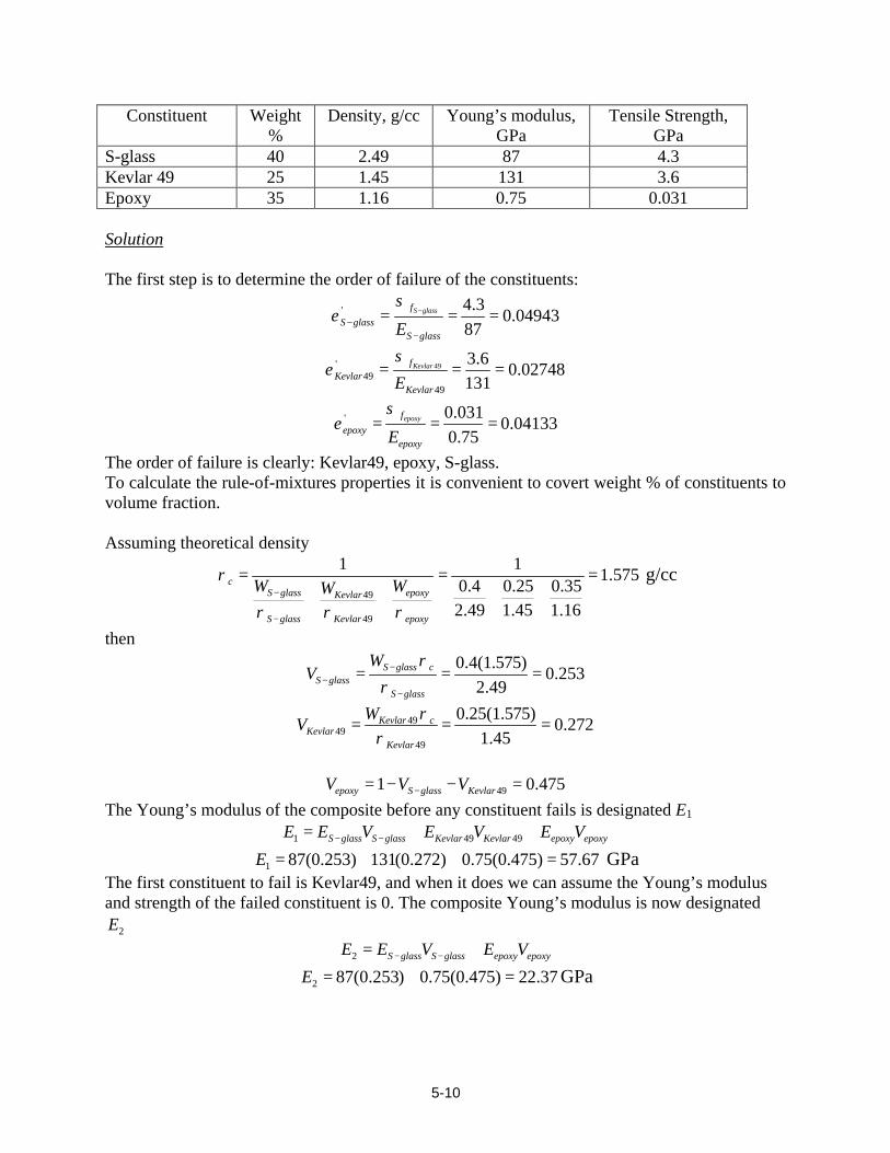
Constituent Weight %

Density, g/cc Young’s modulus, GPa

Tensile Strength, GPa

S-glass 40 2.49 87 4.3 Kevlar 49 25 1.45 131 3.6 Epoxy 35 1.16 0.75 0.031 Solution The first step is to determine the order of failure of the constituents:

' 4.30.04943

87S glassf

S glassS glassE

σε −

−−

= = =

49'49

49

3.60.02748

131Kevlarf

KevlarKevlarE

σε = = =

' 0.0310.04133

0.75epoxyf

epoxyepoxyE

σε = = =

The order of failure is clearly: Kevlar49, epoxy, S-glass. To calculate the rule-of-mixtures properties it is convenient to covert weight % of constituents to volume fraction. Assuming theoretical density

49

49

1 11.575

0.4 0.25 0.352.49 1.45 1.16

cS glass epoxyKevlar

S glass Kevlar epoxy

W WWρ

ρ ρ ρ−

−

= = =+ ++ +

g/cc

then

0.4(1.575)0.253

2.49S glass c

S glassS glass

WV

ρ

ρ−

−−

= = =

4949

49

0.25(1.575)0.272

1.45Kevlar c

KevlarKevlar

WV

ρρ

= = =

491 0.475epoxy S glass KevlarV V V−= − − =

The Young’s modulus of the composite before any constituent fails is designated E1 1 49 49S glass S glass Kevlar Kevlar epoxy epoxyE E V E V E V− −= + + 1 87(0.253) 131(0.272) 0.75(0.475) 57.67E = + + = GPa The first constituent to fail is Kevlar49, and when it does we can assume the Young’s modulus and strength of the failed constituent is 0. The composite Young’s modulus is now designated

2E 2 S glass S glass epoxy epoxyE E V E V− −= + 2 87(0.253) 0.75(0.475) 22.37E = + = GPa

5-11

The composite has a Young’s modulus, 3E when the epoxy fails 3 S glass S glassE E V− −= 3 87(0.253)E = GPa We can now construct the hypothetical stress-strain diagram, shown in Fig.5-4, using the failure strain and composite Young’s modulus calculated. The slope of the stress-strain curve is initially

1E . The stress at which the first constituent fails is '

1 1 49 57.67(0.02748) 1.585KevlarEσ ε= = = GPa after which the stress will drop immediately to '

1σ given by '

1 2 49 22.37(0.02748) 0.615KevlarEσ ε= = = GPa The slope of the stress-strain curve is now 2E . The stress at which the epoxy fails is '

2 2 22.37(0.04133) 0.9246epoxyEσ ε= = = GPa Since the epoxy is so weak there will now be a very slight stress drop to '

2 3 22.01(0.04133) 0.9097epoxyEσ ε= = = GPa The stress now rises with a slope of 3E to the failure strain of the S-glass

'3 3 22.01(0.04911) 1.081S glassEσ ε −= = = GPa

0

0.2

0.4

0.6

0.8

1

1.2

1.4

1.6

1.8

0 0.01 0.02 0.03 0.04 0.05 0.06

Strain

Str

ess,

GP

a

Figure 5-5 Stress-strain diagram for hybrid composite of Example Problem

5-12

Brittle matrix and ductile fiber with different failure strains Steel bar reinforced concrete is a good example of a composite with a brittle matrix and a ductile fiber. This composite is represented in Fig. 5-6. In this case the matrix fails before the fiber, therefore the stress on the fiber at matrix failure is

' 'f f mEσ ε=

At the lower fiber fractions the composite fails when the matrix fails and composite strength is given by the rule-of-mixture with the fiber contribution determined by '

fσ

' (1 )cu f f mu fV Vσ σ σ= + − (5.13)

0 1.0

FIBER FRACTIONSTRAIN

ε'm

ST

RE

SS

Vtrans

σmu

fuσ

fσ '

matrix

fiber

Figure 5-6 Stress-strain behavior for brittle matrix and ductile fiber At high fiber fraction the matrix can fail completely with the fibers holding the fractured matrix fragments in place and the composite strength is cu fu fVσ σ= (5.14)

The transition from matrix-dominated to fiber-dominated failure is referred to as transV . Is found by equating Eqn. (5.13) and Eqn.(5.14) and solving for fV

'mu

transfu mu f

Vσ

σ σ σ=

+ −

For f transV V> the matrix may split into a series of slabs held in place by the fibers as illustrated in Fig.5-7. Careful examination of the matrix slabs will reveal that they range in thickness between a characteristic value X’ and 2X’. This characteristic distance x’ can be determined by the force exerted by the fiber on the matrix parallel to the plane on the slab. Consider an elemental strip dx in the slab thickness, illustrated in Fig. 5-8. The force on the matrix, md Vσ is transferred from the fiber by shear around the cylinder of contact, 2 rdxπ ,by the fiber of radius r, hence

5-13

22 fm

Vd V rdx

rσ π τ

π= ⋅ ⋅ (5.15)

where the term, 2fV

rπ, is the total number of fibers.

FIBER

MATRIX

2x'

x'

Figure 5-7 Schematic diagram of slab formation in a brittle matrix, ductile fiber composite

d x

r

FIBER

MATRIX

Figure 5-8 Model for calculating force on matrix to result in slab formation Solving Eqn. (5.15) for dx and integrating over the limits from 0 to the characteristic thickness, X’

'

0 02muX

m

f

V rdx d

V

σσ

τ=∫ ∫ (5.16)

evaluating Eqn.(5.16)

'

2m mu

f

V rX

Vσ

τ=

2X’ is then the minimum distance to transfer sufficient force from the fiber to the matrix to cause matrix fracture, thus creating a slab. If a slab is 4X’ when it fracture it will crate two slabs exactly 2X’ thick. When they break there will be 4 slabs X’ thick. If a slab is between 2X’ and 4X’ it will fracture into a slab between X’ and 2X’, thus accounting for the range of observed slab thickness. This process is seen schematically in Fig. 5-9.

5-14

4x' 2x' <4x'

MA

TR

IX

ST

RE

SS

MA

TR

IX

ST

RE

SS

2x' x' <2x' Figure 5-9. Schematic diagram showing slab formation. It is apparent that if all the slabs we X’ thick the total strain would be less than if they ended up 2X’ thick. These two conditions would represent the extremes in possible strains. The maximum strain s can be determined by considering the fiber displacement. If the original slabs are all 2X’ thick before final fracture the maximum strain range is

max 1 m mmu

f f

V EV E

ε ε

∆ = −

(5.17)

If the original slabs are all 4X’ thick before final fracture the maximum strain range is

max 12

m mmu

f f

V EV E

ε ε

∆ = −

(5.18)

Most likely the average slab thickness would be a be between 2X’ and 4X’ thick, hence so the maximum strain will be between Eqns. (5.17) and (5.18). The representative resulting stress-strain diagram is illustrated in Fig. 5-10.

STRAIN

ST

RE

SS

Slabing phenomenonin matrix

Slope = V f E

mu maxεε

f

∆εmax

Figure 5-10. Stress-strain diagram for brittle matrix-ductile fiber composite exhibiting slabing.

5-15

TRANSVERSE PROPERTIES Transverse properties refer to properties of the composite in the direction normal to, as opposed to parallel to, the fibers as seen in Fig.5-11. The arrangement of constituents with respect to load direction are seen to be connected in series, as opposed to the constituent loaded in the longitudinal direction which can be considered connected in parallel.

L,1

T,2

S,3

MATRIX

FIBER

Load

Figure 5-11. Transverse loading of a composite. The slab model The analysis of the transverse loading is difficult because the relative amounts of constituent parallel to the load changes with distance along the T direction. Thus the strain in any plane, LS is different form any other plane if the fiber spacing is random. This is in contrast with the longitudinal case where any cross section normal to the load is identical to any other cross section even if the fiber spacing is random. To avoid the analytical complexity of a real composite, a hypothetical composite is considered in which the reinforcement phase and the matrix phase are alternated in the direction parallel to the load. Thus in any plane normal to the load either only matrix or only reinforcement is present. In this case the reinforcements are slabs not fibers. This model, which we may call the ‘slab’ model is depicted in Fig.5-12, and contains one reinforcement layer, sandwiched between two matrix layers. The total thickness of the composite is ct , the reinforcement thickness is ft , and the matrix thickness is mt . In this model

the elongation of the composite, cδ is the sum of the reinforcement elongation, fδ and the

matrix elongation, mδ . Expressing the elongations in terms of strain and thickness c c f f m mt t tε ε ε= + (5.19)

Dividing both sides of Eqn.(5.19) by ct results in the composite strain

f f m mc

c c

t tt t

ε εε = + (5.20)

Recognizing that f ct t and m ct t are the reinforcement volume fraction and matrix volume fractions respectively, Eqn. (5.20) can be written (1 )c f f m fV Vε ε ε= + − (5.21)

5-16

Thus the composite strain in the transverse slab model appears to follow the simple rule-of-mixtures.

tftm/2 tm/2

matrix

reinforcement

Longitudinal

Transverse

Figure 5-12 Slab model of a composite to analyze transverse behavior. Since the constituents of the slab model are arranged in series it is obvious that loads in the constituents and composite are equal, thus c f mP P P= = (5.22) In this model the area normal to the loading direction is also equal therefore the stresses in the constituents are also equal, c f mσ σ σ= = (5.23) Writing Eqn.(5.21) in terms of stress and modulus and using Eqn.(5.23)

fT

m f m m f

EEE V E V E

=+

(5.24)

5-17

The transverse Young’s modulus determines using the slab model is compared to the longitudinal Young’s modulus normalized by the matrix modulus over the range of fiber volume fractions is shown in Fig. 5-13.

0 0.25 0.50 0.75 1.0

10

8

6

4

2

0

Fiber Volume Fraction , Vf

E T /

Em

Longitudinal(Parallel Connected)

Transverse(Serial Connected)

Figure 5-13. Comparison of transverse (Slab Model) and longitudinal Young’s modulus Compared to the longitudinal Young’s modulus the transverse modulus is significantly lower. Increasing fiber volume fraction has only a modest effect on increasing transverse stiffness at fiber fractions below 0.75. At higher volume fractions the transverse stiffness begins to increase rapidly, however there are practical limitations to the achieving fiber fractions above 0.75 in most composites. The limitations in fiber volume fraction are discussed in the Addendum to this chapter. The slab model has a number of very serious limitations, not the least of which is that it does not represent many common composites. Figure 5-14a is more representative than Fig. 5-14b of most composites. In a realistic model both reinforcement and matrix are present in any cross section. In the slab model either matrix or reinforcement is present.

a) realistic model b) slab model Figure 5-14. Comparison of slab model and realistic composites.

5-18

Elasticity model In a realistic model the arrangement of the reinforcement will influence the transverse stiffness as well as other properties. Since the actual arrangement for reinforcements cannot be known precisely some method must be devised to approximately describe it. For this purpose one can use models of fiber contiguity shown in Fig.5-15. If round fibers have the maximum number of neighbors touching them the contiguity value, C is 1. If no fibers are touching the contiguity value C = 0. Most composites have partial contiguity, therefore 0 1C < < .

C= 0 C=1

ISOLATED MATRIXFIBERS CONTIGUOUS

ISOLATED FIBERSMATRIX CONTIGUOUS

0<C<1

PARTIAL CONTIGUITY

Figure 5-15 Contiguity models for calculating transverse elastic properties. The transverse Young’s modulus base on an elasticity solution using the contiguity models is given as

( )( )

( ) ( )( ) ( )

( ) ( )( ) ( )

21

2 22 1

2

2 2

f m m m f m m

m m f m m

T f f m m

f m f f m f m

m f m f m

K K G G K K VC

K G K K VE V

K K G G K K VC

K G K K V

ν ν ν

+ − −− +

+ + − = − + − + + −

+ − −

(5.25)

where ( )2 1

ff

f

EK

ν=

−,

( )2 1m

mm

EK

ν=

−,

( )2 1f

ff

EG

ν=

+, and

( )2 1m

mm

EG

ν=

+

The shear modulus is given as

( ) ( )( )

( ) ( )( ) ( )

21

2f f m m f m f m m

L m fm f m m f m f m m

G G G V G G G G VG C G CG

G G G V G G G G V

− − + − −= − +

+ − + + −

The Poisson’s ratio is

( )( ) ( )

( ) ( )( ) ( )

( ) ( )2 2 2 2

12 2

f f m m m m m f m m m m f f m f f m f fLT

f m m m f m m f m m f m f m

K K G V K K G V K K G V K K G VC C

K K G G K K V K K G G K K V

ν ν ν νν

+ + + + + += − +

+ − − + + −

5-19

Halpin-Tsai Equations The slab model for transverse elastic modulus uses assumptions that are clearly rarely achieved in realistic composites while the elasticity solution utilizing contiguity models, requires an accurate value for C which are not easily determined. This has lead to a semi-empirical approach known as the Halpin-Tsai equations. For transverse Young’s modulus

1

1fT

m f

VEE V

ξη

η

+=

− (5.26)

where

1f

m

f

m

EEEE

ηξ

−=

+ (5.27)

and

( )2 abξ =

The ratio ab is the cross sectional aspect ratio of the reinforcement as defined in Fig.5-16.

a

b

b

LOADLOAD

Figure 5-16 Cross sectional aspect ratio of reinforcement in the definition of ξ . The a direction is always defined as the dimension of the reinforcement in the direction of loading. The b direction is transverse to the load. When the Halpin-Tsai equation is used to determine the shear modulus LTG then

1.732

ab

ξ =

Consider a rectangular cross section reinforcement as illustrated in Fig. 5-17.

5-20

STRESSSTRESS

ba

Figure 5-17 A representation of a rectangular cross section reinforcement For the case of 0ξ = then 2 0a

b = , hence 0a → and b → ∞ and the arrangement of the

reinforcement in the composite is now represented by Fig. 5-18.

STRESSSTRESS

a

b

Figure 5-18 The reinforcement shape for the case of 0ξ = . It can be seen that Fig. 5-18 is in appearance the slab model for transverse properties. Substituting 0ξ = into Eqn.(5.26)

11

T

m f

EE Vη

=−

(5.28)

and

f m

f

E E

Eη

−= (5.29)

Combining Eqns. (5.28) an (5.29)

fT

m f m m f

EEE V E V E

=+

(5.30)

The results are identical to Eqn. (5.24) for the serially connected constituent or slab model. For the case of ξ = ∞ , then a → ∞ and 0b → . The arrangement of the reinforcement is now illustrated in Fig.5-19. This is now the slab model for parallel connected constituents. Substituting ξ = ∞ into Eqn.(5.26)

1

1fT

m f

VEE V

η

η

+ ∞=

− (5.31)

and

5-21

f m

m

E E

Eη

−=

∞ (5.32)

Combining Eqns. (5.31) an (5.32) T f f m mE E V E V= + (5.33)

STRESSSTRESS b

a

Figure 5.19. Reinforcement shape for ξ = ∞ . Eqn.(5.33) is the form of the equation for longitudinal Young’s modulus based on the rule-of -mixtures for parallel connected constituents. Fig. 5-20 is a plot comparing the three methods of predicting the transverse Young’s modulus over the range of fiber fractions. The three values of contiguity: 0C = , 0.5C = and 1C = , represent the limits and an average value. The slab model predicts the lowest value of Young’s modulus while the elastic model with 1C = has the greatest. The Halpin-Tsai and the elastic model, 0.5C = lie within these limits.

0.0

10.0

20.0

30.0

40.0

50.0

60.0

70.0

80.0

90.0

100.0

0 0.1 0.2 0.3 0.4 0.5 0.6 0.7 0.8 0.9 1

Volume Fraction, Vf

Tra

nsv

erse

Yo

un

g's

Mo

du

lus

Slab ModelHalpin-TsaiElastic C=0Elastic C=0.5Elastic C=1

Figure 5-20. Comparison of transverse Young’s modulus determined by three methods

5-22

Transverse tensile strength The transverse tensile strength of a composite is most likely less than the strength of the matrix alone. The fibers will act as stress concentrations, increasing the local stress in the material. Defects in fiber-matrix bond interface can be sufficiently large to constitute critical flaws. The transverse strength can be expressed as

muTU S

σσ = (5.34)

where S is called the strength reduction factor. The approach to determining the value of S uses either analytical or empirical estimates for the transverse composite failure strain, *

Tε . Using the analytical estimate

1/ 2

* 41 1f m

T muf

V EE

ε επ

= − −

(5.35)

Assuming brittle fracture

* TUT

TEσ

ε = (5.36)

and

mumu

mEσ

ε = (5.37)

Combining Eqns.(5.35) ,(5.36) and (5.37) gives

1/ 241 1f m

T muf

TUm

V EE

E

E

σπ

σ

− − = (5.38)

Using the empirical relation ( )* 1/31T mu fVε ε= − (5.40)

Combining Eqns.(5.40), (5.36) and (5.37) gives

( )1/ 31T mu f

TUm

E V

E

σσ

−= (5.41)

Any of the three methods discussed above can be used to determine TE . However, since TE is also a function of fiber fraction, the value of fV in Eqn.5.41 must be the same as was used to

calculate TE .

5-23

Using the Halpin-Tsai method for evaluating transverse strength, Eqn.5.41 can be written as

( )1/3

11

11

1

F

mf

F

m muTU m f

F m

mf

F

m

EE

VEE

E VE EE

VEE

− + ξ + ξ σ σ = − −

− + ξ

(5.42)

which simplifies to

( ) ( )( )

1/ 3 1fTU f m f f f m mu

f m f f f m

VE E V E V E

E E V E V E

−σ = + ξ + ξ − ξ σ

− − ξ + − (5.43)

Figure 5.21 is a plot of transverse strength versus fiber volume fraction using the Halpin-Tsai estimate for transverse Young’s Modulus. For this plot S-glass is used as the fiber in a rigid epoxy matrix.

For this composite a local minimum exists at about 20% fiber content and a local maximum occurs at just over 50% fiber content, High transverse strength can be achieved over a broad range of fiber content but drops off abruptly at fiber fractions above 0.70. The transverse Young’s Modulus on the other hand is low over the range from 0 to 0.70 fiber fraction and rapidly increases above 0.70 fiber content, as can be seen in Figure 5.22

This interaction makes it difficult to design composites which are both stiff and strong in the transverse direction. This is the principal reason for forming composites with fibers oriented in more than one direction. The exact form of the transverse strength- fiber fraction curve depends upon the properties of the constituents. The strength curve for a metal matrix composite consisting of SiC monofilament fibers in magnesium alloy matrix is shown in Figure 5.23. For this case there are no local minima or maxima in the transverse strength versus fiber fraction curve. The transverse Young’s Modulus versus fiber fraction plot in Figure 5.24 has a less pronounced rise at the highest fiber fractions. This transverse strength estimate is based on the assumption that matrix strength controls the transverse fracture strength and the bonding between the fiber and matrix is strong. For weakly bonded fibers the interfacial strength controls fracture and length of weakly bonded or unbonded fibers normal to the load will determine transverse strength. In these cases fracture mechanics methods may be appropriate. If the fibers have poor transverse strength, such as high modulus carbon fibers and Kevlar fibers, then Eqns. 5.41 to 5.43 do not apply.

5-24

0

10

20

30

40

50

60

0.00 0.10 0.20 0.30 0.40 0.50 0.60 0.70 0.80 0.90 1.00

Volume Fraction Fiber

Tra

nsv

erse

Str

eng

th, M

Pa

Figure 5.21 Variation in transverse strength with fiber fraction for S-Glass/epoxy composite.

0

10

20

30

40

50

60

70

80

90

100

0.00 0.10 0.20 0.30 0.40 0.50 0.60 0.70 0.80 0.90 1.00

Volume Fraction Fiber

Tra

nsv

erse

Yo

un

g's

Mo

du

lus,

GP

a

Figure 5.22 Transverse Young’s Modulus as a function of fiber fraction for S-Glass/epoxy composite as determined by Halpin-Tsai method.

5-25

0.0

25.0

50.0

75.0

100.0

125.0

150.0

175.0

200.0

225.0

250.0

0.00 0.10 0.20 0.30 0.40 0.50 0.60 0.70 0.80 0.90 1.00

Volume Fraction Fiber

Tra

nsv

erse

Str

eng

th, M

Pa

Figure 5.23 Variation in transverse strength with fiber fraction for SiC monofilament/Mg Alloy composite

0.0

50.0

100.0

150.0

200.0

250.0

300.0

350.0

400.0

450.0

0.00 0.10 0.20 0.30 0.40 0.50 0.60 0.70 0.80 0.90 1.00

Volume Fraction Fiber

Tra

nsv

erse

Yo

un

g's

Mo

du

lus,

GP

a

. Figure 5.24 Transverse Young’s Modulus as a function of fiber fraction for SiC monofilament/Mg Alloy composite as determined by Halpin -Tsai method

5-26

Example Problem 5.2 Calculate the volume fraction of fibers necessary to produce a transverse strength of 0.050 GPa if the transverse Young’s Modulus of the composite , ET , is 13.298 GPa and the matrix have the following properties: Em = 3.1 GPa and σmu=0.072 GPa. Solution The transverse strength can be found form the empirical equation (Eqn. 5.14)

( )1/ 31T mu f

TUm

E V

E

−=

σσ

Solving for Vf

3

3

1

3.1(0.051)1

13.298(0.072)

0.58

m TUf

T mu

f

f

EV

E

V

V

σ= − σ

= −

=

5-27

Addendum to Chapter 5

Limitations to volume fraction In the fabrication of composites there are both theoretical and practical limitation to the amount of fibers that can be incorporated. The packing of the fibers is one such limitation. Packing or ability for the fibers to fit geometrically in a given space depends upon the shape and size of the fiber. Fine diameter fibers are more difficult to pack than large diameter fibers. Large diameter fibers can be nested individually so that they fit neatly in the groove formed by the previous layer. Hence monofilaments can be filament wound to near theoretical packing density. Some examples of fiber packing geometry are shown in Fig.5-21.

Square Array Close Packing

Random Regular Open

Figure 5.21 Example of fiber packing Many manufactured fibers are not perfectly straight or for that matter have uniform geometry. They can have bends, twists and kink. These defects will result in the fibers touching at points rather than along their entire length thus adding unwanted matrix volume. Finally, during the introduction of the resin or other matrix material the fibers can undergo spontaneous separation due to high surface tension. This phenomenon will tend to reduce the fibers geometric density. Each packing geometry has a unique theoretical density. For the square array shown in Fig. 5.22 the maximum fiber volume fraction

maxfV is the area of the fiber within the unit cell area of the composite

max

2

2

40.785f

D

VD

π = =

5-28

D

Figure 5.22 Fibers in square array packing For the close packed array shown in Fig. 5.23

max

4

28 0.907

34

f

D

VD

π

= =

D

Figure 5.23 Fibers in closed packed array

5-29

Example Problem 5.3 You are designing a structure for operation at 750°F using boron fibers and polyamide-imide matrix. This structure must meet the following room temperature requirements:

1

2

35,000,000 psi

7,000,000 psi

E

E

==

What percent by volume of boron fibers would you require, assuming that the boron fibers have a Young’s Modulus of 57,000,000 psi and the resin has a Young’s Modulus of 720,000 psi? Solution To meet the longitudinal stiffness requirements the parallel connected rule-of-mixtures predicts

1

1

(1 )

35,000,000 720,0000.609

57,000,000 720,000

f f m f

mf

f m

f

E E V E V

E EV

E E

V

= + −

−=

−

−= =

−

Fiber volume is 60.9% to achieve E1=35,000,000 psi The transverse Young’s Modulus, E2, can be determined using the “Slab Model” of serially connected constituents

2

2

2

(1 )

( )

( )

57,000,000(720,000 7,000,000)7,000,000(720,000 57,000,000

0.909

f m

m f f f

f mf

m f

f

f

E EE

E V E V

E E EV

E E E

V

V

=+ −

−=

−

−=

−=

The fiber volume is 90.9% to achieve E2 = 7,000,000 psi. However the maximum theoretical packing density allows a maximum of only 90.6% fibers. In fact the practical limit is probably closer to 85% fibers, hence the required transverse modulus cannot be achieved with the fiber selected. The Slab Model however significantly under-predicts the transverse Young’s Modulus, especially at high volume fractions of fibers. A better estimate of the transverse elastic modulus would be obtained using the Halpin-Tsai method.

5-30

2

(1 )

(1 )

1

m f

f

f

m

f

m

E VE

V

EEEE

ηξ

η

ηξ

+=

−

−=

+

Solving for Vf

2

2

mf

m

E EV

E Eξ ηξ−

=+

For circular cross-sectioned fibers, 2ξ =

57,000,0001

720,000 0.96357,000,000

2720,000

7,000,000 720,0000.773

7,000,000(0.963) 720,000(0.963)(2)fV

η−

= =+

−= =

+

This estimate of 77.3 % by volume, is well within the range of reasonably obtained fiber contents that can be produced by filament winding of mono-filaments.