6entropy & the boltzmann law - brandeis university2004-9-29 · 6entropy & the boltzmann...

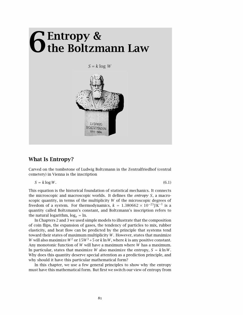
6Entropy &the Boltzmann Law

S = k log W

What Is Entropy?

Carved on the tombstone of Ludwig Boltzmann in the Zentralfriedhof (centralcemetery) in Vienna is the inscription

S = k logW. (6.1)

This equation is the historical foundation of statistical mechanics. It connectsthe microscopic and macroscopic worlds. It defines the entropy S, a macro-scopic quantity, in terms of the multiplicity W of the microscopic degrees offreedom of a system. For thermodynamics, k = 1.380662 × 10−23J K−1 is aquantity called Boltzmann’s constant, and Boltzmann’s inscription refers tothe natural logarithm, loge = ln.

In Chapters 2 and 3 we used simple models to illustrate that the compositionof coin flips, the expansion of gases, the tendency of particles to mix, rubberelasticity, and heat flow can be predicted by the principle that systems tendtoward their states of maximum multiplicityW . However, states that maximizeW will also maximizeW 2 or 15W 3+5 or k lnW , where k is any positive constant.Any monotonic function of W will have a maximum where W has a maximum.In particular, states that maximize W also maximize the entropy, S = k lnW .Why does this quantity deserve special attention as a prediction principle, andwhy should it have this particular mathematical form?

In this chapter, we use a few general principles to show why the entropymust have this mathematical form. But first we switch our view of entropy from

81

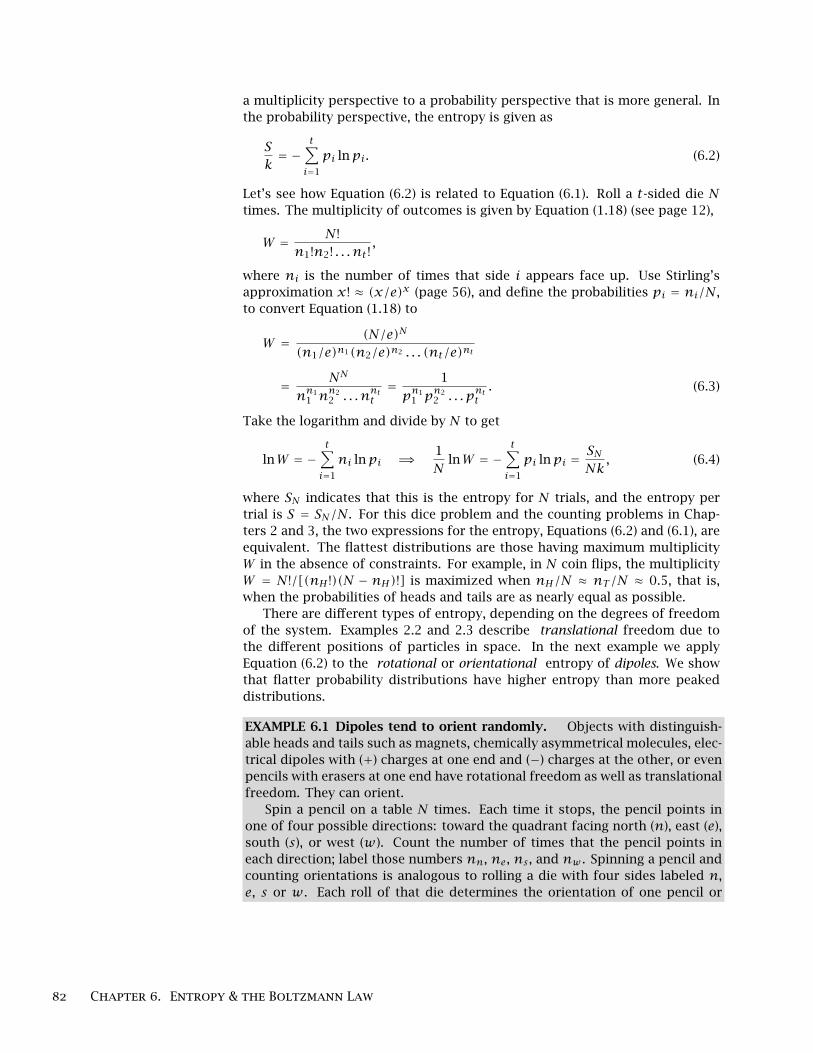
a multiplicity perspective to a probability perspective that is more general. Inthe probability perspective, the entropy is given as

Sk= −

t∑i=1

pi lnpi. (6.2)

Let’s see how Equation (6.2) is related to Equation (6.1). Roll a t-sided die Ntimes. The multiplicity of outcomes is given by Equation (1.18) (see page 12),

W = N !n1!n2! . . . nt !

,

where ni is the number of times that side i appears face up. Use Stirling’sapproximation x! ≈ (x/e)x (page 56), and define the probabilities pi = ni/N ,to convert Equation (1.18) to

W = (N/e)N

(n1/e)n1(n2/e)n2 . . . (nt/e)nt

= NN

nn11 n

n22 . . . nntt

= 1

pn11 p

n22 . . . pntt

. (6.3)

Take the logarithm and divide by N to get

lnW = −t∑i=1

ni lnpi �⇒ 1N

lnW = −t∑i=1

pi lnpi = SNNk

, (6.4)

where SN indicates that this is the entropy for N trials, and the entropy pertrial is S = SN/N . For this dice problem and the counting problems in Chap-ters 2 and 3, the two expressions for the entropy, Equations (6.2) and (6.1), areequivalent. The flattest distributions are those having maximum multiplicityW in the absence of constraints. For example, in N coin flips, the multiplicityW = N !/[(nH !)(N − nH)!] is maximized when nH/N ≈ nT/N ≈ 0.5, that is,when the probabilities of heads and tails are as nearly equal as possible.

There are different types of entropy, depending on the degrees of freedomof the system. Examples 2.2 and 2.3 describe translational freedom due tothe different positions of particles in space. In the next example we applyEquation (6.2) to the rotational or orientational entropy of dipoles. We showthat flatter probability distributions have higher entropy than more peakeddistributions.

EXAMPLE 6.1 Dipoles tend to orient randomly. Objects with distinguish-able heads and tails such as magnets, chemically asymmetrical molecules, elec-trical dipoles with (+) charges at one end and (−) charges at the other, or evenpencils with erasers at one end have rotational freedom as well as translationalfreedom. They can orient.

Spin a pencil on a table N times. Each time it stops, the pencil points inone of four possible directions: toward the quadrant facing north (n), east (e),south (s), or west (w). Count the number of times that the pencil points ineach direction; label those numbers nn, ne, ns , and nw . Spinning a pencil andcounting orientations is analogous to rolling a die with four sides labeled n,e, s or w. Each roll of that die determines the orientation of one pencil or

82 Chapter 6. Entropy & the Boltzmann Law

(a) Ordered (b) Biased (d) Random(c) Biased

pi

n e s w

1

0 0 0

n e s w

14

14

14

14

0 0

n e s w

12

12

n e s w

16

16

13

13

Figure 6.1 Spin a hundred pencils. Here are four (of a large number) of possibledistributions of outcomes. (a) All pencils could point north (n). This is the mostordered distribution, S/k = −1 ln 1 = 0. (b) Half the pencils could point east (e) andhalf could point south (s). This distribution has more entropy than (a),S/k = −2(1/2 ln 1/2) = 0.69. (c) One-third of the pencils could point n, and one-thirdw, one-sixth e, and one-sixth s. This distribution has even more entropy,S/k = −2(1/3 ln 1/3+ 1/6 ln 1/6) = 1.33. (d) One-quarter of the pencils could point ineach of the four possible directions. This is the distribution with highest entropy,S/k = −4(1/4 ln 1/4) = 1.39.

dipole. N die rolls correspond to the orientations of N dipoles. The numberof configurations for systems with N trials, distributed with any set of out-comes {n1, n2, . . . , nt}, where N = ∑t

i=1ni, is given by the multiplicity Equa-tion (1.18): W(n1, n2, . . . , nt) = N !/(n1!n2! · · ·nt !). The number of differentconfigurations of the system with a given composition nn, ne, ns , and nw is

W(N,nn,ne,ns,nw) = N !nn!ne!ns !nw !

.

The probabilities that a pencil points in each of the four directions are

p(n) = nnN, p(e) = ne

N, p(s) = ns

N, and p(w) = nw

N.

Figure 6.1 shows some possible distributions of outcomes. Each distributionfunction satisfies the constraint that p(n) + p(e) + p(s) + p(w) = 1. Youcan compute the entropy per spin of the pencil of any of these distributionsby using Equation (6.2), S/k = −∑t

i=1 pi lnpi. The absolute entropy is nevernegative, that is S ≥ 0.

Flat distributions have high entropy. Peaked distributions have low entropy.When all pencils point in the same direction, the system is perfectly orderedand has the lowest possible entropy, S = 0. Entropy does not depend on beingable to order the categories along an x-axis. For pencil orientations, there is nodifference between the x-axis sequence news and esnw. To be in a state of lowentropy, it does not matter which direction the pencils point in, just that they allpoint the same way. The flattest possible distribution has the highest possibleentropy, which increases with the number of possible outcomes. In Figure 6.1we have four states: the flattest distribution has S/k = −4(1/4) ln(1/4) =ln 4 = 1.39. In general, when there are t states, the flat distribution has entropyS/k = ln t. Flatness in a distribution corresponds to disorder in a system.

What Is Entropy? 83

The concept of entropy is broader than statistical thermodynamics. It is aproperty of any distribution function, as the next example shows.

p

w g bl r brColor

110

110

210

310

310

Figure 6.2 The entropy canbe computed for anydistribution function, evenfor colors of socks: white(w), green (g), black (bl),red (r ), and brown (br ).

EXAMPLE 6.2 Colors of socks. Suppose that on a given day, you sample 30students and find the distribution of the colors of the socks they are wearing(Figure 6.2). The entropy of this distribution is

S/k = −0.2 ln 0.2− 0.6 ln 0.3− 0.2 ln 0.1 = 1.50.

For this example and Example 6.1, k should not be Boltzmann’s constant. Boltz-mann’s constant is appropriate only when you need to put entropy into unitsthat interconvert with energy, for thermodynamics and molecular science. Forother types of probability distributions, k is chosen to suit the purposes athand, so k = 1 would be simplest here. The entropy function just reports therelative flatness of a distribution function. The limiting cases are the most or-dered, S = 0 (everybody wears the same color socks) and the most disordered,S/k = ln t = ln 5 = 1.61 (all five sock colors are equally likely).

Why should the entropy have the form of either Equation (6.1) or Equation(6.2)? Here is a simple justification. A deeper argument is given in ‘OptionalMaterial,’ page 89.

The Simple Justification for S = k lnW

Consider a thermodynamic system having two subsystems,A and B, with multi-plicitiesWA andWB respectively. The multiplicity of the total system will be theproduct Wtotal = WAWB . Thermodynamics requires that entropies be extensive,meaning that the system entropy is the sum of subsystem entropies, Stotal =SA + SB . The logarithm function satisfies this requirement. If SA = k lnWA andSB = k lnWB , then Stotal = k lnWtotal = k lnWAWB = k lnWA + k lnWB = SA + SB .This argument illustrates why S should be a logarithmic function of W .

Let’s use S/k = −∑i pi lnpi to derive the exponential distribution law,called the Boltzmann distribution law, that is at the center of statistical thermo-dynamics. The Boltzmann distribution law describes the energy distributionsof atoms and molecules.

Underdetermined Distributions

In the rest of this chapter, we illustrate the principles that we need by concoct-ing a class of problems involving die rolls and coin flips instead of molecules.How would you know if a die is biased? You could roll it N times and count thenumbers of 1’s, 2’s, …, 6’s. If the probability distribution were perfectly flat,the die would not be biased. You could use the same test for the orientations ofpencils or to determine whether atoms or molecules have biased spatial orien-tations or bond angle distributions. However the options available to moleculesare usually so numerous that you could not possibly measure each one. In sta-tistical mechanics you seldom have the luxury of knowing the full distribution,corresponding to all six numbers pi for i = 1,2,3, . . . ,6 on die rolls.

Therefore, as a prelude to statistical mechanics, let’s concoct dice prob-lems that are underdetermined in the same way as the problems of molecular


science. Suppose that you do not know the distribution of all six possible out-comes. Instead, you know only the total score (or equivalently, the averagescore per roll) on the N rolls. In thousands of rolls, the average score per rollof an unbiased die will be 3.5 = (1 + 2 + 3 + 4 + 5 + 6)/6. If you observe thatthe average score is 3.5, it is evidence (but not proof)1 that the distribution isunbiased. In that case, your best guess consistent with the evidence is that thedistribution is flat. All outcomes are equally likely.

However, if you observe the average score per roll is 2.0, then you must con-clude that every outcome from 1 to 6 is not equally likely. You know only thatlow numbers are somehow favored. This one piece of data—the total score—isnot sufficient to predict all six unknowns of the full distribution function. Sowe aim to do the next best thing. We aim to predict the least biased distributionfunction that is consistent with the known measured score. This distributionis predicted by the maximum-entropy principle.

Maximum Entropy Predicts Flat DistributionsWhen There Are No Constraints

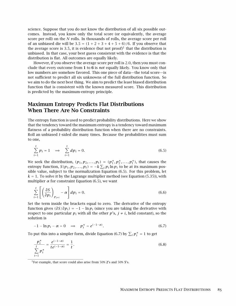
The entropy function is used to predict probability distributions. Here we showthat the tendency toward the maximum entropy is a tendency toward maximumflatness of a probability distribution function when there are no constraints.Roll an unbiased t-sided die many times. Because the probabilities must sumto one,

t∑i=1

pi = 1 �⇒t∑i=1

dpi = 0. (6.5)

We seek the distribution, (p1, p2, . . . , pt) = (p∗1 , p∗2 , . . . , p

∗t ), that causes the

entropy function, S(p1, p2, . . . , pt) = −k∑i pi lnpi to be at its maximum pos-

sible value, subject to the normalization Equation (6.5). For this problem, letk = 1. To solve it by the Lagrange multiplier method (see Equation (5.35)), withmultiplier α for constraint Equation (6.5), we want

t∑i=1

( ∂S∂pi

)pj≠i

−αdpi = 0. (6.6)

Set the term inside the brackets equal to zero. The derivative of the entropyfunction gives (∂S/∂pi) = −1 − lnpi (since you are taking the derivative withrespect to one particular pi with all the other p’s, j ≠ i, held constant), so thesolution is

−1− lnpi −α = 0 �⇒ p∗i = e(−1−α). (6.7)

To put this into a simpler form, divide Equation (6.7) by∑i p∗i = 1 to get

p∗it∑i=1

p∗i

= e(−1−α)

te(−1−α) =1t. (6.8)

1For example, that score could also arise from 50% 2’s and 50% 5’s.

Maximum Entropy Predicts Flat Distributions 85

Maximizing the entropy predicts that when there is no bias, all outcomes areequally likely. However, what if there is bias? The next section shows howmaximum entropy works in that case.

Maximum Entropy Predicts Exponential DistributionsWhen There Are Constraints

Roll a die having t sides, with faces numbered i = 1,2,3, . . . , t. You do not knowthe distribution of outcomes of each face, but you know the total score after Nrolls. You want to predict the distribution function. When side i appears faceup, the score is εi. The total score after N rolls will be E =∑t

i=1 εini, where niis the number of times that you observe face i. Let pi = ni/N represent thefraction of the N rolls on which you observe face i. The average score per roll〈ε〉 is

〈ε〉 = EN=

t∑i=1

piεi. (6.9)

What is the expected distribution of outcomes (p∗1 , p∗2 , . . . , p

∗t ) consistent

with the observed average score 〈ε〉? We seek the distribution that maximizesthe entropy, Equation (6.2), subject to two conditions: (1) that the probabilitiessum to one and (2) that the average score agrees with the observed value 〈ε〉,

g(p1, p2, . . . , pt) =t∑i=1

pi = 1 �⇒t∑i=1

dpi = 0, (6.10)

and

h(p1, p2, . . . , pt) = 〈ε〉 =t∑i=1

piεi �⇒t∑i=1

εidpi = 0. (6.11)

The solution is given by the method of Lagrange multipliers (pages 69–73):(∂S∂pi

)−α

(∂g∂pi

)− β

(∂h∂pi

)= 0 for i = 1,2, . . . , t, (6.12)

where α and β are the unknown multipliers. The partial derivatives are evalu-ated for each pi:(

∂S∂pi

)= −1− lnpi,

(∂g∂pi

)= 1, and

(∂h∂pi

)= εi. (6.13)

Substitute Equations (6.13) into Equation (6.12) to get t equations of the form

−1− lnp∗i −α− βεi = 0, (6.14)

where the p∗i ’s are the values of pi that maximize the entropy. Solve Equa-tions (6.14) for each p∗i :

p∗i = e(−1−α−βεi). (6.15)


To eliminate α in Equation (6.15), use Equation (6.10) to divide both sides byone. The result is an exponential distribution law:

p∗i =p∗it∑i=1

p∗i

= e(−1−α)e−βεit∑i=1

e(−1−α)e−βεi= e−βεi

t∑i=1

e−βεi. (6.16)

In statistical mechanics, this is called the Boltzmann distribution law and thequantity in the denominator is called the partition function q,

q =t∑i=1

e−βεi . (6.17)

Using Equations (6.11) and (6.16) you can express the average score per roll 〈ε〉(Equation (6.9)) in terms of the distribution,

〈ε〉 =t∑i=1

εip∗i =1q

t∑iεie−βεi . (6.18)

The next two examples show how Equation (6.18) predicts all t of the p∗i ’s fromthe one known quantity, the average score.

EXAMPLE 6.3 Finding bias in dice by using the exponential distribution law.Here we illustrate how to predict the maximum entropy distribution whenan average score is known. Suppose a die has t = 6 faces and the scoresequal the face indices, ε(i) = i. Let x = e−β. Then Equation (6.17) givesq = x + x2 + x3 + x4 + x5 + x6, and Equation (6.16) gives

p∗i =xi

6∑i=1

xi= xi

x + x2 + x3 + x4 + x5 + x6. (6.19)

From the constraint Equation (6.18), you have

〈ε〉 =6∑i=1

ip∗i =x + 2x2 + 3x3 + 4x4 + 5x5 + 6x6

x + x2 + x3 + x4 + x5 + x6. (6.20)

You have a polynomial, Equation (6.20), that you must solve for the one un-known x (a method for solving polynomials like Equation (6.20) is given onpage 55). You begin with knowledge of 〈ε〉. Compute the value x∗ that solvesEquation (6.20). Then substitute x∗ into Equations (6.19) to give the distribu-tion function (p∗1 , p

∗2 , . . . , p

∗t ).

For example, if you observe the average score 〈ε〉 = 3.5, then x = 1 satisfiesEquation (6.20), predicting p∗i = 1/6 for all i, indicating that the die is unbiasedand has a flat distribution (see Figure 6.3(a)).

If, instead, you observe the average score is 〈ε〉 = 3.0, thenx = 0.84 satisfiesEquation (6.20), and you have q = 0.84+0.842+0.843+0.844+0.845+0.846 =3.41. The probabilities are p1 = 0.84/3.41 = 0.25, p2 = 0.842/3.41 = 0.21,p3 = 0.843/3.41 = 0.17, and so on, as shown in Figure 6.3(b).

Maximum Entropy Predicts Exponential Distributions 87

1 2 3 4 5 6i

(a) 〈ε〉 = 3.5

0.167

1 2 3 4 5 6i

(b) 〈ε〉 = 3.0

0.250.21

0.170.15

0.12 0.10

1 2 3 4 5 6i

(c) 〈ε〉 = 4.0

0.250.21

0.170.15

0.120.10

pi pi

piFigure 6.3 The probabilities of diceoutcomes for known average scores.(a) If the average score per roll is〈ε〉 = 3.5, then x = 1 and all outcomesare equally probable, predicting thatthe die is unbiased. (b) If the averagescore is low (〈ε〉 = 3.0, x = 0.84),maximum entropy predicts anexponentially diminishingdistribution. (c) If the average score ishigh (〈ε〉 = 4.0, x = 1.19), maximumentropy implies an exponentiallyincreasing distribution.

If you observe 〈ε〉 < 3.5, then the maximum-entropy principle predicts anexponentially decreasing distribution (see Figure 6.3(b)), with more 1’s than2’s, more 2’s than 3’s, etc. If you observe 〈ε〉 > 3.5, then maximum entropypredicts an exponentially increasing distribution (see Figure 6.3(c)): more 6’sthan 5’s, more 5’s than 4’s, etc. For any given value of 〈ε〉, the exponentialor flat distribution gives the most impartial distribution consistent with thatscore. The flat distribution is predicted either if the average score is 3.5 or ifyou have no information at all about the score.

EXAMPLE 6.4 Biased coins? The exponential distribution again. Let’sdetermine a coin’s bias. A coin is just a die with two sides, t = 2. Score tailsεT = 1 and heads εH = 2. The average score per toss 〈ε〉 for an unbiased coinwould be 1.5.

Again, to simplify, write the unknown Lagrange multiplier β in the formx = e−β. In this notation, the partition function Equation (6.17) is q = x + x2.According to Equation (6.16), the exponential distribution law for this two-statesystem is

p∗T =x

x + x2and p∗H =

x2

x + x2. (6.21)


From the constraint Equation (6.18) you have

〈ε〉 = 1p∗T + 2p∗H =x + 2x2

x + x2= 1+ 2x

1+ x .

Rearranging gives

x = 〈ε〉 − 12− 〈ε〉 .

If you observe the average score to be 〈ε〉 = 1.5, then x = 1, and Equation (6.21)gives p∗T = p∗H = 1/2. The coin is fair. If instead you observed 〈ε〉 = 1.2, thenx = 1/4, and you have p∗H = 1/5 and p∗T = 4/5.

There are two situations that will predict a flat distribution function. First,it will be flat if 〈ε〉 equals the value expected from a uniform distribution. Forexample, if you observe 〈ε〉 = 3.5 in Example 6.3, maximum entropy predictsa flat distribution. Second, if there is no constraint at all, you expect a flatdistribution. By the maximum-entropy principle, having no information is thesame as expecting a flat distribution.

On page 84, we gave a simple rationalization for why S should be a logarith-mic function of W . Now we give a deeper justification for the functional form,S/k = −∑i pi lnpi. You might ask why entropy must be extensive, and whyentropy, which we justified on thermodynamic grounds, also applies to a broadrange of problems outside molecular science. Should S = k lnW also apply tointeracting systems? The following section is intended to address questionssuch as these.

OptionalMaterial

A Principle of Fair ApportionmentLeads to the Function −∑ pi ln pi

Here we derive the functional form of the entropy function, S = −k∑i pi lnpifrom a Principle of Fair Apportionment. Coins and dice have intrinsic sym-metries in their possible outcomes. In unbiased systems, heads is equivalentto tails, and every number on a die is equivalent to every other. The Principleof Fair Apportionment says that if there is such an intrinsic symmetry, andif there is no constraint or bias, then all outcomes will be observed with thesame probability. That is, the system ‘treats each outcome fairly’ in compar-ison with every other outcome. The probabilities will tend to be apportionedbetween those outcomes in the most uniform possible way, if the number oftrials is large enough. Throughout a long history, the idea that every outcomeis equivalent has gone by various names. In the 1700s, Bernoulli called it thePrinciple of Insufficient Reason; in the 1920s, Keynes called it the Principle ofIndifference [1].

However, the principle of the flat distribution, or maximum multiplicity, isincomplete. The Principle of Fair Apportionment needs a second clause that de-scribes how probabilities are apportioned between the possible outcomes whenthere are constraints or biases. If die rolls give an average score that is con-vincingly different from 3.5 per roll, then the outcomes are not all equivalentand the probability distribution is not flat. The second clause that completes

A Principle of Fair Apportionment 89

Table 6.1 A possible distribution of outcomes for rolling a 30-sided die 1000 times.For example, a red 3 appears 18 times.

red

blue

green

white

black

1 2 3 4 5 6i

j

16

20

18

25

18

30

17

20

15

30

16

25 35 45 55 65 75

30 28 32 30 50 30

40 42 38 40 40 50

25

the Principle of Fair Apportionment says that when there are independent con-straints, the probabilities must satisfy the multiplication rule of probabilitytheory, as we illustrate here with a system of multicolored dice.

A Multicolored Die Problem

Consider a 30-sided five-colored die. The sides are numbered 1 through 6 ineach of the five different colors. That is, six sides are numbered 1 through 6and are colored red, six more are numbered 1 through 6 but they are coloredblue, six more are green, six more are white, and the remaining six are black. Ifthe die is fair and unbiased, a blue 3 will appear 1/30 of the time, for example,and a red color will appear 1/5 of the time.

Roll the die N times. Count the number of appearances of each outcomeand enter those numbers in a table in which the six columns represent thenumerical outcomes and the five rows represent the color outcomes. Table 6.1is an example of a possible result forN = 1000. To put the table into the form ofprobabilities, divide each entry byN . This is Table 6.2. For row i = 1,2,3, . . . , aand column j = 1,2,3, . . . , b, call the normalized entry pij (a = 5 and b = 6 inthis case). The sum of probabilities over all entries in Table 6.2 equals one,

a∑i=1

b∑j=1

pij = 1. (6.22)

If there were many trials, and no bias (that is, if blue 3 appeared with thesame frequency as green 5, etc.), then the distribution would be flat and everyprobability would be 1/30. The flat distribution is the one that apportions theoutcomes most fairly between the 30 possible options, if there is no bias.

Now suppose that the system is biased, but that your knowledge of it isincomplete. Suppose you know only the sum along each row and the sumdown each column (see Table 6.3). For tables larger than 2× 2, the number ofrows and columns will be less than the number of cells in the table, so that theprobability distribution function will be underdetermined. For each row i thesum of the probabilities is


Table 6.2 The conversion of Table 6.1 to probabilities.

red

blue

green

white

black

1 2 3 4 5 6i

j

0.016

0.020

0.018

0.025

0.018

0.030

0.017

0.020

0.015

0.030

0.016

0.025 0.035 0.045 0.055 0.065 0.075

0.030 0.028 0.032 0.030 0.050 0.030

0.040 0.042 0.038 0.040 0.040 0.050

0.025

Table 6.3 Suppose that you know only the row and column sums. In this case theyare from Table 6.2. What is the best estimate of all the individual entries?

red

blue

green

white

black

1 2 3 4 5 6i

j

? ? ? ? ? ?

? ? ? ? ? ?

? ? ? ? ? ?

? ? ? ? ? ?

? ? ? ? ? ?

vj = ∑ piji = 1

5v1 v6v2 v3 v4 v5

0.131 0.148 0.163 0.162 0.200 0.196

u4 = 0.25

u1 = 0.10

u5 = 0.15

u2 = 0.30

u3 = 0.20

ui = ∑ pijj = 1

6

ui =b∑j=1

pij, (6.23)

where ui represents the probability that a roll of the die will show a particularcolor, i = red, blue, green, white, or black. For example, u2 is the probabilityof seeing a blue face with any number on it. Similarly, for each column j thesum of the probabilities is

vj =a∑i=1

pij. (6.24)

For example, v4 is the probability of seeing a 4 of any color. If the die wereunbiased, you would have v4 = 1/6, but if the die were biased, v4 might have adifferent value. Row and column sums constitute constraints, which are biasesor knowledge that must be satisfied as you predict the individual table entries,the pij ’s.


Figure 6.4 The darkest shaded regionon this Venn Diagram represents a blue4 outcome, the intersection of sets ofall blue outcomes with all 4 outcomes.

All Possible Outcomes

v4

ublue

pblue,4

How should you predict the pij ’s if you know only the row and columnsums? The rules of probability tell you exactly what to do. The joint probabilitypij represents the intersection of the set of number j and the set of color i (seeFigure 6.4). Each pij is the product of ui, the fraction of all possible outcomesthat has the right color, and vj , the fraction that has the right number (seeEquation (1.6)),

pij = uivj. (6.25)

The multiplication rule was introduced in Chapter 1 (page 4). Table 6.4 showsthis prediction: to get each entry pij in Table 6.4, multiply the row sum ui bythe column sum vj from Table 6.3. With the multiplication rule, you can infera lot of information (the full table) from a smaller amount (only the row andcolumn sums). You have used only a + b = 5 + 6 = 11 known quantities topredict a × b = 30 unknowns. The ability to make predictions for underde-termined systems is particularly valuable for molecular systems in which thenumber of entries in the table can be huge, even infinite, while the number ofrow and column sums might be only one or two.

However, if you compare Tables 6.4 and 6.2, you see that your incompleteinformation is not sufficient to give a perfect prediction of the true distribu-tion function. Is there any alternative to the multiplication rule that wouldhave given a better prediction? It can be proved that the multiplication rule isuniquely the only unbiased way to make consistent inferences about probabil-ities of the intersection of sets [2]. This is illustrated (but not proved) below,and is proved for a simple case in Problem 6 at the end of the chapter.

The Multiplication Rule Imparts the Least Bias

For simplicity, let’s reduce our 5 × 6 problem to a 2 × 2 problem. Supposeyou have a four-sided die, with sides red 1, red 2, blue 1, and blue 2. You donot know the individual outcomes themselves. You know only row and columnsums: red and blue each appear half the time, 1 appears three-quarters of thetime, and 2 appears one-quarter of the time (see Table 6.5). The data show nobias between red and blue, but show a clear bias between 1 and 2. Now youwant to fill in Table 6.5 with your best estimate for each outcome.

Because you know the row and column sums, you can express all the prob-abilities in terms of a single variable q, say the probability of a red 1. NowTable 6.5 becomes Table 6.6.


Table 6.4 This table was created by using the multiplication rule Equation (6.26)and the row and column sums from Table 6.3. Compare with Table 6.2. The numbersare in good general agreement, including the large value of green 5 relative to theother green outcomes, and including the bias toward higher numbers in the blue series.

red

blue

green

white

black

1 2 3 4 5 6i

j

0.013

0.020

0.015

0.022

0.016

0.024

0.017

0.025

0.021

0.031

0.020

0.040 0.044 0.049 0.050 0.062 0.059

0.026 0.030 0.033 0.033 0.041 0.039

0.033 0.037 0.041 0.042 0.052 0.049

0.029

Table 6.5 Assume the row and column constraints are known, but the probabilitiesof the individual outcomes are not, for this 2× 2 case.

red

Color

blue

1 2

? ?

? ?

vj = ∑ piji = 1

2

v1 = 3/4 v2 = 1/4

u1 = 1/2

u2 = 1/2

ui = ∑ pijj = 1

2

Number

Table 6.6 The probabilities for Table 6.5 can be expressed in terms of a singlevariable q. All entries satisfy the row and column constraints.

red

Color

blue

1 2

q 1/2−q3/4− q q− 1/4

v1 = 3/4 v2 = 1/4

u1 = 1/2

u2 = 1/2

Number

To ensure that each cell of Table 6.6 contains only a positive quantity (prob-abilities cannot be negative), the range of allowable values is from q = 1/4 toq = 1/2. At first glance, it would seem that you have four equations and fourunknowns, so that you could solve directly for q. However, the four equationsare not all independent, since u1 + u2 = 1 and v1 + v2 = 1. Tables 6.7(a), (b)


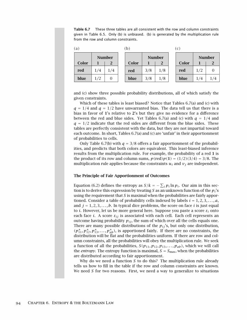
Table 6.7 These three tables are all consistent with the row and column constraintsgiven in Table 6.5. Only (b) is unbiased. (b) is generated by the multiplication rulefrom the row and column constraints.

red

Color

blue

1 2

1/4 1/4

0

Number

(a)

red

Color

blue

Number

(b)

red

Color

blue

Number

(c)

1/2

3/8 1/8

1/83/8

1/2 0

1/41/4

1 2 1 2

and (c) show three possible probability distributions, all of which satisfy thegiven constraints.

Which of these tables is least biased? Notice that Tables 6.7(a) and (c) withq = 1/4 and q = 1/2 have unwarranted bias. The data tell us that there is abias in favor of 1’s relative to 2’s but they give no evidence for a differencebetween the red and blue sides. Yet Tables 6.7(a) and (c) with q = 1/4 andq = 1/2 indicate that the red sides are different from the blue sides. Thesetables are perfectly consistent with the data, but they are not impartial towardeach outcome. In short, Tables 6.7(a) and (c) are ‘unfair’ in their apportionmentof probabilities to cells.

Only Table 6.7(b) with q = 3/8 offers a fair apportionment of the probabil-ities, and predicts that both colors are equivalent. This least-biased inferenceresults from the multiplication rule. For example, the probability of a red 1 isthe product of its row and column sums, p(red)p(1) = (1/2)(3/4) = 3/8. Themultiplication rule applies because the constraints ui and vj are independent.

The Principle of Fair Apportionment of Outcomes

Equation (6.2) defines the entropy as S/k = −∑i pi lnpi. Our aim in this sec-tion is to derive this expression by treating S as an unknown function of thepi’susing the requirement that S is maximal when the probabilities are fairly appor-tioned. Consider a table of probability cells indexed by labels i = 1,2,3, . . . , a,and j = 1,2,3, . . . , b. In typical dice problems, the score on face i is just equalto i. However, let us be more general here. Suppose you paste a score εi ontoeach face i. A score εij is associated with each cell. Each cell represents anoutcome having probability pij , the sum of which over all the cells equals one.There are many possible distributions of the pij ’s, but only one distribution,(p∗11, p

∗12, p

∗13, . . . , p

∗ab), is apportioned fairly. If there are no constraints, the

distribution will be flat and the probabilities uniform. If there are row and col-umn constraints, all the probabilities will obey the multiplication rule. We seeka function of all the probabilities, S(p11, p12, p13, . . . , pab), which we will callthe entropy. The entropy function is maximal, S = Smax, when the probabilitiesare distributed according to fair apportionment.

Why do we need a function S to do this? The multiplication rule alreadytells us how to fill in the table if the row and column constraints are known.We need S for two reasons. First, we need a way to generalize to situations


p3ε3

p1 pnp5p2ε1 εnε5

p4ε4ε2

...

... Row a

Row bpn+1 pm...pn+3pn+2εn+1 εm...εn+3

pn+5εn+5

pn+4εn+4εn+2

Figure 6.5 Two rows a and b in a grid of cells used to illustrate the notation forproving that entropy is extensive. Each row is subject to a constraint on the sum ofprobabilities and a constraint on the sum of the scores.

in which we have only a single constraint, or any set of constraints on onlya part of the system. Second, we seek a measure of the driving force towardredistributing the probabilities when the constraints are changed.

The Principle of Fair Apportionment is all we need to specify the precisemathematical form that the entropy function must have. We will show this intwo steps. First, we will show that the entropy must be extensive. That is, thefunction S that applies to the whole system must be a sum over individual cellfunctions s:

S(p11, p12, p13, . . . , pab)

= s(p11)+ s(p12)+ s(p13)+ · · · + s(pab). (6.26)

Second, we will show that the only function that is extensive and at its maxi-mum satisfies the multiplication rule is the function −∑t

i=1 pi lnpi.

The Entropy Is Extensive

Focus on two collections of cells a and b chosen from within the full grid. Tokeep it simple, we can eliminate the index j if a is a row of cells with proba-bilities that we label (p1, p2, . . . , pn), and b is a different row with probabilitiesthat we label (pn+1, pn+2, . . . , pm) (see Figure 6.5). Our aim is to determinehow the entropy function for the combined system a plus b is related to theentropy functions for the individual rows.

The entropy S is a function that we aim to maximize subject to two condi-tions. Two constraints, g and h, apply to row a: one is the normalization onthe sum of probabilities, and the other is a constraint on the average score,

g(p1, p2, . . . , pn) =n∑i=1

pi = ua,

h(p1, p2, . . . , pn) =n∑i=1

εipi = 〈ε〉a. (6.27)


To find the maximum of a function subject to constraints, use the method ofLagrange multipliers. Multiply (∂g/∂pi) = 1 and (∂h/∂pi) = εi by the corre-sponding Lagrange multipliers αa and λa to get the extremum

∂S(p1, p2, . . . , pn)∂pi

= αa + λaεi. (6.28)

When this equation is satisfied, S is maximal subject to the two constraints.Express the entropy for row a as Sa = S(p1, p2, . . . , pn). To find the totaldifferential for the variation of Sa resulting from any change in the p’s, sumEquation (6.28) over all dpi’s:

dSa =n∑i=1

(∂Sa∂pi

)dpi =

n∑i=1

(αa + λaεi)dpi. (6.29)

Equation (6.29) does not require any assumption about the form of Sa = S(p1,p2, . . . , pn). It is just the definition of the total differential. Similarly, row bin a different part of the grid will be subject to constraints unrelated to theconstraints on row a,

αbm∑

i=n+1

dpi = 0 and λbm∑

i=n+1

εidpi = 0,

with Lagrange multipliers αb and λb. For row b, index i now runs from n+ 1to m, rather than from 1 to n, and we will use the corresponding shorthandnotation Sb = S(pn+1, pn+2, . . . , pm). The total differential for Sb is

dSb =m∑

i=n+1

(∂Sb∂pi

)dpi =

m∑i=n+1

(αb + λbεi)dpi. (6.30)

Finally, use the function Stotal = S(p1, p2, . . . , pn,pn+1, . . . , pm) to apportionprobabilities over both rows a and b at the same time, given exactly the sametwo constraints on row a and the same two constraints on row b as above. Thetotal differential for Stotal is

dStotal =m∑i=1

(∂Stotal

∂pi

)dpi

=n∑i=1

(αa + λaεi)+m∑

i=n+1

(αb + λbεi) = dSa + dSb, (6.31)

where the last equality comes from substitution of Equations (6.29) and (6.30).This says that if the entropy is to be a function having a maximum, subjectto constraints on blocks of probability cells, then it must be extensive. Theentropy of a system is a sum of subsystem entropies. The underlying premiseis that the score quantities, 〈ε〉a and 〈ε〉b, are extensive.

The way in which we divided the grid into rows a and b was completelyarbitrary. We could have parsed the grid in many different ways, down to anindividual cell at a time. Following this reasoning to its logical conclusion,and integrating the differentials, leads to Equation (6.26), which shows that theentropy of the whole grid is the sum of entropies of the individual cells.


The Form of the Entropy Function

To obtain the form of the entropy function, we use a table of probabilitieswith rows labeled by the index i and columns by the index j. Each row i isconstrained to have an average score,

b∑j=1

εijpij = 〈εi〉 �⇒ λib∑j=1

εijdpij = 0, (6.32)

where λi is the Lagrange multiplier that enforces the score constraint for rowi. Similarly, for column j,

βja∑i=1

εijdpij = 0,

where βj is the Lagrange multiplier that enforces the score constraint for col-umn j. Finally,

α∑ijdpij = 0

enforces the constraint that the probabilities must sum to one over the wholegrid of cells. We use the extensivity property, Equation (6.26), to find the ex-pression for maximizing the entropy subject to these three constraints,

a∑i=1

b∑j=1

[(∂s(pij)∂pij

)− λiεij − βjεij −α

]dpij = 0. (6.33)

To solve Equation (6.33), each term in brackets must equal zero for eachcell ij according to the Lagrange method (see Equation (5.35)).

Our aim is to deduce the functional form for s(pij) by determining howEquation (6.33) responds to changes in the row constraint ui and column con-straint vj . To look at this dependence, let’s simplify the notation. Focus onthe term in the brackets, for one cell ij, and drop the subscripts ij for now.Changing the row or column sum u or v changes p, so express the dependenceas p(u,v).

Define the derivative (∂sij/∂pij) = rij , and express it as r[p(u,v)]. Thequantities εij differ for different cells in the grid, but they are fixed quantitiesand do not depend on u or v . Because the probabilities must sum to oneover the whole grid no matter what changes are made in u and v , α is alsoindependent of u and v . The value of the Lagrange multipliers λ(u) for row iand β(v) for column j will depend on the value of the constraints u and v (seeExample 6.5). Collecting together these functional dependences, the bracketedterm in Equation (6.33) can be expressed as

r[p(u,v)] = λ(u)ε + β(v)ε +α. (6.34)

Now impose the multiplication rule, p = uv . Let’s see how r depends on uand v . This will lead us to specific requirements for the form of the entropyfunction. Take the derivative of Equation (6.34) with respect to v to get


(∂r∂v

)=(∂r∂p

)(∂p∂v

)=(∂r∂p

)pv= εβ′(v). (6.35)

where β′ = dβ/dv and (∂p/∂v) = u = p/v . Now take the derivative of Equa-tion (6.34) with respect to u instead of v to get(

∂r∂p

)pu= ελ′(u), (6.36)

where λ′ = dλ/du. Rearranging and combining Equations (6.35) and (6.36)gives(

∂r∂p

)= uλ′(u)ε

p= vβ′(v)ε

p. (6.37)

Notice that the quantity uλ′(u)ε can only depend on (east–west) propertiesof the row i, particularly its sum u. Likewise, the quantity vβ′(v)ε can onlydepend on (north–south) properties of the column j, particularly its sum v .The only way that these two quantities can be equal in Equation (6.37) for anyarbitrary values of u and v is if uλ′(u)ε = vβ′(v)ε = constant. Call thisconstant −k, and you have(

∂r∂p

)= −kp. (6.38)

Integrate Equation (6.38) to get

r(p) = −k lnp + c1,

where c1 is the constant of integration. To get s(p), integrate again:

s(p) =∫r(p)dp =

∫(−k lnp + c1)dp

= −k(p lnp − p)+ c1p + c2, (6.39)

where c2 is another constant of integration. Summing over all cells ij gives thetotal entropy:

S =a∑i=1

b∑j=1

s(pij) = −k∑ijpij lnpij + c3

∑ijpij + c2, (6.40)

where c3 = k + c1. Since∑ij pij = 1, the second term on the right side of

Equation (6.40) sums to a constant, and Equation (6.40) becomes

S = −k∑ijpij lnpij + constant. (6.41)

If you define the entropy of a perfectly ordered state (one pij equals one, allothers equal zero) to be zero, the constant in Equation (6.41) equals zero. If youchoose the convention that the extremum of S should be a maximum ratherthan a minimum, k is a positive constant. If there is only a single cell index i,you have S/k = −∑i pi lnpi.

Equation (6.41) is a most remarkable result. It says that you can uniquely de-fine a function, the entropy, that at its maximum will assign probabilities to the


x1

x2

x1 + x2 = u1

x1 + x2 = u2

f (x1, x2) = 18 − (2x1 + 2x2)2 2 Figure 6.6 The optimum of f(x1, x2)

changes if a row sum g = x1 + x2 = uchanges from a value u1 to u2.

cells in accordance with the Fair Apportionment Principle: (1) when there are noconstraints, all probabilities will be equal, and (2) when there are independentconstraints, the probabilities will satisfy the multiplication rule. Because S isthe only function that succeeds at this task when it is maximal, S must alsobe the only function that gives the deviations from the Fair ApportionmentPrinciple when it is not maximal.

EXAMPLE 6.5 Illustrating the dependence λ(u). A Lagrange multiplier candepend on the value of a row (or column) constraint. Consider a functionf(x1, x2) = 18− (2x2

1 +2x22) subject to the constraint g(x1, x2) = x1+x2 = u

(see Figure 6.6). The extremum is found where(∂f∂x1

)= −4x1 = λ, and

(∂f∂x2

)= −4x2 = λ �⇒ x1 = x2 = −λ

4. (6.42)

Substitute Equation (6.42) into g = x1 + x2 = u to find λ(u) = −2u.

Philosophical Foundations

For more than a century, entropy has been a controversial concept. One issueis whether entropy is a tool for making predictions based on the knowledgeof an observer [1], or whether it is independent of an observer [3]. Both in-terpretations are useful under different circumstances. For dice and coin flipproblems, constraints such as an average score define the limited knowledgethat you have. You want to impart a minimum amount of bias in predicting theprobability distribution that is consistent with that knowledge. Your predictionshould be based on assuming you are maximally ignorant with respect to allelse [1, 4]. Maximizing the function −∑i pi lnpi serves the role of making thisprediction. Similar prediction problems arise in eliminating noise from spec-troscopic signals or in reconstructing satellite photos. In these cases, the Prin-ciple we call Fair Apportionment describes how to reason and draw inferences

Philosophical Foundations 99

and make the least-biased predictions of probabilities in face of incompleteknowledge.

However, for other problems, notably those of statistical mechanics, en-tropy describes a force of nature. In those cases, constraints such as averagesover a row of probabilities are not only numbers that are known to an observer,they are also physical constraints that are imposed upon a physical system fromoutside (see Chapter 10). In this case, the Principle of Fair Apportionment is adescription of nature’s symmetries. When there is an underlying symmetry ina problem (such as t outcomes that are equivalent), then Fair Apportionmentsays that external constraints are shared equally between all the possible statesthat the system can occupy (grid cells, in our earlier examples). In this case,entropy is more than a description about an observer. It describes a tendencyof nature that is independent of an observer.

A second controversy involves the interpretation of probabilities. The twoperspectives are the frequency interpretation and the ‘inference’ interpreta-tion [1]. According to the frequency interpretation, a probability pA = nA/Ndescribes some event that can be repeated N times. However, the inference in-terpretation is broader. It says that probabilities are fractional quantities thatdescribe a state of knowledge. In the inference view, the rules of probability aresimply rules for making consistent inferences from limited information. Theprobability that it might rain tomorrow, or the probability that Elvis Presleywas born on January 8, can be perfectly well defined, even though these eventscannot be repeatedN times. In the inference view, probabilities can take on dif-ferent values depending on your state of knowledge. If you do not know whenElvis was born, you would say the probability is 1/365 that January 8 was hisbirthday. That is a statement about your lack of knowledge. However, if youhappen to know that was his birthday, the probability is one. According to thesubjective interpretation, the rules of probability theory in Chapter 1 are lawsfor drawing consistent inferences from incomplete information, irrespective ofwhether or not the events are countable.

Historically, statistical mechanics has been framed in terms of the frequencyinterpretation. JW Gibbs (1839–1903), American mathematical physicist and afounder of chemical thermodynamics and statistical mechanics, framed statis-tical mechanics as a counting problem. He envisioned an imaginary collectionof all possible outcomes, called an ensemble, which was countable and couldbe taken to the limit of a large number of imaginary repetitions. To be specific,for die rolls, if you want to know the probability of each of the six outcomeson a roll, the ensemble approach would be to imagine that you had rolled thedie N times. You would then compute the number of sequences that you ex-pect to observe. This number will depend on N . On the other hand, if theoutcomes can instead be described in terms of probabilities, the quantity Nnever appears. For example, the grid of cells described in Table 6.2 describesprobabilities that bear no trace of the information that N = 1000 die rolls wereused to obtain Table 6.1.

These issues are largely philosophical fine points that have had little impli-cation for the practice of statistical mechanics. We will sometimes prefer thecounting strategy, and the use of S/k = lnW , but S/k = −∑i pi lnpi will bemore convenient in other cases.


Summary

The entropy S(p11, . . . , pij, . . . , pab) is a function of a set of probabilities. Thedistribution of pij ’s that cause S to be maximal is the distribution that mostfairly apportions the constrained scores between the individual outcomes. Thatis, the probability distribution is flat if there are no constraints, and follows themultiplication rule of probability theory if there are independent constraints. Ifthere is a constraint, such as the average score on die rolls, and if it is not equalto the value expected from a uniform distribution, then maximum entropy pre-dicts an exponential distribution of the probabilities. In Chapter 10, this expo-nential function will define the Boltzmann distribution law. With this law youcan predict thermodynamic and physical properties of atoms and molecules,and their averages and fluctuations. However, first we need the machinery ofthermodynamics, the subject of the next three chapters.

Summary 101

Problems

1. Calculating the entropy of dipoles in a field. Youhave a solution of dipolar molecules with a positive chargeat the head and a negative charge at the tail. When thereis no electric field applied to the solution, the dipolespoint north (n), east (e), west (w), or south (s) with equalprobabilities. The probability distribution is shown in Fig-ure 6.7(a). However when you apply a field to the solution,you now observe a different distribution, with more headspointing north, as shown in Figure 6.7(b).

(a) What is the polarity of the applied field? (In whichdirection does the field have its most positive pole?)

(b) Calculate the entropy of the system in the absenceof the field.

(c) Calculate the entropy of the system in the appliedfield.

(d) Does the system become more ordered or disor-dered when the field is applied?

n e w s n e w s

(a) Electric Field Absent (b) Electric Field Present

PP

14

14

14

14

14

14

116

716

Figure 6.7

2. Comparing the entropy of peaked and flat distri-butions. Compute the entropies for the spatial concen-tration shown in Figures 6.8(a) and (b).

P

(a) Peaked Distribution (b) Flat Distribution

0 0 0 0

1

P

x x

15

15

15

15

15

Figure 6.8

3. Comparing the entropy of two peaked distributions.Which of the two distributions shown in Figure 6.9 has thegreater entropy?

P

1 2 3 4Outcome

1 2 3 4Outcome

(a) Outcome 1 is Favored (b) Outcome 2 is Favored

P

16

12

16

16

12

16

16

16

Figure 6.9

4. Calculating the entropy of mixing. Consider a latticewith N sites and n green particles. Consider another lat-tice, adjacent to the first, withM sites andm red particles.Assume that the green and red particles cannot switch lat-tices. This is state A.

(a) What is the total number of configurations WA ofthe system in state A?

(b) Now assume that all N +M sites are available to allthe green and red particles. The particles remaindistinguishable by their color. This is state B. Nowwhat is the total number of configurationsWB of thesystem?

Now take N = M and n = m for the following two prob-lems.

(c) Using Stirling’s approximation on page 56, what isthe ratio WA/WB?

(d) Which state, A or B, has the greatest entropy? Cal-culate the entropy difference given by

∆S = SA − SB = k ln(WAWB

).

5. Proof of maximum entropy for two outcomes. Ex-ample 6.4 (page 88) is simple enough that you can provethe answer is correct even without using the maximumentropy principle. Show this.

6. Proving the multiplication rule maximizes the en-tropy. Show that if the entropy is defined by Equa-tion (6.2), S/k = −∑i pi lnpi, and if the 2× 2 grids of Ta-bles 6.4 through 6.7 have row sumsu1 andu2, and columnsums v1 and v2, then the function pij(ui, vj) that maxi-mizes the entropy is the multiplication rule pij = uivj .

7. Other definitions of entropy do not satisfy the mul-tiplication rule. In contrast to problem 6, show that ifthe entropy were defined by a least-squares criterion, asS/k =∑t

i=1 p2i , the multiplication rule would not be satis-

fied when S is maximal.


8. Other definitions of entropy can predict the uniformdistribution when there are no constraints. As inproblem 7, assume that the definition of entropy wasS/k = ∑t

i=1 p2i . Show that when there are no row or col-

umn constraints on the 2× 2 grids of Tables 6.4 through6.7, the definition will satisfactorily predict that the uni-form distribution is an extremum of the entropy.

9. The maximum entropy distribution is Gaussian whenthe second moment is given. Prove that the probabil-ity distribution pi that maximizes the entropy for die rollssubject to a constant value of the second moment 〈i2〉 isa Gaussian function. Use εi = i.

10. Maximum entropy for a three-sided die. You havea three-sided die, with numbers 1, 2 and 3 on the sides.For a series of N dice rolls, you observe an average score〈ε〉 per roll using the maximum entropy principle.

(a) Write expressions that show how to compute the rel-ative probabilities of occurrence of the three sides,n∗1 /N , n∗2 /N , and n∗3 /N , if α is given.

(b) Compute n∗1 /N , n∗2 /N , and n∗3 /N if α = 2.

(c) Compute n∗1 /N , n∗2 /N , and n∗3 /N , if α = 1.5.

(d) Compute n∗1 /N , n∗2 /N , and n∗3 /N if α = 2.5.

11. Maximum entropy in Las Vegas. You play a slotmachine in Las Vegas. For every $1 coin you insert, thereare three outcomes: (1) you lose $1, (2) you win $1, so yourprofit is $0, (3) you win $5, so your profit is $4. Supposeyou find that your average expected profit over many tri-als is $0 (what an optimist!). Find the maximum entropydistribution for the probabilities p1, p2, and p3 of observ-ing each of these three outcomes.

12. Flat distribution, high entropy. For four coinflips, for each distribution of probabilities, (pH,pT ) =(0,1), (1/4,3/4), (1/2,1/2), (3/4,1/4), (1,0), computeW , and show that the flattest distribution has the highestmultiplicity.

References

[1] ET Jaynes. The Maximum Entropy Formalism, RDLevine and M Tribus eds., MIT Press, Cambridge, 1979,page 15.

[2] RT Cox. Am J Phys 14, 1 (1946).

[3] KG Denbigh and JS Denbigh. Entropy in Relation toIncomplete Knowledge. Cambridge University Press,Cambridge, 1985.

[4] ET Jaynes. Phys Rev 106, 620 (1957).

Suggested Reading

ET Jaynes, Phys Rev 106, 620 (1957). This is the clas-sic article that introduces the maximum entropy ap-proach to statistical thermodynamics. It is well-written and includes a scholarly historical introduc-tion.

JN Kapur and HK Kesavan, Entropy Optimization Princi-ples with Applications, Academic Press, Boston, 1992.Excellent overview of maximum entropy applied tomany fields of science.

RD Levine and M Tribus, The Maximum Entropy Formal-ism, MIT Press, 1979. This is an advanced edited vol-ume that discusses applications and other aspects ofmaximum entropy, including an extensive review byJaynes.

The following three articles show how the maximum en-tropy principle follows from the multiplication rule. Abrief overview is given in J Skilling, Nature, 309, 748(1984).

AK Livesay and J Skilling, Acta Crystallographica, A41,113–122 (1985).

JE Shore and RW Johnson, IEEE Trans Inform Theory 26,26 (1980).

Y Tikochinski, NZ Tishby, RD Levine, Phys Rev Lett 52,1357 (1984).

Suggested Reading 103

6entropy & the boltzmann law - brandeis university2004-9-29 · 6entropy & the boltzmann...

Documents