A central limit theorem for the sample

autocorrelations of a Levy driven continuous time

moving average process

Serge Cohen∗ Alexander Lindner†

Abstract

In this article we consider Levy driven continuous time moving average pro-

cesses observed on a lattice, which are stationary time series. We show asymptotic

normality of the sample mean, the sample autocovariances and the sample autocor-

relations. A comparison with the classical setting of discrete moving average time

series shows that in the last case a correction term should be added to the classical

Bartlett formula that yields the asymptotic variance. An application to the asymp-

totic normality of the estimator of the Hurst exponent of fractional Levy processes

is also deduced from these results.

Keywords: Bartlett’s formula, continuous time moving average process, estimation

of the Hurst index, fractional Levy process, Levy process, limit theorem, sample

autocorrelation, sample autocovariance, sample mean.

1 Introduction

Statistical models are often written in a continuous time setting for theoretical

reasons (e.g. diffusions). But if one wants to estimate the parameters of these models,

one usually assumes only the observation of a discrete sample. At this point a very

general question, the answer of which depends on the model chosen, is to know if the

estimation should not have been performed with an underlying discrete model in

the beginning. In this article we will consider this for moving average processes and

∗Institut de Mathematiques de Toulouse, Universite Paul Sabatier, Universite de Toulouse, 118 route

de Narbonne F-31062 Toulouse Cedex 9. E-mail: Serge.Cohen@math.univ-toulouse.fr†Institut fur Mathematische Stochastik, Technische Universitat Braunschweig, Pockelsstraße 14, D-

38106 Braunschweig, Germany. E-mail: a.lindner@tu-bs.de

1

we refer to the classical moving average time series models as a discrete counterpart

of this continuous model.

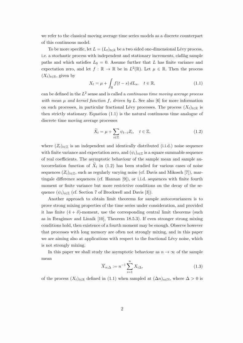
To be more specific, let L = (Lt)t∈R be a two sided one-dimensional Levy process,

i.e. a stochastic process with independent and stationary increments, cadlag sample

paths and which satisfies L0 = 0. Assume further that L has finite variance and

expectation zero, and let f : R → R be in L2(R). Let µ ∈ R. Then the process

(Xt)t∈R, given by

Xt = µ+

∫Rf(t− s) dLs, t ∈ R, (1.1)

can be defined in the L2 sense and is called a continuous time moving average process

with mean µ and kernel function f , driven by L. See also [6] for more information

on such processes, in particular fractional Levy processes. The process (Xt)t∈R is

then strictly stationary. Equation (1.1) is the natural continuous time analogue of

discrete time moving average processes

Xt = µ+∑i∈Z

ψt−iZi, t ∈ Z, (1.2)

where (Zt)t∈Z is an independent and identically distributed (i.i.d.) noise sequence

with finite variance and expectation zero, and (ψi)i∈Z is a square summable sequence

of real coefficients. The asymptotic behaviour of the sample mean and sample au-

tocorrelation function of Xt in (1.2) has been studied for various cases of noise

sequences (Zi)i∈Z, such as regularly varying noise (cf. Davis and Mikosch [7]), mar-

tingale difference sequences (cf. Hannan [9]), or i.i.d. sequences with finite fourth

moment or finite variance but more restrictive conditions on the decay of the se-

quence (ψi)i∈Z (cf. Section 7 of Brockwell and Davis [3]).

Another approach to obtain limit theorems for sample autocovariances is to

prove strong mixing properties of the time series under consideration, and provided

it has finite (4 + δ)-moment, use the corresponding central limit theorems (such

as in Ibragimov and Linnik [10], Theorem 18.5.3). If even stronger strong mixing

conditions hold, then existence of a fourth moment may be enough. Observe however

that processes with long memory are often not strongly mixing, and in this paper

we are aiming also at applications with respect to the fractional Levy noise, which

is not strongly mixing.

In this paper we shall study the asymptotic behaviour as n→ ∞ of the sample

mean

Xn;∆ := n−1n∑

i=1

Xi∆, (1.3)

of the process (Xt)t∈R defined in (1.1) when sampled at (∆n)n∈N, where ∆ > 0 is

2

fixed, and of its sample autocovariance and sample autocorrelation function

γn;∆(∆h) := n−1n−h∑i=1

(Xi∆ −Xn;∆)(X(i+h)∆ −Xn;∆), h ∈ {0, . . . , n− 1}, (1.4)

ρn;∆(∆h) := γn;∆(∆h)/γn;∆(0), h ∈ {0, . . . , n− 1}. (1.5)

We write N = {0, 1, 2, . . .}. Under appropriate conditions on f and L, in particular

assuming L to have finite fourth moment for the sample autocorrelation functions, it

will be shown that Xn;∆ and (ρn;∆(∆), . . . , ρn;∆(h∆)) are asymptotically normal for

each h ∈ N as n → ∞. This is similar to the case of discrete time moving average

processes of the form (1.2) with i.i.d. noise, but unlike for those, the asymptotic

variance of the sample autocorrelations of model (1.1) will turn out to be given by

Bartlett’s formula plus an extra term which depends explicitly on the fourth moment

of L, and in general this extra term does not vanish. This also shows that the “naive”

approach of trying to write the sampled process (Xn∆)n∈Z as a discrete time moving

average process as in (1.2) with i.i.d. noise does not work in general, since for such

processes the asymptotic variance would be given by Bartlett’s formula only. If

µ = 0, then further natural estimators of the autocovariance and autocorrelation

are given by

γ∗n;∆(∆h) := n−1n∑

i=1

Xi∆X(i+h)∆, h ∈ {0, . . . , n− 1}, (1.6)

ρ∗n;∆(∆h) := γ∗n;∆(∆h)/γ∗n;∆(0), h ∈ {0, . . . , n− 1}, (1.7)

and the conditions we have to impose to get asymptotic normality of γ∗n;∆ and ρ∗n;∆are less restrictive than those for γn;∆ and ρn;∆.

We will be particularly interested in the case when f decays like a polynomial,

which is e.g. the case for fractional Levy noises. For a given Levy process with

expectation zero and finite variance, and a parameter d ∈ (0, 1/2), the (moving

average) fractional Levy process (M1t;d)t∈R with Hurst parameter H := d + 1/2 is

given by

M1t;d :=

1

Γ(d+ 1)

∫ ∞

−∞

[(t− s)d+ − (−s)d+

]dLs, t ∈ R (1.8)

(cf. Marquardt [11]). A process also called fractional Levy process was introduced

before by Benassi et al. [2], where (x)+ = max(x, 0) is replaced by an absolute value

in (1.8),

M2t;d :=

∫ ∞

−∞

[|t− s|d − |s|d

]dLs, t ∈ R. (1.9)

Although both processes have different distributions, they enjoy similar properties.

For instance the sample paths of both versions are Holder continuous, have the same

pointwise Holder exponent, and they are both locally self-similar (see [2] for the

3

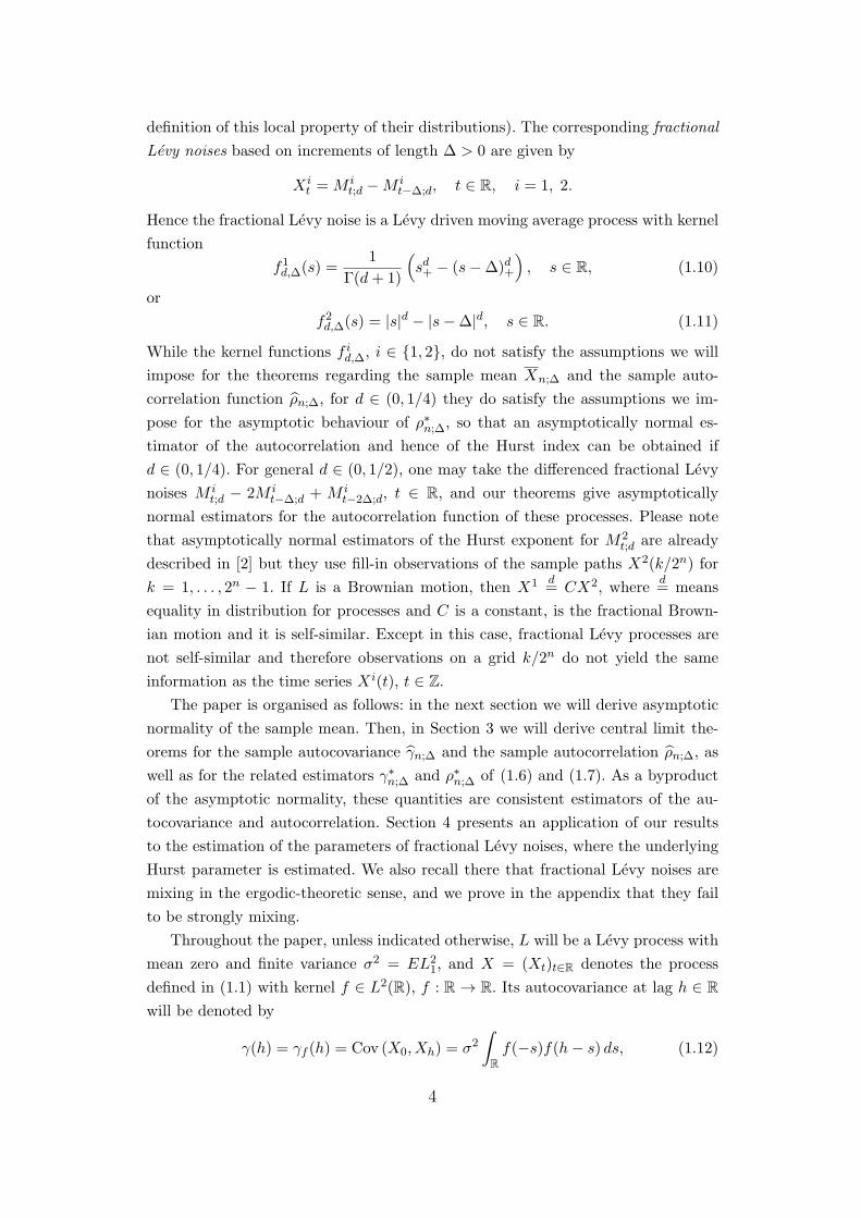
definition of this local property of their distributions). The corresponding fractional

Levy noises based on increments of length ∆ > 0 are given by

Xit =M i

t;d −M it−∆;d, t ∈ R, i = 1, 2.

Hence the fractional Levy noise is a Levy driven moving average process with kernel

function

f1d,∆(s) =1

Γ(d+ 1)

(sd+ − (s−∆)d+

), s ∈ R, (1.10)

or

f2d,∆(s) = |s|d − |s−∆|d, s ∈ R. (1.11)

While the kernel functions f id,∆, i ∈ {1, 2}, do not satisfy the assumptions we will

impose for the theorems regarding the sample mean Xn;∆ and the sample auto-

correlation function ρn;∆, for d ∈ (0, 1/4) they do satisfy the assumptions we im-

pose for the asymptotic behaviour of ρ∗n;∆, so that an asymptotically normal es-

timator of the autocorrelation and hence of the Hurst index can be obtained if

d ∈ (0, 1/4). For general d ∈ (0, 1/2), one may take the differenced fractional Levy

noises M it;d − 2M i

t−∆;d + M it−2∆;d, t ∈ R, and our theorems give asymptotically

normal estimators for the autocorrelation function of these processes. Please note

that asymptotically normal estimators of the Hurst exponent for M2t;d are already

described in [2] but they use fill-in observations of the sample paths X2(k/2n) for

k = 1, . . . , 2n − 1. If L is a Brownian motion, then X1 d= CX2, where

d= means

equality in distribution for processes and C is a constant, is the fractional Brown-

ian motion and it is self-similar. Except in this case, fractional Levy processes are

not self-similar and therefore observations on a grid k/2n do not yield the same

information as the time series Xi(t), t ∈ Z.The paper is organised as follows: in the next section we will derive asymptotic

normality of the sample mean. Then, in Section 3 we will derive central limit the-

orems for the sample autocovariance γn;∆ and the sample autocorrelation ρn;∆, as

well as for the related estimators γ∗n;∆ and ρ∗n;∆ of (1.6) and (1.7). As a byproduct

of the asymptotic normality, these quantities are consistent estimators of the au-

tocovariance and autocorrelation. Section 4 presents an application of our results

to the estimation of the parameters of fractional Levy noises, where the underlying

Hurst parameter is estimated. We also recall there that fractional Levy noises are

mixing in the ergodic-theoretic sense, and we prove in the appendix that they fail

to be strongly mixing.

Throughout the paper, unless indicated otherwise, L will be a Levy process with

mean zero and finite variance σ2 = EL21, and X = (Xt)t∈R denotes the process

defined in (1.1) with kernel f ∈ L2(R), f : R → R. Its autocovariance at lag h ∈ Rwill be denoted by

γ(h) = γf (h) = Cov (X0, Xh) = σ2∫Rf(−s)f(h− s) ds, (1.12)

4

where the last equation follows from the Ito isometry.

Let us set some notations used in the sequel.

If v is vector and A is a matrix, their transposes are denoted by v′ and A′

respectively.

Convergence in distribution is denoted byd→.

The function 1A for a set A is one for x ∈ A, and zero elsewhere.

The autocorrelation of X at lag h will be denoted by ρ(h) = ρf (h) = γ(h)/γ(0).

2 Asymptotic normality of the sample mean

The sample mean Xn;∆ of the moving average process X of (1.1) behaves like the

sample mean of a discrete time moving average process with i.i.d. noise, in the sense

that it is asymptotically normal with variance σ2∑∞

k=−∞ γ(k∆), provided the latter

is absolutely summable.

Theorem 2.1. Let L have zero mean and variance σ2, let µ ∈ R and ∆ > 0.

Suppose thatF∆ : [0,∆] → [0,∞], u 7→ F∆(u) =

∞∑j=−∞

|f(u+ j∆)|

∈ L2([0,∆]). (2.1)

Then∑∞

j=−∞ |γ(∆j)| <∞,

∞∑j=−∞

γ(∆j) = σ2∫ ∆

0

∞∑j=−∞

f(u+ j∆)

2

du, (2.2)

and the sample mean of X∆, . . . , Xn∆ is asymptotically normal as n → ∞. More

precisely

√n (Xn;∆ − µ)

d→ N

0, σ2∫ ∆

0

∞∑j=−∞

f(u+∆j)

2

du

as n→ ∞.

Remark 2.2. Throughout the paper the assumption that L has zero mean can be

dropped very often. For instance, if f ∈ L1(R)∩L2(R), then the assumption of zero

mean of L presents no restriction, for in that case L′t := Lt− tE(L1), t ∈ R, defines

another Levy process with mean zero and the same variance, and it holds

Xt = µ+E(L1)

∫Rf(s) ds+

∫Rf(t− s) dL′

s, t ∈ Z, (2.3)

which has mean µ+ E(L1)∫R f(s) ds.

5

Proof. For simplicity in notation, assume that ∆ = 1, and write F = F1. Continue

F periodically on R by setting

F (u) =∞∑

j=−∞|f(u+ j)|, u ∈ R.

Since

|γf (h)| ≤ σ2∫ ∞

−∞|f(−s)| |f(h− s)| ds

by (1.12), we have

1

σ2

∞∑h=−∞

|γf (h)| ≤∫ ∞

−∞|f(−s)|

∞∑h=−∞

|f(h− s)| ds

=

∫ ∞

−∞|f(s)|F (s) ds

=∞∑

j=−∞

∫ 1

0|f(s+ j)|F (s) ds

=

∫ 1

0F (s)F (s) ds <∞. (2.4)

The same calculation without the modulus gives (2.2).

The proof for asymptotic normality is now much in the same spirit as for discrete

time moving average processes, by reducing the problem to m-dependent sequences

first and then applying an appropriate variant of Slutsky’s theorem. By subtracting

the mean we may assume without loss of generality that µ = 0. For m ∈ N, letfm := f 1(−m,m), and denote

X(m)t :=

∫Rfm(s) dLs =

∫ t+m

t−mf(t− s) dLs, t ∈ Z.

Observe that (X(m)t )t∈Z is a (2m−1)-dependent sequence, i.e. (X

(m)j )j≤t and (X

(m)j )j≥t+2m

are independent for each t ∈ Z. From the central limit theorem for strictly station-

ary (2m − 1)-dependent sequences (cf. Theorem 6.4.2 in Brockwell and Davis [3])

we then obtain that

√nX

(m)n;1 = n−1/2

n∑t=1

X(m)t

d→ Y (m), n→ ∞, (2.5)

where Y (m) is a random variable such that

Y (m) d= N(0, vm)

with vm =∑2m

j=−2m γfm(j). Since limm→∞ γfm(j) = γf (j) for each j ∈ Z by (1.12),

since

|γf1(−m,m)(j)|≤σ2

∫ ∞

−∞|f(−s)| |f(j − s)| ds,

6

and∑∞

j=−∞∫∞−∞ |f(−s)| |f(j − s)| < ∞ by (2.4), it follows from Lebesgue’s domi-

nated convergence theorem that limm→∞ vm =∑∞

j=−∞ γf (j). Hence by (2.2),

Y (m) d→ Y, m→ ∞, where Yd= N

0, σ2∫ 1

0

∞∑j=−∞

f(u+ j)

2

du

. (2.6)

A similar argument gives limm→∞∑∞

j=−∞ γf−fm(j) = 0, so that

limm→∞

limn→∞

Var(n1/2(Xn;1 −X

(m)n;1 )

)= lim

m→∞limn→∞

nVar

(n−1

n∑t=1

∫ ∞

−∞(f(t− s)− fm(t− s)) dLs

)

= limm→∞

∞∑j=−∞

γf−fm(j) = 0,

where we used Theorem 7.1.1 in Brockwell and Davis [3] for the second equality.

An application of Chebychef’s inequality then shows that

limm→∞

lim supn→∞

P (n1/2|Xn;1 −X(m)n;1 | > ε) = 0

for every ε > 0. Together with (2.5) and (2.6) this implies the claim by a variant of

Slutsky’s theorem (cf. [3], Proposition 6.3.9).

Remark 2.3. Let us start with an easy remark on a necessary condition on the

kernel f to apply the previous theorem. Obviously F∆ ∈ L1([0,∆]) is equivalent to

f ∈ L1(R). Hence F∆ ∈ L2([0,∆]) ⇒ f ∈ L1(R).

Remark 2.4. Unlike for the discrete time moving average process of (1.2), where

absolute summability of the autocovariance function is guaranteed by absolute summa-

bility of the coefficient sequence, for the continuous time series model (1.1) it is not

enough to assume that the kernel satisfies f ∈ L1(R) ∩ L2(R). An example is given

by taking ∆ = 1 and

f(u) :=

0, u ≤ 0,

1, u ∈ [0, 1),

1·3···(2j−1)2jj!

(u− j)j , u ∈ [j, j + 1), j ∈ N.

For then the function F1 is given by

F1(u) =∑j∈Z

f(u+ j) = (1− u)−1/2, u ∈ [0, 1),

so that F1 ∈ L1([0, 1]) \ L2([0, 1]). But F1 ∈ L1([0, 1]) is equivalent to f ∈ L1(R),and since |f(u)| ≤ 1 for all u ∈ R, this implies also f ∈ L2(R). Observe further that

for non-negative f , condition (2.1) is indeed necessary and sufficient for absolute

summability of the autocovariance function.

7

3 Asymptotic normality of the sample auto-

covariance

As usual, we consider the stationary process

Xt =

∫ ∞

−∞f(t− s) dLs, t ∈ R. (3.1)

We recall that

γ∗n;∆(h∆) = n−1n∑

t=1

Xt∆X(t+h)∆, h ∈ N

and first we establish an asymptotic result for Cov (γ∗n;∆(p∆), γ∗n;∆(q∆)).

Proposition 3.1. Let L be a (non-zero) Levy process, with expectation zero, and

finite fourth moment, and denote σ2 := EL21 and η := σ−4EL4

1. Let ∆ > 0, and

suppose further that f ∈ L2(R) ∩ L4(R) and that([0,∆] → R, u 7→

∞∑k=−∞

f(u+ k∆)2

)∈ L2([0,∆]). (3.2)

For q ∈ Z define the function

gq;∆ : [0,∆] → R, u 7→∞∑

k=−∞f(u+ k∆)f(u+ (k + q)∆),

which belongs to L2([0,∆]), by the previous assumption. If further

∞∑h=−∞

|γ(h∆)|2 <∞, (3.3)

then we have for each p, q ∈ N

limn→∞

nCov (γ∗n;∆(p∆), γ∗n;∆(q∆)) = (η − 3)σ4∫ ∆

0gp;∆(u)gq;∆(u) du+

∞∑k=−∞

[γ(k∆)γ((k − p+ q)∆) + γ((k + q)∆)γ((k − p)∆)

]. (3.4)

Proof. For simplicity in notation we assume that ∆ = 1. The general case can be

proved analogously or reduced to the case ∆ = 1 by a simple time change. We shall

first show that for t, p, h, q ∈ Z

E(XtXt+pXt+h+qXt+h+p+q)

= (η − 3)σ4∫ ∞

−∞f(u)f(u+ p)f(u+ h+ p)f(u+ h+ p+ q) du

+γ(p)γ(q) + γ(h+ p)γ(h+ q) + γ(h+ p+ q)γ(h). (3.5)

8

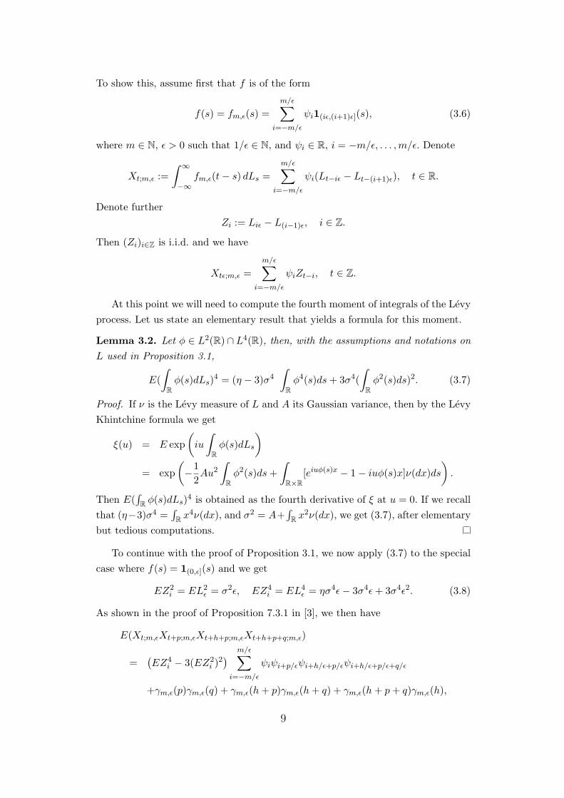
To show this, assume first that f is of the form

f(s) = fm,ϵ(s) =

m/ϵ∑i=−m/ϵ

ψi1(iϵ,(i+1)ϵ](s), (3.6)

where m ∈ N, ϵ > 0 such that 1/ϵ ∈ N, and ψi ∈ R, i = −m/ϵ, . . . ,m/ϵ. Denote

Xt;m,ϵ :=

∫ ∞

−∞fm,ϵ(t− s) dLs =

m/ϵ∑i=−m/ϵ

ψi(Lt−iϵ − Lt−(i+1)ϵ), t ∈ R.

Denote further

Zi := Liϵ − L(i−1)ϵ, i ∈ Z.

Then (Zi)i∈Z is i.i.d. and we have

Xtϵ;m,ϵ =

m/ϵ∑i=−m/ϵ

ψiZt−i, t ∈ Z.

At this point we will need to compute the fourth moment of integrals of the Levy

process. Let us state an elementary result that yields a formula for this moment.

Lemma 3.2. Let ϕ ∈ L2(R) ∩ L4(R), then, with the assumptions and notations on

L used in Proposition 3.1,

E(

∫Rϕ(s)dLs)

4 = (η − 3)σ4∫Rϕ4(s)ds+ 3σ4(

∫Rϕ2(s)ds)2. (3.7)

Proof. If ν is the Levy measure of L and A its Gaussian variance, then by the Levy

Khintchine formula we get

ξ(u) = E exp

(iu

∫Rϕ(s)dLs

)= exp

(−1

2Au2

∫Rϕ2(s)ds+

∫R×R

[eiuϕ(s)x − 1− iuϕ(s)x]ν(dx)ds

).

Then E(∫R ϕ(s)dLs)

4 is obtained as the fourth derivative of ξ at u = 0. If we recall

that (η−3)σ4 =∫R x

4ν(dx), and σ2 = A+∫R x

2ν(dx), we get (3.7), after elementary

but tedious computations.

To continue with the proof of Proposition 3.1, we now apply (3.7) to the special

case where f(s) = 1(0,ϵ](s) and we get

EZ2i = EL2

ϵ = σ2ϵ, EZ4i = EL4

ϵ = ησ4ϵ− 3σ4ϵ+ 3σ4ϵ2. (3.8)

As shown in the proof of Proposition 7.3.1 in [3], we then have

E(Xt;m,ϵXt+p;m,ϵXt+h+p;m,ϵXt+h+p+q;m,ϵ)

=(EZ4

i − 3(EZ2i )

2) m/ϵ∑i=−m/ϵ

ψiψi+p/ϵψi+h/ϵ+p/ϵψi+h/ϵ+p/ϵ+q/ϵ

+γm,ϵ(p)γm,ϵ(q) + γm,ϵ(h+ p)γm,ϵ(h+ q) + γm,ϵ(h+ p+ q)γm,ϵ(h),

9

where γm,ϵ(u) = E(X0;m,ϵXu;m,ϵ), u ∈ R. By (3.8),

EZ4i − 3(EZ2

i )2 = (η − 3)σ4ϵ,

and

ϵ

m/ϵ∑i=−m/ϵ

ψiψi+p/ϵψi+h/ϵ+p/ϵψi+h/ϵ+p/ϵ+q/ϵ

=

∫ ∞

−∞f(u)f(u+ p)f(u+ h+ p)f(u+ h+ p+ q) du,

so that (3.5) follows for f of the form f = fm,ϵ. Now let f ∈ L2(R)∩L4(R) and Xt,

t ∈ R, defined by (3.1). Then there is a sequence of functions (fmk,ϵk)k∈N of the form

(3.6) such that fmk,ϵk converges to f both in L2(R) and in L4(R) as k → ∞. Then for

each fixed t ∈ R, we have that Xt;mk,ϵk → Xt in L2(P ) (P the underlying probability

measure) as k → ∞, where we used the Ito isometry. Further, by Lemma 3.2, and

convergence of fmk,ϵk both in L2(R) and in L4(R), we get convergence of Xt;mk,ϵk to

Xt in L4(P ). This then shows (3.5), by letting fmk,ϵk converge to f both in L2(R)

and L4(R) and observing that γmk,ϵk(u) → γ(u) for each u ∈ R. From (3.5) we

conclude that, with p, q ∈ N,

Cov (γ∗n;1(p), γ∗n;1(q)) = n−1

∑|k|<n

(1− n−1|k|)Tk, (3.9)

where

Tk = γ(k)γ(k − p+ q) + γ(k + q)γ(k − p)

+(η − 3)σ4∫ ∞

−∞f(u)f(u+ p)f(u+ k)f(u+ q + k) du.

Now by (3.3),∑∞

k=−∞ |Tk| <∞ if

∞∑k=−∞

∣∣∣∣∫ ∞

−∞f(u)f(u+ p)f(u+ k)f(u+ q + k) du

∣∣∣∣ (3.10)

is finite. Denote

Gr(u) :=∞∑

k=−∞|f(u+ k)f(u+ k + r)|, u ∈ R, r ∈ N.

Then Gr is periodic, and by assumption, Gr restricted to [0, 1] is square integrable.

10

Hence we can estimate (3.10) by

∞∑k=−∞

∫ ∞

−∞|f(u)f(u+ p)| |f(u+ k)f(u+ q + k)| du

=∞∑

h=−∞

∫ h+1

h|f(u)f(u+ p)|Gq(u) du

=∞∑

h=−∞

∫ 1

0|f(u+ h)f(u+ p+ h)|Gq(u) du

=

∫ 1

0Gp(u)Gq(u) du <∞.

The same calculation without the modulus and an application of the dominated

convergence theorem to (3.9) then shows (3.4).

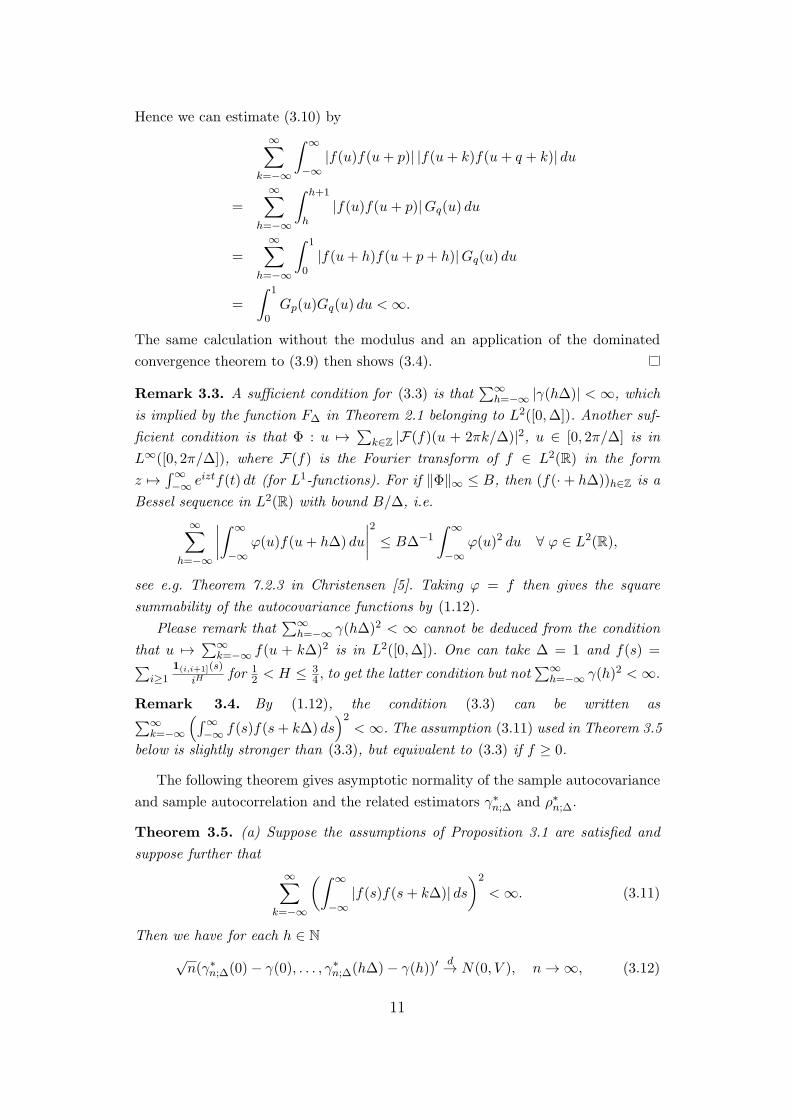
Remark 3.3. A sufficient condition for (3.3) is that∑∞

h=−∞ |γ(h∆)| < ∞, which

is implied by the function F∆ in Theorem 2.1 belonging to L2([0,∆]). Another suf-

ficient condition is that Φ : u 7→∑

k∈Z |F(f)(u + 2πk/∆)|2, u ∈ [0, 2π/∆] is in

L∞([0, 2π/∆]), where F(f) is the Fourier transform of f ∈ L2(R) in the form

z 7→∫∞−∞ eiztf(t) dt (for L1-functions). For if ∥Φ∥∞ ≤ B, then (f(·+ h∆))h∈Z is a

Bessel sequence in L2(R) with bound B/∆, i.e.

∞∑h=−∞

∣∣∣∣∫ ∞

−∞φ(u)f(u+ h∆) du

∣∣∣∣2 ≤ B∆−1

∫ ∞

−∞φ(u)2 du ∀ φ ∈ L2(R),

see e.g. Theorem 7.2.3 in Christensen [5]. Taking φ = f then gives the square

summability of the autocovariance functions by (1.12).

Please remark that∑∞

h=−∞ γ(h∆)2 < ∞ cannot be deduced from the condition

that u 7→∑∞

k=−∞ f(u + k∆)2 is in L2([0,∆]). One can take ∆ = 1 and f(s) =∑i≥1

1(i,i+1](s)

iHfor 1

2 < H ≤ 34 , to get the latter condition but not

∑∞h=−∞ γ(h)2 <∞.

Remark 3.4. By (1.12), the condition (3.3) can be written as∑∞k=−∞

(∫∞−∞ f(s)f(s+ k∆) ds

)2<∞. The assumption (3.11) used in Theorem 3.5

below is slightly stronger than (3.3), but equivalent to (3.3) if f ≥ 0.

The following theorem gives asymptotic normality of the sample autocovariance

and sample autocorrelation and the related estimators γ∗n;∆ and ρ∗n;∆.

Theorem 3.5. (a) Suppose the assumptions of Proposition 3.1 are satisfied and

suppose further that

∞∑k=−∞

(∫ ∞

−∞|f(s)f(s+ k∆)| ds

)2

<∞. (3.11)

Then we have for each h ∈ N√n(γ∗n;∆(0)− γ(0), . . . , γ∗n;∆(h∆)− γ(h))′

d→ N(0, V ), n→ ∞, (3.12)

11

where V = (vpq)p,q=0,...,h ∈ Rh+1,h+1 is the covariance matrix defined by

vpq = (η − 3)σ4∫ ∆

0gp;∆(u)gq;∆(u) du+

∞∑k=−∞

[γ(k∆)γ((k − p+ q)∆) + γ((k + q)∆)γ((k − p)∆)

]. (3.13)

(b) In addition to the assumptions of (a), assume that the function

u 7→∞∑

j=−∞|f(u+ j∆)|

is in L2([0,∆]). Denote by

γn;∆(j∆) = n−1n−j∑t=1

(Xt∆ −Xn;∆)(X(t+j)∆ −Xn;∆), j = 0, 1, . . . , n− 1,

the sample autocovariance, as defined in (1.4). Then we have for each h ∈ N√n(γn;∆(0)− γ(0), . . . , γn;∆(h∆)− γ(h))′

d→ N(0, V ), n→ ∞,

where V = (Vpq)p,q=0,...,h is defined by (3.13).

(c) For j ∈ N let ρ∗n;∆(j∆) = γ∗n;∆(j∆)/γ∗n;∆(0) and ρn(j∆) = γn;∆(j∆)/γn;∆(0),

the latter being the sample autocorrelation at lag j∆. Suppose that f is not almost

everywhere equal to zero. Then, under the assumptions of (a), we have for each

h ∈ N, that√n(ρ∗n;∆(∆)− ρ(∆), . . . , ρ∗n;∆(h∆)− ρ(h∆))′

d→ N(0,W ), n→ ∞, (3.14)

where W =W∆ = (wij;∆)i,j=1,...,h is given by

wij;∆ = wij;∆ +(η − 3)σ4

γ(0)2

∫ ∆

0

(gi;∆(u)− ρ(i∆)g0;∆(u)

)(gj;∆(u)− ρ(j∆)g0;∆(u)

)du,

and

wij;∆ =

∞∑k=−∞

(ρ((k + i)∆)ρ((k + j)∆) + ρ((k − i)∆)ρ((k + j)∆) + 2ρ(i∆)ρ(j∆)ρ(k∆)2

−2ρ(i∆)ρ(k∆)ρ((k + j)∆)− 2ρ(j∆)ρ(k∆)ρ((k + i)∆))

=

∞∑k=1

(ρ((k + i)∆) + ρ((k − i)∆)− 2ρ(i∆)ρ(k∆)

)×

(ρ((k + j)∆) + ρ((k − j)∆)− 2ρ(j∆)ρ(k∆)

)is given by Bartlett’s formula. If additionally the function u 7→

∑∞j=−∞ |f(u+ j∆)|

is in L2([0,∆]), then it also holds that

√n(ρn;∆(∆)− ρ(∆), . . . , ρn;∆(h∆)− ρ(h∆))′

d→ N(0,W ), n→ ∞. (3.15)

12

Proof. For simplicity in notation we assume again ∆ = 1 in this proof.

(a) Using Proposition 3.1 it follows as in the proof of Proposition 7.3.2 in [3],

that the claim is true if f has additionally compact support. For general f and

m ∈ N let fm := f1(−m,m). Hence we have that

n1/2(γ∗n;(m)(0)− γm(0), . . . , γ∗n;(m)(h)− γm(h))′d→ Ym, m→ ∞,

where γm is the autocovariance function of the process Xt;m =∫∞−∞ fm(t − s) dLs,

γ∗n;(m)(p) = n−1∑n

t=1Xt;mXt+p;m the corresponding autocovariance estimate, and

Ymd= N(0, Vm) with Vm = (vpq;m)p,q=0,...,h and

vpq;m = (η−3)σ4∫ 1

0gp;(m)(u)gq;(m)(u) du+

∞∑k=−∞

[γm(k)γm(k−p+q)+γm(k+q)γm(k−p)

].

Here, gp;(m)(u) =∑∞

k=−∞ fm(u+ k)fm(u+ k + p), u ∈ [0, 1].

Next, we want to show that limm→∞ Vm = V . Observe first that

gp;(m)(u) =

∞∑k=−∞

fm(u+k)fm(u+k+p) →∞∑

k=−∞f(u+k)f(u+k+p) = gp,1(u) =: gp(u)

almost surely in the variable u as m → ∞ by Lebesgue’s dominated convergence

theorem, since u 7→∑∞

k=−∞ |f(u+k)f(u+k+p)| is in L2([0, 1]) by (3.2) and hence

is almost surely finite. Further we have

|gp;(m)(u)| ≤∞∑

k=−∞|f(u+ k)f(u+ k + p)|

uniformly in u and m, so that again by the dominated convergence theorem we have

that gp;(m) → gp in L2([0, 1]) as m→ ∞. Next, observe that

|γm(k)| ≤∫ ∞

−∞|f(s)f(s+ k)| ds ∀ m ∈ N ∀ k ∈ Z.

Since limm→∞ γm(k) = γ(k) for every k ∈ Z, it follows from the dominated con-

vergence theorem and (3.11) that (γm(k))k∈Z converges in l2(Z) to (γ(k))k∈Z. This

together with the convergence of gp;(m) gives the desired limm→∞ Vm = V , so that

Ymd→ Y, m→ ∞,

where Yd= N(0, V ). Finally, that

limm→∞

lim supn→∞

P (n1/2|γ∗n;(m)(p)−γm(p)−γ∗(p)+γ(p)| > ε) = 0 ∀ ε > 0, p ∈ {0, . . . , h}

follows as in Equation (7.3.9) in [3]. An application of a variant of Slutsky’s theorem

(cf. [3], Proposition 6.3.9) then gives the claim.

(b) This follows as in the proof of Proposition 7.3.4 in [3]. One only has to observe

13

that by Theorem 2.1,√nXn;1 converges in distribution to a normal random variable

as n→ ∞. In particular, Xn;1 must converge to 0 in probability as n→ ∞.

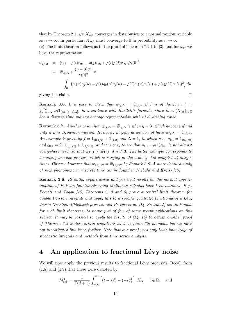
(c) The limit theorem follows as in the proof of Theorem 7.2.1 in [3], and for wij we

have the representation

wij;∆ = (vij − ρ(i)v0j − ρ(j)vi0 + ρ(i)ρ(j)v00)/γ(0)2

= wij;∆ +(η − 3)σ4

γ(0)2×∫ 1

0

(gi(u)gj(u)− ρ(i)g0(u)gj(u)− ρ(j)gi(u)g0(u) + ρ(i)ρ(j)g0(u)

2)du,

giving the claim.

Remark 3.6. It is easy to check that wij;∆ = wij;∆ if f is of the form f =∑∞i=−∞ ψi1(i∆,(i+1)∆], in accordance with Bartlett’s formula, since then (Xt∆)t∈Z

has a discrete time moving average representation with i.i.d. driving noise.

Remark 3.7. Another case when wij;∆ = wij;∆ is when η = 3, which happens if and

only if L is Brownian motion. However, in general we do not have wij;∆ = wij;∆.

An example is given by f = 1(0,1/2] + 1(1,2] and ∆ = 1, in which case g1;1 = 1(0,1/2]

and g0;1 = 2 ·1(0,1/2]+1(1/2,1], and it is easy to see that g1;1− ρ(1)g0;1 is not almost

everywhere zero, so that w11;1 = w11;1 if η = 3. The latter example corresponds to

a moving average process, which is varying at the scale 12 , but sampled at integer

times. Observe however that w11;1/2 = w11;1/2 by Remark 3.6. A more detailed study

of such phenomena in discrete time can be found in Niebuhr and Kreiss [13].

Remark 3.8. Recently, sophisticated and powerful results on the normal approx-

imation of Poisson functionals using Malliavan calculus have been obtained. E.g.,

Peccati and Taqqu [15, Theorems 2, 3 and 5] prove a central limit theorem for

double Poisson integrals and apply this to a specific quadratic functional of a Levy

driven Ornstein–Uhlenbeck process, and Peccati et al. [14, Section 4] obtain bounds

for such limit theorems, to name just of few of some recent publications on this

subject. It may be possible to apply the results of [14, 15] to obtain another proof

of Theorem 3.5 under certain conditions such as finite 6th moment, but we have

not investigated this issue further. Note that our proof uses only basic knowledge of

stochastic integrals and methods from time series analysis.

4 An application to fractional Levy noise

We will now apply the previous results to fractional Levy processes. Recall from

(1.8) and (1.9) that these were denoted by

M1t;d :=

1

Γ(d+ 1)

∫ ∞

−∞

[(t− s)d+ − (−s)d+

]dLs, t ∈ R, and

14

M2t;d =

∫ ∞

−∞

[|t− s|d − |s|d

]dLs, t ∈ R,

respectively, and the corresponding fractional Levy noises based on increments of

length ∆ > 0 by

Xit =M i

t;d −M it−∆;d, t ∈ R, i = 1, 2.

Hence the fractional Levy noises are Levy driven moving average processes with

kernel functions

f1d,∆(s) =1

Γ(d+ 1)

(sd+ − (s−∆)d+

), s ∈ R,

and

f2d,∆(s) = |s|d − |s−∆|d, s ∈ R,

respectively. Neither f1d,∆ nor f2d,∆ are in L1(R), so Theorem 2.1 cannot be applied

because of Remark 2.3. Please note that for the same reason the assumptions for

(b) of Theorem 3.5 and for (3.15) are not fulfilled.

For simplicity in notation we assume ∆ = 1, and drop the subindex ∆. Although

the fractional noises Xi have different distributions for i = 1 and i = 2, they are

both stationary with the autocovariance

E(Xit+hX

it) = γXi(h) =

Ci(d)σ2

2

(|h+ 1|2d+1 − 2|h|2d+1 + |h− 1|2d+1

), (4.1)

where Ci(d) is a normalising multiplicative constant depending on d. Both processes

Xi are infinitely divisible and of moving average type, hence we know from [4, 8]

that (Xit)t∈Z is mixing in the ergodic-theoretic sense. For fixed h ∈ Z, define the

function

F : RZ → R, (xn)n∈Z 7→ x0xh.

If T denotes the forward shift operator, then

F (T k(Xit)t∈Z) = Xi

kXik+h,

and from Birkhoff’s ergodic theorem (e.g. Ash and Gardner [1], Theorems 3.3.6 and

3.3.10) we know that

1

n

n∑k=1

XikX

ik+h → E

(F ((Xi

t)t∈Z))= EX i

0Xih, n→ ∞,

for i = 1, 2, and the convergence is almost sure and in L1 ([1], Theorems 3.3.6 and

3.3.7). Hence, with γ∗n = γ∗n;1 as defined in (1.6),

limn→∞

γ∗n(h) =Ci(d)σ2

2

(|h+ 1|2d+1 − 2|h|2d+1 + |h− 1|2d+1

)a.s.

15

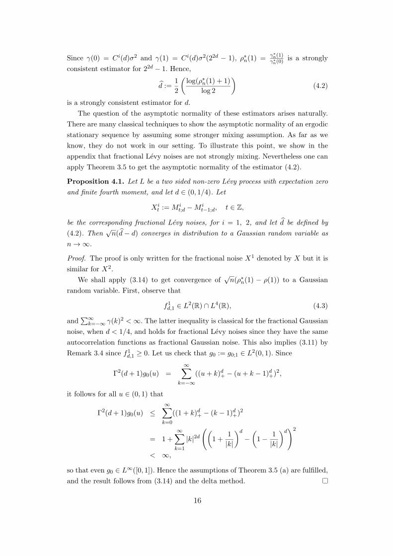
Since γ(0) = Ci(d)σ2 and γ(1) = Ci(d)σ2(22d − 1), ρ∗n(1) = γ∗n(1)

γ∗n(0)

is a strongly

consistent estimator for 22d − 1. Hence,

d :=1

2

(log(ρ∗n(1) + 1)

log 2

)(4.2)

is a strongly consistent estimator for d.

The question of the asymptotic normality of these estimators arises naturally.

There are many classical techniques to show the asymptotic normality of an ergodic

stationary sequence by assuming some stronger mixing assumption. As far as we

know, they do not work in our setting. To illustrate this point, we show in the

appendix that fractional Levy noises are not strongly mixing. Nevertheless one can

apply Theorem 3.5 to get the asymptotic normality of the estimator (4.2).

Proposition 4.1. Let L be a two sided non-zero Levy process with expectation zero

and finite fourth moment, and let d ∈ (0, 1/4). Let

Xit :=M i

t;d −M it−1;d, t ∈ Z,

be the corresponding fractional Levy noises, for i = 1, 2, and let d be defined by

(4.2). Then√n(d − d) converges in distribution to a Gaussian random variable as

n→ ∞.

Proof. The proof is only written for the fractional noise X1 denoted by X but it is

similar for X2.

We shall apply (3.14) to get convergence of√n(ρ∗n(1) − ρ(1)) to a Gaussian

random variable. First, observe that

f1d,1 ∈ L2(R) ∩ L4(R), (4.3)

and∑∞

k=−∞ γ(k)2 <∞. The latter inequality is classical for the fractional Gaussian

noise, when d < 1/4, and holds for fractional Levy noises since they have the same

autocorrelation functions as fractional Gaussian noise. This also implies (3.11) by

Remark 3.4 since f1d,1 ≥ 0. Let us check that g0 := g0;1 ∈ L2(0, 1). Since

Γ2(d+ 1)g0(u) =

∞∑k=−∞

((u+ k)d+ − (u+ k − 1)d+)2,

it follows for all u ∈ (0, 1) that

Γ2(d+ 1)g0(u) ≤∞∑k=0

((1 + k)d+ − (k − 1)d+)2

= 1 +∞∑k=1

|k|2d((

1 +1

|k|

)d

−(1− 1

|k|

)d)2

< ∞,

so that even g0 ∈ L∞([0, 1]). Hence the assumptions of Theorem 3.5 (a) are fulfilled,

and the result follows from (3.14) and the delta method.

16

If d ≥ 1/4 then∑∞

k=−∞ γ(k)2 = ∞, since fractional Levy noises have the same

autocorrelation functions as the fractional Gaussian noise. Hence we consider

Zit = Xi

t −Xit−1, t ∈ Z,

for which it holds∑∞

k=−∞ γZi(k)2 <∞. We conclude from Birkhoff’s ergodic theo-

rem that

γ∗n,Z(h) :=1

n

n∑k=2

ZikZ

ik+h

is a strongly consistent estimator of

E(Zi0Z

ih) =

Ci(d)σ2

2

(−|h+ 2|2d+1 + 4|h+ 1|2d+1 − 6|h|2d+1 + 4|h− 1|2d+1 − |h− 2|2d+1

).

Therefore ρ∗n,Z(1) =γ∗n,Z(1)

γ∗n,Z(0) is a strongly consistent estimator for ϕ(d) = ρZi(1) =

−32d+1+4·22d+1−78−22d+2 . It turns out that ϕ is increasing on (0, 1/2). Therefore we can

define the estimator

d := ϕ−1(ρ∗n,Z(1)). (4.4)

Proposition 4.2. Under the assumptions of Proposition 4.1, but with d ∈ (0, 1/2)

rather than d ∈ (0, 1/4), let d be defined by (4.4). Then√n(d − d) converges in

distribution to a Gaussian random variable as n→ ∞.

Proof. The proof is only written for the fractional noise X1 denoted by X but it is

similar for X2. Let us remark that Zt = Z1t =

∫∞−∞ f1d,1(t− s) dLs, where

f1d,1(s) = f1d,1(s)− f1d,1(s− 1).

To apply Theorem 3.5, we have to check that

f1d,1(s) ∈ L2(R) ∩ L4(R),

which is obvious from (4.3). Moreover we already know that∑∞

k=−∞ γZi(k)2 <∞.

This time, however, the kernel function f1d,1 is not nonnegative, but it is easy to see

that |f1d,1(t)| ≤ Cmin(1, |t|d−2) and hence that∫ ∞

−∞|f1d,1(t) f1d,1(t+ k)| dt ≤ C ′min(1, |k|d−1), ∀ k ∈ Z,

for some constants C,C ′, giving (3.11). Finally,

Γ2(d+ 1)g0(u) =∞∑

k=−∞((u+ k)d+ + (u+ k − 2)d+ − 2(u+ k − 1)d+)

2,

and estimating the summands separately for k < 0, k = 0, 1 and k ≥ 2 we obtain

for u ∈ [0, 1]

Γ2(d+ 1)g0(u) ≤ 1 + (2d + 2)2 +∞∑k=2

(kd − (k − 1)d)2

< ∞,

17

so that g0 ∈ L∞([0, 1]) ⊂ L2([0, 1]). The claim now follows from Theorem 3.5, using

(3.14) and the delta method.

Let us now compare the asymptotic variances of the estimators d and d defined by

(4.2) and (4.4), respectively, for the fractional noise X = X1, under the assumptions

of Proposition 4.1 with d ∈ (0, 1/4). By Propositions 4.1 and 4.2, we have

√n(d− d)

d→ N(0, v(d)) and√n(d− d)

d→ N(0, v(d))

as n→ ∞, where v(d) and v(d) are the asymptotic variances of d and d, respectively.

Denote the Levy measure of L by ν, its Gaussian variance by A, σ2 := EL21 and

η := σ−4EL41. By the proof of Lemma 3.2, (η − 3)σ4 =

∫R x

4 ν(dx) and σ2 =

A+∫R x

2 ν(dx). It then follows from Theorem 3.5 (c) and the delta method that

v(d) = b(d) +

∫R x

4 ν(dx)

(A+∫R x

2 ν(dx))2c(d) and v(d) = b(d) +

∫R x

4 ν(dx)

(A+∫R x

2 ν(dx))2c(d)

for suitable b(d), c(d), b(d), c(d) ≥ 0. Here the terms b(d) and b(d) correspond to

the contribution of Bartlett’s formula to the asymptotic variance, and c(d) and

c(d) correspond to the correction term to Bartlett’s formula in Theorem 3.5 (c).

Obviously, v(d) = b(d) and v(d) = b(d) when L is a Brownian motion, but they

differ for general Levy processes. Table 1 gives the values of b(d), c(d), b(d), c(d)

for various values of d, along with v(d) and v(d) when∫R x4 ν(dx)

(A+∫R x2 ν(dx))2

= 100, which

happens for example when A = 0 and ν = 0.01δ1, i.e. when L is a centered Poisson

process with parameter 0.01 with drift. It turns out that for all considered values of d

the correction terms c(d) and c(d) are small compared to b(d) and c(d), respectively,

but make a significant effect for large values of∫R x4 ν(dx)

(A+∫R x2 ν(dx))2

. The correction term

c(d) is smaller than c(d) for all considered values of d, while the Bartlett contribution

term b(d) is smaller than b(d) only if d ≤ 0.242 and explodes as d approaches 1/4,

while b(d) stays bounded. Still, if∫R x4 ν(dx)

(A+∫R x2 ν(dx))2

= 100, the asymptotic variance v(d)

of d is still smaller than the asymptotic variance v(d) of d when d ∈ {0.243, 0.244}due to the effect of the correction terms c(d) and c(d), respectively. Summing up,

the estimator d has a smaller asymptotic variance than d for all considered values

of d ≤ 0.242, but its asymptotic variance explodes as d approaches 0.25.

A Appendix

In this appendix we show that fractional noise driven by a Levy process with

finite fourth moment is not strongly mixing. Let us first recall that a stationary

sequence (Yn)n∈Z is strongly mixing (or α-mixing) if limn→∞ αY (n) = 0, where

αY (n) = sup{|P (A∩B)−P (A)P (B)|, A ∈ σ(Yk, k ≤ 0), B ∈ σ(Yk, k ≥ n)}.

18

d b(d) c(d) b(d) c(d) b(d) + 100c(d) b(d) + 100c(d)

0.025 0.4985 0.0002 1.6295 0.0003 0.5173 1.6573

0.050 0.4782 0.0006 1.6683 0.0011 0.5442 1.7775

0.075 0.4602 0.0013 1.7075 0.0024 0.5895 1.9493

0.100 0.4455 0.0020 1.7470 0.0042 0.6446 2.1712

0.125 0.4358 0.0027 1.7868 0.0066 0.7035 2.4422

0.150 0.4350 0.0033 1.8267 0.0093 0.7638 2.7610

0.175 0.4515 0.0038 1.8667 0.0126 0.8294 3.1263

0.200 0.5103 0.0041 1.9068 0.0163 0.9224 3.5363

0.225 0.7373 0.0043 1.9468 0.0204 1.1664 3.9889

0.240 1.4764 0.0043 1.9707 0.0231 1.9073 4.2797

0.241 1.6150 0.0043 1.9735 0.0233 2.0458 4.3022

0.242 1.7884 0.0043 1.9751 0.0235 2.2190 4.3221

0.243 2.0117 0.0043 1.9767 0.0237 2.4422 4.3422

0.244 2.3097 0.0043 1.9783 0.0238 2.7400 4.3622

0.249 12.767 0.0043 1.9862 0.0248 13.196 4.4635

0.2499 125.76 0.0043 1.9864 0.0249 126.19 4.4791

Table 1: The asymptotic variances b(d) and b(d) of d and d according to Bartlett’s formula when

L is Brownian motion, the correction terms c(d) and c(d) when L is not Brownian motion, and

the asymptotic variances v(d) = b(d) +∫R x4 ν(dx)

(A+∫R x2 ν(dx))2

c(d) and v(d) = b(d) +∫R x4 ν(dx)

(A+∫R x2 ν(dx))2

c(d)

when∫R x4 ν(dx)

(A+∫R x2 ν(dx))2

= 100.

In the case of fractional noise X, we know the mixing property in the ergodic-

theoretic sense. However, fractional Levy noise is not strongly mixing as shown

in the following theorem:

Theorem A.1. Let L be a two sided non-zero Levy process with expectation

zero and finite fourth moment, and let d ∈ (0, 1/2). Let

X it := M i

t;d −M it−1;d, t ∈ Z,

be the corresponding fractional Levy noises, for i = 1, 2. Then X1 and X2 are

not strongly mixing.

Proof. The proof is only written for fractional noise X2 denoted by X but it

is similar for X1. We also write Mt;d = M2t;d. Since L has finite fourth moment

and since the kernel function of fractional noise is in L2(R) ∩ L4(R), we have

E|X0|4 < ∞. Since∑m

i=1Xi = Mm;d we have

Var (m∑i=1

Xi) = Var (Mm;d) = Cm2d+1 → ∞ as m → ∞

19

for some constant C. Denote fm(s) := |m− s|d − |s|d. Then by Lemma 3.2,

E

∣∣∣∣∣m∑i=1

Xi

∣∣∣∣∣4

= E|Md(m)|4 = (η − 3)σ4

∫Rf 4m(s)ds+ 3σ4

(∫Rf 2m(s)ds

)2

.

Since (∫Rf 2m(s) ds

)2

= Cm4d+2 and

∫Rf 4m(s) ds ≤ C ′m4d+1

for positive constants C, C ′, we have

supm∈N

(Var (

m∑i=1

Xi)

)−2

E

∣∣∣∣∣m∑i=1

Xi

∣∣∣∣∣4 < ∞.

Now if X were strongly mixing, then it would follow from Proposition 34 in

[12] that

(Var (Mn;d))−1/2 (M⌊nt⌋;d)t∈[0,1]

converges weakly to a standard Brownian motion in the Skorohod spaceD[0, 1]

as n → ∞. On the other hand, owing to the asymptotic self-similarity of frac-

tional Levy processes (Proposition 3.1 in [2]), it is known that n−d−1/2(M⌊nt⌋;d)t∈[0,1]

converges weakly to a fractional Brownian motion with Hurst exponent d+1/2

as n → ∞. Hence we obtain a contradiction and X2 cannot be strongly mix-

ing.

Acknowledgement

Major parts of this research where carried out while AL was visiting the In-

stitut de Mathematiques de Toulouse as guest professor in 2008 and 2009. He

takes pleasure in thanking them for the kind hospitality and their generous

financial support. We also would like to thank the anonymous referee and the

Associate Editor for their careful reading of the manuscript and their helpful

comments, which helped to improve the manuscript.

References

[1] R.B. Ash and M.F. Gardner. Topics in Stochastic Processes. Academic

Press [Harcourt Brace Jovanovich Publishers], New York, 1975. Proba-

bility and Mathematical Statistics, Vol. 27.

[2] A. Benassi, S. Cohen, and J. Istas. On roughness indices for fractional

fields. Bernoulli, 10(2):357–373, 2004.

20

[3] P.J. Brockwell and R.A. Davis. Time Series: Theory and Methods.

Springer Series in Statistics. Springer-Verlag, New York, 1987.

[4] S. Cambanis, K. Podgorski, and A. Weron. Chaotic behavior of infinitely

divisible processes. Studia Math., 115(2):109–127, 1995.

[5] O. Christensen. An Introduction to Frames and Riesz Bases. Applied

and Numerical Harmonic Analysis. Birkhauser Boston Inc., Boston, MA,

2003.

[6] S. Cohen. Fractional Levy fields. In: S. Cohen, A. Kutznetsov, A. Kypri-

anou, V. Rivero: Levy Matters II. Lecture Notes in Mathematics, Vol.

2061, pp. 1–94. Springer-Verlag, 2013.

[7] R.A. Davis and Th. Mikosch. The sample autocorrelations of heavy-tailed

processes with applications to ARCH. Ann. Statist., 26(5):2049–2080,

1998.

[8] F. Fuchs and R. Stelzer. Mixing conditions for multivariate infinitely

divisible processes with an application to mixed moving averages and the

sup ou stochastic volatility model. ESAIM Probab. Stat. To appear.

ESAIM:PS.doi 10.1051/ps2011158.

[9] E. J. Hannan. The asymptotic distribution of serial covariances. Ann.

Statist., 4(2):396–399, 1976.

[10] I. A. Ibragimov and Yu. V. Linnik. Independent and Stationary Sequences

of Random Variables. Wolters-Noordhoff Publishing, Groningen, 1971.

With a supplementary chapter by I. A. Ibragimov and V. V. Petrov,

Translation from the Russian, edited by J. F. C. Kingman.

[11] T. Marquardt. Fractional Levy processes with an application to long

memory moving average processes. Bernoulli, 12(6):1099–1126, 2006.

[12] F. Merlevede, M. Peligrad, and S. Utev. Recent advances in invariance

principles for stationary sequences. Probab. Surveys, 3:1–36, 2006.

[13] T. Niebuhr and J.-P. Kreiss. Asymptotics for autocovariances and inte-

grated periodograms for linear processes observed at lower frequencies.

Preprint, 2012.

[14] G. Peccati, J.-L. Sole, M.S. Taqqu, and F. Utzet. Stein’s method and

normal approximation of Poisson functionals. Ann. Probab., 37:2231–

2261, 2010.

[15] G. Peccati and M.S. Taqqu. Central limit theorems for double Poisson

integrals. Bernoulli, 14:791–821, 2008.

21