IN DEGREE PROJECT TECHNOLOGY,FIRST CYCLE, 15 CREDITS

, STOCKHOLM SWEDEN 2016

A comparative study between a simulated annealing and a genetic algorithm for solving a university timetabling problem

JONAS DAHL

RASMUS FREDRIKSON

KTH ROYAL INSTITUTE OF TECHNOLOGYSCHOOL OF COMPUTER SCIENCE AND COMMUNICATION

A comparative study between a simulatedannealing and a genetic algorithm for solving a

university timetabling problem

En jämförande studie mellan en algoritm baserad på simulerad glödgning ochen genetisk algoritm för att lösa ett universitetsschemaläggningsproblem

JONAS DAHLRASMUS FREDRIKSON

Degree Project in Computer Science, DD143XSupervisor: Dilian GurovExaminer: Örjan Ekeberg

CSC, KTH. Stockholm, Sweden. May 11, 2016.

iii

Abstract

The university timetabling problem is an NP-complete problem which schoolsall over the world face every semester. The aim of the problem is to schedulesets of events such as lectures and seminars into certain time slots withoutviolating numerous specified constraints. This study aimed to automate thisprocess with the help of simulated annealing and compare the results with agenetic algorithm.

The input data sets were inspired by the Royal Institute of Technology inStockholm. The results showed a great run time difference between the twoalgorithms where the simulated annealing performed much better. They alsoshowed that even though the simulated annealing algorithm was better duringall stages, the genetic algorithm had a much better performance in early stagesthan it had in latter. This led to the conclusion that a more optimized, hybridalgorithm could be created from the two algorithms provided that the geneticalgorithm could benefit from the improvements suggested in previous research.

iv

Sammanfattning

Universitetsschemaläggningsproblemet är ett NP-fullständigt problem somskolor över hela världen måste hantera innan varje termin. Syftet med proble-met är att schemalägga händelser, såsom föreläsningar och seminarier, utan attbryta flertalet fördefinierade villkor.

Denna studie hade som mål att automatisera denna process med hjälp avalgoritmkonstuktionsmetoden simulerad glödgning och sedan jämföra resulta-tet med en genetisk algoritm. De datamängder som användes är inspirerade avden verkliga situationen på KTH. Resultaten visar stora tidsmässiga skillnaderdär algoritmen baserad på simulerad glödgning går snabbare. De visar dockockså att den genetiska algoritmen har en bättre prestanda i tidigare stadierän i senare. Detta ledde till slutsatsen att en mer optimerad hybridalgoritmkan skapas av de två algoritmerna, förutsatt att den genetiska algoritmen kandra nytta av förbättringar som föreslagits i tidigare forskning.

Contents

1 Introduction 11.1 Purpose . . . . . . . . . . . . . . . . . . . . . . . . . . . . . . . . . . 21.2 Problem statement . . . . . . . . . . . . . . . . . . . . . . . . . . . . 2

1.2.1 Limitations . . . . . . . . . . . . . . . . . . . . . . . . . . . . 21.3 Outline . . . . . . . . . . . . . . . . . . . . . . . . . . . . . . . . . . 3

2 Background 52.1 The university timetabling problem . . . . . . . . . . . . . . . . . . . 5

2.1.1 Time complexity . . . . . . . . . . . . . . . . . . . . . . . . . 52.2 Constraint based algorithms . . . . . . . . . . . . . . . . . . . . . . . 5

2.2.1 Three different classes of constraint based algorithms . . . . . 62.3 Meta-heuristic algorithms . . . . . . . . . . . . . . . . . . . . . . . . 6

2.3.1 Genetic algorithm . . . . . . . . . . . . . . . . . . . . . . . . 72.3.2 Simulated annealing . . . . . . . . . . . . . . . . . . . . . . . 7

3 Method 93.1 Test approach . . . . . . . . . . . . . . . . . . . . . . . . . . . . . . . 9

3.1.1 Environment . . . . . . . . . . . . . . . . . . . . . . . . . . . 93.2 Algorithms . . . . . . . . . . . . . . . . . . . . . . . . . . . . . . . . 10

3.2.1 Data structures . . . . . . . . . . . . . . . . . . . . . . . . . . 103.2.2 Genetic algorithm . . . . . . . . . . . . . . . . . . . . . . . . 103.2.3 Simulated annealing . . . . . . . . . . . . . . . . . . . . . . . 11

3.3 Data sets . . . . . . . . . . . . . . . . . . . . . . . . . . . . . . . . . 123.4 Constraints . . . . . . . . . . . . . . . . . . . . . . . . . . . . . . . . 13

3.4.1 Assessment . . . . . . . . . . . . . . . . . . . . . . . . . . . . 14

4 Results 15

5 Discussion 215.1 Time complexity . . . . . . . . . . . . . . . . . . . . . . . . . . . . . 215.2 Main differences between the two algorithms . . . . . . . . . . . . . 21

5.2.1 Basic local search may be sufficient . . . . . . . . . . . . . . . 225.3 Reliability . . . . . . . . . . . . . . . . . . . . . . . . . . . . . . . . . 225.4 Improvements . . . . . . . . . . . . . . . . . . . . . . . . . . . . . . . 22

v

vi CONTENTS

5.4.1 Refined fitness function . . . . . . . . . . . . . . . . . . . . . 225.4.2 Soft constraints . . . . . . . . . . . . . . . . . . . . . . . . . . 23

6 Conclusions 25

Bibliography 27

A Source code 29

B Data sets 31B.1 XL - Extra large . . . . . . . . . . . . . . . . . . . . . . . . . . . . . 31B.2 L - Large . . . . . . . . . . . . . . . . . . . . . . . . . . . . . . . . . 33B.3 M - Medium . . . . . . . . . . . . . . . . . . . . . . . . . . . . . . . . 35B.4 S - Small . . . . . . . . . . . . . . . . . . . . . . . . . . . . . . . . . 36B.5 XS - Extra small . . . . . . . . . . . . . . . . . . . . . . . . . . . . . 37

Chapter 1

Introduction

Each day we face the problem of getting our schedule to align with other people’s.Scheduling is in general a very difficult problem that can be found everywhere: atuniversities and high schools, in public transport, at hospitals and a vast numberof other institutions.

Universities all over the world need to solve the scheduling problem at least oncebefore each semester. If done manually, massive amount of time need to be spenton making a suitable schedule. The schedule needs to fulfill several constraints.Common constraints are that only one teacher can teach one class at one specifictime, a room can only be occupied by one class at a time and students should nothave more than one class each time period. These constraints are often divided intohard and soft constraints. [4] The hard constraints are not allowed to be violated,while the soft constraints may be violated, but with the setback of a less optimalschedule.

Due to the huge amount of time and money spent on scheduling manually, therehave been numerous attempts to automate this task with the help of computers.Research has shown that this problem is most commonly NP-complete [2], howeverthis of course depends on how many and how complex the constraints are. Due tothe difficulty of the problem and the many different constraints, there is no generalalgorithm which will find the optimal solution for every timetable problem.

To get around this problem, several optimization algorithms have been imple-mented. These algorithms are mostly meta-heuristic and range from local search al-gorithms like tabu search [14] and simulated annealing [9] to evolutionary algorithmslike particle swarm optimization [5] and genetic algorithms [13]. The reason for themany different algorithms being implemented is because of the complex nature ofthe problem. Almost every school has different constraints and pre-conditions whichneed to be fulfilled. The evolutionary algorithms mostly performs better in the earlystages of the process whereas the local search algorithms performs better in the latestages. This has led to the creation of many hybrid algorithms [11] which use evo-lutionary algorithms to narrow down the search space and local search algorithmsto find the best solution in that space.

1

2 CHAPTER 1. INTRODUCTION

The original genetic algorithm was created by John Holland [6] in the early1970’s. The genetic algorithm is inspired by the evolution of life and was made tomimic some of life’s evolutionary processes. It is an adaptive heuristic algorithmwhich uses an intelligent random search to find a solution to a problem. The in-telligent random search is however by no means random. Instead it uses previousacquired information to find a more suitable candidate solution in the search space,thus fulfilling Darwin’s quote "Survival of the fittest".

The simulated annealing algorithm construction method was first proposed in1983. [9] Annealing is a process in metallurgy where a metal is slowly cooled tomake it stronger by reaching a low energy state. Based on this process the simu-lated annealing algorithm finds a solution to a problem. The simulated annealingalgorithm is like the genetic algorithm also a heuristic algorithm.

Both algorithms have already previously been implemented and have successfullysolved the university timetabling problem, for example by Andersson [1] as well asPertoft and Yamazaki [13].

1.1 PurposePrevious research has shown that evolutionary algorithms are good for exploring thewhole search space. [7] As this might be the case for timetabling problems, a geneticalgorithm is interesting for a comparison. Renman and Fristedt [14] presents a tabusearch that does not perform as good as the genetic algorithm they compared it with.They do however state that there are other kinds of local searches, like simulatedannealing, that might perform better than the genetic algorithm. Therefore, thisstudy compares a simulated annealing algorithm with a genetic algorithm.

Hybrids of several different algorithms are commonly used nowadays to solve thetimetabling problem. [14] Therefore it would be interesting to investigate whetheror not the two algorithms would perform better as a hybrid than by themselves.

1.2 Problem statementThe main study will be to investigate which of the genetic algorithm constructed byPertoft and Yamazaki [13] and the simulated annealing based algorithm constructedby the authors of this report, is fastest when executed on five different data sets.

The study will also investigate the potential benefit of creating a hybrid of thetwo algorithms.

1.2.1 Limitations

This study does not attempt to compare genetic algorithms with simulated anneal-ing algorithms in general. The result of this study focuses on the differences betweenthe two specific implementations presented in chapter 3. However, the conclusionscan be used as an indication of how well implementations based on these heuristics

1.3. OUTLINE 3

will perform. There are also other types of algorithms, for example hybrid solvers[11], that combine solution methods to create faster and better algorithms. Thisstudy does only compare two specific kinds of solvers.

The data sets used as input to the algorithms are similar to the data sets usedby Pertoft and Yamazaki [13], extended with a fifth data set inspired by the realcourse scheduling problem at the Royal Institute of Technology, KTH.

The algorithms use a common fitness function and the problem will be consideredsolved when the fitness value of a solution has reached 0.

The genetic algorithm that originally was written by Pertoft and Yamazaki [13],does not take soft constraints into consideration. Therefore, the simulated annealingalgorithm does not implement these either. Essentially, the algorithms share fitnessfunction to make them comparable. Due to this fact, an optimal solution will notbe found, only an accepted.

1.3 OutlineThe report is divided into six chapters. The first chapter introduces the subject,the problem statement and the purpose of the study. In chapter 2, Background,the university timetabling problem and the two different algorithms are describedin general, whereas the third chapter, Method, consists of how the two specificalgorithms are implemented. The results are shown in the fourth chapter and arediscussed in the fifth, Discussion. Lastly the results are concluded in the finalchapter, Conclusion.

Chapter 2

Background

This chapter starts with a presentation of the university timetabling problem, whichis followed up by a section explaining constraints and three different classes ofalgorithms. Two algorithms for solving the university timetabling problem are lastlypresented.

2.1 The university timetabling problem

The university timetabling problem is as aforementioned in the introduction, anNP-complete problem. The problem could be explained as followed: given a certainset of data and constraints a solution should be made which violates as few of theconstraints as possible. The data set usually consists of the teachers, students androoms and their capacity on the school. A room could also have certain abilities.For example, only laboratories can hold laboratory classes.

2.1.1 Time complexity

When the density of events increases and the amount of time slots are constant,the run time is increased more than linearly. Since the data sets and constraintsdiffer so much between schools and because of the time complexity, an effective,general algorithm solver is infeasible to create. The problem is, however, consideredNP-complete when using non-trivial constraints. [2]

2.2 Constraint based algorithms

Constraints can be divided into soft and hard constraints. [4] Hard constraintscannot be violated and should only be vital such as that a teacher can only haveone class at a time and a room cannot hold more people than its capacity. Softconstraints consist of less important constraints such as: a student should not havelong free time between classes or too many classes the same day. These constraints

5

6 CHAPTER 2. BACKGROUND

can be violated in favor of not violating a hard constraint, however with the resultof a less optimal solution.

2.2.1 Three different classes of constraint based algorithms

There are three main classes of university timetabling algorithms according to Lewis[10]: “one-stage optimisation algorithms, two-stage optimisation algorithms, and al-gorithms that allow relaxations”. Each of the algorithm types has its own advantagesand disadvantages, and they have different efficiency for different kinds of problems.The algorithm that allows relaxation is redundant for this study and is thereforenot described.

One-stage algorithms

The one-stage algorithms have one clear goal and a function returning a value ofhow close to the goal the solution is. Therefore, these algorithms can break bothhard and soft constraints. High values are assigned to the hard constraints toavoid breaking them, thus forcing the algorithm to choose a solution which at worseonly breaks the soft constraints. This category contains simple simulated annealingattempts and local search implementations, provided they are made in a way sothat they do not start with a valid solution. [10]

Two-stage algorithms

The two-stage algorithms have two phases. In the first, only hard constraints aretaken into account. After the first stage, a valid solution will exist. However, thesolution found after stage one is not guaranteed to be optimized at all. The secondstage is about refining the solution from the first stage to make it closer to theoptimal solution. This stage also uses a function as in one-stage algorithms, but donot need the hard constraints to be weighted with a very high weight to be takeninto account. This is because the solution during stage two only will be refined, andnever invalid. The simulated annealing can be used as an example in this categorytoo, if a valid solution is created before running the actual annealing. [10]

2.3 Meta-heuristic algorithms

Many different algorithms have been constructed to solve the university timetablingproblem. These are most commonly meta-heuristic algorithms using the power ofevolution such as the genetic algorithm or local search such as simulated annealing.These kinds of algorithms calculate an approximate solution rather than the optimalone. This is to severely decrease the run time of the program and still get anacceptable solution.

2.3. META-HEURISTIC ALGORITHMS 7

2.3.1 Genetic algorithm

A genetic algorithm starts with a set of random solutions to the problem. The initialsolution is randomized and therefore crude. Each solution is called a chromosomeand consists of several genes which are values corresponding to certain properties inthe solution. These genes can then be used to control the fitness of the chromosome.Based on the chromosomes’ fitness, they are crossed with each other to create a newoffspring. These offsprings are then randomly mutated to create a bigger searchspace. When an offspring matches a specified fitness condition, this means anacceptable solution has been found and the algorithm terminates. [12] There aretwo main stages in the genetic algorithm: the selection and the crossover.

Selection

When to select which chromosomes are to be crossed there are a few differentways. Some of these are elitism selection, roulette-wheel selection and tournamentselection. [13]

Crossover

It may vary which genes are carried over when two chromosomes are being crossed.To decide this there are few different methods. Some of them are single pointcrossover, two point crossover and uniform crossover. [13]

2.3.2 Simulated annealing

Simulated annealing is based on neighborhood search with the special property ofsometimes accepting a worse solution to avoid getting caught in a local optimumand instead finding the global one. [8] The idea of simulated annealing is inspiredby the annealing process in metal work. The colder a metal is, the more stable itsshape is. To change the shape of the metal it is heated up and then processed whileit is cooling down, ultimately freezing its shape until reheated.

Simulated annealing works in a similar way, where it has a temperature vari-able controlling the heating process. The temperature variable is initially set to ahigh value and is then slowly decreased while the algorithm runs. The higher thetemperature is, the more probable the algorithm is to choose a worse solution thanthe current one. This gives the algorithm the chance of avoiding getting stuck in alocal optimum early on. As the temperature decreases, so does the chances of thealgorithm choosing a worse solution, which in the end leads to a local search in amuch more narrow search space and hopefully finding a, close to, optimal solution.

Algorithms using only downhill search have a very large chance of getting stuckin a local optimum, whereas a better global optimum might be found just a fewneighbors away. The graduated cooling process terminates this problem effectivelyand makes it much better than the downhill algorithms on large search space withnumerous local optima. [9]

8 CHAPTER 2. BACKGROUND

Acceptance function

For the algorithm to be able to determine whether or not it should accept a worsesolution, an acceptance function is implemented. This function will return a valuebetween 0 and 1, and represents the probability of choosing the newly createdsolution.

Commonly, the acceptance function will return a greater value when the tem-perature is high, and a lower value when the temperature is low. It will also dependon the difference between the two solutions. If the new solution is far worse than thecurrent, the acceptance function will return a small value. The acceptance functionshould also immediately accept a better solution.

Process

A general description of the simulated annealing process can be viewed as followed:

1. A random solution, a specified temperature and a cool down rate is initiallyset as start values.

2. The algorithm iterates until a stop condition is met. This condition could bebased on a time limit, the finding of an acceptable solution or the temperaturereaching zero.

3. After each iteration the solution will be altered in some way.

4. The algorithm will then compare the current and the altered solution andchoose a new current solution based on the outcome of the acceptance function.

5. Lastly the temperature will decrease by the value of the specified cool downrate and a new iteration will commence.

Values

Depending on how high the initial temperature and cool down rate variables areset, the algorithm will behave differently. If the initial temperature is high the morelikely the algorithm is to choose a worse solution. If the initial temperature is setclose to zero the algorithm will likely only choose better solutions and thereforerunning the risk of only finding a local optimum.

If the cool down rate is high, less iterations will be made and the chance of findingthe global optimum will be lowered. The frequency of the algorithm choosing worsesolutions will also be drastically lowered each iteration since the temperature willbe lowered more rapidly.

Chapter 3

Method

This chapter describes the methodology of the comparative study. It includes abrief description of the algorithm implementations used for the test, how the dataset was chosen and which constraints were used.

3.1 Test approach

A test was performed by providing the data set to the algorithm as a file, and run-ning the algorithm in the test environment. The time was measured in millisecondsby the test suite Java program, which can be found in appendix A. When finished,the test suite printed the total time elapsed by comparing the system time with thetime stamp saved when starting the test. The algorithms were considered finishedwhen the fitness level had reached 0. The fitness level function can be found insection 3.4.1.

A run time limit of 550 seconds was introduced since the genetic algorithm couldnot find a solution in a reasonable amount of time for the XL data set.

To compare the algorithms the problem was solved 20 times per data set andalgorithm. The two algorithms runs were plotted on separate bar charts and themedian run time was then plotted into separate diagrams together with the standarddeviation.

3.1.1 Environment

The algorithms were run on an HP Envy 15 Notebook PC, with a 2.50 GHz AMDA10 processor with 8 GB RAM. The only program running at the time was theCommand Prompt running the implemented Java files and the internet connectionwas disabled. The algorithms were run one at a time, with different data sets underequal conditions.

9

10 CHAPTER 3. METHOD

3.2 Algorithms

The source code for the test suite and the algorithms implemented in Java can befound in appendix A. The algorithms are here explained in pseudo code.

3.2.1 Data structures

The data structures used by Pertoft and Yamazaki [13] were reused for the simulatedannealing algorithm. A solution consisted of a list of rooms and the timetable foreach room. These room timetables were represented as matrices with columns foreach day and rows for each time slot that day. The matrix contained integersrepresenting the identification number of the event for that time slot.

When creating a new solution, all the room matrices were copied element byelement. This can be done in a time, linear to the amount of time slots.

3.2.2 Genetic algorithm

The genetic algorithm was implemented by Pertoft and Yamazaki [13] and usessingle point crossover and roulette-wheel selection. The algorithm was optimizedby Pertoft and Yamazaki [13] with a weighted fitness function, since some of thehard constraints were found to be more often violated in the beginning than others.In general terms, it can be described with the pseudo code in algorithm 1, quotedfrom the study made by Pertoft and Yamazaki [13].

The genetic algorithm was run with the same start condition as Pertoft andYamazaki [13] used, which was a population size of 100 timetables and a mutationrate of 6 %. These conditions were chosen since Pertoft and Yamazaki [13] didextensive testing and found out these were the best.

Algorithm 1 Genetic algorithm.function Find_Best_GA

use a randomized population and evaluate fitness of its chromosomeswhile most fit individual is not fit enough do

while offspring population is not full doselect two parent chromosomes with roulette selectionperform single point crossover with the two parent chromosomesmutate offspring chromosomerepair offspring chromosomeevaluate fitness of offspring chromosomeadd offspring chromosome to offspring population

end whilemerge the parent and offspring populationsdelete the rest of the chromosomes

3.2. ALGORITHMS 11

end whilereturn most fit chromosome from population

end function

3.2.3 Simulated annealingThe concept of simulated annealing was followed strictly when constructing thealgorithm shown in algorithm 2. A random solution was generated and start (Tstart)and final (Tfinal) temperatures were given, to create an interval. The cooling rate kwas also provided. The algorithm iterates over the temperatures in the interval, andcools it with a factor k each time. A modified solution is produced, and comparedto the current.

The acceptance function shown in equation 3.1 was used. It was chosen due toit being commonly used [8]. Enew represents the fitness of the new solution, Eold

the fitness of the old solution and T the temperature.

eEnew−Eold

T (3.1)For this study the values in table 3.1 were used as this created an even spread

and right amount of iterations while still being time efficient.

Parameter ValueTstart 100Tfinal 0.7

k 0.9995Table 3.1. The values provided for the simulated annealing algorithm.

As each solution is its own Java object instance, the timetable will be copiedeach iteration. This can be done with a time consumption linear to the amount oftime slots.

Algorithm 2 Simulated annealing.1: function Find_Best_SA(solbad, Tstart, Tfinal, 0 < k < 1)2: solcurrent ← solbad

3: solbest ← solbad

4: T ← Tstart

5: while T > Tfinal do6: solnew ← MODIFY(solcurrent)7: if accept(energy(solcurrent), energy(solnew), T ) > rand(0,1) then8: solcurrent ← solnew

9: end if10: if energy(solnew) > energy(solbest) then11: solbest ← solnew

12: end if

12 CHAPTER 3. METHOD

13: T ← T ∗ k14: end while15: return solbest

16: end function17:18: function accept(Eold, Enew, T )19: if Enew ≥ Eold then20: return 121: else22: x← Enew−Eold

T23: return ex

24: end if25: end function26:27: function modify(solution)28: return A randomly modified solution, where two time slots switched events29: end function

3.3 Data setsThe algorithms were run on five different data sets. Four of them were the sameas the ones used by Pertoft and Yamazaki [13]. The XL data set was created withinspiration from the real situation at the Royal Institute of Technology, KTH.

The data was formatted according to figure 3.1. Each section started with anoctothorpe (#) followed by the name of the section. Each section then contained anumber of entries for all the different properties.

1 # ROOMS2 RoomName RoomCapacity RoomType3 . . .4 # COURSES5 CourseName NumOfLectures NumOfLessons NumOfLabs6 . . .7 # LECTURERS8 LecturerName CourseA CourseB9 . . .

10 # student groupS11 student groupName NumOfStudents CourseA CourseB12 . . .

Figure 3.1. The format of the data set used by the algorithms.

3.4. CONSTRAINTS 13

The different data sets are summarized in Table 3.2 and can be found in whole inappendix B. The smaller data sets have less rooms, courses, lecturers and students.However, the event density, the ratio between the number of events and time slots,is kept between 0.41 and 0.54 due to the changing amount of time slots.

Input Data File XS S M L XLLecture Rooms 1 2 2 3 4Lesson Rooms 2 3 5 6 10Lab Rooms 2 3 5 7 11Total number of rooms 5 8 12 16 25Courses 6 12 15 21 29Lecturers 4 9 12 15 21Student Groups 3 6 8 12 21Total Events 41 70 115 159 293Total Time slots 100 160 240 320 540Event Density 0.41 0.44 0.48 0.50 0.54

Table 3.2. Summary of the different test data sets, inspired by the real schedulingproblem at the Royal Institute of Technology, KTH.

3.4 ConstraintsThe problem is considered solved when the following criteria are satisfied:

• Every event in every course is assigned a time slot.

• All events are in the right kind of room.

• No student group has two events at the same time.

• No lecturer has two events at the same time.

• No two events are scheduled in the same room at the same time.

• No event is in a room with less capacity than the number of students at theevent.

These constraints are referred to as hard constraints, which means that theyare absolutely necessary for the solution to be valid. This is in contrast to softconstraints, which are not taken into consideration in this report.

14 CHAPTER 3. METHOD

3.4.1 AssessmentTo grade the solution, a fitness level function, f , was used.

f(x1, ..., x4) = 2x1 + x2 + 4x3 + 4x4 (3.2)

In equation 3.2, x1, ..., x4 are as in table 3.3.

variable meaningx1 number of double booked student groupsx2 number of double booked lecturersx3 number of room capacity breachesx4 number of room type breaches

Table 3.3. Description of the variables used in equation 3.2.

The reason why some constraints are being weighted more than others is becausePertoft and Yamazaki [13] noticed that their algorithm performed faster if theseconstraints were solved early. By increasing their weight, both algorithms will avoidthese violations early on, thus making their fitness value increase faster.

Chapter 4

Results

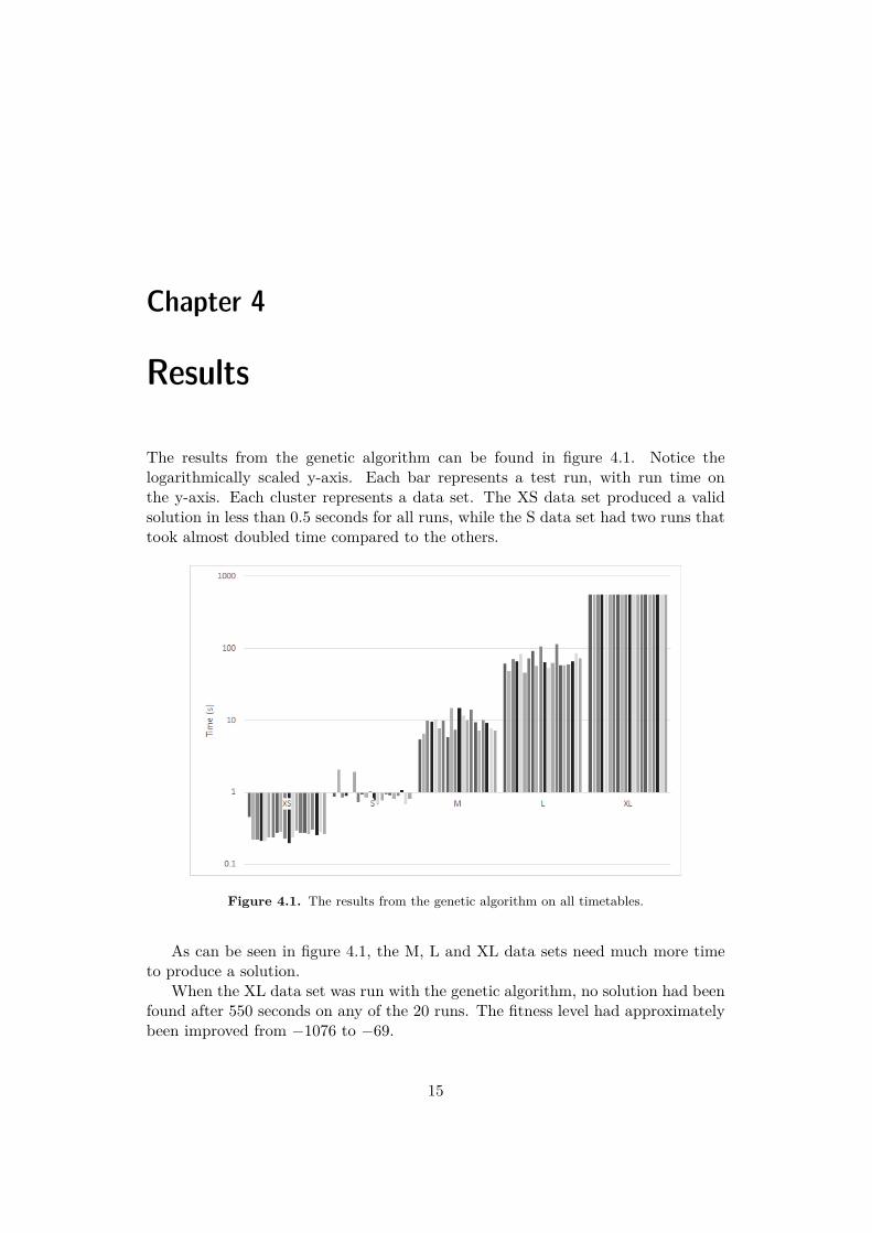
The results from the genetic algorithm can be found in figure 4.1. Notice thelogarithmically scaled y-axis. Each bar represents a test run, with run time onthe y-axis. Each cluster represents a data set. The XS data set produced a validsolution in less than 0.5 seconds for all runs, while the S data set had two runs thattook almost doubled time compared to the others.

Figure 4.1. The results from the genetic algorithm on all timetables.

As can be seen in figure 4.1, the M, L and XL data sets need much more timeto produce a solution.

When the XL data set was run with the genetic algorithm, no solution had beenfound after 550 seconds on any of the 20 runs. The fitness level had approximatelybeen improved from −1076 to −69.

15

16 CHAPTER 4. RESULTS

The simulated annealing results can be found in figure 4.2. This chart also has alogarithmically scaled y-axis, however the chart in figure 4.1 has a ten times highervalue on the y-axis. The bars and clusters still represent run time and data sets.

As can be seen in figure 4.2, the spread between runs is noticeable. However, thetime consumption is for all test runs smaller than the genetic algorithm’s respectivetest runs.

Figure 4.2. The results from the simulated annealing on all timetables.

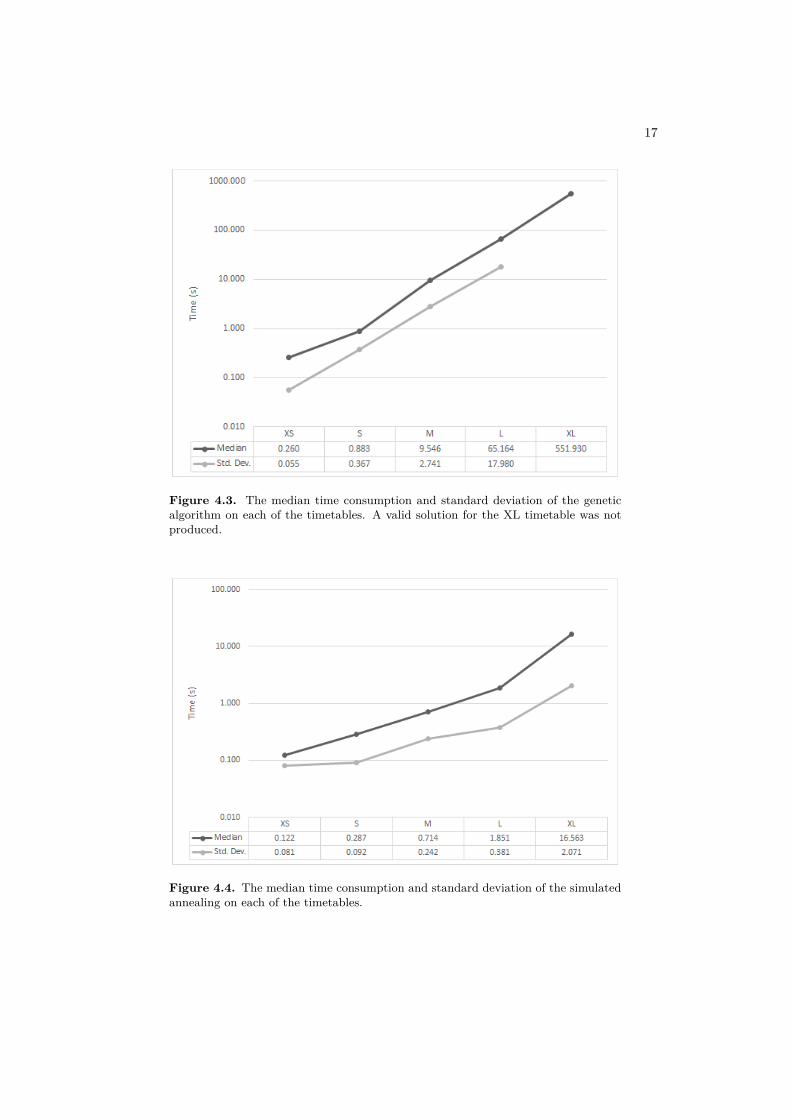
The median time consumption and the standard deviation for the differenttimetables were plotted in figure 4.3 and figure 4.4. For comparative reasons, the XLruns were plotted in the genetic algorithm chart, even though they did not producea valid solution. Both charts are drawn with a logarithmically scaled y-axis. Thegenetic algorithm overall performs worse than the simulated annealing algorithmwith respect to time consumption.

17

Figure 4.3. The median time consumption and standard deviation of the geneticalgorithm on each of the timetables. A valid solution for the XL timetable was notproduced.

Figure 4.4. The median time consumption and standard deviation of the simulatedannealing on each of the timetables.

18 CHAPTER 4. RESULTS

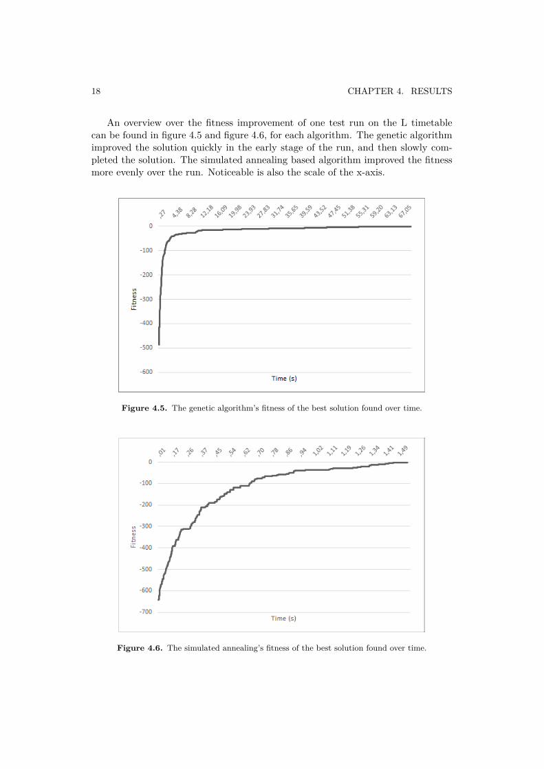
An overview over the fitness improvement of one test run on the L timetablecan be found in figure 4.5 and figure 4.6, for each algorithm. The genetic algorithmimproved the solution quickly in the early stage of the run, and then slowly com-pleted the solution. The simulated annealing based algorithm improved the fitnessmore evenly over the run. Noticeable is also the scale of the x-axis.

Figure 4.5. The genetic algorithm’s fitness of the best solution found over time.

Figure 4.6. The simulated annealing’s fitness of the best solution found over time.

19

The fitness value of the current solution for one test run on the L timetable withsimulated annealing was plotted in figure 4.7. An increasing segment indicates thata better solution was accepted, and a decreasing segment indicates that a worsesolution was accepted.

Figure 4.7. The simulated annealing’s fitness of the current solution over time.

Chapter 5

Discussion

This chapter presents an analysis of the time consumed by the algorithms, fol-lowed by the differences between them. After that, the reliability of the study iscommented, and some possible improvements are suggested.

5.1 Time complexityThe time consumed by the algorithms for solving the same problems increased morethan linear when adding events and time slots to the data set. However, the geneticalgorithm showed to grow faster when the input data increased.

What is interesting is the relatively rapid increase in fitness in the beginning ofthe genetic algorithm. The simulated annealing algorithm is however still better forevery given time interval. In their report, Pertoft and Yamazaki [13] makes a fewproposals to further improve their algorithm.

Given that these improvements would indeed result in a more optimized geneticalgorithm, a hybrid of the two algorithms could turn out to perform better than eachalone. This is due to their very different behaviors, where the genetic algorithmsperforms best in the early stages and the simulated annealing in the final stages.By integrating the two, the genetic algorithm would be used in the early stages tonarrow down the search space and the simulated annealing algorithm would be usedto find the best solution in that search space.

This hybrid will of course only work if it is possible to improve the geneticalgorithm, but due to the scope of this study the suggestions given by Pertoft andYamazaki [13] have not been implemented.

5.2 Main differences between the two algorithmsThe reason for the difference in time complexity between the two algorithms aremost probably due to their different implementations. The genetic algorithm createsa large amount of bad solutions, and crosses them with each other to finally geta good one. There is, however, no assurance that the solution will get acceptable

21

22 CHAPTER 5. DISCUSSION

fast, or even ever. This randomness is most likely the reason why there are tworuns which took twice the amount of time in the S data set in figure 4.1.

The simulated annealing on the other hand, is steering its way to the finalsolution by forcing only better solutions to be produced when it approaches theend. The partial solutions are randomized over the whole search space, which thegenetic algorithm only does in special cases.

The genetic algorithm written by Pertoft and Yamazaki [13] clearly performsworse than the simulated annealing method in these five test cases.

5.2.1 Basic local search may be sufficient

The study found the concept of these advanced meta-heuristics quite excessive.When running the simulated annealing, a random neighboring time slot is pickedand substituted. Figure 4.7 does however show that almost every substitution ofneighbors to a free time slot is improving the fitness. Therefore, a local search overthese time slots would not get stuck into too many local optima. When the eventdensity is around and below 50 %, as in these tests, these two algorithms may betoo sophisticated. The computational power needed to produce and maintain allthe instances of solutions quickly becomes unmanageable.

5.3 Reliability

The tests are not very lifelike, due to the vast number of free time slots availablewhen the problem is solved. The closest data set to the situation is the XL one,which the simulated annealing algorithm handles quite well. This shows that themost benefit is obtained when there are few possible moves that do not increasefitness, where there are many local optima.

5.4 Improvements

There are some different improvements that can be made, both to the simulatedannealing algorithm specifically and the university timetabling problem solving ingeneral, in order to make them better. These are presented in this section.

5.4.1 Refined fitness function

The fitness function presented by Pertoft and Yamazaki [13] is optimized in orderto make the genetic algorithm perform better. This makes the algorithm prioritizesome properties before others. Since the same fitness function is used for the sim-ulated annealing, these properties will also be prioritized by it. These are howeverdifferent algorithms that are working differently. Therefore, a more detailed studyof the impact of the fitness function can be done to improve the overall results.

5.4. IMPROVEMENTS 23

5.4.2 Soft constraintsIn the real world an algorithm which only returns a fair schedule would not be used.To be relevant it would also need to evaluate constraints which are not vital, butwhich should still be fulfilled if possible. These are the soft constraints as mentionedin chapter 2. To fulfill these objectives our simulated annealing algorithm wouldneed an implementation of soft constraints.

These constraints could be implemented in the two ways described in chap-ter 2.2.1: either as a one stage or a two stage algorithm. If implemented as atwo stage algorithm a hard constraint solution would first need to be found by thealgorithm. By then using a fitness function which gives positive values if a softconstraint is fulfilled, the hard constraint solution could be optimized further.

If the algorithm was going to be designed as a one stage algorithm, both of thesoft and hard constraint would need to be evaluated at the same time. To avoidgetting a solution which fulfills soft constraints but violates hard constraints, thehard constraint fitness function would have to return higher penalty values thanthe soft constraint fitness function. This would result in that a breaking of a hardconstraint would be such a high negative value that a fulfillment of several softconstraints would not nearly balance the end value. For future work, inspirationcan be taken from Bogdanov [3], who presents a solution using this method.

Chapter 6

Conclusions

The implemented simulated annealing algorithm performs much better than thegenetic algorithm by Pertoft and Yamazaki [13], with respect to time consumptionin the context of this problem. The genetic algorithm performs relatively betterthan the simulated annealing in the early stages, whereas the latter performs betterin the final stages. Increasing the event density and number of time slots resultsin a seemingly exponential time increase for both of the algorithms, which was tobe expected since the university timetabling problem in general is NP-complete.Possible future work would be to improve the genetic algorithm in accordance toPertoft and Yamazaki [13], to complement the simulated annealing thus creating amore optimized, hybrid algorithm.

25

Bibliography

[1] H. Andersson. “School Timetabling in Theory and Practice”. Bachelor’s thesis.Umeå: Umeå Universitet, 2015.

[2] Y. Awad, A. Badr, and A. Dawood. “An evolutionary immune approach foruniversity course timetabling”. In: IJCSNS International Journal of ComputerScience and Network Security 11.2 (2011), pp. 127–135.

[3] D. Bogdanov. “A Comparative Evaluation of Metaheuristic Approaches tothe Problem of Curriculum-Based Course Timetabling”. Bachelor’s thesis.Stockholm: Royal Instititue of Technology, KTH, 2015.

[4] E. Burke et al. “Automatic University Timetabling: The State of the Art”.In: The computer journal 40.9 (1997), pp. 565–571.

[5] R. Chen and H. Shih. “Solving University Course Timetabling Problems UsingConstriction Particle Swarm Optimization with Local Search”. In: Algorithms2013.6 (2013), pp. 227–244.

[6] N. Dulay. Genetic Algorithms. Visited 2016-03-27. 1999. url: http://www.doc.ic.ac.uk/~nd/surprise_96/journal/vol1/hmw/article1.html.

[7] M. Fesanghary et al. “Hybridizing harmony search algorithm with sequentialquadratic programming for engineering optimization problems”. In: Comput.Methods Appl. Mech. Engrg doi:10.1016/j.cma.2008.02.006 (2008).

[8] L. Jacobson. Simulated Annealing for Beginners. Visited 2016-03-17. 2013.url: http : / / www . theprojectspot . com / tutorial - post / simulated -annealing-algorithm-for-beginners/6.

[9] S. Kirkpatrick, C. D. Gelatt, and M. P. Vecchi. “Optimization by SimulatedAnnealing”. In: Science 220.4598 (1983), pp. 671–680.

[10] R. Lewis. “A survey of metaheuristic-based techniques for university timetablingproblems”. In: OR Spectrum 30 (2007), pp. 167–190.

[11] Z. Lü and J. Hao. “Solving the Course Timetabling Problem with a HybridHeuristic Algorithm”. In: AJMSA LNAI 5253 (2008), pp. 262–273.

[12] M. Mitchell. An Introduction to Genetic Algorithms. Cambridge, MA: MITPress, 1996. isbn: 9780585030944.

27

28 BIBLIOGRAPHY

[13] J. Pertoft and H. V. Yamazaki. “Scalability of a Genetic Algorithm that solvesa University Course Scheduling Problem Inspired by KTH”. Bachelor’s thesis.Stockholm: Royal Instititue of Technology, KTH, 2014.

[14] C. Renman and H. Fristedt. “A comparative analysis of a Tabu Search anda Genetic Algorithm for solving a University Course Timetabling Problem”.Bachelor’s thesis. Stockholm: Royal Institute of Technology, KTH, 2014.

Appendix A

Source code

The Java source code for the implemented algorithms can be found in the publicGitHub repository found at https://github.com/jonasdahl/algorithm-comparison.

29

Appendix B

Data sets

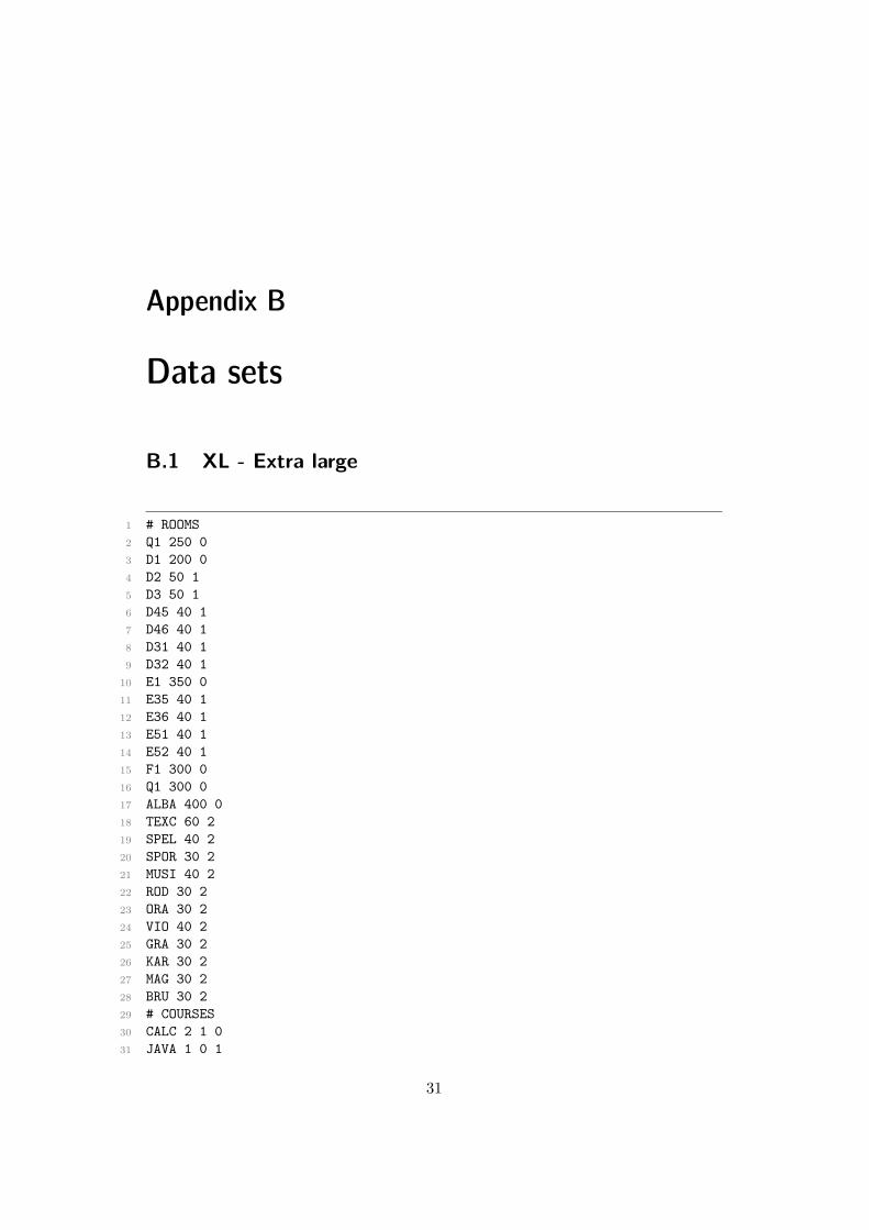
B.1 XL - Extra large

1 # ROOMS2 Q1 250 03 D1 200 04 D2 50 15 D3 50 16 D45 40 17 D46 40 18 D31 40 19 D32 40 1

10 E1 350 011 E35 40 112 E36 40 113 E51 40 114 E52 40 115 F1 300 016 Q1 300 017 ALBA 400 018 TEXC 60 219 SPEL 40 220 SPOR 30 221 MUSI 40 222 ROD 30 223 ORA 30 224 VIO 40 225 GRA 30 226 KAR 30 227 MAG 30 228 BRU 30 229 # COURSES30 CALC 2 1 031 JAVA 1 0 1

31

32 APPENDIX B. DATA SETS

32 MULT 2 0 133 CTEC 1 2 034 CSEC 0 1 135 SCON 1 1 136 DIGI 1 0 137 ENGM 1 0 138 ALGD 1 1 039 ELEC 1 0 040 PROB 1 0 141 OPER 1 1 042 TERM 2 0 143 DIFF 2 1 044 MECH 0 1 245 QUAN 1 1 046 OOPC 1 1 147 TCHE 2 1 048 PERS 1 0 049 REAC 1 0 250 POLY 1 1 051 MAGN 2 2 052 POLT 3 2 153 NUMD 2 2 354 TERT 2 0 055 DDED 3 2 056 MAGA 3 1 057 NUMA 3 1 358 TERA 3 1 059 # LECTURERS60 SVEN CALC MULT61 BERT JAVA SCON OOPC62 KARL CSEC63 GUNN CTEC64 BERI DIGI65 ERIK DIFF POLT66 SARA OPER67 OLLE ENGM ELEC68 BENG ALGD69 JUDI TERM REAC70 MANS MECH MAGN71 MICH QUAN72 PELL PROB73 DARI TCHE POLY74 MORT PERS75 LEFT TERA76 PATR TERT77 MIHA DDED78 DILI NUMA79 CGRI NUMD80 STEF MAGA

B.2. L - LARGE 33

81 # STUDENTGROUPS82 COMP_1 200 CALC JAVA83 COMP_2 120 MULT CTEC84 COMP_3 70 CSEC SCON85 INFO_1 200 DIGI ENGM86 INFO_2 100 ALGD ELEC87 INFO_3 50 PROB OPER88 PHYS_1 200 CALC TERM89 PHYS_2 180 DIFF MECH90 PHYS_3 100 QUAN OOPC91 CHEM_1 150 CALC TCHE92 CHEM_2 130 PERS DIFF93 CHEM_3 100 REAC MAGN94 DDOS_1 150 POLY POLT95 DDOS_2 140 NUMD TERT96 DDOS_3 120 MAGA DDED97 BIZZ_1 150 POLY POLT98 BIZZ_2 140 TERA99 BIZZ_3 120 NUMA

100 MIZZ_1 50 POLY MECH101 MIZZ_2 40 CALC102 MIZZ_3 20 ELEC

B.2 L - Large

1 # ROOMS2 D1 200 03 D2 50 14 D3 50 15 D45 40 16 D46 40 17 E1 350 08 E35 40 19 E36 40 1

10 F1 300 011 SPEL 40 212 SPOR 30 213 MUSI 40 214 ROD 30 215 ORA 30 216 VIO 40 217 GRA 30 218 # COURSES19 CALC 2 1 020 JAVA 1 0 121 MULT 2 0 122 CTEC 1 2 0

34 APPENDIX B. DATA SETS

23 CSEC 0 1 124 SCON 1 1 125 DIGI 1 0 126 ENGM 1 0 127 ALGD 1 1 028 ELEC 1 0 029 PROB 1 0 130 OPER 1 1 031 TERM 2 0 132 DIFF 2 1 033 MECH 0 1 234 QUAN 1 1 035 OOPC 1 1 136 TCHE 2 1 037 PERS 1 0 038 REAC 1 0 239 POLY 1 1 040 # LECTURERS41 SVEN CALC MULT42 BERT JAVA SCON OOPC43 KARL CSEC44 GUNN CTEC45 BERI DIGI46 ERIK DIFF47 SARA OPER48 OLLE ENGM ELEC49 BENG ALGD50 JUDI TERM REAC51 MANS MECH52 MICH QUAN53 PELL PROB54 DARI TCHE POLY55 MORT PERS56 # STUDENTGROUPS57 COMP_1 200 CALC JAVA58 COMP_2 120 MULT CTEC59 COMP_3 70 CSEC SCON60 INFO_1 200 DIGI ENGM61 INFO_2 100 ALGD ELEC62 INFO_3 50 PROB OPER63 PHYS_1 200 CALC TERM64 PHYS_2 180 DIFF MECH65 PHYS_3 100 QUAN OOPC66 CHEM_1 150 CALC TCHE67 CHEM_2 130 PERS DIFF68 CHEM_3 100 REAC POLY

B.3. M - MEDIUM 35

B.3 M - Medium

1 # ROOMS2 D1 200 03 D2 50 14 D3 50 15 D45 40 16 D46 40 17 E1 350 08 E35 40 19 SPEL 40 2

10 SPOR 30 211 MUSI 40 212 ROD 30 213 ORA 30 214 # COURSES15 CALC 2 1 016 JAVA 1 0 117 MULT 2 0 118 CTEC 1 2 019 CSEC 0 1 120 SCON 1 1 121 DIGI 1 0 122 ENGM 1 0 123 ALGD 1 1 024 ELEC 1 0 025 PROB 1 0 126 OPER 1 1 027 TERM 2 0 128 DIFF 2 1 029 MECH 0 1 230 QUAN 1 1 031 OOPC 1 1 132 TCHE 2 1 033 PERS 1 0 034 REAC 1 0 235 POLY 1 1 036 # LECTURERS37 SVEN CALC MULT38 BERT JAVA SCON OOPC39 KARL CSEC40 GUNN CTEC41 BERI DIGI42 ERIK DIFF43 SARA OPER44 OLLE ENGM ELEC45 BENG ALGD46 JUDI TERM REAC

36 APPENDIX B. DATA SETS

47 MANS MECH48 MICH QUAN49 PELL PROB50 DARI TCHE POLY51 MORT PERS52 # STUDENTGROUPS53 COMP_1 200 CALC JAVA54 COMP_2 120 MULT CTEC55 COMP_3 70 CSEC SCON56 INFO_1 200 DIGI ENGM57 INFO_2 100 ALGD ELEC58 INFO_3 50 PROB OPER59 PHYS_1 200 CALC TERM60 PHYS_2 180 DIFF MECH

B.4 S - Small

1 # ROOMS2 D1 200 03 D3 50 14 D45 40 15 E1 350 06 E35 40 17 SPEL 40 28 SPOR 30 29 MUSI 40 2

10 # COURSES11 CALC 2 1 012 JAVA 1 0 113 MULT 2 0 114 CTEC 1 2 015 CSEC 0 1 116 SCON 1 1 117 DIGI 1 0 118 ENGM 1 0 119 ALGD 1 1 020 ELEC 1 0 021 PROB 1 0 122 OPER 1 1 023 TERM 2 0 124 DIFF 2 1 025 MECH 0 1 226 QUAN 1 1 027 OOPC 1 1 128 TCHE 2 1 029 PERS 1 0 030 REAC 1 0 2

B.5. XS - EXTRA SMALL 37

31 POLY 1 1 032 # LECTURERS33 SVEN CALC MULT34 BERT JAVA SCON OOPC35 KARL CSEC36 GUNN CTEC37 BERI DIGI38 ERIK DIFF39 SARA OPER40 OLLE ENGM ELEC41 BENG ALGD42 JUDI TERM REAC43 MANS MECH44 MICH QUAN45 PELL PROB46 DARI TCHE POLY47 MORT PERS48 # STUDENTGROUPS49 COMP_1 200 CALC JAVA50 COMP_2 120 MULT CTEC51 COMP_3 70 CSEC SCON52 INFO_1 200 DIGI ENGM53 INFO_2 100 ALGD ELEC54 INFO_3 50 PROB OPER

B.5 XS - Extra small

1 # ROOMS2 D1 200 03 D45 40 14 E35 40 15 SPEL 40 26 SPOR 30 27 # COURSES8 CALC 2 1 09 JAVA 1 0 1

10 MULT 2 0 111 CTEC 1 2 012 CSEC 0 1 113 SCON 1 1 114 DIGI 1 0 115 ENGM 1 0 116 ALGD 1 1 017 ELEC 1 0 018 PROB 1 0 119 OPER 1 1 020 TERM 2 0 1

38 APPENDIX B. DATA SETS

21 DIFF 2 1 022 MECH 0 1 223 QUAN 1 1 024 OOPC 1 1 125 TCHE 2 1 026 PERS 1 0 027 REAC 1 0 228 POLY 1 1 029 # LECTURERS30 SVEN CALC MULT31 BERT JAVA SCON OOPC32 KARL CSEC33 GUNN CTEC34 BERI DIGI35 ERIK DIFF36 SARA OPER37 OLLE ENGM ELEC38 BENG ALGD39 JUDI TERM REAC40 MANS MECH41 MICH QUAN42 PELL PROB43 DARI TCHE POLY44 MORT PERS45 # STUDENTGROUPS46 COMP_1 200 CALC JAVA47 COMP_2 120 MULT CTEC48 COMP_3 70 CSEC SCON

www.kth.se