a comparative study of simulated annealing and self

IN DEGREE PROJECT ELECTRONICS AND COMPUTER ENGINEERING,FIRST CYCLE, 15 CREDITS

, STOCKHOLM SWEDEN 2020

A Comparative Study of Simulated Annealing and Self-Organising Map Batching for Solving the Order Batching Problem in Warehouses

FRANS TEGELMARK

NILS STREIJFFERT

KTH ROYAL INSTITUTE OF TECHNOLOGYSCHOOL OF ELECTRICAL ENGINEERING AND COMPUTER SCIENCE

A Comparative Study ofSimulated Annealing andSelf-Organising Map Batchingfor Solving the OrderBatching Problem inWarehouses

FRANS TEGELMARK & NILS STREIJFFERT

Degree Project in Computer Science, DD142XDate: June 8, 2020Supervisor: Jörg ConradtExaminer: Pawel HermanSchool of Electrical Engineering and Computer ScienceSwedish title: En jämförande studie mellan self-organising mapbatching och simulated annealing för att lösa order batchingproblemet för lager

iii

AbstractWarehouses need e�cient picking strategies. Batching orders is one such strat-egy, but creating e�cient batches out of orders is computationally hard. Wecompare two algorithms to find approximate solutions to the batching prob-lem; the general global optimisation algorithm Simulated Annealing and thebatching specific algorithm Self-Organising Map Batching (SOMB).

The results demonstrate that for a small number of orders, Simulated An-nealing performs better than SOMB, but takes longer to run. For a large num-ber of orders, SOMB performs better than Simulated Annealing and generatesthe result quicker. Which algorithm is the best at batching orders depends onthe number of orders that are being batched.

iv

SammanfattningLager behöver e�ektiva orderplocks-stragier. Att gruppera ordrar i större set ären strategi, men att skapa e�ekiva ordergrupper är beräkningsintensivt. I dethär arbetet jämför vi två algoritmer som ger approximativa lösningar på proble-met; den generella globala optimeringsalgoritmen Simulated Annealing (sv.simulerad avsvalning) och den ordergrupperings-specifika algoritmen Self-Organising Map Batching (SOMB).

Resultatet visar att för en liten mängd ordrar så genererar Simulated Anne-aling bättre lönsingar än SOMB, men kräver en längre beräkningstid. För sto-ra mängder ordrar så generar SOMB bättre lösningar än Simulated Annealingoch har en kortare beräkningstid. Vilken algoritm som är bäst på att grupperaordrar beror därmed på antalet ordrar som ska grupperas.

Contents

1 Introduction 21.1 Purpose . . . . . . . . . . . . . . . . . . . . . . . . . . . . . 31.2 Problem Statement . . . . . . . . . . . . . . . . . . . . . . . 31.3 Delimitations and Scope . . . . . . . . . . . . . . . . . . . . 3

2 Background 42.1 The Travelling Salesperson Problem . . . . . . . . . . . . . . 42.2 The Order Batching Problem . . . . . . . . . . . . . . . . . . 42.3 Self-Organising Map . . . . . . . . . . . . . . . . . . . . . . 52.4 Self-Organising Map Batching . . . . . . . . . . . . . . . . . 52.5 Simulated Annealing . . . . . . . . . . . . . . . . . . . . . . 62.6 2-Opt . . . . . . . . . . . . . . . . . . . . . . . . . . . . . . 72.7 Related Work . . . . . . . . . . . . . . . . . . . . . . . . . . 7

3 Method 93.1 Experiments . . . . . . . . . . . . . . . . . . . . . . . . . . . 93.2 Evaluation . . . . . . . . . . . . . . . . . . . . . . . . . . . . 103.3 Experiment Setup . . . . . . . . . . . . . . . . . . . . . . . . 10

3.3.1 Test Data . . . . . . . . . . . . . . . . . . . . . . . . 103.3.2 Warehouses . . . . . . . . . . . . . . . . . . . . . . . 103.3.3 Environment . . . . . . . . . . . . . . . . . . . . . . 13

3.4 Self-Organising Map Batching . . . . . . . . . . . . . . . . . 133.5 Simulated Annealing . . . . . . . . . . . . . . . . . . . . . . 14

3.5.1 Initial State . . . . . . . . . . . . . . . . . . . . . . . 143.5.2 Generating Neighbour States . . . . . . . . . . . . . . 143.5.3 Calculating the Energy of a State . . . . . . . . . . . . 153.5.4 Cooling Schedule . . . . . . . . . . . . . . . . . . . . 15

4 Results 16

v

CONTENTS 1

5 Discussion 295.1 The Running Time of the Algorithms . . . . . . . . . . . . . . 295.2 Hyperparameters . . . . . . . . . . . . . . . . . . . . . . . . 305.3 Further Research . . . . . . . . . . . . . . . . . . . . . . . . 30

6 Conclusions 32

Bibliography 33

A Warehouses 35A.1 Warehouse 1 . . . . . . . . . . . . . . . . . . . . . . . . . . . 35A.2 Warehouse 2 . . . . . . . . . . . . . . . . . . . . . . . . . . . 36A.3 Warehouse 3 . . . . . . . . . . . . . . . . . . . . . . . . . . . 37

B Simulated Annealing Schedules 38

C Graphs 40

Chapter 1

Introduction

Warehouses have always played a crucial role in the supply chain, yet with thegrowth of e-commerce, their importance has increased. They are no longerjust a place for storage of goods; they are centres for value-creation Today’swarehouses often have assembly and packaging centres to fulfil customers or-ders directly on the premise [1].

Warehouse layout, how products are stored and grouped, the way workersare organised and move around the facility are all aspects of warehouse opera-tions that can be optimised [2]. Hsieh and Huang [3] found that order pickingaccounts for over 55 percent of overall operating cost for warehouses. The or-der picking problem can be broken down into three sub-problems: an item’sstorage location, order batching and picker routing problem [4]. This thesisis concerned with optimising order batching, which is a well researched NP-hard problem. That the problem is NP-hard means that the problems cannotbe solved in polynomial time (under the assumption that P 6= NP )

Solving the Order Batching Problem means finding the most e�cient wayof putting orders or parts of orders together forming a so-called batch [4].

One approach to solving the batching problem is using the probabilisticapproximating algorithm Simulated Annealing (SA). It has been found to saveover 5 000 km in travel distance for order pickers in real-world warehousesover three months in comparison with the previously used routing strategy[5]. Another approach to solving the batching problem is Self-Organising MapBatching (SOMB), it uses an Artificial Neural Network (ANN) to cluster sim-ilar orders with the hope that this reduces the total travel distance for orderpickers.

2

CHAPTER 1. INTRODUCTION 3

1.1 PurposeSince order picking constitutes a large percentage of the operating cost of awarehouse, it must be done as e�ciently as possible. Self-organising-mapbatching is a relatively new approach to solving the batching problem. We,therefore, want to compare it to Simulated Annealing, which is a more tradi-tional approach to solving the batching problem. The objective of the thesisis, therefore, to determine which algorithm is better at solving the batchingproblem in warehouses.

1.2 Problem StatementWhich algorithm is best at minimising the total travel distance for the ware-

house Order Batching Problem out of Simulated Annealing and Self Organis-

ing Map Batching?

1.3 Delimitations and ScopeThe objective of this thesis is to compare two specific implementations of Sim-ulated Annealing and Self-Organising Map Batching, not to compare the al-gorithms in general.

For this thesis, the carrying capacity of an order picker is defined as thebatch volume limit. We assume that all warehouses have a rectangle shape andthat they are divided into cells. The cells can either be paths, shelves or walls.All tours in the warehouse start and end at the same cell, henceforth known asthe drop o� point. All path cells are reachable from the drop o� point. Thedistances in the warehouse are measured in the number of traversed nodes. Allorders are known in advance as well as the shortest path between each pathcell. The distance of a batch is approximated using the local search algorithm2-Opt.

Chapter 2

Background

This chapter provides an overview of the Travelling Salesperson Problem, theOrder Batching Problem, Self-Organising Maps, Self-Organising Map Batch-ing, Simulated Annealing and 2-Opt. The chapter also includes an overviewof related works.

2.1 The Travelling Salesperson ProblemThe Travelling Salesperson Problem (TSP) is defined as given a set of cities{c1, c2, ..., cN} and for each pair {ci, cj} of distinct cities a distance d(ci, cj).Find an order ⇡ of the cities that minimises the quantity also called tour length

given by Equation 2.1 [6]. The Travelling Salesperson Problem is NP-hard[6].

N�1X

i=1

d(c⇡(i), c⇡(i+1))) + d(c⇡(N), c⇡(1)) (2.1)

2.2 The Order Batching ProblemThe purpose of a warehouse is to store items until they are needed. Whenan item is requested, the retrieval process must be as e�cient as possible. Acommon way of structuring order retrieval in warehouses is that set of ordersare split into several subsets, called batches. Batches are then assigned topickers who each retrieve all the items in a single batch at a time and then dropo� all the items at the drop of point where they are later packed and shipped.

4

CHAPTER 2. BACKGROUND 5

Since up to 55 percent of the operating cost of a warehouse comes from itemretrieval [3] it is crucial to find the most e�cient way to group orders.

To avoid having the pickers go back to the drop o� point too often, thebatches should all be as large as possible within the capacity limits of thepickers. It is this problem that the Order Batching Problem aims to solve,which combination of orders results in the shortest total travel distance for theitem picking agents. The batching problem is computationally expensive andis solved using approximation methods.

For every batch, there exists a minimum distance that an agent needs totravel to retrieve it. Finding this distance is an NP-hard problem since it meanssolving TSP. This step is not necessary for all batching algorithms to gener-ate their solution. However, it is required to evaluate the performance of theoutput.

2.3 Self-Organising MapSelf-Organising Map (SOM) is a technique that uses an artificial neural net-work (ANN) that is trained using unsupervised learning to reduce the dimen-sion of a data set. The technique was developed by the Finish professor TeuvoKohonen in 1982 [7].

The idea behind the technique is to simulate how the brain is structured,where cells with similar functionality group together, for example, cells relatedto taste and sight. When the brain receives di�erent stimuli, di�erent areasof the cortex reacts, and a topological mapping is formed through the neuralsystem learning process. This training, when completed, makes the neuralsystem capable of correctly reflecting the received stimulation [8]. It is theformation of this mapping through the neural system’s learning process thatenables SOM to reduce the dimensionality of the input data.

2.4 Self-Organising Map BatchingThe Self-Organising Map Batching (SOMB) algorithms groups similar orderstogether into clusters using a SOM [8]. The SOM is trained on orders from thesame distribution as those that will later be batched. The batches are createdone by one by taking the biggest yet unbatched order and then placing otherorders that are similar to it on the SOM in the same batch until the volumelimit of pickers is reached. At that point, the next batch is started, and theprocess continues until all orders are in a batch. With a fixed trained SOM

6 CHAPTER 2. BACKGROUND

this algorithm is deterministic.This process is greedy and only guided by the SOM as heuristic. This

makes it fast and it can proceed without the complication or cost of evaluatingthe quality of the batches. These upsides are also the downsides. The greedyapproach means it doesn’t reconsider alternative solutions and without any wayto evaluate batches it isn’t really possible to modify it to do so. Similarity be-tween orders is loosely the amount of items that are close to some items in theother order. Items that are close to paths that will be travelled between itemsthat are in a batch are thus not considered similar. These paths are computedafter the SOMB algorithm completes which makes them unavailable for thealgorithm.

2.5 Simulated AnnealingSimulated Annealing (SA) is a probabilistic algorithm for finding the optimalglobal solution for a function. The algorithm derives its name the process ofslowly cooling a physical system in order to obtain states with globally mini-mum energy [9]. Simulated Annealing is a heuristic which means that it is notguaranteed to find the optimal global solution.

The algorithm starts with an initial temperature and a random state. Af-ter the initial setup, the algorithm starts its main loop where it first choosesa neighbour state of the current state and calculates the energy of the neigh-bour. Then the algorithm decides if it should swap the current state with theneighbour state. The decision is based on the di�erence in energy between thetwo states and the current temperature. If the energy of the neighbour state islower then the current state, the neighbour state is set as the current state. Ifthe energy of the neighbour state is higher than the current state, the decisionto keep the neighbour state is decided by a temperature-dependent probabilityfunction. The higher the current temperature is, the higher the chance that astate with a higher temperature is kept. After the decision has been made, thesystem temperature is decreased, and the loop restarts. The loop repeats untila predetermined final temperature has been reached.

CHAPTER 2. BACKGROUND 7

2.6 2-OptThe 2-opt algorithm is a local search algorithm for TSP, that was originallyproposed in 1958 by Croes [10]. However, the primary move of the algorithmhad already been suggested two years earlier in 1956 by Flood [11]. The al-gorithm aims to remove any instances of the tour crossing over itself. Thealgorithm works by deleting two edges in the tour and reconnecting the nodes.A visualisation of the 2-Opt algorithm being applied to a TSP tour can befound in Figure 2.1.

Figure 2.1: A 2-Opt move: original tour on the left and resulting tour on theright [6].

2.7 Related WorkIn an article by Matusiak et al. [5] from 2013, the authors proposed a joint orderbatching and picker routing method to solve the combined routing and order-batching problem. They used the A*-algorithm to solve the routing problemand Simulated Annealing to solve the batching problem. The approach wastested on sets of three orders and was found to be only 1.2 percent worse thanthe optimal solution.

In their thesis from 2019 Ardö and Lindholm [12] compared two meta-heuristics Simulated Annealing and a Genetic algorithm for solving the order-batching problem. They found that Simulated Annealing performed better orequally as good as the Genetic algorithm at minimising the total travel distance.

8 CHAPTER 2. BACKGROUND

They also found that Simulated Annealing finds the shortest solution fasterthan the Genetic algorithm.

Theys et al. [13] compared the Lin–Kernighan–Helsgaun (LKH) TSP heuris-tic with existing dedicated order picker heuristics and found an average savingin route distance of up to 47 percent when using LKH.

De Koster and Van Der Poort [14] compared optimal and heuristic solu-tions for routing pickers in warehouses. They found that the optimal solutionreduced the travel time per route between 7 and 34 percent compared with theheuristic. However, they also found that the reduction in time strongly dependson the layout and operation of the warehouse.

Su [15] designed an automated control mechanism for the planning of or-der picking by combining a neural network with Simulated Annealing. Al-though the author of the paper did not fully test the performance of the system,the limited test that where performed showed promising results.

Chapter 3

Method

This chapter describes the experiments performed to answer the research ques-tion. The chapter also contains information about the test setup, how the testdata was generated and implementation details for both Simulated Annealingand Self-Organising Map Batching.

3.1 ExperimentsTwelve experiments were designed to help answer the research question, seeTable 3.1 for an overview of the experiments. Each experiment was run 15times per warehouse for Simulated Annealing and once for SOMB. The rea-son for running Simulated Annealing multiple times for each experiment andSOMB once is that Simulated Annealing is non-deterministic while SOMB isdeterministic.

Experiment Number of orders Max items per order Item volume limit Batch volume limit1 10 5 20 1322 10 10 20 2413 10 15 20 3504 10 20 20 4585 100 5 20 1326 100 10 20 2417 100 15 20 3508 100 20 20 4589 500 5 20 13210 500 10 20 24111 500 15 20 35012 500 20 20 458

Table 3.1: An overview of the experiments.

9

10 CHAPTER 3. METHOD

The batch volume limit depends on the maximum number of items allowedin an order and is four times the average order volume. The reason for pickingthis volume limit is that we want to test the capability of the algorithm to batchorders. If the volume limit is too small, the algorithms would not be able tofind any orders to combine into batches. If the order limit is too big, then thealgorithms could combine all the orders into one or two batches.

3.2 EvaluationThe resulting batches from each algorithm are compared by calculating thetotal tour distance for each set of batches. Since calculating the tour distancefor a batch means solving TSP, we can not calculate the exact distance foreach batch. We instead approximate the tour distance using the local searchalgorithm 2-Opt. The algorithm is run for 30 seconds for each set of batchesto produces a comparable result.

3.3 Experiment SetupThis section provides an overview of the warehouses and the test environment.

3.3.1 Test DataThe warehouse shelves are filled with items, and then orders are generated witha weighted distribution where shelves that are closer to the drop o� point willbe accessed more often. We chose to make a distribution where 80 percentof the item types that are ordered are selected from the 20 percent items onthe closest shelves. The reason for choosing this distribution is to simulate awarehouse sorted with high throughput items closer to the drop o� point. Sincewe are using a SOM, which organises structure in data, order data generatedwith a uniform distribution and no structure is unlikely to produce good results.

3.3.2 WarehousesA warehouse is a rectangle, divided into cells that can be either paths, shelvesor walls. Each warehouse has one drop o� point where the agent that picks theitems in the orders begin and end their trip. The warehouses are stored in textfiles, where the first two lines are integers representing the warehouse widthand height. The following lines are the warehouse layout placed inside a square

CHAPTER 3. METHOD 11

of number signs (#). Paths are encoded as spaces; shelves can be encoded withfour di�erent characters (see table 3.2) depending on from which side the shelfis accessible. Walls can be any character not used to encode paths or shelvesor X, which is used to mark the drop-o� point in the warehouse. The drop-o�point is also a path that the agent can traverse.

Character Access direction Access coordinates] From the cell to the left (x� 1, y)[ From the cell to the right (x+ 1, y)v From the cell above (x, y + 1)^ From the cell below (x, y � 1)

Table 3.2: Characters used to encode shelves in the text representation of thewarehouse.

The warehouses are converted into graphs using the NetworkX Python li-brary [16]. The graph representations of the warehouses allow us to calculatethe shortest distance between all the items using NetworkX’s implementationof the A* algorithm. The calculated distances are stored in a distance matrix.This allows us to have an instant lookup time for the shortest path betweenitems in the warehouse. We also calculate the shortest distance between allthe items and the drop o� point.

Three warehouses were designed for this thesis. Warehouse one and threehas a traditional warehouse layout with long rows and few crossing aisles, andtheir layout is based on the Traditional Layout 2 from the article An Overview

of Warehouse Optimization [17]. Warehouse number two is based on theFlying-V Layout from the same article. Graph representations of the ware-houses can be seen in Figures 3.1-3.3. The text file representation of the ware-houses can be found in appendix A. For more information about the warehouselayouts, see Table 3.3.


Figure 3.1: Warehouse 1. The blue circles are path nodes, the black squaresare shelves and the red node is the drop o� point. An agent can move betweentwo path nodes if there is an edge between them.

Figure 3.2: Warehouse 2: the Flying-V warehouse layout. The blue circles arepath nodes, the black squares are shelves and the red node is the drop o� point.An agent can move between two path nodes if there is an edge between them.


Figure 3.3: Warehouse 3. The blue circles are path nodes, the black squaresare shelves and the red node is the drop o� point. An agent can move betweentwo path nodes if there is an edge between them.

Warehouse Dimensions Types of items1 13⇥ 9 562 85⇥ 30 15123 31⇥ 30 530

Table 3.3: Overview of warehouse layout.

3.3.3 EnvironmentAll test were performed on an Amazon Web Service (AWS) Amazon Elas-tic Compute Cloud (EC2) instance of type c5.4xlarge [18]. The instance isequipped with an Intel Xeon Platinum 8124M CPU (3.00GHz), 16 vCPU (16threads) and 32GB of RAM. The experiments were run in parallel, one exper-iment per thread.

3.4 Self-Organising Map BatchingOur implementation of SOMB for this thesis is written in Python. The SOM’sneural network is trained using a matrix where the rows correspond to order


IDs and the columns represents if an item ID exits in that order. If a cell iszero, it means that the item is not part of that order, if it is one the item is partof the order.

Items that are on shelves that are close to items that are part of orders thathave been batched do not require us to extend our picking tour if they areincluded in a batch. The order picker would have to pass by these shelves tocomplete orders that are currently in the batch.

Items that are nearby are given a score between zero and one in the trainingmatrix. The score is calculated by the formula 1 � M/D where M is themaximum distance that is considered "close" and D is the distance we have towalk to reach this item ID from the closest position we will have to go to pickan item that is in the order. Thus items that are close in warehouse space willbe considered similar items when batching the orders.

3.5 Simulated AnnealingThe Simulated Annealing algorithm was implemented using the Python li-brary simanneal (version 0.5.0) written by Matthew Perry [19]. The libraryexposes two functions move which creates neighbour states and energy, whichcalculates the energy of a state.

3.5.1 Initial StateThe initial state is generated by placing each order into an empty batch. Thereason for placing one order per batch is to make it as easy as possible togenerate neighbour states.

3.5.2 Generating Neighbour StatesThe generate neighbour function contains two functions that are called with acertain probability. The first function picks a random order and tries to put itinto a random batch or a place it into an empty batch. The chance that an orderis placed in an empty batch is one divided by the number of batches. The orderis also placed into an empty batch if it does not fit inside any of the currentbatches. The second function tries to switch two orders from di�erent batches.The second function is called 90 percent of the time. The ratio between thefunctions was set after running several tests.

The reason that the second function is called more often than the first oneis that after a while, it becomes harder to find a batch that has space to fit a


random order and placing single order in a batch is always less e�cient.

3.5.3 Calculating the Energy of a StateThe energy of a state is defined as the total distance a picking agent wouldhave to travel to complete the batches in the state. Since finding the shortesttravel distance for each batch means solving TSP this is an NP-hard problem.We, therefore, approximate the travel distance for each batch using the localsearch algorithm 2-Opt. The algorithm is run once for each combination ofnodes in the tour. This approximation will not find the shortest path for a batch;however, it is su�cient to approximate the energy of a state.

3.5.4 Cooling ScheduleThe cooling schedules used in the experiments were found by first by usingthe simanneal library’s built-in schedule finder and then manually tuning theparameters with a few tests. The goal of the tuning was to find a schedule foreach experiment that produced good results and took on average 30 secondsto run. A complete list of cooling schedules can be found in Appendix B.

Chapter 4

Results

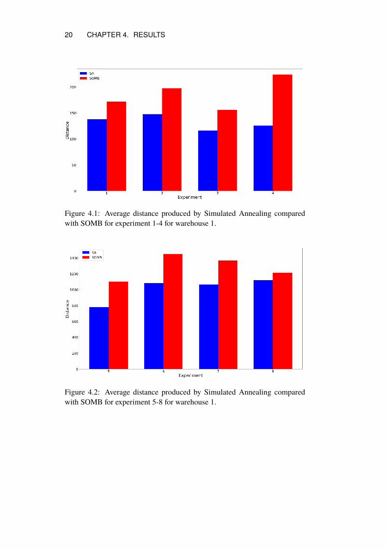
Table 4.1 shows the results for the 12 experiments for each warehouse. Simu-lated Annealing performs better than SOMB for smaller order sizes, but SOMBperforms better than SA for larger order sizes.

Figures 4.1-4.9 compares the average distance produced by Simulated An-nealing over 15 test runs with SOMB, for the three di�erent warehouses.

Tables 4.2 - 4.4 shows the variance in the distances produced by SimulatedAnnealing over 15 test runs. The distance for the batches produced by Simu-lated Annealing has a small spread, and for some of the smaller order sizes,all runs converged to the same final distance. The derivation of the resultsgenerally increased with the order size.

Table 4.5 shows the time it took for SOMB to generate a batch for eachexperiment. The results show that the duration increases with the number oforders that are being batched.

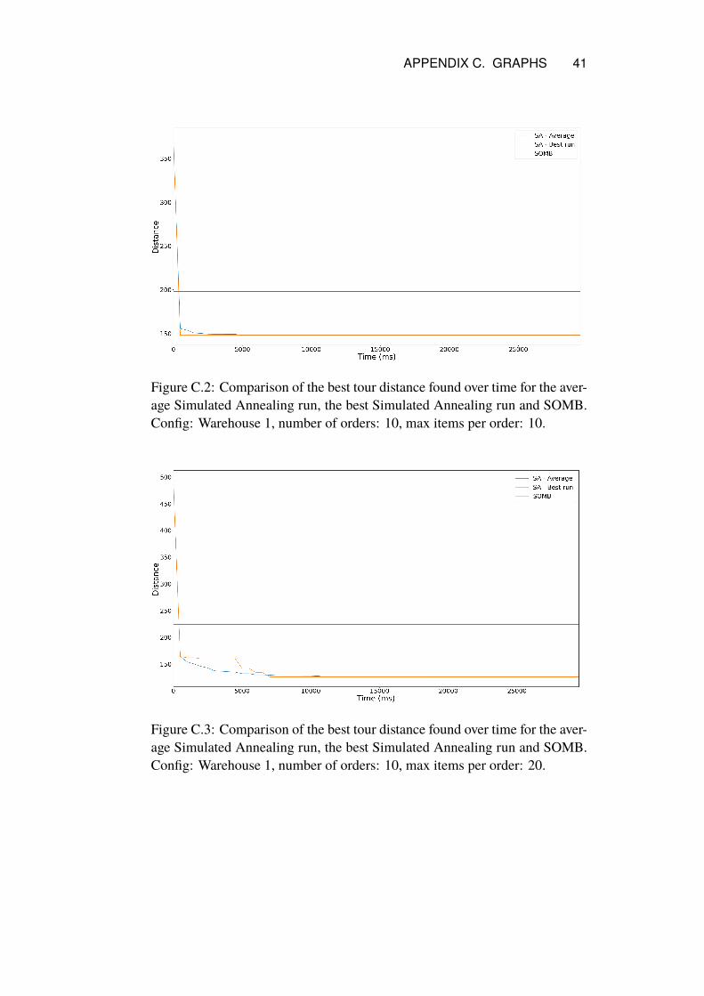
Figures 4.10-4.18 compare the best tour distances found over time for theaverage Simulated Annealing run, the best Simulated Annealing run and SOMBfor a selected number of experiments. See the complete set of graphs in Ap-pendix C.

16

CHAPTER 4. RESULTS 17

Experiment Algorithm Warehouse 1 Warehouse 2 Warehouse 31 SA 138 782 282

SOMB 172 962 3162 SA 148 1 048 429

SOMB 198 1 298 5523 SA 116 1 002 638

SOMB 156 1 166 6884 SA 126 1 588 732

SOMB 224 1 906 8945 SA 782 5 743 2 943

SOMB 1 102 7 366 3 8546 SA 1 081 8 966 4 527

SOMB 1 450 9 862 5 3807 SA 1 067 11 344 6 322

SOMB 1 370 11 174 6 0668 SA 1 118 14 813 8 166

SOMB 1 214 13 242 6 8909 SA 7 931 42 060 27 325

SOMB 5 816 34 246 20 28210 SA 12 588 72 396 43 532

SOMB 6 224 46 844 26 35211 SA 16 016 93 615 55 948

SOMB 6 628 53 978 29 63412 SA 19 629 111 237 67 550

SOMB 7 018 61 534 32 304

Table 4.1: Comparison of the average distance produced by Simulated An-nealing over 15 runs, with the result from SOMB.

18 CHAPTER 4. RESULTS

Experiment Median 1st Quartile 2nd Quartile Min Max1 138 138 138 138 1382 148 148 148 148 1483 116 116 116 116 1164 126 126 126 126 1265 782 776 788 762 8026 1 080 1 059 1 097 1 052 1 1227 1 054 1 047 1 093 1 022 1 1228 1 098 1 063 1 170 966 1 2669 7 974 7 869 8 009 7 526 8 15210 12 478 12 363 12 728 12 132 13 34411 16 018 15 898 16 257 15 550 16 29812 19 678 19 367 19 813 19 112 20 220

Table 4.2: Variance in Simulated Annealing result for warehouse 1 over 15runs.

Experiment Median 1st Quartile 2nd Quratile Min Max1 782 782 782 782 7822 1 048 1 480 1 480 1 480 1 4803 1 002 1 002 1 002 1 002 1 0024 1 586 1 586 1 586 1 586 1 6145 5 758 5 729 5 763 5 678 5 8246 8 968 8 871 9 024 8 680 9 4027 11 138 11 190 11 452 1 0804 12 2388 14 952 14 678 15 087 1 3684 15 5929 42 282 41 353 42 515 40 624 43 34010 72 400 72 042 72 928 70 808 73 76211 93 826 93 429 94 114 90 358 94 71612 111 237 110 682 111 823 109 654 112 492



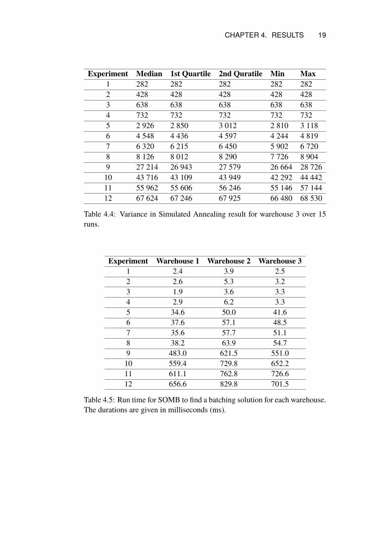
Experiment Median 1st Quartile 2nd Quratile Min Max1 282 282 282 282 2822 428 428 428 428 4283 638 638 638 638 6384 732 732 732 732 7325 2 926 2 850 3 012 2 810 3 1186 4 548 4 436 4 597 4 244 4 8197 6 320 6 215 6 450 5 902 6 7208 8 126 8 012 8 290 7 726 8 9049 27 214 26 943 27 579 26 664 28 72610 43 716 43 109 43 949 42 292 44 44211 55 962 55 606 56 246 55 146 57 14412 67 624 67 246 67 925 66 480 68 530


Experiment Warehouse 1 Warehouse 2 Warehouse 31 2.4 3.9 2.52 2.6 5.3 3.23 1.9 3.6 3.34 2.9 6.2 3.35 34.6 50.0 41.66 37.6 57.1 48.57 35.6 57.7 51.18 38.2 63.9 54.79 483.0 621.5 551.010 559.4 729.8 652.211 611.1 762.8 726.612 656.6 829.8 701.5

Table 4.5: Run time for SOMB to find a batching solution for each warehouse.The durations are given in milliseconds (ms).


Figure 4.1: Average distance produced by Simulated Annealing comparedwith SOMB for experiment 1-4 for warehouse 1.




Figure 4.10: Comparison of the best tour distance found over time for the aver-age Simulated Annealing run, the best Simulated Annealing run and SOMB.Config: Warehouse 1, number of orders: 10, max items per order: 15.

Chapter 5

Discussion

Simulated Annealing is allowed to peek at the measure which we are optimis-ing for and can potentially continue improving its output until we are satisfied(or it gets stuck in a local minimum). SOMB uses a heuristic and greedilygroups orders but still manages to make decent batches in a short amount oftime. It seems reasonable that Simulated Annealing would have the potentialto outperform SOMB, but for a large number of orders, the time complexityof the algorithms for this task favours the batching specialised heuristicallydriven SOMB.

5.1 The Running Time of the AlgorithmsWhile SOMB was much faster than Simulated Annealing at batching, to getthe final result, we used the approximate TSP solver on each output to be ableto compare them. The time spent on this part is not taken into account whencomparing Simulated Annealing and SOMB since it is not part of the batchingproblem that we are investigating. In practice, this step is mandatory, though,since the pickers need to know in which order to collect the items. Dependingon how much time is spent on this part, saving a few seconds on the batchingprocess might not make much sense when the full run time of the programtakes minutes. The amount of time we spend on the TSP solver was probablynot necessary for minimising route distances though. Our priority was to letthe randomness of the TSP solver to stabilise so that the comparison of thebatching results was not due to the TSP solver not running long enough.

For an actual warehouse, the running time of the TSP solver must be takeninto account. If the solver is allowed to take minutes, the batching processwould reasonably also not need to take less than a second and Simulated An-

29

30 CHAPTER 5. DISCUSSION

nealing could be used to improve the results.

5.2 HyperparametersThe parameters for both SOMB and Simulated Annealing could be changedfor better comparisons. With low limit numbers (size or volume) there is nooptimisation space since in the limit each order forms a batch and becomesthe only order in that batch. With no limitation on how much can be put ineach batch, both algorithms can just put all orders in one single optimal batch(since merging batches always produces better a shorter roundtrip if the TSPproblem of all those locations is solved), and then we get the same output fromboth algorithms and cannot make any interesting comparisons. The volumelimits were chosen to be something we thought would strike the right balancebetween the number of orders per batch and the number of batches.

Other parameters and implementation details for each algorithm could alsohave been chosen di�erently to produce other results. The values chosenseemed to produce good enough results. Other values may have a�ected thecomparison a bit, but it is unlikely that it would change the results in any sig-nificant way. Any change either way would most likely only shift the cut-o�point where Simulated Annealing would fail to catch up to SOMB for largernumbers of orders.

5.3 Further ResearchSince SOMB can produce excellent results quickly, it would be an interestingidea to combine SOMB and Simulated Annealing. The output from SOMBcould be used as the starting state for Simulated Annealing.

The probabilities for the two functions in the Simulated Annealing’s neigh-bour function are fixed. It would be interesting to see if the Simulated An-nealing algorithm produced better results if the probabilities for the neighbourfunctions depended on the current temperature. The idea is that in the begin-ning, we want the algorithm to combine batches since fewer batches alwaysproduce a better result. Then in the later stage of the algorithm’s run whenit is hard to find a new batch for an order, we want to swap orders betweenbatches.

Two interesting parameters that would make this research more applicableto real-world warehouse optimisation would be to introduce the notion of orderpriority and deadlines. Sometimes we perhaps need to accept more extended

CHAPTER 5. DISCUSSION 31

tours for the order pickers to guarantee that orders are completed in time.Another interesting area of research is to use more sophisticated heuristics

for calculating the energy of a state than 2-Opt. More exact measurements ofthe energy of a state would make it possible for Simulated Annealing to makea more informed decision about if it should accept a state. The usefulness of amore exact energy measurement must be balanced with how fast the approxi-mation is because the Simulated Annealing algorithm must get to evaluate asmany neighbour states as possible.

Chapter 6

Conclusions

If Simulated Annealing is limited in run-time to the time, it takes SOMB tocomplete its batching SOMB will always perform better than Simulated An-nealing. The output of Simulated Annealing is then still at a stage that is closeto the random initialisation. However, result quality per time spent batchingis not necessarily the most important metric for a warehouse in practice. Thegreat strength of SOMB is its short run-time; it is also a part of its weakness.Unlike Simulated Annealing, we cannot choose to run it for longer to improvethe quality of the output even if we have the time to do so.

The research question this thesis set out to answer is: Which algorithm isbest at minimising the total travel distance for the warehouse Order BatchingProblem out of Simulated Annealing and Self Organising Map Batching? Theanswer to this questions depends on how quickly one needs the results, howvaluable improvement in output quality is compared to computation time andhow many orders the warehouse needs to complete.

For a large number of orders, SOMB produces a better result and is fasterthan Simulated Annealing. Because of the search space size, the more gen-eral optimisation algorithm Simulated Annealing is not able to come close toSOMB in a reasonable time frame. Also, if results are needed immediatelyor need to be updated continuously at interactive timescales, then SOMB issuperior. When the search space is small Simulated Annealing outperformsSOMB. Simulated Annealing can produce better results but has a run-time thatis roughly 100 times longer than SOMB. Nevertheless, with the TSP solveralready taking a similar amount of time, the relative time gained from us-ing SOMB is diminished. With a physical warehouse where kilometres savedmeans minutes or hours of less order picking time, a few seconds or minutesof extra run-time will be won back and pay for itself.

32

Bibliography

[1] René BM De Koster, Andrew L Johnson, and Debjit Roy. Warehouse

design and management. 2017.

[2] Jan Karásek. “An overview of warehouse optimization”. In: Interna-

tional journal of advances in telecommunications, electrotechnics, sig-

nals and systems 2.3 (2013), pp. 111–117.

[3] Ling-Feng Hsieh and Yi-Chen Huang. “New batch construction heuris-tics to optimise the performance of order picking systems”. In: Interna-

tional Journal of Production Economics 131.2 (2011), pp. 618–630.

[4] Tingwei Ma and Peng Zhao. “A review of algorithms for order batch-ing problem in distribution center”. In: International Conference on

Logistics Engineering, Management and Computer Science (LEMCS

2014). Atlantis Press, 2014. ��: 978-94-6252-010-3. ��: https://doi.org/10.2991/lemcs-14.2014.40. ��: https://doi.org/10.2991/lemcs-14.2014.40.

[5] Marek Matusiak et al. “A fast simulated annealing method for batchingprecedence-constrained customer orders in a warehouse”. In: European

Journal of Operational Research 236.3 (2014), pp. 968–977.

[6] David S Johnson and Lyle A McGeoch. “The traveling salesman prob-lem: A case study in local optimization”. In: Local search in combina-

torial optimization 1.1 (1997), pp. 215–310.

[7] Teuvo Kohonen. “Self-organized formation of topologically correct fea-ture maps”. In: Biological cybernetics 43.1 (1982), pp. 59–69.

[8] Ling-Feng Hsieh and Chia-Yun Fan. “A new SOM batching heuristic fororder picking systems”. In: 2010 IEEE 17Th International Conference

on Industrial Engineering and Engineering Management. IEEE. 2010,pp. 1478–1481.

33

34 BIBLIOGRAPHY

[9] Bruce Hajek. “A tutorial survey of theory and applications of simulatedannealing”. In: 1985 24th IEEE Conference on Decision and Control.IEEE. 1985, pp. 755–760.

[10] Georges A Croes. “A method for solving traveling-salesman problems”.In: Operations research 6.6 (1958), pp. 791–812.

[11] Merrill M Flood. “The traveling-salesman problem”. In: Operations re-

search 4.1 (1956), pp. 61–75.

[12] Edvin Ardö and Johan Lindholm. A comparative study between a ge-

netic algorithm and a simulated annealing algorithm for solving the

order batching problem. 2019.

[13] Christophe Theys et al. “Using a TSP heuristic for routing order pickersin warehouses”. In: European Journal of Operational Research 200.3(2010), pp. 755–763.

[14] René De Koster and Edo Van Der Poort. “Routing orderpickers in awarehouse: a comparison between optimal and heuristic solutions”. In:IIE transactions 30.5 (1998), pp. 469–480.

[15] Chwen-Tzeng Su. “Intelligent control mechanism of part picking oper-ations of automated warehouse”. In: Proceedings IEEE Conference on

Industrial Automation and Control Emerging Technology Applications.IEEE. 1995, pp. 256–261.

[16] Aric Hagberg, Pieter Swart, and Daniel S Chult. Exploring network

structure, dynamics, and function using NetworkX. Tech. rep. Los AlamosNational Lab.(LANL), Los Alamos, NM (United States), 2008.

[17] Jan Karásek. “An overview of warehouse optimization”. In: Interna-

tional journal of advances in telecommunications, electrotechnics, sig-

nals and systems 2.3 (2013), pp. 111–117.

[18] Amazon EC2 Instance Types. ��: https://aws.amazon.com/ec2/instance-types/.

[19] Matthew Perry. Python module for Simulated Annealing optimization.Aug. 2019. ��: https://github.com/perrygeo/simanneal.

Appendix A

Warehouses

A.1 Warehouse 1warehouse_1.txt

139################X ## ][ ][ ][ ][ ## ][ ][ ][ ][ ## ][ ][ ][ ][ ## ][ ][ ][ ][ ## ][ ][ ][ ][ ## ][ ][ ][ ][ ## ][ ][ ][ ][ ## ################

35

36 APPENDIX A. WAREHOUSES


8530######################################################################################## ## ][ ][ ][ ][ ][ ][ ][ ][ ][ ][ ][ ][ ][ ][ ][ ][ ][ ][ ][ ][ ][ ][ ][ ][ ][ ][ ][ ][ ## ][ ][ ][ ][ ][ ][ ][ ][ ][ ][ ][ ][ ][ ][ ][ ][ ][ ][ ][ ][ ][ ][ ][ ][ ][ ][ ][ ][ ## ][ ][ ][ ][ ][ ][ ][ ][ ][ ][ ][ ][ ][ ][ ][ ][ ][ ][ ][ ][ ][ ][ ][ ][ ][ ][ ][ ][ ## ][ ][ ][ ][ ][ ][ ][ ][ ][ ][ ][ ][ ][ ][ ][ ][ ][ ][ ][ ][ ][ ][ ][ ][ ][ ][ ][ ][ ## ][ ][ ][ ][ ][ ][ ][ ][ ][ ][ ][ ][ ][ ][ ][ ][ ][ ][ ][ ][ ][ ][ ][ ][ ][ ][ ][ ][ ## ][ ][ ][ ][ ][ ][ ][ ][ ][ ][ ][ ][ ][ ][ ][ ][ ][ ][ ][ ][ ][ ][ ][ ][ ][ ][ ][ ][ ## ][ ][ ][ ][ ][ ][ ][ ][ ][ ][ ][ ][ ][ ][ ][ ][ ][ ][ ][ ][ ][ ][ ][ ][ ][ ][ ][ ][ ## ][ ][ ][ ][ ][ ][ ][ ][ ][ ][ ][ ][ ][ ][ ][ ][ ][ ][ ][ ][ ][ ][ ][ ][ ][ ][ ][ ][ ## ][ ][ ][ ][ ][ ][ ][ ][ ][ ][ ][ ][ ][ ][ ][ ][ ][ ][ ][ ][ ][ ][ ][ ][ ][ ][ ][ ][ ## ][ ][ ][ ][ ][ ][ ][ ][ ][ ][ ][ ][ ][ ][ ][ ][ ][ ][ ][ ][ ][ ][ ][ ][ ][ ][ ][ ][ ## ][ ][ ][ ][ ][ ][ ][ ][ ][ ][ ][ ][ ][ ][ ][ ][ ][ ][ ][ ][ ][ ][ ][ ][ ][ ][ ][ ][ ## ][ ][ ][ ][ ][ ][ ][ ][ ][ ][ ][ ][ ][ ][ ][ ][ ][ ][ ][ ][ ][ ][ ][ ][ ][ ][ ][ ][ ## ][ ][ ][ ][ ][ ][ ][ ][ ][ ][ ][ ][ ][ ][ ][ ][ ][ ][ ][ ][ ][ ][ ][ ][ ][ ][ ][ ][ ## ][ ][ ][ ][ ][ ][ ][ ][ ][ ][ ][ ][ ][ ][ ][ ][ ][ ][ ][ ][ ][ ][ ][ ][ ][ ][ ][ ][ ## ][ ][ ][ ][ ][ ][ ][ ][ ][ ][ ][ ][ ][ ][ ][ ][ ][ ][ ][ ][ ][ ][ ][ ][ ][ ][ ][ ][ ## ][ ][ ][ ][ ][ ][ ][ ][ ][ ][ ][ ][ ][ ][ ][ ][ ][ ][ ][ ][ ][ ][ ## ][ ][ ][ ][ ][ ][ ][ ][ ][ ][ ][ ][ ][ ][ ][ ][ ][ ][ ][ ][ ][ ][ ][ ][ ## ][ ][ ][ ][ ][ ][ ][ ][ ][ ][ ][ ][ ][ ][ ][ ][ ][ ][ ][ ][ ][ ][ ][ ][ ][ ][ ## ][ ][ ][ ][ ][ ][ ][ ][ ][ ][ ][ ][ ][ ][ ][ ][ ][ ][ ][ ][ ][ ][ ][ ][ ][ ][ ## ][ ][ ][ ][ ][ ][ ][ ][ ][ ][ ][ ][ ][ ][ ][ ][ ][ ][ ][ ][ ][ ][ ][ ][ ][ ][ ## ][ ][ ][ ][ ][ ][ ][ ][ ][ ][ ][ ][ ][ ][ ][ ][ ][ ][ ][ ][ ][ ][ ][ ][ ][ ][ ## ][ ][ ][ ][ ][ ][ ][ ][ ][ ][ ][ ][ ][ ][ ][ ][ ][ ][ ][ ][ ][ ][ ][ ][ ][ ][ ## ][ ][ ][ ][ ][ ][ ][ ][ ][ ][ ][ ][ ][ ][ ][ ][ ][ ][ ][ ][ ][ ][ ][ ][ ][ ][ ## ][ ][ ][ ][ ][ ][ ][ ][ ][ ][ ][ ][ ][ ][ ][ ][ ][ ][ ][ ][ ][ ][ ][ ][ ][ ][ ## ][ ][ ][ ][ ][ ][ ][ ][ ][ ][ ][ ][ ][ ][ ][ ][ ][ ][ ][ ][ ][ ][ ][ ][ ][ ][ ## ][ ][ ][ ][ ][ ][ ][ ][ ][ ][ ][ ][ ][ ][ ][ ][ ][ ][ ][ ][ ][ ][ ][ ][ ][ ][ ## ][ ][ ][ ][ ][ ][ ][ ][ ][ ][ ][ ][ ][ ][ ][ ][ ][ ][ ][ ][ ][ ][ ][ ][ ][ ][ ][ ][ ## ][ ][ ][ ][ ][ ][ ][ ][ ][ ][ ][ ][ ][ ][ ][ ][ ][ ][ ][ ][ ][ ][ ][ ][ ][ ][ ][ ][ ## X ########################################################################################

APPENDIX A. WAREHOUSES 37


3130##################################X ## ][ ][ ][ ][ ][ ][ ][ ][ ][ ][ ## ][ ][ ][ ][ ][ ][ ][ ][ ][ ][ ## ][ ][ ][ ][ ][ ][ ][ ][ ][ ][ ## ][ ][ ][ ][ ][ ][ ][ ][ ][ ][ ## ][ ][ ][ ][ ][ ][ ][ ][ ][ ][ ## ][ ][ ][ ][ ][ ][ ][ ][ ][ ][ ## ][ ][ ][ ][ ][ ][ ][ ][ ][ ][ ## ][ ][ ][ ][ ][ ][ ][ ][ ][ ][ ## ][ ][ ][ ][ ][ ][ ][ ][ ][ ][ ## ][ ][ ][ ][ ][ ][ ][ ][ ][ ][ ## ][ ][ ][ ][ ][ ][ ][ ][ ][ ][ ## ][ ][ ][ ][ ][ ][ ][ ][ ][ ][ ## ][ ][ ][ ][ ][ ][ ][ ][ ][ ][ ## ][ ][ ][ ][ ][ ][ ][ ][ ][ ][ ## ## ][ ][ ][ ][ ][ ][ ][ ][ ][ ][ ## ][ ][ ][ ][ ][ ][ ][ ][ ][ ][ ## ][ ][ ][ ][ ][ ][ ][ ][ ][ ][ ## ][ ][ ][ ][ ][ ][ ][ ][ ][ ][ ## ][ ][ ][ ][ ][ ][ ][ ][ ][ ][ ## ][ ][ ][ ][ ][ ][ ][ ][ ][ ][ ## ][ ][ ][ ][ ][ ][ ][ ][ ][ ][ ## ][ ][ ][ ][ ][ ][ ][ ][ ][ ][ ## ][ ][ ][ ][ ][ ][ ][ ][ ][ ][ ## ][ ][ ][ ][ ][ ][ ][ ][ ][ ][ ## ][ ][ ][ ][ ][ ][ ][ ][ ][ ][ ## ][ ][ ][ ][ ][ ][ ][ ][ ][ ][ ## ][ ][ ][ ][ ][ ][ ][ ][ ][ ][ ## ##################################

Appendix B

Simulated Annealing Schedules

Experiment Warehouse tmax tmin steps1 1 270 0.68 1.0⇥ 105

3 1 167 4.1 9.0⇥ 105

7 600 0.55 7.4⇥ 105

2 1 330 0.39 4.7⇥ 104

3 810 1.9 1.6⇥ 104

7 940 0.92 1.4⇥ 104

3 1 297 0.30 1.7⇥ 104

3 1 267 3.3 1.0⇥ 104

7 770 1.2 8 3004 1 327 0.56 2.5⇥ 104

3 1 267 2.6 4 3007 730 0.76 4 600

5 1 170 0.14 1.3⇥ 104

3 1 100 0.31 8 0007 520 0.23 5 700

6 1 227 0.23 5 1003 937 0.16 2 0007 1 000 0.35 2 500

7 1 223 0.12 3 5003 943 0.20 1 3207 1 200 0.11 1 500

8 1 213 0.20 2 800

38

APPENDIX B. SIMULATED ANNEALING SCHEDULES 39

Experiment Warehouse tmax tmin steps3 953 4.4⇥ 10�2 8607 1 220 7.3⇥ 10�2 1 000

9 1 313 1.0⇥ 10�6 4 0003 1 333 3.4⇥ 10�7 3 0007 650 3.7⇥ 10�6 3 000

10 1 223 6.6⇥ 10�4 1 2003 2 800 2.2⇥ 10�6 1 2007 1 333 3.0⇥ 10�6 1 300

11 1 230 1.3⇥ 10�3 1 3003 2 800 2.2⇥ 10�6 5507 1 333 6.7⇥ 10�5 700

12 1 800 2.2⇥ 10�4 8003 1 037 5.6⇥ 10�6 3007 500 1.5⇥ 10�4 330

Table B.1: Simulated Annealing schedules used for the ex-periments.

Appendix C

Graphs

Figure C.1: Comparison of the best tour distance found over time for the aver-age Simulated Annealing run, the best Simulated Annealing run and SOMB.Config: Warehouse 1, number of orders: 10, max items per order: 5.

40

APPENDIX C. GRAPHS 41



42 APPENDIX C. GRAPHS




Figure C.10: Comparison of the best tour distance found over time for the av-erage Simulated Annealing run, the best Simulated Annealing run and SOMB.Config: Warehouse 2, number of orders: 10, max items per order: 5.




Figure C.25: Comparison of the best tour distance found over time for the av-erage v run, the best Simulated Annealing run and SOMB. Config: Warehouse3, number of orders: 500, max items per order: 5.

www.kth.se

TRITA-EECS-EX-2020:383

a comparative study of simulated annealing and self

Documents