a comparison between molecular dynamics and monte carlo

A Comparison Between MolecularDynamics and Monte Carlo Simulations of

a Lennard-Jones FluidCBE 641: Nanoscale Transport

Project Report

Kaushik Nagaraj Shankar

May 1, 2019

MD versus MC Kaushik Shankar, i

Contents

1 Introduction 1

2 Methodology 12.1 Molecular Dynamics Simulations . . . . . . . . . . . . . . . . . . . . 12.2 The Lennard-Jones Potential . . . . . . . . . . . . . . . . . . . . . . . 22.3 Metropolis Monte Carlo . . . . . . . . . . . . . . . . . . . . . . . . . 22.4 Constant Temperature MD . . . . . . . . . . . . . . . . . . . . . . . . 3

2.4.1 Nose-Hoover Chains . . . . . . . . . . . . . . . . . . . . . . . 32.5 The Ergodic Hypothesis . . . . . . . . . . . . . . . . . . . . . . . . . 42.6 Estimation of Thermodynamic and Physical Properties . . . . . . . . 4

2.6.1 Potential and Kinetic Energy . . . . . . . . . . . . . . . . . . 42.6.2 Pressure . . . . . . . . . . . . . . . . . . . . . . . . . . . . . . 42.6.3 Radial Distribution Function g(r) . . . . . . . . . . . . . . . 42.6.4 Heat Capacity . . . . . . . . . . . . . . . . . . . . . . . . . . . 52.6.5 Self-diffusion Coefficient . . . . . . . . . . . . . . . . . . . . . 5

3 Computational Details 53.1 Units . . . . . . . . . . . . . . . . . . . . . . . . . . . . . . . . . . . . 53.2 Domain . . . . . . . . . . . . . . . . . . . . . . . . . . . . . . . . . . 5

3.2.1 Periodic Boundary Conditions . . . . . . . . . . . . . . . . . . 63.2.2 Minimum Image Convention . . . . . . . . . . . . . . . . . . . 6

3.3 Initial Condition . . . . . . . . . . . . . . . . . . . . . . . . . . . . . 63.4 Time Integration in MD simulations . . . . . . . . . . . . . . . . . . . 73.5 MC Sweeps . . . . . . . . . . . . . . . . . . . . . . . . . . . . . . . . 73.6 Implementation . . . . . . . . . . . . . . . . . . . . . . . . . . . . . . 8

4 Results and Discussion 84.1 Sampling Efficiency . . . . . . . . . . . . . . . . . . . . . . . . . . . . 8

4.1.1 Effect of MC Move Size . . . . . . . . . . . . . . . . . . . . . 114.2 Equilibrium Property Prediction . . . . . . . . . . . . . . . . . . . . . 12

4.2.1 Radial Distribution Function . . . . . . . . . . . . . . . . . . . 124.2.2 Pressure . . . . . . . . . . . . . . . . . . . . . . . . . . . . . . 14

4.3 Vapor-Liquid Phase Coexistence . . . . . . . . . . . . . . . . . . . . . 144.3.1 Critical Point . . . . . . . . . . . . . . . . . . . . . . . . . . . 154.3.2 Coexistence Simulation . . . . . . . . . . . . . . . . . . . . . . 15

4.4 Dynamic Property Prediction . . . . . . . . . . . . . . . . . . . . . . 174.5 MC as a Predictor of Overdamped Brownian Dynamics . . . . . . . . 19

MD versus MC Kaushik Shankar, ii

5 Conclusions 22

A Cleaner autocorrelation plot 24

MD versus MC Kaushik Shankar, iii

List of Tables

3.1 System of reduced units used in simulation of Lennard-Jones particles 64.1 Comparison of pressure obtained from simulation with experimentally

observed pressure for argon at T = 144 K . . . . . . . . . . . . . . . 14

List of Figures

3.1 A snapshot of the initial condition . . . . . . . . . . . . . . . . . . . . 74.1 Energy autocorrelation for an ideal gas simulation. The parameters

for the simulation are T = 1.2, ρ = 0.001, N = 216. . . . . . . . . . . . 94.2 Energy autocorrelation for an ideal gas simulation. The parameters

for the simulation are T = 1.2, ρ = 0.05, N = 216. . . . . . . . . . . . 94.3 Energy autocorrelation for a liquid simulation. The parameters for the

simulation are T = 1.2, ρ = 0.8, N = 216. . . . . . . . . . . . . . . . . 104.4 Energy autocorrelation for various MC move sizes (a) Very large moves

(b) Very small moves (c) Moves satisfying optimal acceptance ratio . 114.5 g(r) predictions for an ideal gas (a) MD (b) MC . . . . . . . . . . . . 134.6 g(r) predictions for a non-ideal gas (a) MD (b) MC . . . . . . . . . . 134.7 g(r) predictions for a liquid (a) MD (b) MC . . . . . . . . . . . . . . 144.8 Isochoric heat capacities calculated along the saturation and the critical

isochore curves for the Lennard-Jones fluid . . . . . . . . . . . . . . . 154.9 Histogram plot showing phase coexistence below critical point . . . . 164.10 Histogram plot showing no phase coexistence above critical point . . 164.11 Final configuration of the system following MD simulation of vapor-

liquid coexistence at T = 0.7, ρ = 0.3. . . . . . . . . . . . . . . . . . . 174.12 MSD versus time for argon particles at T = 195K, P = 1atm . . . . . 174.13 Self-diffusion of argon versus time at T = 195K, P = 1atm . . . . . . 184.14 Temperature dependence of self-diffusion coefficient of argon at 1atm 194.15 Free diffusion using MC simulations . . . . . . . . . . . . . . . . . . . 204.16 MSD versus time for an overdamped Brownian harmonic oscillator

using MC and BD . . . . . . . . . . . . . . . . . . . . . . . . . . . . . 204.17 MSD versus time for an overdamped Brownian harmonic oscillator

using MC and MD . . . . . . . . . . . . . . . . . . . . . . . . . . . . 214.18 Evolution of concentration profile using MC dynamics . . . . . . . . . 21A.1 A cleaner energy autocorrelation plot . . . . . . . . . . . . . . . . . . 24

MD versus MC Kaushik Shankar, 1

Abstract

Molecular dynamics and Metropolis Monte Carlo simulations are used tostudy the behavior of a Lennard-Jones fluid. The relative sampling efficienciesof the two methods are compared. Both the methods give identical equilib-rium properties, but one method is better than the other for different systemparameters. Molecular dynamics simulations, in addition to predicting ther-modynamic properties accurately, also provide reliable estimates of dynamicproperties like diffusivity. Monte Carlo is also able to predict dynamics, butonly when move sizes are small.

1 Introduction

Molecular dynamics (MD) and Monte Carlo (MC) methods are widely used in com-puter simulations to study many-particle systems. The MC method samples theconfiguration space and calculates the properties of the system by randomly sam-pling microstates of the system. On the other hand, MD uses Newton’s equations ofmotion to dynamically predict the motion of particles and generate configurations.Any computer simulation requires a model for interaction between the particles. TheLennard-Jones model serves as a great starting point to understand the physicalproperties of fluids.

In this project, the focus is on the comparison between MD and MC simulationsof a Lennard-Jones fluid. Comparisons are made with respect to the prediction ofdynamic and equilibrium properties, and the efficiency of the two methods.

The rest of this report is organized as follows: in the next section, the MC andMD techniques are discussed briefly. This is followed by a brief presentation of com-putational details of the simulations. The remaining sections comprise of a discussionon the simulation results.

2 Methodology

2.1 Molecular Dynamics Simulations

MD simulations essentially solve Newton’s equations of motion numerically. Thedynamics of each atom i is given by

mid2~ridt2

= ~fi (1)

where mi and ~ri represent the masses and positions of the particles, and ~fi is the forcethat acts on each particle. This force is usually obtained as a gradient of a potential


energy function U given by~fi = − ~∇iU (2)

The potential energy U depends on the set of positions of the particles. In thesimplest scenario, the potential can be represented as a sum of pairwise interactionsbetween the particles.

U =N∑i=1

N∑j>i

u( ~rij) (3)

where ~rij = ~ri− ~rj, and N is the total number of particles. The forces acting on eachparticle in such a case is then given by

~fi =N∑j 6=i

~fij, ~fij = −du(rij)

drij

~rijrij

(4)

2.2 The Lennard-Jones Potential

The Lennard-Jones potential is a pair potential given by

uLJ(rij) = 4ε

[(σ

rij

)12

−(σ

rij

)6]

(5)

The parameter ε determines the strength of the interaction and the parameter σdefines a length scale. The attractive r−6 term dominates at large distances andmodels the van der Waals interaction potentials. The repulsive r−12 term dominatesat short distances and accounts for the repulsive forces arising from overlap of atomicorbitals. The functional form of the repulsive term is arbitrary.

The inter-particle forces arising from the Lennard-Jones potential have the form

~fij =24ε

r2ij

[2

(σ

rij

)12

−(σ

rij

)6]~rij (6)

2.3 Metropolis Monte Carlo

In a Metropolis Monte Carlo simulation, the system is simulated by sampling itstransition across its accessible microstates such that the microstates are sampledaccording to their equilibrium distribution. In the canonical (NVT) ensemble, this isthe Boltzmann distribution. At each MC step a new configuration is generated. Thisconsists of making a random change to the coordinates of a randomly chosen atom.


After the move the energy of the new configuration, Unew is calculated and comparedto the old energy, Uold. If Unew < Uold, then the move is accepted. If Unew > Uold, themove is accepted with a probability given by

Paccept = exp

[−(Unew − Uold)

kBT

](7)

2.4 Constant Temperature MD

Molecular dynamics methods involve solving Newton’s equations of motion. Whensubject to conservative forces that depend only on position, they yield constant en-ergy dynamics. In order to compare the results on a correct basis, the simulationsof MD need to be performed in the canonical ensemble. In order for a system totransition from a constant energy dynamics to constant temperature dynamics, ithas to exchange energy with the surroundings. This is achieved by the introductionof a thermostat. In this project, the Nose-Hoover thermostat chain is used, as itaccurately reproduces the canonical ensemble dynamics accurately and is ideal forestimating dynamic properties like diffusion coefficients [1].

2.4.1 Nose-Hoover Chains

The Nose-Hoover dynamics is generated from an extended Hamiltonian where oneconsiders the total energy of the system and augments it with the energy of a reservoirbath (or thermostat). This adds an additional degree of freedom to the system, ξ1.This degree of freedom has an associated mass, Q1, which effectively determinesthe strength of the thermostat. The equations of motion obeyed by this additionaldegree of freedom guarantee that the original degrees of freedom sample the canonicalensemble. This degree of freedom is the terminus of a chain of similar degrees offreedom, each with their own mass. The modified equations of motion for the systemwith a chain of M thermostats can be represented as

~vi = − 1

mi

~∇iU − ξ1~vi (8)

ξ1 =1

Q1

[N∑i=1

p2imi

−NfkBT

]− ξ1ξ2 (9)

ξj =1

Qj

[Qj−1ξ2j−1 − kBT ]− ξjξj+1 (10)

˙ξM =1

QM

[QM−1ξ2M−1 − kBT ] (11)


where ξi are the thermostat momenta, Qi are the thermostat masses, and Nf is thenumber of degrees of freedom.

2.5 The Ergodic Hypothesis

The ergodic hypothesis states that the time averages and ensemble averages of proper-ties of a system are equivalent at sufficiently large times. This assures the equivalenceof time averages (typical of MD simulations) and ensemble averages (typical of MCsimulations), and both the methods are therefore expected to give identical estimatesof equilibrium properties of a system.

2.6 Estimation of Thermodynamic and Physical Properties

2.6.1 Potential and Kinetic Energy

The potential energy 〈U〉 is computed by taking either the time or ensemble averageof U as computed from Equation 3. The constraint of constant temperature T setsthe kinetic energy from the equipartition theorem

〈K〉 =dNkBT

2(12)

where d is the dimensionality of the system.

2.6.2 Pressure

Pressure can be estimated using the virial formula. For a pair potential, the expressionis

PV = NkBT +1

3

⟨N∑i<j

~rij · ~fij

⟩(13)

where P is the pressure and V is the volume.

2.6.3 Radial Distribution Function g(r)

The radial distribution function gives the mean organization measured around anatom, taking the ideal gas as reference. It is useful in analyzing the structural prop-erties displayed by the system. Essentially, it is the probability of finding a particleat a distance between r and r + dr, given that a particle is present at the origin.The radial distribution function is determined by calculating the distance between allparticle pairs and binning them into a histogram. The histogram is then normalizedwith respect to an ideal gas, where particle histograms are completely uncorrelated.


The g(r) obtained from the above procedure is for one configuration. In order to getthe mean distribution of particles, an average over different time steps or differentmoves is taken.

2.6.4 Heat Capacity

It can be shown that the energy fluctuations in the canonical ensemble is related tothe specific heat capacity per molecule Cv as

Cv =〈U2〉 − 〈U〉2

NkBT 2=var(U)

NkBT 2(14)

2.6.5 Self-diffusion Coefficient

The self-diffusion coefficient is related to the mean squared displacement (MSD) ofa particle through Einstein’s relation. The MSD becomes proportional to time t inthe limit of large times. The proportionality constant that relates MSD to t is theself-diffusion coefficient D, and is given by

D = limt→∞

〈|~r(t)− ~r(0)|2〉2dt

(15)

where d is the dimensionality of the system.

3 Computational Details

3.1 Units

For systems with the interaction among the atoms given by the Lennard-Jones po-tential, it is common to work with reduced units, where all physical properties aredimensionless. Basic definitions of physical quantities of interest are listed in Table3.1.

3.2 Domain

All the simulations were carried out in the canonical (NVT) ensemble. The reducedtemperatures T , reduced number density ρ and the number of particles N . Thevolume is then set by V = N/ρ. The domain is a cubic box. Although only 3Dsimulations are carried out, the code has been written so that switching to otherdimensions can be achieved easily.


Table 3.1: System of reduced units used in simulation of Lennard-Jones particles

Physical Quantity Unit

Length σEnergy εMass m

Time σ√m/ε

Velocity√ε/m

Force ε/σPressure ε/σ3

Temperature ε/kBDensity 1/σ3

3.2.1 Periodic Boundary Conditions

The behavior of finite systems is very different from that of infinite systems. Sinceinfinite number of particles cannot be simulated, finite number of particles are usedand periodic boundary conditions are imposed to minimize finite size effects. Usingperiodic boundary conditions implies that particles are enclosed in a box, which isreplicated to infinity by rigid translation in all the three directions, completely fillingthe space. When a particle enters or leaves the simulation region, an image particleleaves or enters this region, such that the number of particles from the simulationregion is always conserved. The surface effects are thus virtually eliminated and theposition of the box boundaries plays no role.

3.2.2 Minimum Image Convention

As a result of using periodic boundary conditions, each particle in the simulationbox appears to be interacting not only with the other particles in the box, but alsowith their images. Apparently, the number of interacting pairs increases enormously.This is overcome by using the minimum image convention. The minimum imageconvention considers only the closest image of the particle and neglects all the restwhile computing interactions.

3.3 Initial Condition

For both the MC and MD simulations, the initial condition was to place the particlesin a simple cubic lattice that spanned the entire domain. Adjacent particles areequidistant from each other. A snapshot of the initial condition is shown in Figure


3.1. The simulation domain shown here consists of 216 particles, placed on a uniformsimple cubic lattice spanning the domain.

Figure 3.1: A snapshot of the initial condition

3.4 Time Integration in MD simulations

The equations of motion in MD require numerical integration. Several classes ofMD integrators exist, but only the Velocity Verlet algorithm is considered here. Thischoice was made due to the ease of implementation and reasonable numerical stability.The integration algorithm is given by

~v(t+ ∆t/2) = ~v(t) +∆t

2m~f(~r(t)) (16)

~r(t+ ∆t) = ~r(t) + ∆t ~v(t+ ∆t/2) (17)

~v(t+ ∆t) = ~v(t+ ∆t/2) +∆t

2m~f(~r(t+ ∆t)) (18)

For all the MD simulations that have been carried out in this project, a time stepof ∆t = 0.005 in reduced units is used. This value has been chosen because it wasnumerically stable and the numerical error was insignificant.

3.5 MC Sweeps

For the MC calculations, there is no objective definition of time. The notion of timeis replaced with sweeps. One MC sweep corresponds to N attempts of displacementof particle positions, where the Metropolis algorithm is employed to decide the ac-ceptance of an atomic displacement. In each attempt, one randomly selected atom is


displaced in each Cartesian direction φ given by

r′i,φ = ri,φ + 2δ(rand− 0.5) (19)

where δ is a parameter that controls the maximum size of displacements and randis a uniformly distributed random number between 0 and 1. The value of δ is a keyingredient of the MC simulation: if it is too large, there follows a high probabilityfor the resulting configuration to have a high energy and thus the trial move has alarge probability of being rejected. On the other hand, if δ is too small, the change inpotential energy is also small and most trials will be accepted, but the configurationspace would be sampled poorly. For all simulations (unless stated otherwise), thevalue of δ is adjusted after each sweep so as to get an acceptance ratio (number ofaccepted attempts over total number of attempts) of 0.5.

3.6 Implementation

All of the above algorithms were implemented using the commercial computing envi-ronment MATLAB. The routines that were used have been attached to the appendixas supplementary information.

4 Results and Discussion

4.1 Sampling Efficiency

In order to obtain reliable averages of thermodynamic quantities at equilibrium, goodsampling has to be ensured. The energy autocorrelation function can be used toidentify the number of successive time steps or sweeps after which one can get uncor-related samples. A good sample must consider successive configurations separated byan interval sufficient to decorrelate them. The autocorrelation of the configurationalpotential energy is defined as

RU(τ) = 〈U(t) U(t+ τ)〉t (20)

where U(t) is the potential energy at time t, and U(t + τ) is the potential energy attime t+ τ . In order to get a meaningful comparison of the sampling efficiency of MDand MC methods, t has to have units of machine time.

Simulations were run long enough to generate equilibrium configurations (MCsimulations always reached equilibrium faster). The number of equilibrium stepsrequired for a simulation were set based on the smoothness of the g(r) plot that wasobtained.


Figure 4.1: Energy autocorrelation for an ideal gas simulation. The parameters forthe simulation are T = 1.2, ρ = 0.001, N = 216.

Figure 4.2: Energy autocorrelation for an ideal gas simulation. The parameters forthe simulation are T = 1.2, ρ = 0.05, N = 216.


Figure 4.3: Energy autocorrelation for a liquid simulation. The parameters for thesimulation are T = 1.2, ρ = 0.8, N = 216.

MD and MC methods are now compared based on the energy autocorrelationfunction. A full description of the system would involve the systematic study of itsproperties for all possible combinations of the fluids parameters. In order to simplifythe analysis, the number of particles N is fixed at 216 and the reduced temperatureT is fixed at 1.2. The reduced density ρ is chosen as the variable parameter.

The Lennard-Jones phase diagram was used to locate densities at which the systemis in gas phase and liquid phases [2]. At ρ = 0.001, the system is a very low density gas(an ideal gas). In this case, the MC simulation decorrelates successive configurationsmuch faster than the MD simulation (by a factor of ∼ 10− 20), as in Figure 4.1. Atρ = 0.05, the system is still a gas, but does not behave ideally. The autocorrelationfunction drops faster to the uncorrelated limit for the MC simulation in this case aswell, but by a smaller order of magnitude difference in decorrelation times. Figure 4.2illustrates the same. In the high density liquid phase, however, the MD decorrelationtime becomes comparable to the MC decorrelation time. A representative plot isshown in Figure 4.3, for the case where ρ = 0.8.

A change in the number of particles N , or the reduced temperature T , gaveidentical results in terms of the relative efficiency of the two methods (i.e., MC samplesmuch better in low density systems, but MD becomes comparable or marginally betterat higher densities in general).

The analysis here shows that for the simulation of low density systems in general,MC simulations are more advantageous, if evaluating equilibrium properties is theprimary objective. The ability of MC simulation in a low density phase to makerandom and large unphysical moves enable it to sample microstates better. However,


for a higher density system, there is a greater probability of overlap between two ormore particles from a random MC move, and therefore MD becomes comparable toMC. There is a higher number of rejected moves in MC, or the necessity for a smallerMC move size, leading to decreased efficiency in sampling. Furthermore, the abilityof MD to handle collective motions makes it comparable to MC in the liquid phase.

4.1.1 Effect of MC Move Size

(a) (b)

(c)

Figure 4.4: Energy autocorrelation for various MC move sizes (a) Very large moves(b) Very small moves (c) Moves satisfying optimal acceptance ratio


In all the MC simulations above, the MC move size was adjusted after each sweepbased on the move acceptance ratio. The MC code was adjusted in order to studythis effect of the maximum move size on the decorrelation times.

The base case is where the move size is adjusted to get the optimum acceptanceratio of 0.5. Two other cases, one where the maximum move size is 0.9L and one wherethe maximum move size is 0.002L are studied. Here, L is the size of the simulationdomain. The simulation parameters are set as N = 216, ρ = 0.2, T = 1.4. The resultsare illustrated in Figure 4.4. For very small move sizes, the acceptance ratio is veryhigh (0.9− 1), but successive configurations are highly correlated, and therefore thedecorrelation time is very high. For extremely large move sizes, most moves end upbeing rejected and therefore the acceptance ratio is very small (0.1 − 0.2), whichalso increases decorrelation time. These decorrelation times are at least an order ofmagnitude higher than the case where the optimal acceptance ratio is maintained.Move size therefore has a significant effect on the efficiency of sampling. This is alsoa confirmation that an acceptance ratio around 0.5 is optimal for achieving goodsampling.

Furthermore, it is observed that for very small or very large MC moves, thedecorrelation times become high enough that they are comparable to MD or worsethan MD, even for a low density simulation, as in this example.

4.2 Equilibrium Property Prediction

The thermodynamic properties that are studied here are the pressure P and theradial distribution function g(r). In order to compute these properties, the numberof particles in the simulations was set to N = 216, and the reduced temperature wasset to T = 1.2. The reduced density ρ was varied.

4.2.1 Radial Distribution Function

The radial distribution function g(r) was estimated for the ideal gas (ρ = 0.001),the non-ideal gas (ρ = 0.05) and the liquid (ρ = 0.8) phases. These are the samecases considered in the previous section to compare the sampling efficiency of the twomethods.

Both MD and MC give identical results for g(r) in all three cases, and are alsoconsistent with theoretical results. For an ideal gas, g(r) is unity for r > 1, as inFigure 4.5.

For a non-ideal gas, the range of correlations is just the range of the intermolecularpair potential. Therefore, there is a peak at r = 1, followed by a uniform decay tounity, as in Figure 4.6.


(a) (b)

Figure 4.5: g(r) predictions for an ideal gas (a) MD (b) MC

(a) (b)

Figure 4.6: g(r) predictions for a non-ideal gas (a) MD (b) MC

In the liquid phase, the atoms are drawn close together because ρ ∼ 1. Since thefluid is dense, there is a high probability of finding a nearest neighbor at r = 1. Thisis the first coordination shell, and there is a peak in g(r) here. The presence of thefirst coordination shell tends to lower the probability of finding a neighbor at r = 1.5.Therefore, there is a trough in the g(r) curve near r = 1.5. This then gives rise to asecond coordination shell near r = 2. This trend results in an oscillatory pattern forg(r) in the liquid phase, as in Figure 4.7.


(a) (b)

Figure 4.7: g(r) predictions for a liquid (a) MD (b) MC

4.2.2 Pressure

The equilibrium pressure P is computed using both MD and MC simulations. Inorder to make realistic comparisons, the reduced pressure that is obtained from thesimulation is converted to actual pressure using the Lennard-Jones parameters forargon (ε = 1.65 × 10−21J , σ = 3.4 × 10−10m). This is then compared with theexperimentally observed pressure for argon [3].

Both MD and MC methods result in predictions that agree well with literature,as in Table 4.1.

Table 4.1: Comparison of pressure obtained from simulation with experimentallyobserved pressure for argon at T = 144 K

ρ P from MD (MPa) P from MC (MPa) P observed (MPa) [3]

0.001 0.5044 ± 0.0032 0.5027 ± 0.3316 0.53270.1 2.176 ± 0.0104 2.063 ± 0.1060 2.0600.7 26.70 ± 1.338 37.10 ± 1.840 30.000.8 93.36 ± 1.437 91.45 ± 1.095 85.00

4.3 Vapor-Liquid Phase Coexistence

For most simulations in this section, only the MC method was used, since it is bet-ter, or only marginally worse than an MD simulation in most cases for sampling


equilibrium properties. The number of particles in all these simulations was set toN = 216.

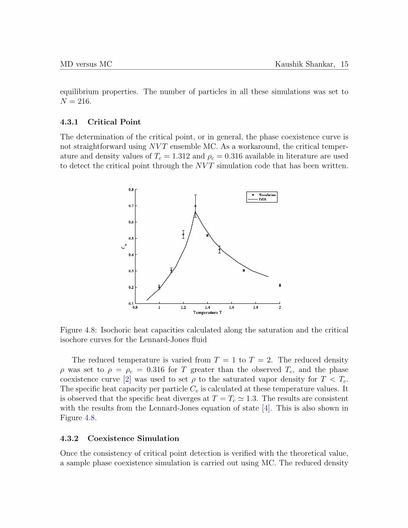
4.3.1 Critical Point

The determination of the critical point, or in general, the phase coexistence curve isnot straightforward using NV T ensemble MC. As a workaround, the critical temper-ature and density values of Tc = 1.312 and ρc = 0.316 available in literature are usedto detect the critical point through the NV T simulation code that has been written.

Figure 4.8: Isochoric heat capacities calculated along the saturation and the criticalisochore curves for the Lennard-Jones fluid

The reduced temperature is varied from T = 1 to T = 2. The reduced densityρ was set to ρ = ρc = 0.316 for T greater than the observed Tc, and the phasecoexistence curve [2] was used to set ρ to the saturated vapor density for T < Tc.The specific heat capacity per particle Cv is calculated at these temperature values. Itis observed that the specific heat diverges at T = Tc ' 1.3. The results are consistentwith the results from the Lennard-Jones equation of state [4]. This is also shown inFigure 4.8.

4.3.2 Coexistence Simulation

Once the consistency of critical point detection is verified with the theoretical value,a sample phase coexistence simulation is carried out using MC. The reduced density


was set at ρ = 0.3. Two simulations, one at T = 0.7, and the other at T = 1.5, arecarried out. A histogram of densities is obtained by dividing the simulation domaininto smaller volumes and estimating the density at each volume. The histogram plotof the densities shows phase coexistence at T = 0.7, as represented by the presence oftwo peaks in the density histogram (Figure 4.9), at ρ = 0.16 and ρ = 0.72. Althoughthese peaks do not correspond to the exact phase coexistence curve, it still givesa qualitative confirmation that two phases are coexistent. On the other hand, thehistogram of densities do not show multiple peaks at T = 1.5 > Tc. There is just asingle peak at ρ = 0.3 (Figure 4.10).

Figure 4.9: Histogram plot showing phase coexistence below critical point

Figure 4.10: Histogram plot showing no phase coexistence above critical point

The coexistence simulation was also carried out using MD at T = 0.7 and ρ = 0.3.The final configuration (generated from an animation using VMD) is shown in Figure


4.11. A low density vapor phase can be observed roughly toward the middle of thesimulation box, and a high density liquid phase can be seen near the corners ofthe box. This, once again, is a qualitative confirmation of phase coexistence. Theanimation of the MD simulation shall be made available upon request.

Figure 4.11: Final configuration of the system following MD simulation of vapor-liquidcoexistence at T = 0.7, ρ = 0.3.

4.4 Dynamic Property Prediction

Figure 4.12: MSD versus time for argon particles at T = 195K, P = 1atm


In this section, the self diffusion coefficient for argon is calculated using MD sim-ulations at different temperatures. The number of particles was fixed at N = 100.Since diffusion coefficient data are more readily available at atmospheric pressure, thedensity input to the simulation was fixed by using experimentally measured valuesof density at the given temperature and atmospheric pressure [3]. Figure 4.12 showsthe plot of the mean squared displacement (MSD) as function of time t at a reducedtemperature of T = 1.622 (195K) and atmospheric pressure. The plot accuratelycaptures the ballistic regime where the slope of the curve on a log scale has a slopeof 2 at short times. This is followed by an intermediate regime, followed by whichthe slope becomes unity at large times in the diffusion-limited regime. It is thisdiffusion-limited regime that is used for estimating diffusivity.

Figure 4.13: Self-diffusion of argon versus time at T = 195K, P = 1atm

A plot of the diffusion coefficient computed using the Einstein relation for thesame conditions as above is shown in Figure 4.13. In the diffusion-limited regime, thispredicted value becomes a constant. Uncorrelated samples of the diffusion-coefficientvalues are then averaged to compute the average and obtain an error estimate.

This process of estimating the diffusion coefficient for Argon is repeated for dif-ferent temperatures and the resulting values are compared with those available in theliterature [5]. There is a good agreement between results, as shown in Figure 4.14.

Although MC is in general a better choice for equilibrium property estimation,prediction of dynamic properties of a system like the diffusion coefficient is largelypossible only using MD simulations, as illustrated in this section. This is becauseMonte Carlo methods lack a definition of time, and instead deal with moves/sweeps.


Figure 4.14: Temperature dependence of self-diffusion coefficient of argon at 1atm

4.5 MC as a Predictor of Overdamped Brownian Dynamics

Although it was stated in the previous section that MD can predict dynamics ofa system whereas MC in general can not, there is a special case where MetropolisMC can predict dynamics. In the limit of small move sizes, it has been shown thatMC results can be connected to those from dynamic simulations. One such exampleis a study by Scarlett et al on the dynamics of colloidal crystallization using MCsimulations [6].

It is stated here without proof that MC simulations and dynamic simulationsequivalent when the move size is constrained in such a way that

K ≡ 3

8

∂U

∂x

δ

kBT<< 1 (21)

is always satisfied.MC simulations in 1D were carried out to demonstrate this equivalence. As a test

case, a system of 10, 000 non-interacting particles were simulated in the absence ofa potential energy function. This case is then essentially the free-diffusion process.Since there are no potential energy terms, there is no limit on the maximum MC movesize in this case. The initial condition of the system was a pulse at x = 0 (∼ δ(x)),and the particle positions after a time of 100 sweeps and 400 sweeps were recorded,and are shown in Figure 4.15.

The particle concentrations versus position fit a Gaussian curve, with the peakheight after 100 sweeps being twice the peak height after 400 sweeps. The standarddeviation of the curve after 400 sweeps is twice the standard deviation of the curve


Figure 4.15: Free diffusion using MC simulations

after 100 sweeps. This is consistent with the scaling observed for the standard devi-ation with respect to time. (σ ∼

√t). All one now needs to do is map these results

with the available theoretical expressions in order to get a definition for an MC sweepin terms of actual time units.

Now, since the test case gave satisfactory results, a harmonic potential was added.This is given by U = −1

2kx2. For this case, the MC move size was constrained

according to Equation 21. The parameters chosen for the study are k = 1 andkBT = 1 in reduced units. A plot of MSD versus number of sweeps from the MCsimulation was obtained, and the resulting plot was mapped with Brownian Dynamics(BD) and MD simulations to get an equivalence between MC sweeps and the dynamictime step.

Figure 4.16: MSD versus time for an overdamped Brownian harmonic oscillator usingMC and BD


Figure 4.17: MSD versus time for an overdamped Brownian harmonic oscillator usingMC and MD

From Figure 4.16, it can be seen that the MC simulations are consistent withthe result predicted by the overdamped (diffusive) Brownian dynamics simulation.However, neither the MC nor BD simulations are able to capture the ballistic regimeat short times. An MD simulation is still a more accurate representation of thedynamics in that it can capture the ballistic regime at short times. This has beenillustrated in Figure 4.17. All the three methods give rise to the same estimate forthe cage length, and match the theoretical value.

Cage length =

√kBT

k= lim

t→∞

√MSD(t) = 1 (22)

Figure 4.18: Evolution of concentration profile using MC dynamics


At steady state (long times), the particle concentration profile is consistent withthe steady state solution to the Fokker Planck equation (Boltzmann relation), as inFigure 4.18. The initial condition is a pulse of 10,000 particles at x = 5 (∼ δ(x− 5)).

5 Conclusions

MD and MC simulations were applied to simulate a Lennard-Jones fluid. Both thesesimulation methods gave identical predictions of thermodynamic properties of thesystem. Differences arise in the sampling efficiency of these methods. While MCsimulations provide a better sampling at low density, MD simulations become com-parable or marginally better than MC simulations at higher densities. This differencearises because of the ability of MC to make large unphysical moves at low densities,while the maximum allowable move size becomes smaller at higher densities, leadingto poorer sampling. The move size in MC simulations is a very significant parameterin determining the sampling efficiency of MC. A very small or very large move sizeare both not ideal choices. A move acceptance ratio around 0.4− 0.6 offers optimumsampling. Although MC is generally better for estimating equilibrium quantities, thedetermination of dynamic quantities like diffusivity is largely possible only using anMD simulation. As an illustration, the self-diffusion coefficient of argon was computedunder various conditions to give results consistent with the literature. However, mak-ing small constrained moves in an MC simulation results in an accurate predictionof dynamics. As an example, an MC simulation of the 1D overdamped Brownianharmonic oscillator was carried out to show the equivalence between BD, MD andMC simulations.


References

1. Martyna, G. J., Klein, M. L. & Tuckerman, M. Nose–Hoover chains: The canonicalensemble via continuous dynamics. The Journal of Chemical Physics 97, 2635–2643 (1992).

2. Smit, B. Phase diagrams of Lennard-Jones fluids. The Journal of Chemical Physics96, 8639–8640 (1992).

3. Lemmon, E. Thermophysical properties of fluid systems. NIST Chemistry Web-Book (1998).

4. Boda, D., Lukacs, T., Liszi, J. & Szalai, I. The isochoric-, isobaric-and saturation-heat capacities of the Lennard-Jones fluid from equations of state and MonteCarlo simulations. Fluid phase equilibria 119, 1–16 (1996).

5. Winn, E. B. The temperature dependence of the self-diffusion coefficients of argon,neon, nitrogen, oxygen, carbon dioxide, and methane. Physical Review 80, 1024(1950).

6. Scarlett, R. T., Crocker, J. C. & Sinno, T. Computational analysis of binarysegregation during colloidal crystallization with DNA-mediated interactions. TheJournal of chemical physics 132, 234705 (2010).


A Cleaner autocorrelation plot

The autocorrelation plots present in the main report are for small particle numbers.Simulations with large particle numbers or large data sets have not been carried outin this project due to time constraints in obtaining results. However, in order toshow that the sampling efficiencies based on autocorrelation functions using N = 216particles provide a reasonable estimate, a simulation was run where a larger numberof particles and more number of data points were used to give rise to a cleaner energyautocorrelation function. Figure A.1 shows the same, for N = 400, T = 1.2, ρ = 0.8.It is observed that the range of fluctuations about the zero correlation line is smallerin this case. These fluctuations are expected become lower and lower as the numberof particles in the system is increased. But this could not be verified as it requiresreally long simulation runs.

As in the main report for high density systems, the MD and MC decorrelationtimes are comparable in this case. This is confirmation that using fewer data pointsresults in a representation that is accurate, although it is noisier representation ofthe relative efficiency of MD and MC methods.

Figure A.1: A cleaner energy autocorrelation plot

a comparison between molecular dynamics and monte carlo

Documents