a comparison of spatial interpolation techniques for determining
TRANSCRIPT

A Comparison of Spatial Interpolation Techniques
For Determining Shoaling Rates of
The Atlantic Ocean Channel
By:
David L. Sterling
Thesis submitted to the Faculty of the Virginia Polytechnic Institute and State University
In partial fulfillment of the requirements for the degree of
Master of Science In
Geography
Approved:
James B. Campbell Jr., Chairman Laurence W. Carstensen Jr.
Stephen P. Prisley
May 8, 2003 Blacksburg, Virginia
Keywords: Spatial Interpolation, Multibeam Hydrographic Survey, Singlebeam
Hydrographic Survey, Shoaling, Sediment Volume
Copyright©2003, David L. Sterling

ii
A Comparison of Spatial Interpolation Techniques
For Determining Shoaling Rates of
The Atlantic Ocean Channel By:
David L. Sterling
Committee Chairperson: James B. Campbell Jr.
Geography
(Abstract)
The United States of Army Corp of Engineers (USACE) closely monitors the
changing depths of navigation channels throughout the U.S. and Western Europe. The
main issue with their surveying methodology is that the USACE surveys in linear cross
sections, perpendicular to the channel direction. Depending on the channel length and
width, these cross sections are spaced 100 – 400 feet apart, which produces large
unmapped areas within each cross section of a survey.
Using a variety of spatial interpolation methods, depths of these unmapped areas
were produced. The choice of spatial interpolator varied upon which method adequately
produced surfaces from large hydrographic survey data sets with the lowest amount of
prediction error. The data used for this research consisted of multibeam and singlebeam
surveys. These surveys were taken in a systematic manner of linear cross-sections that
produced tens of thousands of data points.
Nine interpolation techniques (inverse distance weighting, completely regularized
spline, spline with tension, thin plate spline, multiquadratic spline, inverse multiquadratic
spline, ordinary kriging, simple kriging, and universal kriging) were compared for their
ability to accurately produce bathymetric surfaces of navigation channels. Each
interpolation method was tested for effectiveness in determining depths at “unknown”
areas. The level of accuracy was tested through validation and cross validation of

iii
training and test data sets for a particular hydrographic survey.
By using interpolation, grid surfaces were created at 15, 30, 60, and 90-meter
resolution for each survey of the study site, the Atlantic Ocean Channel. These surfaces
are used to produce shoaling amounts, which are taken in the form of volumes (yd.³).
Because the Atlantic Ocean Channel is a large channel with a small gradual change in
depth, a comparison of grid resolution was conducted to determine what difference, if
any, exists between the calculated volumes from varying grid resolutions. Also, a
comparison of TIN model volume calculations was compared to grid volume estimates.
Volumes are used to determine the amount of shoaling and at what rate shoaling
is occurring in a navigation channel. Shoaling in each channel was calculated for the
entire channel length. Volumes from varying grid resolutions were produced from the
Atlantic Ocean Channel over a seven-year period from 1994-2001.
Using randomly arranged test and training datasets, spline with tension and thin
plate spline produced the mean total error when interpolating using singlebeam and
multibeam hydrographic data respectively. Thin plate spline and simple kriging
produced the lowest mean total error in full cross validation testing of entire singlebeam
and multibeam hydrographic datasets respectively.
Volume analysis of varying grid resolution indicates that finer grid resolution
provides volume estimates comparable to TIN modeling, the USACE’s technique for
determining sediment volume estimates. The coarser the resolution, the less similar the
volume estimates are in comparison to TIN modeling. All grid resolutions indicate that
the Atlantic Ocean Channel is shoaling. Using a plan depth of 53 feet, TIN modeling
displayed an annual average increase of 928,985 cubic yards of sediment from 1994 –
2001.

iv
Table of Contents
1 Introduction ................................................................................................................ 1
1.1 Statement of the Problem ...................................................................................... 1 1.2 Spatial Interpolation .............................................................................................. 7 1.3 Research Methodology.......................................................................................... 9 1.4 Justification for Research .................................................................................... 10 1.5 Research Scope and Objectives........................................................................... 11 1.6 Organization of this Thesis.................................................................................. 12
2 Literature Review..................................................................................................... 13
2.1 Overview ............................................................................................................. 13 2.2 Previous Atlantic Ocean Channel Studies ........................................................... 13 2.3 Hydrographic Survey Techniques ....................................................................... 14 2.4 Interpolation......................................................................................................... 16
2.4.1 Overview....................................................................................................... 16 2.4.2 Inverse Distance Weighting.......................................................................... 17 2.4.3 Splines........................................................................................................... 18 2.4.4 Kriging .......................................................................................................... 20
2.5 Validation and Cross Validation.......................................................................... 22 2.6 Previous Research using Hydrographic Survey Data.......................................... 24 2.7 Shoaling............................................................................................................... 25 2.8 Volume Estimation .............................................................................................. 26
3 Methodology ............................................................................................................. 29
3.1 Overview ............................................................................................................. 29 3.2 Data Gathering and Preparation .......................................................................... 29 3.3 Interpolation......................................................................................................... 32 3.4 Prediction Error Gathering .................................................................................. 34 3.5 Interpolation Methods – Initial Testing ............................................................... 35
3.5.1 Inverse Distance Weighting (IDW) .............................................................. 35 3.5.2 Spline – Completely Regularized, Tension, Multiquadratic, Inverse Multiquadratic & Thin – Plate ................................................................................... 37 3.5.3 Kriging – Ordinary, Simple, and Universal .................................................. 37
3.6 Interpolation Testing – Sensitivity Analysis ....................................................... 40 3.6.1 Randomly Arranged Samples ....................................................................... 40 3.6.2 Lowest and Highest Error Producing Interpolators ...................................... 41 3.6.3 Full Cross Validation of Singlebeam and Multibeam data........................... 41
3.7 Grid, TIN and Volume Analysis.......................................................................... 42 3.7.1 Grid and TIN Construction ........................................................................... 42 3.7.2 Volume Analysis........................................................................................... 43
4 Results ....................................................................................................................... 44

v
4.1 Overview ............................................................................................................. 44 4.2 Initial Testing....................................................................................................... 44
4.2.1 Summary statistics ........................................................................................ 44 4.2.2 Interpolation Testing..................................................................................... 45
4.3 Sensitivity Analysis ............................................................................................. 51 4.3.1 Singlebeam Sensitivity Analysis................................................................... 52 4.3.2 Multibeam Sensitivity Analysis.................................................................... 57
4.4 Sensitivity Analysis Results ................................................................................ 62 4.4.1 Paired t Tests................................................................................................. 64 4.4.2 Discussion of matched-pair t- Test ............................................................... 64
4.5 Highest and Lowest Error Producing Interpolators............................................. 67 4.6 Full Cross Validation of Singlebeam and Multibeam Data................................. 68 4.7 Final Results ........................................................................................................ 74
5 Volume Analysis ....................................................................................................... 76
5.1 Overview ............................................................................................................. 76 5.2 Volume Calculations ........................................................................................... 76
5.2.1 Grid Development......................................................................................... 77 5.2.2 Volume Estimates ......................................................................................... 80
5.3 Interpolation and Volume Error .......................................................................... 82 6 Conclusion................................................................................................................. 84
6.1 Summary.............................................................................................................. 84 6.2 Comparison of Interpolator Effectiveness by Survey Type ................................ 85
6.2.1 Singlebeam Hydrographic Survey Data........................................................ 85 6.2.2 Multibeam Hydrographic Survey Data......................................................... 86
6.3 Volume Analysis ................................................................................................. 87 6.4 Further Research and Recommendations ............................................................ 88
References........................................................................................................................ 91
VITA................................................................................................................................. 94

vi
LIST OF FIGURES Figure 1.1-1 Study Site: Atlantic Ocean Channel ..............................................3 Figure 1.1-2 Cross-sectional transects of a singlebeam
hydrographic survey .....................................................................4 Figure 2.3-1 Three-dimensional uncertainty of a measured
depth (USACE, 2002)...................................................................16
Figure 2.4.4-1 Semivariogram ............................................................................21
Figure 2.5-1 cross validation point removal ......................................................23
Figure 2.7-1 Regional siltation and geotechnical slope failure ........................26
Figure 2.8-1 Horizontal Average End Area diagram (USACE, 2002) ............27
Figure 2.8-2 Vertical Projection for average end area calculations (USACE, 2002) ........................................................28
Figure 3.2-1 Survey cross sections......................................................................30 Figure 3.3 –1 Subset module and display of test and training datasets ..........33 Figure 3.5.1-1 Geostatistical Analyst interface for IDW..................................36 Figure 3.5.1-2 IDW setup model for calculating optimal weight.....................36 Figure 3.5.2-1 Parameter optimizing feature ....................................................37 Figure 3.5.3-1 Semivariogram building .............................................................38 Figure 3.5.3-2 Kriging search neighborhood.....................................................39 Figure 4.4.1-1 Hypotheses of matched – pairs t Test ........................................64 Figure 4.6-1 Filled contour maps of estimated depth
using singlebeam survey data .....................................................70 Figure 4.6-2 Filled contour maps of estimated depth using
multibeam survey data ................................................................73 Figure 5.2-1 Cross validation of the 1994 singlebeam
hydrographic survey....................................................................77 Figure 5.2-2 Cross validation of the 1996 singlebeam
hydrographic survey....................................................................78
vii
Figure 5.2-3 Cross validation of the 1999 singlebeam hydrographic survey....................................................................78
Figure 5.2-4 Cross validation of the 2000 multibeam hydrographic survey....................................................................79 Figure 5.2-5 Cross validation of the 2001 multibeam
hydrographic survey....................................................................79
viii
List of Tables
Table 3.2-1 Data Density and survey type for all bathymetric surveys used..............................................................................................32
Table 4.2.1-1 Summary Statistics of singlebeam and multibeam data.........................................................................................45 Table 4.2.2-1 Mean Predicted Error totals in feet of initial
interpolation produced from validation of singlebeam and multibeam data.........................................................................................46
Table 4.2.2-2 RMSE values in feet of initial interpolation
produced from validation of singlebeam and multibeam data............47 Table 4.2.2-3 Mean Predicted Error totals in feet of initial
interpolation produced from cross validation of singlebeam and multibeam data .................................................................................48
Table 4.2.2-4 RMSE totals in feet of initial interpolation
produced from cross validation of singlebeam and multibeam data ............................................................................................................48
Table 4.2.2-5 Mean Total Error of initial interpolation produced from cross validation and validation
of singlebeam and multibeam data.........................................................49 Table 4.2.2-6 Ranking of interpolation methods using absolute
combined error for both singlebeam and multibeam data ..................50
Table 4.3.1-1 Summary and analytical statistics for RMSE of the singlebeam validation sensitivity analysis ...................................53
Table 4.3.1-2 Summary and analytical statistics for
MPE of the singlebeam validation sensitivity analysis .........................54 Table 4.3.1-3 Summary and analytical statistics for RMSE
of the singlebeam cross validation sensitivity analysis .........................55 Table 4.3.1-4 Summary and analytical statistics for MPE
of the singlebeam cross validation sensitivity analysis .........................56 Table 4.3.1-5 Mean Total Error of validation
and cross validation for interpolation sensitivity analysis using singlebeam data..............................................................................57

ix
Table 4.3.2-1 Summary and analytical statistics for RMSE of the multibeam validation sensitivity analysis .......................58
Table 4.3.2-2 Summary and analytical statistics for
MPE of the multibeam validation sensitivity analysis..........................59
Table 4.3.2-3 Summary and analytical statistics for RMSE of the multibeam cross validation sensitivity analysis .............60
Table 4.3.2-4 Summary and analytical statistics for
MPE of the multibeam cross validation sensitivity analysis ................61 Table 4.3.2-5 Mean Total Error of validation
and cross validation for interpolation sensitivity analysis using multibeam data ..............................................................................62
Table 4.4.2-1 Matched Pairs T - Test of the
mean total error from the singlebeam survey sensitivity analysis ......65 Table 4.4.2-2 Matched Pairs T - Test of the
mean total error from the multibeam survey sensitivity analysis .......65 Table 4.4.2-3 Dendrogram of T – Test results from
singlebeam sensitivity analysis................................................................66 Table 4.4.2-4 Dendrogram of t-test results from multibeam sensitivity analysis ................................................................66 Table 4.5-1 Mean Total Error produced from validation
and cross validation .................................................................................67 Table 4.5-2 Mean Total Error summary and analytical
statistics produced by validation and cross validation .........................68 Table 4.6-1 MPE, RMSE, and Mean Total Error of
full cross validation using 1994 singlebeam survey data......................69 Table 4.6-2 MPE, RMSE, and Mean Total Error of
full cross validation using 2001 multibeam survey data.......................72 Table 5.2.2-1 Estimated volume of sediment for TIN and varying
Grid resolution .........................................................................................80

x
Table 5.2.2-2 Estimated percentage increase of sediment volume by varying grid estimation................................................................................................ 82

xi
List of Charts
Chart 4.2.2-7 A graphical representation of each interpolation method using singlebeam and multibeam data....................................51 Chart 4.4-1 Average error of validation and cross validation for interpolation of singlebeam data .........................63 Chart 4.4-2 Average error of validation and cross validation for interpolation of multibeam data ..........................63 Chart 5.2.2-1 Volume estimates of varying grid resolution models and TIN models ..........................................................................81 Chart 5.2.2-2 Volume estimate produced by grid and TIN modeling...................................................................................................81

xii
Acknowledgements
What seemed to be a never-ending endeavor has finally come to a satisfying
finish only because of the unselfish contributions of so many. I would like to thank Dr.
Jim Campbell, Dr. Steve Prisley and Dr. Larry Grossman for their time, efforts,
encouragement and criticisms over the last three years. Each person was very beneficial
in the completion of this research and each helped me in their own unique way. I owe a
great deal of appreciation to Dr. Bill Carstensen for his contributions in the completion of
this research. Not only did he see that I complete the bulk my work in a timely fashion,
but he did a great deal of editing in a short amount of time. His efforts were well above
the call of duty and I am extremely grateful for his help and contributions towards the
completion of this thesis.
Over the last three years, I have met many individuals who have become some of
the best friends one could ever wish for. I am really thankful to many people but a
certain few were extremely instrumental in completing this thesis. I would like to thank
Justin Gorman for his statistical consulting and advice. I would like to thank fellow
geography major, Mark Dion, for providing many distractions that were sometimes
needed during this research. I would also like to thank Joe Cleary, Mel Butler and Ryan
Rantz for being great friends throughout my three years at Virginia Tech. I am truly
grateful to have met these individuals and to have spent the best time of life with. Thank
you guys.
Most importantly, I would like to thank my parents, bother and grandparents for
supporting me throughout this three-year adventure. Words can’t explain the
appreciation I have for all that you have given me. Thank you and I love all of you.

1
1 Introduction 1.1 Statement of the Problem
Over 500 million dollars are spent annually maintaining navigational waters all
over the U.S. (Pope, 2002). Most of this money spent is put towards the actual effort of
moving sediment from channels to designated disposal sites. A smaller percentage of the
allocated funds for dredging are used towards mapping and surveying of navigable water
bodies. The U.S. Army Corp of Engineers (USACE), whose main objective is to aid the
United States Navy by keeping navigation channels at adequate depth, conducts
monitoring and surveying of channels. The USACE is currently responsible for 12,000
miles of waterways and actively maintain over 900 navigation projects (USACE, 2002).
Hydrographic surveys are produced by the USACE to support dredging, flood control
and navigation projects. A variety of survey techniques are used to properly map
navigation channels, inlets, harbors, and shorelines. This research will focus mainly on
singlebeam and multibeam bathymetric survey data in a deep-water ocean navigation
channel.
The USACE has devised several methods to properly estimate the volume of
sediment that is accumulating in a channel. Documented as dredge volume computation
techniques, Average End Area calculations, Triangulated Irregular Network (TIN), and
Bin modeling are three ways that the USACE calculates sediment volume (USACE,
2002). There has been recent documentation of research that has focused on spatial
interpolation as a feasible method for sediment volume calculations. Spatial interpolation
allows point survey data to be converted into continuous contoured surfaces.
Accurate depth surveys are crucial to many aspects of maritime and military
activities. Large U.S. harbors need surveying done regularly to facilitate large ships that
enter and exit busy ports daily. The USACE’s main objective is to aid the U.S. Navy by
properly keeping channels at safe depth for passage. Because harbor water is actively
churned by large ship traffic, the movement and accumulation of sediment is often very

2
rapid in navigation channels. The Maersk Lines Suez-Class (SClass) containerships, for
example, have an overall length of 1,138 ft, a beam of 141’, and a draft of 47’ when fully
loaded. At the present time, large containerships visiting Norfolk, VA have been
restricted to a draft of about 38’, which requires the large deep draft containerships to be
only partially loaded when entering and leaving Norfolk Harbor (Hammel, Hwang,
Puglisi, Liotta, 2001). Understanding the fate of sediment in navigation channels and
proper surveying is critical for cost effective maintenance (Pope, 2002).
Given multiple sets of bathymetric survey data and using spatial interpolation,
sediment volumes will be estimated to determine the level of sediment accumulation in a
navigation channel. The navigation channel used in this research is the Atlantic Ocean
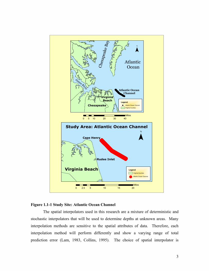
Channel, which can be seen in figure 1.1-1. The Atlantic Ocean Channel is located
offshore of Virginia Beach, Virginia in the Atlantic Ocean (See Figure 1.1-1). The
northern entrance of the channel is approximately three miles offshore of Cape Henry and
the southern entrance is located approximately ten miles offshore of Rudee Inlet, Virginia
Beach, VA (USACE, 1986). The Atlantic Ocean Channel is the main shipping channel
that leads into the Chesapeake Bay, one of the largest estuaries in the world. This
channel is 10.6 miles long and has a width of over 1,000 feet (Berger, et al, 1985).
The Atlantic Ocean Channel is part of the Norfolk Harbor System. Norfolk Harbor
is one of the world’s deepest natural harbors and also houses the Norfolk Oceania Naval
Base, one of the world’s largest naval bases (Global Security, 2002). The original plan
depth (depth required for safe passage) was 57 feet deep and over time, the Atlantic
Ocean Channel has slowly been accumulating sediment due to tidal, storm and ship
produced currents.
3
Atlantic OceanC
hesa
peak
e B
ay
James River
Virginia Beach
Chesapeake
Atlantic Ocean Channel
Norfolk
LegendAtlantic Ocean Channel
Virginia Counties
¯
&&&&&&&&&&&&&&&&&&&&&&&&&&&&&&&&&&&&&&&&&&&&&&&&&&&&&&&&&&&&&&&&&&&&&&&&&&&&&&&&&&&&&&&&&&&&&&&&&&&&&&&&&&&&&&&&&&&&&&&&&&&&&&&&&&&&&&&&&&&&&&&&&&&&&&&&&&&&&&&&&&&&&&&&&&&&&&&&&&&&&&&&&&&&&&&&&&&&&&&&&&&&&&&&&&&&&&&&&&&&&&&&&&&&&&&&&&&&&&&&&&&&&&&&&&&&&&&&&&&&&&&&&&&&&&&&&&&&&&&&&&&&&&&&&&&&&&&&&&&&&&&&&&&&&&&&&&&&&&&&&&&&&&&&&&&&&&&&&&&&&&&&&&&&&&&&&&&&&&&&&&&&&&&&&&&&&&&&&&&&&&&&&&&&&&&&&&&&&&&&&&&&&&&&&&&&&&&&&&&&&&&&&&&&&&&&&&&&&&&&&&&&&&&&&&&&&&&&&&&&&&&&&&&&&&&&&&&&&&&&&&&&&&&&&&&&&&&&&&&&&&&&&&&&&&&&&&&&&&&&&&&&&&&&&&&&&&&&&&&&&&&&&&&&&&&&&&&&&&&&&&&&&&&&&&&&&&&&&&&&&&&&&&&&&&&&&&&&&&&&&&&&&&&&&&&&&&&&&&&&&&&&&&&&&&&&&&&&&&&&&&&&&&&&&&&&&&&&&&&&&&&&&&&&&&&&&&&&&&&&&&&&&&&&&&&&&&&&&&&&&&&&&&&&&&&&&&&&&&&&&&&&&&&&&&&&&&&&&&&&&&&&&&&&&&&&&&&&&&&&&&&&&&&&&&&&&&&&&&&&&&&&&&&&&&&&&&&&&&&&&&&&&&&&&&&&&&&&&&&&&&&&&&&&&&&&&&&&&&&&&&&&&&&&&&&&&&&&&&&&&&&&&&&&&&&&&&&&&&&&&&&&&&&&&&&&&&&&&&&&&&&&&&&&&&&&&&&&&&&&&&&&&&&&&&&&&&&&&&&&&&&&&&&&&&&&&&&&&&&&&&&&&&&&&&&&&&&&&&&&&&&&&&&&&&&&&&&&&&&&&&&&&&&&&&&&&&&&&&&&&&&&&&&&&&&&&&&&&&&&&&&&&&&&&&&&&&&&&&&&&&&&&&&&&&&&&&&&&&&&&&&&&&&&&&&&&&&&&&&&&&&&&&&&&&&&&&&&&&&&&&&&&&&&&&&&&&&&&&&&&&&&&&&&&&&&&&&&&&&&&&&&&&&&&&&&&&&&&&&&&&&&&&&&&&&&&&&&&&&&&&&&&&&&&&&&&&&&&&&&&&&&&&&&&&&&&&&&&&&&&&&&&&&&&&&&&&&&&&&&&&&&&&&&&&&&&&&&&&&&&&&&&&&&&&&&&&&&&&&&&&&&&&&&&&&&&&&&&&&&&&&&&&&&&&&&&&&&&&&&&&&&&&&&&&&&&&&&&&&&&&&&&&&&&&&&&&&&&&&&&&&&&&&&&&&&&&&&&&&&&&&&&&&&&&&&&&&&&&&&&&&&&&&&&&&&&&&&&&&&&&&&&&&&&&&&&&&&&&&&&&&&&&&&&&&&&&&&&&&&&&&&&&&&&&&&&&&&&&&&&&&&&&&&&&&&&&&&&&&&&&&&&&&&&&&&&&&&&&&&&&&&&&&&&&&&&&&&&&&&&&&&&&&&&&&&&&&&&&&&&&&&&&&&&&&&&&&&&&&&&&&&&&&&&&&&&&&&&&&&&&&&&&&&&&&&&&&&&&&&&&&&&&&&&&&&&&&&&&&&&&&&&&&&&&&&&&&&&&&&&&&&&&&&&&&&&&&&&&&&&&&&&&&&&&&&&&&&&&&&&&&&&&&&&&&&&&&&&&&&&&&&&&&&&&&&&&&&&&&&&&&&&&&&&&&&&&&&&&&&&&&&&&&&&&&&&&&&&&&&&&&&&&&&&&&&&&&&&&&&&&&&&&&&&&&&&&&&&&&&&&&&&&&&&&&&&&&&&&&&&&&&&&&&&&&&&&&&&&&&&&&&&&&&&&&&&&&&&&&&&&&&&&&&&&&&&&&&&&&&&&&&&&&&&&&&&&&&&&&&&&&&&&&&&&&&&&&&&&&&&&&&&&&&&&&&&&&&&&&&&&&&&&&&&&&&&&&&&&&&&&&&&&&&&&&&&&&&&&&&&&&&&&&&&&&&&&&&&&&&&&&&&&&&&&&&&&&&&&&&&&&&&&&&&&&&&&&&&&&&&&&&&&&&&&&&&&&&&&&&&&&&&&&&&&&&&&&&&&&&&&&&&&&&&&&&&&&&&&&&&&&&&&&&&&&&&&&&&&&&&&&&&&&&&&&&&&&&&&&&&&&&&&&&&&&&&&&&&&&&&&&&&&&&&&&&&&&&&&&&&&&&&&&&&&&&&&&&&&&&&&&&&&&&&&&&&&&&&&&&&&&&&&&&&&&&&&&&&&&&&&&&&&&&&&&&&&&&&&&&&&&&&&&&&&&&&&&&&&&&&&&&&&&&&&&&&&&&&&&&&&&&&&&&&&&&&&&&&&&&&&&&&&&&&&&&&&&&&&&&&&&&&&&&&&&&&&&&&&&&&&&&&&&&&&&&&&&&&&&&&&&&&&&&&&&&&&&&&&&&&&&&&&&&&&&&&&&&&&&&&&&&&&&&&&&&&&&&&&&&&&&&&&&&&&&&&&&&&&&&&&&&&&&&&&&&&&&&&&&&&&&&&&&&&&&&&&&&&&&&&&&&&&&&&&&&&&&&&&&&&&&&&&&&&&&&&&&&&&&&&&&&&&&&&&&&&&&&&&&&&&&&&&&&&&&&&&&&&&&&&&&&&&&&&&&&&&&&&&&&&&&&&&&&&&&&&&&&&&&&&&&&&&&&&&&&&&&&&&&&&&&&&&&&&&&&&&&&&&&&&&&&&&&&&&&&&&&&&&&&&&&&&&&&&&&&&&&&&&&&&&&&&&&&&&&&&&&&&&&&&&&&&&&&&&&&&&&&&&&&&&&&&&&&&&&&&&&&&&&&&&&&&&&&&&&&&&&&&&&&&&&&&&&&&&&&&&&&&&&&&&&&&&&&&&&&&&&&&&&&&&&&&&&&&&&&&&&&&&&&&&&&&&&&&&&&&&&&&&&&&&&&&&&&&&&&&&&&&&&&&&&&&&&&&&&&&&&&&&&&&&&&&&&&&&&&&&&&&&&&&&&&&&&&&&&&&&&&&&&&&&&&&&&&&&&&&&&&&&&&&&&&&&&&&&&&&&&&&&&&&&&&&&&&&&&&&&&&&&&&&&&&&&&&&&&&&&&&&&&&&&&&&&&&&&&&&&&&&&&&&&&&&&&&&&&&&&&&&&&&&&&&&&&&&&&&&&&&&&&&&&&&&&&&&&&&&&&&&&&&&&&&&&&&&&&&&&&&&&&&&&&&&&&&&&&&&&&&&&&&&&&&&&&&&&&&&&&&&&&&&&&&&&&&&&&&&&&&&&&&&&&&&&&&&&&&&&&&&&&&&&&&&&&&&&&&&&&&&&&&&&&&&&&&&&&&&&&&&&&&&&&&&&&&&&&&&&&&&&&&&&&&&&&&&&&&&&&&&&&&&&&&&&&&&&&&&&&&&&&&&&&&&&&&&&&&&&&&&&&&&&&&&&&&&&&&&&&&&&&&&&&&&&&&&&&&&&&&&&&&&&&&&&&&&&&&&&&&
&&&&&&&&&&&&&&&&&&&&&&&&&&&&&&&&&&&&&&&&&&&&&&&&&&&&&&&&&&&&&&&&&&&&&&&&&&&&&&&&&&&&&&&&&&&&&&&&&&&&&&&&&&&&&&&&&&&&&&&&&&&&&&&&&&&&&&&&&&&&&&&&&&&&&&&&&&&&&&&&&&&&&&&&&&&&&&&&&&&&&&&&&&&&&&&&&&&&&&&&&&&&&&&&&&&&&&&&&&&&&&&&&&&&&&&&&&&&&&&&&&&&&&&&&&&&&&&&&&&&&&&&&&&&&&&&&&&&&&&&&&&&&&&&&&&&&&&&&&&&&&&&&&&&&&&&&&&&&&&&&&&&&&&&&&&&&&&&&&&&&&&&&&&&&&&&&&&&&&&&&&&&&&&&&&&&&&&&&&&&&&&&&&&&&&&&&&&&&&&&&&&&&&&&&&&&&&&&&&&&&&&&&&&&&&&&&&&&&&&&&&&&&&&&&&&&&&&&&&&&&&&&&&&&&&&&&&&&&&&&&&&&&&&&&&&&&&&&&&&&&&&&&&&&&&&&&&&&&&&&&&&&&&&&&&&&&&&&&&&&&&&&&&&&&&&&&&&&&&&&&&&&&&&&&&&&&&&&&&&&&&&&&&&&&&&&&&&&&&&&&&&&&&&&&&&&&&&&&&&&&&&&&&&&&&&&&&&&&&&&&&&&&&&&&&&&&&&&&&&&&&&&&&&&&&&&&&&&&&&&&&&&&&&&&&&&&&&&&&&&&&&&&&&&&&&&&&&&&&&&&&&&&&&&&&&&&&&&&&&&&&&&&&&&&&&&&&&&&&&&&&&&&&&&&&&&&&&&&&&&&&&&&&&&&&&&&&&&&&&&&&&&&&&&&&&&&&&&&&&&&&&&&&&&&&&&&&&&&&&&&&&&&&&&&&&&&&&&&&&&&&&&&&&&&&&&&&&&&&&&&&&&&&&&&&&&&&&&&&&&&&&&&&&&&&&&&&&&&&&&&&&&&&&&&&&&&&&&&&&&&&&&&&&&&&&&&&&&&&&&&&&&&&&&&&&&&&&&&&&&&&&&&&&&&&&&&&&&&&&&&&&&&&&&&&&&&&&&&&&&&&&&&&&&&&&&&&&&&&&&&&&&&&&&&&&&&&&&&&&&&&&&&&&&&&&&&&&&&&&&&&&&&&&&&&&&&&&&&&&&&&&&&&&&&&&&&&&&&&&&&&&&&&&&&&&&&&&&&&&&&&&&&&&&&&&&&&&&&&&&&&&&&&&&&&&&&&&&&&&&&&&&&&&&&&&&&&&&&&&&&&&&&&&&&&&&&&&&&&&&&&&&&&&&&&&&&&&&&&&&&&&&&&&&&&&&&&&&&&&&&&&&&&&&&&&&&&&&&&&&&&&&&&&&&&&&&&&&&&&&&&&&&&&&&&&&&&&&&&&&&&&&&&&&&&&&&&&&&&&&&&&&&&&&&&&&&&&&&&&&&&&&&&&&&&&&&&&&&&&&&&&&&&&&&&&&&&&&&&&&&&&&&&&&&&&&&&&&&&&&&&&&&&&&&&&&&&&&&&&&&&&&&&&&&&&&&&&&&&&&&&&&&&&&&&&&&&&&&&&&&&&&&&&&&&&&&&&&&&&&&&&&&&&&&&&&&&&&&&&&&&&&&&&&&&&&&&&&&&&&&&&&&&&&&&&&&&&&&&&&&&&&&&&&&&&&&&&&&&&&&&&&&&&&&&&&&&&&&&&&&&&&&&&&&&&&&&&&&&&&&&&&&&&&&&&&&&&&&&&&&&&&&&&&&&&&&&&&&&&&&&&&&&&&&&&&&&&&&&&&&&&&&&&&&&&&&&&&&&&&&&&&&&&&&&&&&&&&&&&&&&&&&&&&&&&&&&&&&&&&&&&&&&&&&&&&&&&&&&&&&&&&&&&&&&&&&&&&&&&&&&&&&&&&&&&&&&&&&&&&&&&&&&&&&&&&&&&&&&&&&&&&&&&&&&&&&&&&&&&&&&&&&&&&&&&&&&&&&&&&&&&&&&&&&&&&&&&&&&&&&&&&&&&&&&&&&&&&&&&&&&&&&&&&&&&&&&&&&&&&&&&&&&&&&&&&&&&&&&&&&&&&&&&&&&&&&&&&&&&&&&&&&&&&&&&&&&&&&&&&&&&&&&&&&&&&&&&&&&&&&&&&&&&&&&&&&&&&&&&&&&&&&&&&&&&&&&&&&&&&&&&&&&&&&&&&&&&&&&&&&&&&&&&&&&&&&&&&&&&&&&&&&&&&&&&&&&&&&&&&&&&&&&&&&&&&&&&&&&&&&&&&&&&&&&&&&&&&&&&&&&&&&&&&&&&&&&&&&&&&&&&&&&&&&&&&&&&&&&&&&&&&&&&&&&&&&&&&&&&&&&&&&&&&&&&&&&&&&&&&&&&&&&&&&&&&&&&&&&&&&&&&&&&&&&&&&&&&&&&&&&&&&&&&&&&&&&&&&&&&&&&&&&&&&&&&&&&&&&&&&&&&&&&&&&&&&&&&&&&&&&&&&&&&&&&&&&&&&&&&&&&&&&&&&&&&&&&&&&&&&&&&&&&&&&&&&&&&&&&&&&&&&&&&&&&&&&&&&&&&&&&&&&&&&&&&&&&&&&&&&&&&&&&&&&&&&&&&&&&&&&&&&&&&&&&&&&&&&&&&&&&&&&&&&&&&&&&&&&&&&&&&&&&&&&&&&&&&&&&&&&&&&&&&&&&&&&&&&&&&&&&&&&&&&&&&&&&&&&&&&&&&&&&&&&&&&&&&&&&&&&&&&&&&&&&&&&&&&&&&&&&&&&&&&&&&&&&&&&&&&&&&&&&&&&&&&&&&&&&&&&&&&&&&&&&&&&&&&&&&&&&&&&&&&&&&&&&&&&&&&&&&&&&&&&&&&&&&&&&&&&&&&&&&&&&&&&&&&&&&&&&&&&&&&&&&&&&&&&&&&&&&&&&&&&&&&&&&&&&&&&&&&&&&&&&&&&&&&&&&&&&&&&&&&&&&&&&&&&&&&&&&&&&&&&&&&&&&&&&&&&&&&&&&&&&&&&&&&&&&&&&&&&&&&&&&&&&&&&&&&&&&&&&&&&&&&&&&&&&&&&&&&&&&&&&&&&&&&&&&&&&&&&&&&&&&&&&&&&&&&&&&&&&&&&&&&&&&&&&&&&&&&&&&&&&&&&&&&&&&&&&&&&&&&&&&&&&&&&&&&&&&&&&&&&&&&&&&&&&&&&&&&&&&&&&&&&&&&&&&&&&&&&&&&&&&&&&&&&&&&&&&&&&&&&&&&&&&&&&&&&&&&&&&&&&&&&&&&&&&&&&&&&&&&&&&&&&&&&&&&&&&&&&&&&&&&&&&&&&&&&&&&&&&&&&&&&&&&&&&&&&&&&&&&&&&&&&&&&&&&&&&&&&&&&&&&&&&&&&&&&&&&&&&&&&&&&&&&&&&&&&&&&&&&&&&&&&&&&&&&&&&&&&&&&&&&&&&&&&&&&&&&&&&&&&&&&&&&&&&&&&&&&&&&&&&&&&&&&&&&&&&&&&&&&&&&&&&&&&&&&&&&&&&&&&&&&&&&&&&&&&&&&&&&&&&&&&&&&&&&&&&&&&&&&&&&&&&&&&&&&&&&&&&&&&&&&&&&&&&&&&&&&&&&&&&&&&&&&&&&&&&&&&&&&&&&&&&&&&&&&&&&&&&&&&&&&&&&&&&&&&&&&&&&&&&&&&&&&&&&&&&&&&&&&&&&&&&&&&&&&&&&&&&&&&&&&&&&&&&&&&&&&&&&&&&&&&&&&&&&&&&&&&&&&&&&&&&&&&&&&&&&&&&&&&&&&&&&&&&&&&&&&&&&&&&&&&&&&&&&&&&&&&&&&&&&&&&&&&&&&&&&&&&&&&&&&&&&&&&&&&&&&&&&&&&&&&&&&&&&&&&&&&&&&&&&&&&&&&&&&&&&&&&&&&&&&&&&&&&&&&&&&&&&&&&&&&&&&&&&&&&&&&&&&&&&&&&&&&&&&&&&&&&&&&&&&&&&&&&&&&&&&&&&&&&&&&&&&&&&&&&&&&&&&&&&&&&&&&&&&&&&&&&&&&&&&&&&&&&&&&&&&&&&&&&&&&&&&&&&&&&&&&&&&&&&&&&&&&&&&&&&&&&&&&&&&&&&&&&&&&&&&&&&&&&&&&&&&&&&&&&&&&&&&&&&&&&&&&&&&&&&&&&&&&&&&&&&&&&&&&&&&&&&&&&&&&&&&&&&&&&&&&&&&&&&&&&&&&&&&&&&&&&&&&&&&&&&&&&&&&&&&&&&&&&&&&&&&&&&&&&&&&&&&&&&&&&&&&&&&&&&&&&&&&&&&&&&&&&&&&&&&&&&&&&&&&&&&&&&&&&&&&&&&&&&&&&&&&&&&&&&&&&&&&&&&&&&&&&&&&&&&&&&&&&&&&&&&&&&&&&&&&&&&&&&&&&&&&&&&&&&&&&&&&&&&&&&&&&&&&&&&&&&&&&&&&&&&&&&&&&&&&&&&&&&&&&&&&&&&&&&&&&&&&&&&&&&&&&&&&&&&&&&&&&&&&&&&&&&&&&&&&&&&&&&&&&&&&&&&&&&&&&&&&&&&&&&&&&&&&&&&&&&&&&&&&&&&&&&&&&&&&&&&&&&&&&&&&&&&&&&&&&&&&&&&&&&&&&&&&&&&&&&&&&&&&&&&&&&&&&&&&&&&&&&&&&&&&&&&&&&&&&&&&&&&&&&&&&&&&&&&&&&&&&&&&&&&&&&&&&&&&&&&&&&&&&&&&&&&&&&&&&&&&&&&&&&&&&&&&&&&&&&&&&&&&&&&&&&&&&&&&&&&&&&&&&&&&&&&&&&&&&&&&&&&&&&&&&&&&&&&&&&&&&&&&&&&&&&&&&&&&&&&&&&&&&&&&&&&&&&&&&&&&&&&&&&&&&&&&&&&&&&&&&&&&&&&&&&&&&&&&&&&&&&&&&&&&&&&&&&&&&&&&&&&&&&&&&&&&&&&&&&&&&&&&&&&&&&&&&&&&&&&&&&&&&&&&&&&&&&&&&&&&&&&&&&&&&&&&&&&&&&&&&&&&&&&&&&&&&&&&&&&&&&&&&&&&&&&&&&&&&&&&&&&&&&&&&&&&&&&&&&&&&&&&&&&&&&&&&&&&&&&&&&&&&&&&&&&&&&&&&&&&&&&&&&&&&&&&&&&&&&&&&&&&&&&&&&&&&&&&&&&&&&&&&&&&&&&&&&&&&&&&&&&&&&&&&&&&&&&&&&&&&&&&&&&&&&&&&&&&&&&&&&&&&&&&&&&&&&&&&&&&&&&&&&&&&&&&&&&&&&&&&&&&&&&&&&&&&&&&&&&&&&&&&&&&&&&&&&&&&&&&&&&&&&&&&&&&&&&&&&&&&&&&&&&&&&&&&&&&&&&&&&&&&&&&&&&&&&&&&&&&&&&&&&&&&&&&&&&&&&&&&&&&&&&&&&&&&&&&&&&&&&&&&&&&&&&&&&&&&&&&&&&&&&&&&&&&&&&&&&&&&&&&&&&&&&&&&&&&&&&&&&&&&&&&&&&&&&&&&&&&&&&&&&&&&&&&&&&&&&&&&&&&&&&&&&&&&&&&&&&&&&&&&&&&&&&&&&&&&&&&&&&&&&&&&&&&&&&&&&&&&&&&&&&&&&&&&&&&&&&&&&&&&&&&&&&&&&&&&&&&&&&&&&&&&&&&&&&&&&&&&&&&&&&&&&&&&&&&&&&&&&&&&&&&&&&&&&&&&&&&&&&&&&&&&&&&&&&&&&&&&&&&&&&&&&&&&&&&&&&&&&&&&&&&&&&&&&&&&&&&&&&&&&&&&&&&&&&&&&&&&&&&&&&&&&&&&&&&&&&&&&&&&&&&&&&&&&&&&&&&&&&&&&&&&&&&&&&&&&&&&&&&&&&&&&&&&&&&&&&&&&&&&&&&&&&&&&&&&&&&&&&&&&&&&&&&&&&&&&&&&&&&&&&&&&&&&&&&&&&&&&&&&&&&&&&&&&&&&&&&&&&&&&&&&&&&&&&&&&&&&&&&&&&&&&&&&&&&&&&&&&&&&&&&&&&&&&&&&&&&&&&&&&&&&&&&&&&&&&&&&&&&&&&&&&&&&&&&&&&&&&&&&&&&&&&&&&&&&&&&&&&&&&&&&&&&&&&&&&&&&&&&&&&&&&&&&&&&&&&&&&&&&&&&&&&&&&&&&&&&&&&&&&&&&&&&&&&&&&&&&&&&&&&&&&&&&&&&&&&&&&&&&&&&&&&&&&&&&&&&&&&&&&&&&&&&&&&&&&&&&&&&&&&&&&&&&&&&&&&&&&&&&&&&&&&&&&&&&&&&&&&&&&&&&&&&&&&&&&&&&&&&&&&&&&&&&&&&&&&&&&&&&&&&&&&&&&&&&&&&&&&&&&&&&&&&&&&&&&&&&&&&&&&&&&&&&&&&&&&&&&&&&&&&&&&&&&&&&&&&&&&&&&&&&&&&&&&&&&&&&&&&&&&&&&&&&&&&&&&&&&&&&&&&&&&&&&&&&&&&&&&&&&&&&&&&&&&&&
&&&&&&&&&&&&&&&&&&&&&&&&&&&&&&&&&&&&&&&&&&&&&&&&&&&&&&&&&&&&&&&&&&&&&&&&&&&&&&&&&&&&&&&&&&&&&&&&&&&&&&&&&&&&&&&&&&&&&&&&&&&&&&&&&&&&&&&&&&&&&&&&&&&&&&&&&&&&&&&&&&&&&&&&&&&&&&&&&&&&&&&&&&&&&&&&&&&&&&&&&&&&&&&&&&&&&&&&&&&&&&&&&&&&&&&&&&&&&&&&&&&&&&&&&&&&&&&&&&&&&&&&&&&&&&&&&&&&&&&&&&&&&&&&&&&&&&&&&&&&&&&&&&&&&&&&&&&&&&&&&&&&&&&&&&&&&&&&&&&&&&&&&&&&&&&&&&&&&&&&&&&&&&&&&&&&&&&&&&&&&&&&&&&&&&&&&&&&&&&&&&&&&&&&&&&&&&&&&&&&&&&&&&&&&&&&&&&&&&&&&&&&&&&&&&&&&&&&&&&&&&&&&&&&&&&&&&&&&&&&&&&&&&&&&&&&&&&&&&&&&&&&&&&&&&&&&&&&&&&&&&&&&&&&&&&&&&&&&&&&&&&&&&&&&&&&&&&&&&&&&&&&&&&&&&&&&&&&&&&&&&&&&&&&&&&&&&&&&&&&&&&&&&&&&&&&&&&&&&&&&&&&&&&&&&&&&&&&&&&&&&&&&&&&&&&&&&&&&&&&&&&&&&&&&&&&&&&&&&&&&&&&&&&&&&&&&&&&&&&&&&&&&&&&&&&&&&&&&&&&&&&&&&&&&&&&&&&&&&&&&&&&&&&&&&&&&&&&&&&&&&&&&&&&&&&&&&&&&&&&&&&&&&&&&&&&&&&&&&&&&&&&&&&&&&&&&&&&&&&&&&&&&&&&&&&&&&&&&&&&&&&&&&&&&&&&&&&&&&&&&&&&&&&&&&&&&&&&&&&&&&&&&&&&&&&&&&&&&&&&&&&&&&&&&&&&&&&&&&&&&&&&&&&&&&&&&&&&&&&&&&&&&&&&&&&&&&&&&&&&&&&&&&&&&&&&&&&&&&&&&&&&&&&&&&&&&&&&&&&&&&&&&&&&&&&&&&&&&&&&&&&&&&&&&&&&&&&&&&&&&&&&&&&&&&&&&&&&&&&&&&&&&&&&&&&&&&&&&&&&&&&&&&&&&&&&&&&&&&&&&&&&&&&&&&&&&&&&&&&&&&&&&&&&&&&&&&&&&&&&&&&&&&&&&&&&&&&&&&&&&&&&&&&&&&&&&&&&&&&&&&&&&&&&&&&&&&&&&&&&&&&&&&&&&&&&&&&&&&&&&&&&&&&&&&&&&&&&&&&&&&&&&&&&&&&&&&&&&&&&&&&&&&&&&&&&&&&&&&&&&&&&&&&&&&&&&&&&&&&&&&&&&&&&&&&&&&&&&&&&&&&&&&&&&&&&&&&&&&&&&&&&&&&&&&&&&&&&&&&&&&&&&&&&&&&&&&&&&&&&&&&&&&&&&&&&&&&&&&&&&&&&&&&&&&&&&&&&&&&&&&&&&&&&&&&&&&&&&&&&&&&&&&&&&&&&&&&&&&&&&&&&&&&&&&&&&&&&&&&&&&&&&&&&&&&&&&&&&&&&&&&&&&&&&&&&&&&&&&&&&&&&&&&&&&&&&&&&&&&&&&&&&&&&&&&&&&&&&&&&&&&&&&&&&&&&&&&&&&&&&&&&&&&&&&&&&&&&&&&&&&&&&&&&&&&&&&&&&&&&&&&&&&&&&&&&&&&&&&&&&&&&&&&&&&&&&&&&&&&&&&&&&&&&&&&&&&&&&&&&&&&&&&&&&&&&&&&&&&&&&&&&&&&&&&&&&&&&&&&&&&&&&&&&&&&&&&&&&&&&&&&&&&&&&&&&&&&&&&&&&&&&&&&&&&&&&&&&&&&&&&&&&&&&&&&&&&&&&&&&&&&&&&&&&&&&&&&&&&&&&&&&&&&&&&&&&&&&&&&&&&&&&&&&&&&&&&&&&&&&&&&&&&&&&&&&&&&&&&&&&&&&&&&&&&&&&&&&&&&&&&&&&&&&&&&&&&&&&&&&&&&&&&&&&&&&&&&&&&&&&&&&&&&&&&&&&&&&&&&&&&&&&&&&&&&&&&&&&&&&&&&&&&&&&&&&&&&&&&&&&&&&&&&&&&&&&&&&&&&&&&&&&&&&&&&&&&&&&&&&&&&&&&&&&&&&&&&&&&&&&&&&&&&&&&&&&&&&&&&&&&&&&&&&&&&&&&&&&&&&&&&&&&&&&&&&&&&&&&&&&&&&&&&&&&&&&&&&&&&&&&&&&&&&&&&&&&&&&&&&&&&&&&&&&&&&&&&&&&&&&&&&&&&&&&&&&&&&&&&&&&&&&&&&&&&&&&&&&&&&&&&&&&&&&&&&&&&&&&&&&&&&&&&&&&&&&&&&&&&&&&&&&&&&&&&&&&&&&&&&&&&&&&&&&&&&&&&&&&&&&&&&&&&&&&&&&&&&&&&&&&&&&&&&&&&&&&&&&&&&&&&&&&&&&&&&&&&&&&&&&&&&&&&&&&&&&&&&&&&&&&&&&&&&&&&&&&&&&&&&&&&&&&&&&&&&&&&&&&&&&&&&&&&&&&&&&&&&&&&&&&&&&&&&&&&&&&&&&&&&&&&&&&&&&&&&&&&&&&&&&&&&&&&&&&&&&&&&&&&&&&&&&&&&&&&&&&&&&&&&&&&&&&&&&&&&&&&&&&&&&&&&&&&&&&&&&&&&&&&&&&&&&&&&&&&&&&&&&&&&&&&&&&&&&&&&&&&&&&&&&&&&&&&&&&&&&&&&&&&&&&&&&&&&&&&&&&&&&&&&&&&&&&&&&&&&&&&&&&&&&&&&&&&&&&&&&&&&&&&&&&&&&&&&&&&&&&&&&&&&&&&&&&&&&&&&&&&&&&&&&&&&&&&&&&&&&&&&&&&&&&&&&&&&&&&&&&&&&&&&&&&&&&&&&&&&&&&&&&&&&&&&&&&&&&&&&&&&&&&&&&&&&&&&&&&&&&&&&&&&&&&&&&&&&&&&&&&&&&&&&&&&&&&&&&&&&&&&&&&&&&&&&&&&&&&&&&&&&&&&&&&&&&&&&&&&&&&&&&&&&&&&&&&&&&&&&&&&&&&&&&&&&&&&&&&&&&&&&&&&&&&&&&&&&&&&&&&&&&&&&&&&&&&&&&&&&&&&&&&&&&&&&&&&&&&&&&&&&&&&&&&&&&&&&&&&&&&&&&&&&&&&&&&&&&&&&&&&&&&&&&&&&&&&&&&&&&&&&&&&&&&&&&&&&&&&&&&&&&&&&&&&&&&&&&&&&&&&&&&&&&&&&&&&&&&&&&&&&&&&&&&&&&&&&&&&&&&&&&&&&&&&&&&&&&&&&&&&&&&&&&&&&&&&&&&&&&&&&&&&&&&&&&&&&&&&&&&&&&&&&&&&&&&&&&&&&&&&&&&&&&&&&&&&&&&&&&&&&&&&&&&&&&&&&&&&&&&&&&&&&&&&&&&&&&&&&&&&&&&&&&&&&&&&&&&&&&&&&&&&&&&&&&&&&&&&&&&&&&&&&&&&&&&&&&&&&&&&&&&&&&&&&&&&&&&&&&&&&&&&&&&&&&&&&&&&&&&&&&&&&&&&&&&&&&&&&&&&&&&&&&&&&&&&&&&&&&&&&&&&&&&&&&&&&&&&&&&&&&&&&&&&&&&&&&&&&&&&&&&&&&&&&&&&&&&&&&&&&&&&&&&&&&&&&&&&&&&&&&&&&&&&&&&&&&&&&&&&&&&&&&&&&&&&&&&&&&&&&&&&&&&&&&&&&&&&&&&&&&&&&&&&&&&&&&&&&&&&&&&&&&&&&&&&&&&&&&&&&&&&&&&&&&&&&&&&&&&&&&&&&&&&&&&&&&&&&&&&&&&&&&&&&&&&&&&&&&&&&&&&&&&&&&&&&&&&&&&&&&&&&&&&&&&&&&&&&&&&&&&&&&&&&&&&&&&&&&&&&&&&&&&&&&&&&&&&&&&&&&&&&&&&&&&&&&&&&&&&&&&&&&&&&&&&&&&&&&&&&&&&&&&&&&&&&&&&&&&&&&&&&&&&&&&&&&&&&&&&&&&&&&&&&&&&&&&&&&&&&&&&&&&&&&&&&&&&&&&&&&&&&&&&&&&&&&&&&&&&&&&&&&&&&&&&&&&&&&&&&&&&&&&&&&&&&&&&&&&&&&&&&&&&&&&&&&&&&&&&&&&&&&&&&&&&&&&&&&&&&&&&&&&&&&&&&&&&&&&&&&&&&&&&&&&&&&&&&&&&&&&&&&&&&&&&&&&&&&&&&&&&&&&&&&&&&&&&&&&&&&&&&&&&&&&&&&&&&&&&&&&&&&&&&&&&&&&&&&&&&&&&&&&&&&&&&&&&&&&&&&&&&&&&&&&&&&&&&&&&&&&&&&&&&&&&&&&&&&&&&&&&&&&&&&&&&&&&&&&&&&&&&&&&&&&&&&&&&&&&&&&&&&&&&&&&&&&&&&&&&&&&&&&&&&&&&&&&&&&&&&&&&&&&&&&&&&&&&&&&&&&&&&&&&&&&&&&&&&&&&&&&&&&&&&&&&&&&&&&&&&&&&&&&&&&&&&&&&&&&&&&&&&&&&&&&&&&&&&&&&&&&&&&&&&&&&&&&&&&&&&&&&&&&&&&&&&&&&&&&&&&&&&&&&&&&&&&&&&&&&&&&&&&&&&&&&&&&&&&&&&&&&&&&&&&&&&&&&&&&&&&&&&&&&&&&&&&&&&&&&&&&&&&&&&&&&&&&&&&&&&&&&&&&&&&&&&&&&&&&&&&&&&&&&&&&&&&&&&&&&&&&&&&&&&&&&&&&&&&&&&&&&&&&&&&&&&&&&&&&&&&&&&&&&&&&&&&&&&&&&&&&&&&&&&&&&&&&&&&&&&&&&&&&&&&&&&&&&&&&&&&&&&&&&&&&&&&&&&&&&&&&&&&&&&&&&&&&&&&&&&&&&&&&&&&&&&&&&&&&&&&&&&&&&&&&&&&&&&&&&&&&&&&&&&&&&&&&&&&&&&&&&&&&&&&&&&&&&&&&&&&&&&&&&&&&&&&&&&&&&&&&&&&&&&&&&&&&&&&&&&&&&&&&&&&&&&&&&&&&&&&&&&&&&&&&&&&&&&&
&&&&&&&&&&&&&&&&&&&&&&&&&&&&&&&&&&&&&&&&&&&&&&&&&&&&&&&&&&&&&&&&&&&&&&&&&&&&&&&&&&&&&&&&&&&&&&&&&&&&&&&&&&&&&&&&&&&&&&&&&&&&&&&&&&&&&&&&&&&&&&&&&&&&&&&&&&&&&&&&&&&&&&&&&&&&&&&&&&&&&&&&&&&&&&&&&&&&&&&&&&&&&&&&&&&&&&&&&&&&&&&&&&&&&&&&&&&&&&&&&&&&&&&&&&&&&&&&&&&&&&&&&&&&&&&&&&&&&&&&&&&&&&&&&&&&&&&&&&&&&&&&&&&&&&&&&&&&&&&&&&&&&&&&&&&&&&&&&&&&&&&&&&&&&&&&&&&&&&&&&&&&&&&&&&&&&&&&&&&&&&&&&&&&&&&&&&&&&&&&&&&&&&&&&&&&&&&&&&&&&&&&&&&&&&&&&&&&&&&&&&&&&&&&&&&&&&&&&&&&&&&&&&&&&&&&&&&&&&&&&&&&&&&&&&&&&&&&&&&&&&&&&&&&&&&&&&&&&&&&&&&&&&&&&&&&&&&&&&&&&&&&&&&&&&&&&&&&&&&&&&&&&&&&&&&&&&&&&&&&&&&&&&&&&&&&&&&&&&&&&&&&&&&&&&&&&&&&&&&&&&&&&&&&&&&&&&&&&&&&&&&&&&&&&&&&&&&&&&&&&&&&&&&&&&&&&&&&&&&&&&&&&&&&&&&&&&&&&&&&&&&&&&&&&&&&&&&&&&&&&&&&&&&&&&&&&&&&&&&&&&&&&&&&&&&&&&&&&&&&&&&&&&&&&&&&&&&&&&&&&&&&&&&&&&&&&&&&&&&&&&&&&&&&&&&&&&&&&&&&&&&&&&&&&&&&&&&&&&&&&&&&&&&&&&&&&&&&&&&&&&&&&&&&&&&&&&&&&&&&&&&&&&&&&&&&&&&&&&&&&&&&&&&&&&&&&&&&&&&&&&&&&&&&&&&&&&&&&&&&&&&&&&&&&&&&&&&&&&&&&&&&&&&&&&&&&&&&&&&&&&&&&&&&&&&&&&&&&&&&&&&&&&&&&&&&&&&&&&&&&&&&&&&&&&&&&&&&&&&&&&&&&&&&&&&&&&&&&&&&&&&&&&&&&&&&&&&&&&&&&&&&&&&&&&&&&&&&&&&&&&&&&&&&&&&&&&&&&&&&&&&&&&&&&&&&&&&&&&&&&&&&&&&&&&&&&&&&&&&&&&&&&&&&&&&&&&&&&&&&&&&&&&&&&&&&&&&&&&&&&&&&&&&&&&&&&&&&&&&&&&&&&&&&&&&&&&&&&&&&&&&&&&&&&&&&&&&&&&&&&&&&&&&&&&&&&&&&&&&&&&&&&&&&&&&&&&&&&&&&&&&&&&&&&&&&&&&&&&&&&&&&&&&&&&&&&&&&&&&&&&&&&&&&&&&&&&&&&&&&&&&&&&&&&&&&&&&&&&&&&&&&&&&&&&&&&&&&&&&&&&&&&&&&&&&&&&&&&&&&&&&&&&&&&&&&&&&&&&&&&&&&&&&&&&&&&&&&&&&&&&&&&&&&&&&&&&&&&&&&&&&&&&&&&&&&&&&&&&&&&&&&&&&&&&&&&&&&&&&&&&&&&&&&&&&&&&&&&&&&&&&&&&&&&&&&&&&&&&&&&&&&&&&&&&&&&&&&&&&&&&&&&&&&&&&&&&&&&&&&&&&&&&&&&&&&&&&&&&&&&&&&&&&&&&&&&&&&&&&&&&&&&&&&&&&&&&&&&&&&&&&&&&&&&&&&&&&&&&&&&&&&&&&&&&&&&&&&&&&&&&&&&&&&&&&&&&&&&&&&&&&&&&&&&&&&&&&&&&&&&&&&&&&&&&&&&&&&&&&&&&&&&&&&&&&&&&&&&&&&&&&&&&&&&&&&&&&&&&&&&&&&&&&&&&&&&&&&&&&&&&&&&&&&&&&&&&&&&&&&&&&&&&&&&&&&&&&&&&&&&&&&&&&&&&&&&&&&&&&&&&&&&&&&&&&&&&&&&&&&&&&&&&&&&&&&&&&&&&&&&&&&&&&&&&&&&&&&&&&&&&&&&&&&&&&&&&&&&&&&&&&&&&&&&&&&&&&&&&&&&&&&&&&&&&&&&&&&&&&&&&&&&&&&&&&&&&&&&&&&&&&&&&&&&&&&&&&&&&&&&&&&&&&&&&&&&&&&&&&&&&&&&&&&&&&&&&&&&&&&&&&&&&&&&&&&&&&&&&&&&&&&&&&&&&&&&&&&&&&&&&&&&&&&&&&&&&&&&&&&&&&&&&&&&&&&&&&&&&&&&&&&&&&&&&&&&&&&&&&&&&&&&&&&&&&&&&&&&&&&&&&&&&&&&&&&&&&&&&&&&&&&&&&&&&&&&&&&&&&&&&&&&&&&&&&&&&&&&&&&&&&&&&&&&&&&&&&&&&&&&&&&&&&&&&&&&&&&&&&&&&&&&&&&&&&&&&&&&&&&&&&&&&&&&&&&&&&&&&&&&&&&&&&&&&&&&&&&&&&&&&&&&&&&&&&&&&&&&&&&&&&&&&&&&&&&&&&&&&&&&&&&&&&&&&&&&&&&&&&&&&&&&&&&&&&&&&&&&&&&&&&&&&&&&&&&&&&&&&&&&&&&&&&&&&&&&&&&&&&&&&&&&&&&&&&&&&&&&&&&&&&&&&&&&&&&&&&&&&&&&&&&&&&&&&&&&&&&&&&&&&&&&&&&&&&&&&&&&&&&&&&&&&&&&&&&&&&&&&&&&&&&&&&&&&&&&&&&&&&&&&&&&&&&&&&&&&&&&&&&&&&&&&&&&&&&&&&&&&&&&&&&&&&&&&&&&&&&&&&&&&&&&&&&&&&&&&&&&&&&&&&&&&&&&&&&&&&&&&&&&&&&&&&&&&&&&&&&&&&&&&&&&&&&&&&&&&&&&&&&&&&&&&&&&&&&&&&&&&&&&&&&&&&&&&&&&&&&&&&&&&&&&&&&&&&&&&&
Cape Henry
Rudee Inlet
Virginia Beach LegendVirginia Counties
& Atlantic Ocean Channel
¯Study Area: Atlantic Ocean Channel
0 5 10 15 202.5Miles
0 10 20 30 405Miles
Figure 1.1-1 Study Site: Atlantic Ocean Channel
The spatial interpolators used in this research are a mixture of deterministic and
stochastic interpolators that will be used to determine depths at unknown areas. Many
interpolation methods are sensitive to the spatial attributes of data. Therefore, each
interpolation method will perform differently and show a varying range of total
prediction error (Lam, 1983, Collins, 1995). The choice of spatial interpolator is

4
important in data sets that have a high density of values. Some spatial interpolators
cannot handle large numbers of data points over a large spatial area, a characteristic of
the data used in this research.
There have been numerous comparisons of spatial interpolators and their application
to natural phenomenon such as rainfall, temperature, ozone levels and also technological
hazards such as radiation (Falke and Husar, 1996, Anderson, 2003, Mahdian, Hosseini,
and Matin 1994, and Tomczak, 1998). Using spatial interpolation and other geostatistics
to aid in the calculation of navigation channel sedimentation rates is sparsely
documented. There has been previous research that tests several kriging models to
produce channel surfaces but little research has been accomplished which compares and
contrasts the effectiveness of deterministic and stochastic interpolators. Most research
examines the USACE’s previous method, TIN modeling and compares its ability to
produce volumes against kriging (Johnston, 2002).
Because navigation channel morphology differs greatly among waterways in the
U.S., a site-specific investigation is needed to determine the effectiveness of different
spatial interpolators (Pope, 2002). In this research, nine different interpolators were
tested for their effectiveness to predict depths in non-surveyed areas. Seen in figure 1.1-
2, non-surveyed areas are located between cross-sectional transects of the survey.
Figure 1.1-2 Cross-sectional transects of a singlebeam hydrographic survey. Arrows
indicate channel direction

5
The following spatial interpolators will be compared for their effectiveness to
estimate depth: Inverse Distance Weighting (IDW), Completely Regularized Spline,
Spline with Tension, Thin Plate Spline, Multiquadratic Spline, Inverse Multiquadratic
Spline, Simple Kriging, Ordinary Kriging, and Universal Kriging. Kriging is subject to
criticism due to its variogram fitting, a critical component of kriging (Collins, 1995).
Kriging is also computationally inefficient due to long calculating time. IDW and
Splines are efficient because they are deterministic formulas, unlike kriging, which are
stochastic (Collins, 1995, Johnston, Ver Hoef, Krivoruchko, and Lucas (2002).
The listed interpolators were chosen for use in this research due to several factors.
All interpolators used in this research are available in ArcGIS’s Geostatistical Analyst.
ArcGIS is an industry leader in GIS software, which implies that the use of interpolators
should be efficient in terms of ease of parameter selection, semivariogram building and
speed of calculation. Other software types available for interpolation are Surfer, GStat,
PCRaster, GSLIB, SPLUS, and GENSTAT (Burrough and McDonnell, 1998). Another
factor for decision of interpolators used is the variety of interpolator type available. IDW
and splines are deterministic interpolators while kriging interpolators are stochastic
interpolators that produce surfaces from semivariograms (Cressie, 1993). Five different
spline techniques were used for this research due to the documented success of the use of
splines in conjunction with large uniform datasets, a quality of hydrographic surveys
(Johnston, Ver Hoef, Krivoruchko, and Lucas (2001). All of the interpolators used are
exact interpolators that assume local trends in the data.
Other interpolators such as local and global polynomial interpolators were not
used in this research because they are not suited for interpolation using large uniform
datasets (Lam, 1983). Trend surface analysis along with other areal interpolators was not
used in this research because they assume a generalized explanation of trend over a
surface (Burrough and McDonnell, 1998). Collins’ (1995) research of estimating
temperature using spatial interpolation indicated that trend surface analysis performed the
least accurately in determining point estimates of temperature. Universal kriging is the

6
only interpolator used in this research that uses local or global polynomial functions to
detrend the data.
True depth of a navigation channel is a calibrated value against tidal factors, pitch
and roll of the survey vessel, and the accuracy of the depth recording equipment (sonar)
(USACE, 2002). Therefore, comparison statistics such as validation and cross validation
are used to determine the accuracy of the interpolator. To obtain validation and cross
validation statistics, data is withheld and then predicted. A comparison of the predicted
value against the known value in the same location is then made. Summary statistics are
used to determine how well each interpolator preformed in effectively predicting depth.
This will aid in determining if an individual should pick a specific interpolator when
using a certain data type.
This thesis has two primary objectives. The first objective is to determine the
effectiveness of each interpolator on two different datasets, multibeam and singlebeam
survey data of the Atlantic Ocean Channel. This is accomplished by comparing the total
error of cross validation and validation statistics. A sensitivity analysis is also included
to further support any recommendations of an optimal interpolator. This analysis will
determine which interpolator produces the least error using only subsets of the entire
datasets and which interpolator produces the least error using the entire dataset. The
hypothesis for determining the effectiveness of interpolator is as follows
Ho: There is no difference in spatial interpolators for producing surfaces
using randomly withheld observations and all observations from
hydrographic surveys.
Ha: There is a difference in spatial interpolators for producing surfaces
using randomly withheld observations and all observations from
hydrographic survey data and entire hydrographic survey datasets.

7
The second goal is to determine if the study site is shoaling and to also identify
the difference in sediment volumes produced from varying grid sizes and TIN modeling.
Shoaling is an increase of sediment within a channel over time. The hypothesis for this
objective of the research is as follows:
Ho: There is not a difference in sediment volumes produced by varying
grid resolutions.
Ha: There is a difference in sediment volumes produced by varying grid
resolutions.
This thesis will also explain previous research using spatial interpolation and
bathymetric mapping. Also discussed in this thesis is the use of cross validation,
variogram fitting and data accuracy standards implemented by the USACE and how these
standards apply to this research. Software tools and detailed research methodology are
explained in detail in Chapter 3.
1.2 Spatial Interpolation
This research compares the effectiveness of nine spatial interpolators in predicting the
depth of two different bathymetric survey types in unsampled locations. Spatial
interpolation provides the best representation of a surface and predicts values of other
unknown areas in an attempt to create a continuous surface (Johnston, Ver Hoef,
Krivoruchko, and Lucas 2001). In geography and cartography, spatial interpolation’s
main application was isoline line mapping (Lam, 1983). With advancement in computer
software and technology, many different spatial interpolation algorithms can be
performed with ease. This section briefly explains IDW, splines and kriging. A detailed
description of all nine interpolators used in this research is explained in chapters two and
three.

8
Inverse distance weighting (IDW) is a deterministic estimation interpolator by which
unknown values are computed by a linear combination of values at known points
(Collins, 1995). Unlike kriging, IDW does not require selecting a semivariogram model
to create a surface. This lowers the level of subjectivity of this interpolator and also aids
in faster calculating speeds (Tomczak, 1998). IDW creates a surface by establishing a
neighborhood search of points and weighting these points by a power function. IDW
assumes that nearby values contribute more to the interpolated values than distant ones
(Johnston, Ver Hoef, Krivoruchko, and Lucas (2001) and Anderson, (2003). By
increasing the power function to a higher number, more weight is put on local data
points. By decreasing the power function to lower number, less weight is put on local
data points and a more global perspective is assumed (Johnston, Ver Hoef, Krivoruchko,
and Lucas, 2001). The power function is determined using the ArcGIS Geostatistical
Analyst by calculating the RMSE of a sample dataset in a search neighborhood.
Splines are deterministic techniques that attempt to fit curves on two-dimensional
data points to create a three-dimensional surface (Collins, 1995; Johnston, Ver Hoef,
Krivoruchko, and Lucas, 2001). The spline method can be thought of as fitting a rubber
sheet through a group of known points. Different spline methods, also known as Radial
Basis Functions (RBFs) can be chosen to loosely fit a surface with smooth curves or tight
straight edges between measured points (Anderson, 2000). Splines are typically used for
creating contour lines from dense regularly spaced points (Collins, 1995).
Kriging is a stochastic interpolator similar to IDW in that it uses a linear combination
of weights to derive a value for an unsampled point (Collins, 1995, Anderson, 2003).
The interpolation is based on global weighting scheme that is derived from the data
variance. Variance is the average difference in elevation at a specific lag distance. Lag
distance is derived from the distance between two points, which is used to calculate the
data variance (Johnston, 2002, and Burrough and McDonnell, 1998). Kriging is a two-
step process that incorporates random variation in the interpolated surface and also
provides standard error of the predictions (Johnston, Ver Hoef, Krivoruchko, and Lucas
2001 and Anderson, 2003). Also unlike IDW, kriging uses a variogram to measure

9
spatial correlation of two data points. Ultimately, the weights between two points will
change according to the spatial arrangement of the data (Collins, 1995, Johnston, 2002).
The variogram is a depiction of the data point’s variance and spatial arrangement and is
the key component to creating a continuous surface.
1.3 Research Methodology
The data used in this research was derived from singlebeam and multibeam
hydrographic surveys taken by the U.S. Army Corp of Engineers, Norfolk District from
1994- 2001. In all, there are five full channel length surveys used in this analysis: three
singlebeam surveys taken in the years of 1994, 1996, and 1999 and two multibeam
surveys taken in the years of 2000, and 2001. Each singlebeam survey contains
approximately 17,000 – 18,000 points taken in a cross-section fashion perpendicular to
the channel direction. The 2000 and 2001 multibeam surveys contained approximately
34,000 and 65,000 points respectively and were also recorded in a cross-section fashion
perpendicular to the channel direction.
To properly calculate the rate of sedimentation from 1994 – 2001, grids must be made
for each available survey by using spatial interpolation. Using these grids, the volume of
sediment above a plan depth can be produced for each survey available. An initial testing
of all nine interpolation methods is used to determine which interpolation method
performs most effectively. To conclude which interpolator performs the best, error
statistics must be produced using validation and cross validation. The interpolation
method that produces the lowest combined validation and cross validation error for
singlebeam and multibeam survey type will be used to produce surfaces for volume
calculations. The error statistics that will be measured in this analysis are the mean
predicted error (MPE) and the root mean square error (RMSE). These values are
assumed to be absolute and act as measure of distance from zero. The interpolators with
the lowest combined MPE and RMSE from both cross validation and validation will be
chosen as the most effective.

10
To ensure that the optimal or most effective interpolation method is chosen, a
sensitivity analysis will be conducted. This analysis will include the testing of a random
sample of test and training datasets. The top four performers of the initial test of
singlebeam and multibeam data will be used in the sensitivity analysis to determine if
random arrangement of data points ultimately affects the interpolator or if the interpolator
is unaffected by the data point arrangement. This will strengthen the conclusion for
determining the most effective interpolator for each data type.
Summary statistics are used to determine how well each interpolator preformed in
effectively predicting depth. Paired T-tests are used to determine if there is a significant
difference in the mean error produced by each interpolator in the sensitivity analysis.
This will aid in determining if an individual should pick a specific interpolator when
using singlebeam or multibeam data.
Volume calculations of the grids produced for each survey year will be compared
against TIN models, the USACE’s method for calculating sediment volume in navigation
channels. Grids will be produced at the following resolutions for each survey year: 15
meter, 30 meter, 60 meter, and 90 meter. Comparison of volume amounts will be used to
determine how each grid resolution performed in computing volume amounts. These
volume amounts will then be compared to the USACE’s volume data standards that are
listed in the Engineering and Design Hydrographic Surveying document. This document
outlines all surveying and dredge volume specifications.
1.4 Justification for Research
Though there has been extensive work published in the field of geostatistics and how
they can apply to natural phenomena such as temperature and rainfall, little research has
been applied to the comparison of deterministic and stochastic geostatistics for producing
surfaces of bathymetric survey data. Recent work by Johnston (2002) looked at how four
11
different kriging models and TIN models compare in predicting depth using Light
Detecting and Ranging data (LiDAR). Other research by Tom (2000) investigated how
search neighborhoods vary in producing error statistics using IDW in multibeam data.
But little if any research exists in comparing deterministic and stochastic spatial
interpolators using singlebeam and multibeam bathymetric survey data.
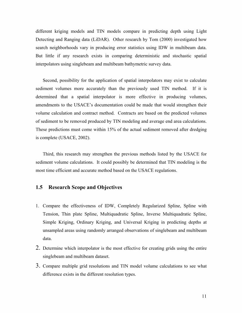
Second, possibility for the application of spatial interpolators may exist to calculate
sediment volumes more accurately than the previously used TIN method. If it is
determined that a spatial interpolator is more effective in producing volumes,
amendments to the USACE’s documentation could be made that would strengthen their
volume calculation and contract method. Contracts are based on the predicted volumes
of sediment to be removed produced by TIN modeling and average end area calculations.
These predictions must come within 15% of the actual sediment removed after dredging
is complete (USACE, 2002).
Third, this research may strengthen the previous methods listed by the USACE for
sediment volume calculations. It could possibly be determined that TIN modeling is the
most time efficient and accurate method based on the USACE regulations.
1.5 Research Scope and Objectives
1. Compare the effectiveness of IDW, Completely Regularized Spline, Spline with
Tension, Thin plate Spline, Multiquadratic Spline, Inverse Multiquadratic Spline,
Simple Kriging, Ordinary Kriging, and Universal Kriging in predicting depths at
unsampled areas using randomly arranged observations of singlebeam and multibeam
data.
2. Determine which interpolator is the most effective for creating grids using the entire
singlebeam and multibeam dataset. 3. Compare multiple grid resolutions and TIN model volume calculations to see what
difference exists in the different resolution types.

12
4. Calculate sediment accretion rates for the Atlantic Ocean Channel to determine at
what rate the channel sea floor is shoaling
1.6 Organization of this Thesis
This thesis is organized into six main chapters. Chapter one includes a problem
statement, project site description and an overview of the spatial interpolators that are
used in this research. The second chapter includes a literature review on previous
Atlantic Ocean Channel studies, a detailed description of the spatial interpolators used in
this research, prior research using spatial interpolation and hydrographic survey data and
the USACE regulations regarding sediment volume estimation. Chapter three gives a
complete methodology description that includes data acquisition and preparation. This
chapter also discusses initial interpolation testing along with a sensitivity analysis
description. The fourth chapter gives results of the initial testing, the sensitivity analysis,
and the descriptive and analytical statistics comparing and contrasting each dataset
evaluation. Chapter five is a discussion of the results from the volume, grid and TIN
analysis. Chapter six provides a conclusion that discusses the decision process of
choosing the most effective interpolator and also a comparison of the volume calculation
methods. Also included in chapter six are recommendations for further research in this
field.

13
2 Literature Review 2.1 Overview
Discussed in this chapter are previous Atlantic Ocean channel studies for
determining shoaling rates. A discussion of hydrographic survey data is included
supported by USACE collection methodology and accuracy standards. Also discussed
are the spatial interpolation methods used in this research and USACE methods in
producing sediment volume estimates.
2.2 Previous Atlantic Ocean Channel Studies
The Atlantic Ocean Channel was formed in 1985 in response to the Norfolk
Harbor Channel and Deepening project. It serves as the main channel that leads all major
shipping traffic into the Chesapeake Bay. Ships exit the Atlantic Ocean channel and then
take course to the Thimble Shoal Channel in route to Norfolk, Virginia or Cape Henry
Channel in route to Baltimore, Maryland or other destinations north.
A deepening study was conducted in 1985 when the Atlantic Ocean channel was
being formed (Berger, Heltzel, Athow, Richards, & Trawle, 1985). USACE scientists
needed to determine at what rate the channel would shoal or deepen at its planned
location. The report used analytical and empirical formulas to predict shoaling rates
caused by tide and wave induced sediment movement. The report also included analysis
of old bathymetric surveys.
It was concluded in this study that the Atlantic Ocean channel would shoal at a
rate of 200,000 cubic yards annually. Other conclusions stated that tidal and wave effects
only produced minimal shoaling effects. The strongest conclusion made in the study was
the comparison of bathymetric surveys. It was stated that long term scour was present
and that the channel was relatively stable (Berger, Heltzel, Athow, Richards, & Trawle,

14
1986).
2.3 Hydrographic Survey Techniques
Guidelines and specifications for creating bathymetric surveys are listed in a
document produced by the USACE known as the “Engineering and Design Hydrographic
Surveying.” Within this document is a full description of survey collection methodology,
survey planning, sediment volume estimation, accuracy standards and design engineering
concepts. This document, last published in 2002, was created to insure consistency of all
survey projects maintained by the USACE.
Hydrographic surveying is performed to determine the underwater characteristics
of a project site. In this application, the underwater topography of a navigation channel is
needed. Surveys are critical to the planning and design of a channel and are extremely
critical to the payment for sediment removal (USACE, 2002). Survey projects of all
types exist that include: payment surveys, plans and specifications surveys, before and
after dredging surveys, project condition surveys, river stabilization, underwater
obstruction, coastal engineering and wetland surveys. Each survey type has a specific
duty that aids in the planning and implementation of sediment removal, shoreline
stabilization, or sediment calculations. Price estimates for contracts that are awarded to
projects are based from surveys.
A hydrographic survey is essentially a topographic map of an underwater surface
(USACE, 2002). The USACE collects data with the same methodology as most
construction and survey companies. Surveys are essentially locations taken in a three
dimensional space as X-Y-Z points. Cross-sections of navigation channels are taken in
the same manner as for highway construction. The surveys are parallel transects that run
perpendicular to the channel or highway direction (USACE, 2002). Locations of survey
points are recorded using a differential GPS aboard a survey vessel. All survey data are
stored electronically in a digital terrain-mapping format.
15
The main characteristic that separates hydrographic surveys from land surveys is
the datum. Land surveys can readily reference coordinates to a datum because land is a
surface that maintains a constant datum. Water levels change two to four times a day,
requiring correction to achieve a constant survey plane. The survey plane in
hydrographic mapping applications is the water’s surface. To achieve a water surface
datum, the water survey plane must be referenced to a known ground point. Surveys are
corrected with tidal factors and adjusted to provide depths at lower low mean water
depth. These factors are produced by the National Ocean Service (USACE, 2000). Error
and uncertainty are key components in fully addressing a survey’s accuracy. Error
causing components consist of the following: Measurement method (acoustic or manual),
sea state, water temperature, salinity, transducer beam width, bottom irregularity, and
heave-pitch-roll motions (USACE, 2002).
Vertical and horizontal accuracy must be addressed to properly record a depth at a
known point. Overall accuracy is dependent on physical conditions along with
systematic and random errors that are associated with hydrographic surveying. Because
of this, comparing survey points at the same location from each year to the next is subject
to inaccuracy and criticism (USACE, 2002). Error is measured in a three – dimensional
ellipsoid, which can be seen below in figure 2.3-1. Most error found in hydrographic
surveys is in the X, Y plane due to more accurate depth recording equipment in
comparison to the differential GPS recorders used. The total allowable error for
singlebeam and multibeam surveys used in this research is +/- 0.9 – 2.0 feet. This error
tolerance is standard for coastal and offshore channels with a tide range of 4 – 8 feet
(USACE, 2002).

16
Figure 2. 3-1 Three-dimensional uncertainty of a measured depth (USACE, 2002)
2.4 Interpolation
2.4.1 Overview
Section 2.4 includes a discussion of all the spatial interpolation methods used in
this research. Spatial interpolation is used to determine phenomena over a continuous
space. In this application, spatial interpolation is used to convert point data of depth
recordings into continuous surfaces. These surfaces will be later used to determine
sediment volume levels. The first form of spatial interpolation consisted of contour
mapping, a two - dimensional representation of a three – dimensional surface (Collins,
1995, Lam, 1983). Spatial interpolators differ in methodology, perspective (assume local
or global influence) and their deterministic or stochastic nature. Deterministic
interpolators provide error measurements produced by testing known point values
through cross validation and validation. Stochastic interpolators produce error statistics
on estimated values produced in the interpolation process. Stochastic interpolator error

17
statistics forecast possible error that will be produced in the interpolation process
(Collins, 1995). The performance of each interpolator will depend on the arrangement,
density and variability of the point data. According to Collins (1995), the choice of
spatial interpolation depends on the following:
1) The planimetric (x, y) and the topographic (z) accuracy of the data;
2) The spatial arrangement and density of the data;
3) Prior knowledge of the surface to be interpolated;
4) Accuracy requirements of the surface being interpolated; and
5) Computation and time limitations to calculate each surface.
If data measurement error is not addressed or if the data is insufficiently sampled,
differences between interpolation techniques would be unjustifiable. Data density and
observational error play the largest role in spatial interpolation performance (Collins,
1995). All of the equations listed in this chapter are from the Using ArcGIS
Geostatistical Analyst book. Geostatistical Analyst is an ArcGIS 8.2 extension used in
this research to perform all interpolation testing.
2.4.2 Inverse Distance Weighting
Inverse distance weighting (IDW) is a deterministic interpolation method in
which values at unsampled points are calculated from known points using a weight
function in a search neighborhood. Known values are used to determine unknown values
surrounding each data point. With this in mind, points closer to the predicted area have
more influence than points of further distance (Johnston, Ver Hoef, Krivoruchko and
Lucas, 2001). IDW is one of the simpler interpolation techniques in that it does not
require pre-modeling like kriging (Tomczak, 1998). The formula and the weighting
function used for IDW can be seen in the equations listed below.

18
The formula used for IDW is as follows:
∑=
=N
iSZ
10
^)( λ iZ(Si)
Where:
)( 0
^SZ is the value to be predicted for location s0.
N is the of sampled points surrounding the prediction location
tλ are the weights assigned to each measured point. These weights decrease with
distance.
Z (si) is the observed value at the location si.
The formula used to determine weights for known values is:
∑=
−−=N
i
p
io
p
ioi dd1
/λ 11
=∑=
N
iiλ
As the distance increases, the weight is reduced by a factor of p.
The quantity di0 is the distance between the predicted location, s0, and each of the
measured locations, si.
The power function used in this thesis automatically sets itself by using a sample
of neighborhood search points. Using this sample, weights are adjusted to produce the
lowest root mean square predicted error from the sample search points.
IDW is an exact interpolator that produces surfaces similar to a bull’s eye shape.
Because more influence is put on known observations closest to the predicted point,
circular rings are present (Tomczak, 1998, and Collins, 1995). This visual effect is more
obvious when interpolating sparse datasets over a large spatial extent.
2.4.3 Splines Splines, also known as radial basis functions (RBFs), are deterministic
interpolators that attempt to fit a surface through each observation of a dataset while also

19
minimizing the total curvature of a surface (Johnston, Ver Hoef, Krivoruchko and Lucas,
2001, Cressie, 1993, Davis, 1986, Collins, 1995). Splines are well suited for calculating
surfaces from a large set of data points that have a gently sloping surface like elevation,
or in this application, sea floor depths. Splines are inappropriate for producing surfaces
from datasets that are prone to error and also datasets with large or rapid changes in the
surface values. Splines were popular in the 1970’s and 1980’s because they were
computationally efficient (Collins, 1995).
Spline functions force the surface to pass through each point but do not provide
estimate of error like most kriging methods (Cressie, 1993). Splines are also very
effective for producing surfaces from regularly spaced data. Unlike IDW, splines can
estimate surface values above and below the maximum and minimum values. Splines
follow a curvature that is produced by the values of the observations. IDW does not
produce values higher than the maximum value because influence on observations
decrease with distance from a known point, thus creating a bull’s eye effect. Splines
calculate surfaces by producing weighted averages of neighboring locations while
passing through known locations (Johnston, Ver Hoef, Krivoruchko and Lucas, 2001).
Five different spline functions (Completely Regularized Spline, Spline with
Tension, Multiquadratic Spline, Inverse Multiquadratic Spline, and Thin Plate Spline)
were used in this thesis. Though little difference exists among spline equations, each was
tested because of spline function’s documented success using large, uniform datasets like
the hydrographic surveys present in this research. A smoothing parameter is used to
determine the smoothness of the calculated surface. With the exception of inverse
multiquadratic spline, the higher the parameter, the smoother the surface. The smoothing
parameter function σ is found by minimizing the root-mean-square prediction errors
using cross-validation (Johnston, Ver Hoef, Krivoruchko and Lucas, 2001).
The spline functions used in this research and a description of parameter
calculation are listed below:

20
Completely Regularized Spline function:
E
nn
nCrEr
nnrr ++=
−−= ∑
∞
=
21
22
1)2/*()2/*ln(
!)*()1()( σσ
σφ
Where ln is the natural logarithm, E1(x) is the exponential integral
function, and CE is the Euler constant.
Spline With Tension function:
ECrKrr ++= )*()2/*ln()( 0 σσφ
Where K0(x) is the modified Bessel Function
Multiquadratic Spline function:
2/122 )()( σφ += rr
Inverse Multiquadratic Spline function:
2/122 )()( −+= σφ rr
Thin-Plate Spline function:
)*ln()*()( 2 rrr σσφ =
2.4.4 Kriging Kriging is synonymous with “optimal prediction” as kriging attempts to make
inferences on unobserved values (Cressie, 1993). Kriging is a stochastic technique that
uses a linear combination of weights at known points to estimate the value at an unknown
point (Collins, 1995). Kriging builds these inferences and estimates using a
semivariogram, a measure of spatial correlation between two points. Weights are given
to points that have similar directional influence and distance. A semivariogram bases
these predictions by the level of spatial autocorrelation, that is, dependence between
sample data values which decrease as the distance between observations increase (Lam,

21
1983).
Kriging was invented by the aid of a South African mining engineer named D.G.
Krige. Krige used empirical observations of weighting to estimate the ore content of
mined rock by comparing known values sampled from early mining explorations
(Cressie, 1993, Collins, 1995, Lam, 1983). Later, G. Matheron, a Frenchman,
incorporated Krige’s methodology into a technique he dubbed as “Kriging”, the theory of
the behavior of spatially distributed variables (Collins, 1995).
The semivariogram is used in kriging to develop a prediction of the expected
difference in values between pairs of data with similar orientation (Collins, 1995, Lam,
1983). The semivariogram is a representation of the average rate of change of a property
with distance. Figure 2.4.3-1 shows a simple variogram.
Figure 2.4.4-1 Semivariogram
Nugget: Variance of unresolved predictions (noise)
Sill: Maximum variance
Range: Distance after which correlation is zero

22
The equation used to calculate the semivariogram ( r ) is defined by:
∑=
−+=N
iii xzdxzNr
1
2)]()([2/1
Where d is the distance between two samples (Lam, 1983). The semivariogram
represents the relationship between half the mean square difference between sample
values and their intervening distance.
Computation of a semivariogram model begins by creating an experimental
variogram using a sample of available data. The semivariogram provides all the
information needed about a regionalized variable, including the size of the zone of
influence around a sample, the isotropic or anisotropic nature of the variable, and the
consistency of the variable through space (Cressie, 1993, Collins, 1995). Kriging faces
much criticism due to visual fitting of semivariogram to data, but aside from
semivariogram fitting, it is computationally similar to many spline techniques.
Documented comparison of splines and kriging can be found in literature written by
Cressie (1993).
2.5 Validation and Cross Validation
Since field validation and verification of the accuracy of predicted depths
produced by interpolation in unsampled areas is unattainable, comparison methodology
techniques were used. The goal of this comparative effort is to determine which
interpolator produces the most accurate depths in unmapped areas from these dense
datasets. Each interpolation technique is compared on the basis of mean prediction
error, root mean square error, and total average error. Several sampling methods were
used to determine how each interpolator performed when data was withheld.
Cross validation and validation are two of the most popular methods for
determining spatial interpolator accuracy. Cressie (1993) describes cross validation as a
popular means of assessing statistical estimation and prediction. Cressie (1993) defines
cross validation as deleting parts of data and interpolate using the remaining dataset.

23
Repeating cross validation over many deleted subsets allows an assessment of the
variability of prediction error (Cressie, 1993 and Johnston, Ver Hoef, Krivoruchko and
Lucas, 2001). Cross validation removes one data point from a sample and the remaining
n – 1 observations are used to predict the missing data point. Figure 2.5-1 is an example
of how cross validation removes one point (highlighted in yellow) from the entire dataset
and uses the remainder of the population to interpolate a surface. The measured value is
compared to the predicted value. This procedure is done for the entire population.
Figure 2.5-1 cross validation point removal
Cross validation is extremely effective when using randomly arranged, sparse
datasets. In this application one point from approximately 17,000 points was removed
and the remainder were used to predict. A more effective approach would be to subset
twenty percent of the entire hydrographic survey and use those points (approximately
3,500) to predict depth values. This way, a prediction surface using only twenty percent
of the entire dataset and the entire dataset can be compared for both singlebeam
hydrographic survey data and multibeam hydrographic survey data.
Validation uses a test and training dataset to predict depth values. Validation
operates under the premise that an entire set of data is removed to predict depths.
Therefore, using singlebeam hydrographic survey, approximately 3,500 points are
removed and used as a training dataset. The remaining 14,000 points, known as the test
dataset, are used to predict the 3,500 removed points. From this, mean prediction errors
(MPE) and root mean square errors (RMSE) are produced (Ver Hoef, Krivoruchko and
Lucas, 2001). The interpolation technique that produces the lowest total average error,
which is a combination of RMSE and MPE, will produce the most accurate portrayal of

24
channel depths.
2.6 Previous Research using Hydrographic Survey Data
The majority of work completed in the field of hydrographic surveying involves
addressing survey uncertainty and limited spatial interpolation investigation. Most
research available today deals with the application of spatial interpolation using
meteorological and soil data. Collins (1995) cites over twenty different research articles
and books that address comparative research of spatial interpolation when applied to soil
and precipitation. There are few documented sources comparing spatial interpolation
methods when using hydrographic data.
Johnston (2002) created bathymetric surfaces by using TIN modeling and five
different kriging model methods. This research used SHOALS (USACE LiDAR) to
determine which kriging-weighting model produced the lowest amount of error. The
kriging models used in this research were as follows: linear, spherical, exponential,
Gaussian, and circular weighting schemes. Johnston determined with 95% confidence
that neither of the weighting schemes produced prediction error above 15 centimeters, the
USACE error standards for SHOALS. Johnston also compared the depths of the kriging-
derived surfaces to TIN models. TIN models were converted to grids of varying
resolution and each depth was compared on cell – by –cell basis. Johnston concluded
that depth readings of kriging derived grids and TIN derived grids of varying resolutions
did not vary in uncertainty, but indicated to use TIN modeling because it does not
inherently smooth data like kriging.
Tom (2000) investigated building surfaces from varying search neighborhood
types using IDW applied to multibeam survey data. Tom used a local linear interpolator
such as inverse distance weighting and compared several search neighborhood
techniques. The search neighborhoods used were a simple, a quadrant and an octant. A
simple search only uses the nearest data points from the center of the search circle. A
quadrant evenly assigns the same number of observations to four different quadrants. An

25
octant divides the same number of points from the simple search in eight different
quadrants. Tom concluded that the four-quadrant neighborhood estimates with the lowest
RMSE using varying data density regardless of the power function. Tom also concluded
that using a higher or optimally calculated power function also produces lower RMSE.
2.7 Shoaling
The most common forms of shoaling that the Atlantic Ocean channel experiences
are regional siltation and side slope failure (Pope, 2002). Regional siltation is a product
of fine-grained sediment from storm watershed runoff or from offshore sources.
Sediment found in river and bay/estuary channels generally comes from watershed runoff
in upland areas. Offshore sediments are generally carried by storm surge or abnormally
strong tides and are coarser in deep ocean channels. This sediment is usually in
suspension at ocean inlet channels (Pope, 2002).
Geotechnical shoaling or side slope failure is another common form of shoaling
found more often in bay channels than ocean channels. Side slope failure is caused when
a major dredging project has occurred. The side slopes have been distinctly scoured and
sediment from the sidewalls of the channel creep with the aid of tide and sea floor
currents (Pope, 2002). The channel shoals at the extreme left and right sides but
increases its width, which helps to aid in navigation. Over time, the entire channel will
begin to shoal and dredging must be implemented again (see figure 2.7-1).

26
Figure 2.7-1 Cross Sectional and Planform View of regional siltation and
geotechnical slope failure.
The Atlantic Ocean Channel is a deep-water channel that has not experienced
dredging to aid in deepening for safe passage. Once this channel is dredged, it will be
susceptible to geotechnical slope failure, a common type of shoaling that is present in bay
channels that experience maintenance dredging.
2.8 Volume Estimation
The USACE produce sediment volumes very similar to most highway design
engineering by using an average end area calculation (AEA). Cross sections of a channel
are taken at a constant interval and the quantity is computed on the basis of volume
between the cross sections (USACE, 2002). AEA is used when cross section spacing is

27
large and there are not enough sample survey points to produce an accurate grid. The
cross sectional method of AEA uses a horizontal projection to calculate sediment.
Because it does not produce a continuous surface like a TIN, it uses distance and the sum
of each volume divided by 0.5 to produce volumes. The calculation used horizontal AEA
can be seen in figure 2.8-1.
Figure 2.8-1 Horizontal Average End Area diagram (USACE, 2002)
V = 0.5(A1+A2)*D
Where: V is the volume A1 is the first area of the cross section A2 is the second area of the cross section D is the distance between cross sections.

28
TIN models are also used in the AEA calculation to produce volume of sediment.
TINs are used for sparse cross section data (USACE, 2002). They produce sediment
volume on a vertical projection because they are continuos surfaces in which vertical
heights above the plan form of the channel can be measured. Bin modeling is another
method the USACE implements in producing volumes. Bins are grid layers created from
dense multibeam data that estimate volume on a cell – by – cell basis (USACE, 2002).
The illustration and equations used for TIN and Bin vertical AEA can be seen in figure
2.8-2.
Figure 2.8-2 Vertical Projection for average end area calculations (USACE, 2002)
Where: h1, h2, h3 = the height of each triangle above the reference surface
Ao = the area of the reference plane triangle
hb = the height of the grid above the reference surface
Ab = the depth of the reference surface
Vertical Projection (Grid/Bin) Volume of element: V = hb* Ab
Vertical Projection (TIN) Volume of element: V=1/3 (h1+h2+h3) * A0

29
3 Methodology 3.1 Overview
Chapters 1 and 2 provided insight to the defined problem and the interpolation
methods used in this thesis. This chapter provides the research methodology used in the
comparative analysis of spatial interpolation. The process of data gathering, data
preparation, interpolation, comparison analysis, and sensitivity analysis will be addressed
in detail. A discussion of volume analysis and grid creation is also included. Also
mentioned in this chapter are the different software packages used for data preparation
and analysis.
3.2 Data Gathering and Preparation
The analysis of this thesis used singlebeam and multibeam hydrographic survey
data collected by the USACE, Norfolk, VA District. The USACE, Norfolk began
archiving digital survey records in 1988 but did not record the first digital Atlantic Ocean
Channel survey until October 1994. Prior bathymetric surveys were taken in mid to late
1980’s but were unattainable in digital format. A soil and geologic survey was taken in
March 1986, which included depth estimates and sediment description of 86 sediment
samples taken throughout the channel (USACE, 1986).
The USACE produce multiple survey types for varying project types. This list of
survey types include: dredging measurement and payment surveys, plans and
specification surveys, before and after dredging surveys, project condition surveys,
elapsed time between condition surveys, river stabilization project surveys, underwater
construction or condition surveys, coastal engineering surveys, reservoir sediment
surveys, inland navigation charting surveys, wetland surveys, and miscellaneous surveys
(USACE, 2002).
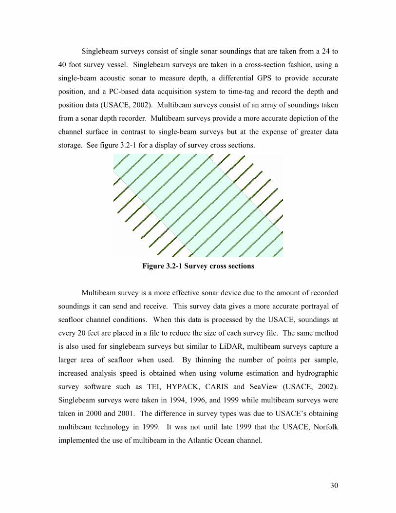
30
Singlebeam surveys consist of single sonar soundings that are taken from a 24 to
40 foot survey vessel. Singlebeam surveys are taken in a cross-section fashion, using a
single-beam acoustic sonar to measure depth, a differential GPS to provide accurate
position, and a PC-based data acquisition system to time-tag and record the depth and
position data (USACE, 2002). Multibeam surveys consist of an array of soundings taken
from a sonar depth recorder. Multibeam surveys provide a more accurate depiction of the
channel surface in contrast to single-beam surveys but at the expense of greater data
storage. See figure 3.2-1 for a display of survey cross sections.
Figure 3.2-1 Survey cross sections
Multibeam survey is a more effective sonar device due to the amount of recorded
soundings it can send and receive. This survey data gives a more accurate portrayal of
seafloor channel conditions. When this data is processed by the USACE, soundings at
every 20 feet are placed in a file to reduce the size of each survey file. The same method
is also used for singlebeam surveys but similar to LiDAR, multibeam surveys capture a
larger area of seafloor when used. By thinning the number of points per sample,
increased analysis speed is obtained when using volume estimation and hydrographic
survey software such as TEI, HYPACK, CARIS and SeaView (USACE, 2002).
Singlebeam surveys were taken in 1994, 1996, and 1999 while multibeam surveys were
taken in 2000 and 2001. The difference in survey types was due to USACE’s obtaining
multibeam technology in 1999. It was not until late 1999 that the USACE, Norfolk
implemented the use of multibeam in the Atlantic Ocean channel.

31
All surveys were stored in .DTM (digital terrain model) format, which was later
post processed by the USACE for use. Each survey is adjusted to give readings at mean
lower low water levels to stay consistent (USACE, 2002). The National Ocean Service
determines mean lower low water by calculating time delay in tide conditions and water
slope correction factors using a Tidal Zoning Plan. Mean lower low water is 1.3 feet
below the National Geodetic Vertical Datum (NGVD), 1972 adjustment. This measure
was determined at the Chesapeake Bay Bridge Tunnel (USACE, 2000, USACE, 2002).
After each archived survey was found for the Atlantic Ocean Channel, it was
converted from the .DTM format to a .TXT (text file) format by using Navigation
Support, software created by the USACE, Norfolk District. Because survey data is
streaming or continuous in form, it is filtered to show soundings at every twenty feet.
Navigation Support is used to identify areas of shoaling and the relationship to
environmental channel form and the plan form. The environmental channel form is the
actual sea floor shape portrayed in a cross-sectional view (see figure 3.2-2). Once in
.TXT format, survey information such as date recorded and survey stations recorded
could be viewed.
After each survey was converted to .TXT format, it was then opened in Microsoft
Excel and saved as a .CSV (comma delimited) file. The file consisted of X & Y
coordinates and also contained a positive Z value (depth). This depth field (Z) was later
converted to a negative number for interpolation and volume calculations by multiplying
the Z values by -1. Each survey was collected and recorded by the USACE, Norfolk in
Stateplane, NAD 27 coordinate system. These files were then exported to a shapefile
(.shp) format for GIS analysis. Each survey from 1994 – 2001 contained four survey
segments for the Atlantic Ocean Channel that required merging. File merging was
performed using Arcview 3.2 Geoprocessing wizard. The data density for each survey is
listed in table 3.2-1.
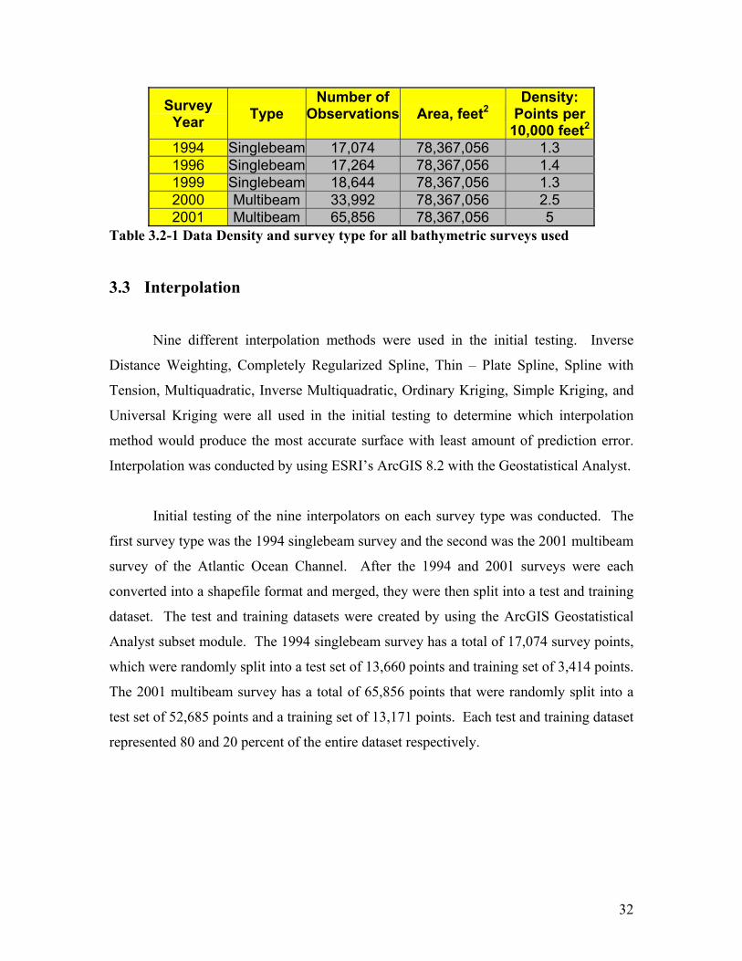
32
Survey Year Type
Number of Observations
Area, feet2
Density: Points per
10,000 feet2
1994 Singlebeam 17,074 78,367,056 1.3 1996 Singlebeam 17,264 78,367,056 1.4 1999 Singlebeam 18,644 78,367,056 1.3 2000 Multibeam 33,992 78,367,056 2.5 2001 Multibeam 65,856 78,367,056 5
Table 3.2-1 Data Density and survey type for all bathymetric surveys used
3.3 Interpolation
Nine different interpolation methods were used in the initial testing. Inverse
Distance Weighting, Completely Regularized Spline, Thin – Plate Spline, Spline with
Tension, Multiquadratic, Inverse Multiquadratic, Ordinary Kriging, Simple Kriging, and
Universal Kriging were all used in the initial testing to determine which interpolation
method would produce the most accurate surface with least amount of prediction error.
Interpolation was conducted by using ESRI’s ArcGIS 8.2 with the Geostatistical Analyst.
Initial testing of the nine interpolators on each survey type was conducted. The
first survey type was the 1994 singlebeam survey and the second was the 2001 multibeam
survey of the Atlantic Ocean Channel. After the 1994 and 2001 surveys were each
converted into a shapefile format and merged, they were then split into a test and training
dataset. The test and training datasets were created by using the ArcGIS Geostatistical
Analyst subset module. The 1994 singlebeam survey has a total of 17,074 survey points,
which were randomly split into a test set of 13,660 points and training set of 3,414 points.
The 2001 multibeam survey has a total of 65,856 points that were randomly split into a
test set of 52,685 points and a training set of 13,171 points. Each test and training dataset
represented 80 and 20 percent of the entire dataset respectively.
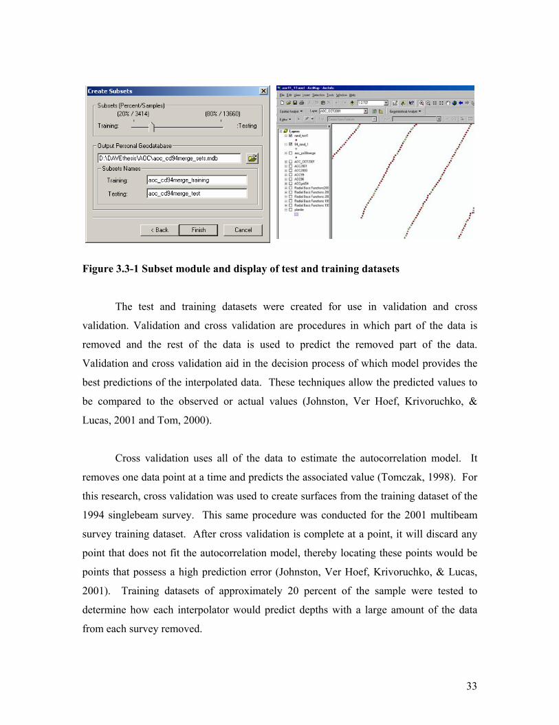
33
Figure 3.3-1 Subset module and display of test and training datasets
The test and training datasets were created for use in validation and cross
validation. Validation and cross validation are procedures in which part of the data is
removed and the rest of the data is used to predict the removed part of the data.
Validation and cross validation aid in the decision process of which model provides the
best predictions of the interpolated data. These techniques allow the predicted values to
be compared to the observed or actual values (Johnston, Ver Hoef, Krivoruchko, &
Lucas, 2001 and Tom, 2000).
Cross validation uses all of the data to estimate the autocorrelation model. It
removes one data point at a time and predicts the associated value (Tomczak, 1998). For
this research, cross validation was used to create surfaces from the training dataset of the
1994 singlebeam survey. This same procedure was conducted for the 2001 multibeam
survey training dataset. After cross validation is complete at a point, it will discard any
point that does not fit the autocorrelation model, thereby locating these points would be
points that possess a high prediction error (Johnston, Ver Hoef, Krivoruchko, & Lucas,
2001). Training datasets of approximately 20 percent of the sample were tested to
determine how each interpolator would predict depths with a large amount of the data
from each survey removed.

34
Validation uses a test and training dataset for calculating prediction error (Tom,
2000). In this research, a training dataset of 3,414 points were randomly selected and a
test dataset of 13,660 points were also selected for the 1994 singlebeam survey. For the
multibeam survey 13,171 points were used for the training dataset and 52,685 points
were used for the test dataset. Each dataset was 20 and 80 percent of the total dataset,
respectively. Validation creates a model only for a subset of the total data. It compares
the removed data (test dataset) to the observed data at one time. The training dataset is
used to calculate or predict the actual values of the test dataset (Johnston, Ver Hoef,
Krivoruchko, & Lucas, 2001).
3.4 Prediction Error Gathering
ArcGIS Geostatistical Analyst used training and test data sets to calculate
validation statistics for each interpolation method and examined the entire data set to
produce validation statistics for each interpolation method. Cross – validation was
performed on 20 percent of the observations to determine which interpolation technique
performed the best when data is withheld. Each interpolation method was tested and the
mean prediction error (MPE) and root mean square error (RMSE) of validation and cross
validation were collected.
Using the RMSE and mean prediction error from validation and cross –
validation, each value was assumed as an absolute value and recorded. The RMSE and
mean prediction error were used in this analysis because these values were the only two
error values that were produced in every interpolation technique. All of the kriging
methods produced average standard error, mean standardized prediction error, and RMSE
standardized prediction error because they are stochastic interpolation methods. Kriging
methods use empirical semivariogram and covariance functions to estimate kriging
predictors and standard errors, values that are not produced by deterministic interpolation
methods (Johnston, Ver Hoef, Krivoruchko, & Lucas, 2001, Johnston, 2002).

35
3.5 Interpolation Methods – Initial Testing
This section discusses the methodology used in initial interpolation of singlebeam
and multibeam data. A cross validation dataset and validation dataset were used for all
interpolation methods. A four-quadrant search model and a search center point
coordinate of X: 2769327.2 and Y: 206414.83 was used in the model setup of each
interpolator. The four-quadrant model was used to calculate parameters such as optimal
weight distance for IDW, parameter weighting for splines, and semivariogram/
covariance modeling for kriging. Universal kriging also used the setup model for
detrending data using a local or global polynomial weighting function. Each parameter
or weight is determined by calculating RMSE from a sample of points. Error statistics
(MPE and RMSE) are recorded and combined into a total average for ranking of
interpolators. The average total error consists of the mean prediction error and the RMSE
calculated in cross validation and validation. Each validation and cross validation MPE
and RMSE error value from each dataset is added and divided by 4 to create the average
total error. A total of 18 grids were created in this portion of the analysis.
3.5.1 Inverse Distance Weighting (IDW)
Using ArcGIS Geostatistical Analyst, the 1994 singlebeam and 2001 multibeam
surveys were used to create a temporary grid surface by the IDW technique. The search
power was optimized and 200 neighbors were selected using a circular, four-sector search
method. Tom (2000) concluded that a four-sector search produced the lowest sampling
RMSE when creating a surface. Validation and cross – validation MPE and RMSE and
temporary surfaces were produced and recorded. Figures 3.5.1-1 and 3.5.1-2 are a
graphical display of the interface used in this analysis. Each of the figures provides the
initial selection of datasets and the search model setup respectively.

36
Figure 3.5.1-1 Geostatistical Analyst interface for IDW
Figure 3.5.1-2 IDW setup model for calculating optimal weight

37
3.5.2 Spline – Completely Regularized, Tension, Multiquadratic, Inverse Multiquadratic & Thin – Plate
Spline techniques followed similar methodology to IDW except that only 16
neighbors could be selected using the Geostatistical Analyst. Splines are fast
interpolators but optimally calculating the parameter function is time consuming process.
Parameters are calculated to “smooth” an interpolated surface. The parameter function is
calculated by using the 64 neighbors (4 X 15) in the setup parameter interface (see figure
3.5.2-1). With exception of inverse multiquadratic spline, the higher the parameter, the
smoother the surface. The singlebeam and multibeam survey data were used in
validation and cross validation and error statistics were recorded.
Figure 3.5.2-1 Parameter optimizing feature
3.5.3 Kriging – Ordinary, Simple, and Universal
Kriging techniques involved more steps than the IDW and spline interpolators.
Semivariogram modeling is incorporated into the interpolator to measure the level of
spatial autocorrelation. Autocorrelation is the statistical comparison between spatial
random variables of the same type or attribute in which correlation depends on the
distance and /or direction that separates the locations (Johnston, Ver Hoef, Krivoruchko,
and Lucas, 2001, Cressie, 1993, and Davis, 1986). The attribute measured in this
research is depth.
The first step is to select the prediction map option, which will create a grid
surface of depth values. Kriging can also develop surfaces that describe the prediction
standard error and probability of the data that is interpolated. The second step is to model
the semivariogram. Semivariogram fitting can be an extremely crucial step in modeling
randomly arranged data, but for this research, most search models are acceptable.
According to Johnston (2002) the search model does not effect semivariogram building
when using highly populated datasets such as LiDAR, multibeam and singlebeam

38
hydrographic data. For this research, a spherical curve fitting for the semivariogram was
used. Universal kriging implemented a detrending process, which based its
semivariogram model from a global or local polynomial function. A 100% local
polynomial function was used in this research because of the highly populated and dense
datasets
Figure 3.5.3-1 Semivariogram building
Range, nugget, and sill values are automatically calibrated by examining the
search neighborhood sample point’s RMSE. Semivariogram/covariance surface creation
was calibrated by implementing search direction parallel to the channel direction. The
search direction aids in semivariogram building by determining if anisotropy exists in the
data. The search direction function is highlighted in red. The listed angle direction,
angle tolerance and bandwidth (lags) are user specified. The values seen above were
used in this research and are as follows: Angle direction, 309, Angle Tolerance, 42.0, and
Bandwidth (lags), 3.6. These values were used due to the anisotropic nature of the data

39
that encompasses a majority of the range (indicated in blue) and the less correlated data
highlighted in red and orange.
The third step of the kriging analysis is to create a search neighborhood of sample
points. For kriging, this step is useful if the researcher knows where anisotropy in the
data exists. For this research, anisotropy is not assumed or known, therefore the previous
X, Y coordinates were used to maintain consistency in the research. Once the
semivariogram model is fit, cross validation and validation statistics are calculated and
recorded.
Figure 3.5.3-2 Kriging search neighborhood
Cross validation and validation statistics were collected for each interpolator. These
statistics were calculated using the Geostatistical Analyst extension from ArcGIS 8.2.
The figures listed below provide a visual display of the regression plot comparing known

40
versus predicted values. The mean prediction error and RMSE scores were recorded and
tabulated for further analysis.
Ranking of interpolators was conducted by averaging cross validation and validation
MPE and RMSE scores. The four interpolators that produce the lowest mean total error
will be later used in the sensitivity analysis of singlebeam and multibeam hydrographic
surveys.
Equation for calculating Mean Total Error
ValMPE1 + ValRMSE1 + CValMPE2 + CValRMSE2 = Mean Total Error
3.6 Interpolation Testing – Sensitivity Analysis
Three sensitivity analyses were performed in this research. The interpolation
methods to produce surfaces in this section follow exactly as listed in section 3.5. Cross
validation and validation MPE and RMSE were calculated, combined and averaged to
determine which interpolator produced the lowest mean total error.
3.6.1 Randomly Arranged Samples
The first analysis incorporated the four interpolators that produced the lowest mean
prediction error and RMSE in the initial interpolation testing of both singlebeam and
multibeam hydrographic data. An average of the MPE and RMSE was calculated to
determine which interpolator produced the lowest error. Each interpolator from both
datasets was tested using 10 randomly generated test and training datasets. Each test and
training dataset was created by using Microsoft Excel’s random number generator. The
database file from singlebeam and multibeam surveys was opened and a random number
field was generated. After applying the random number to each cell of the random
number column, a resort of values was conducted to scramble the arrangement of data
points. The corresponding X, Y coordinates remain intact but the order of the
observations is randomly sorted. The first 20% of the data values are saved as a .CSV
and converted to a shapefile as a training set for use in the analysis. The remainder of the

41
values (80%) are also saved as a .CSV and then converted to a shapefile as a test set for
use in the analysis. A total of thirty randomly arranged datasets were created using
singlebeam hydrographic data while ten randomly arranged test and training datasets
were created using multibeam hydrographic survey data. Eighty grids were created in
this portion of the analysis. Cross validation and validation statistics were calculated and
recorded.
Matched pair t-Tests were used to compare the mean total error produced by each
interpolator. This will aid in the decision process of determining what interpolator is the
most effective in producing depths. Using matched pair t-Tests may also indicate that no
difference exists in the mean total error produced, making the choice of optimal
interpolator strictly the preference of the user.
3.6.2 Lowest and Highest Error Producing Interpolators
The second analysis incorporated testing of the highest and lowest error producing
interpolators. A thirty sample testing of random test and training datasets using the
highest error producing interpolator and lowest error producing interpolator was
conducted to determine if a range of mean total error overlap occurred. This analysis was
conducted using singlebeam hydrographic survey data only. Calculation times hindered
the success of this analysis applied towards multibeam hydrographic survey data. Sixty
grids were created in this portion of the analysis. Cross validation and validation
statistics were also recorded and compared for analysis.
3.6.3 Full Cross Validation of Singlebeam and Multibeam data
The third analysis used cross validation of an entire singlebeam and multibeam
hydrographic dataset. This portion of the analysis disregarded the use of test and training
datasets. The main intent was to determine if the optimal interpolator differed from
testing a survey in which data was withheld when an entire dataset was available. These
results aid in the conclusion of choosing an optimal interpolator. A total of 18 grids were
created in this portion of the analysis. Cross validation statistics were recorded and

42
compared to cross validation statistics produced in the initial testing to determine if a
difference in prediction error existed between interpolation of full datasets and
interpolation of randomly arranged datasets when samples are withheld.
Choosing an optimal interpolator will depend on several factors. The first factor is
the how well the interpolator predicts depths at unknown values in the initial
interpolation. The second factor is how well and how consistently each interpolator
predicts depths in the sensitivity analysis. If an interpolator produces low mean
prediction error but has a large range of error, it may not be suitable for further use. The
last but least important component is the computational speed of the interpolator. An
interpolator may produce low and similar prediction error in comparison to another
interpolator but if the computation time is much longer, it may be deemed as inefficient
and unacceptable for use.
3.7 Grid, TIN and Volume Analysis
This section provides detail on the creation of grids and sediment volume estimation
methodology. Grids were created at 15 meters, 30 meters, 60 meters, and 90 meters.
TIN models were also produced in the comparison of volume estimation. A total of 20
grids and 5 TINs were created in this portion of the analysis.
3.7.1 Grid and TIN Construction
After choosing the optimal interpolator for singlebeam and multibeam data, grids
were constructed at four prescribed resolutions for each survey year. Each grid was
clipped using the Atlantic Ocean Channel plan file provided by the USACE, Norfolk and
ARCINFO. The plan file is the polygon that bounds the left and right sides of the
channel’s bottom. The sideslopes of the channel are not included in the plan file.
TINs were created using each survey year provided in this research. Survey depth
observations were used as mass points to construct TIN models. Each TIN was also

43
clipped using the Atlantic Ocean Channel plan file for further use in sediment volume
estimation.
3.7.2 Volume Analysis
Volume estimates were calculated using ArcGIS’s 3D Analyst. After each grid and
TIN had been created, volume estimates were recorded at a plan depth of 53 feet. A plan
depth is used to determine how much sediment is located above that prescribed depth. A
comparison of surveys is deemed inadequate and unreliable because survey points are
rarely located in the same planimetric (X, Y) position. More than likely, estimated or
interpolated values would be compared to determine shoaling which would produce a
large degree of error in the volume estimate. The volumes of each grid resolution and
TINs were then compared to determine if a difference in volume estimates existed
between varying grid resolutions and TIN modeling.

44
4 Results 4.1 Overview
Testing of interpolators on randomly arranged test and training datasets was
performed to measure each interpolator’s effectiveness of predicting depths. The datasets
used for this thesis are systematically taken in linear cross sections but are then randomly
arranged while portions of the data are withheld. Interpolation techniques were compared
by predicting depths using the entire dataset and randomly selected points (test and
training sets) from both singlebeam and multibeam data. The interpolation techniques
are ranked by the average of MPE and RMSE produced by each interpolation method.
Also, the results of the sensitivity analysis are shown to further support the decision
process for selecting the best interpolation technique. Also included in this chapter is a
discussion and analysis of full cross validation. This cross validation technique tests each
interpolator’s ability to interpolate a surface from all of the observations. No randomly
arranged samples are used and all observations are available. Filled depth contour maps
of the full cross validation for both singlebeam data and multibeam data are also
provided.
4.2 Initial Testing
4.2.1 Summary statistics
Using the methodology listed in chapter 3, initial testing was conducted on both
singlebeam and multibeam hydrographic survey data of the Atlantic Ocean Channel.
Summary statistics were produced to gain an overall understanding of depth change
during the seven-year period. Table 4.2.1-1 shows the count, mean, maximum,
minimum, range, variance, and standard deviation of the depth recordings given for both
singlebeam and multibeam data used in this research.

45
Statistic Singlebeam 1994
Singlebeam 1996
Singlebeam 1999
Multibeam 2000
Multibeam 2001
Count 17074 17264 18644 33992 65856 Mean 58.6 56 56.1 55.8 56.2
Maximum 50.9 48.6 49.6 49 49 Minimum 71.9 67.7 68 66.6 68.8
Range 21 19.1 18.4 17.6 19.8 Variance 11.9 13.3 14.6 13.5 18.9 Standard Deviation 3.5 3.6 3.8 3.7 4.3
All values in U.S. feet
Table 4.2.1-1 Summary Statistics of singlebeam and multibeam data
4.2.2 Interpolation Testing
Two initial interpolation testing procedures were used to determine the results of
this research. First, initial testing of all nine interpolators on the 1994 singlebeam survey
data was conducted and second, initial testing of all nine interpolation methods on the
2001 multibeam survey data was conducted. The selected datasets were chosen to
determine interpolation performance and accuracy on the least populated and most
populated datasets. The main purpose of this portion of the analysis is to determine
which interpolator produces the lowest average total error using randomly arranged
observations where portions of the data are withheld. Listed in the performance tables
are mean prediction error (MPE), root mean square error (RMSE), and average total error
for both validation and cross validation techniques. Cross validation was performed on
each dataset using a random 20% of the total population. Validation was performed on
each dataset using a training dataset (20%) and test dataset (80%) of each dataset
population. The training dataset was used to validate the predicted scores produced by
the test dataset. A total of 18 interpolated surfaces were produced in the initial testing.
Also shown are bar graphs to visually support the initial testing results. Tables 4.2.2-1 –
4.2.2-5 show all of the performance statistics produced by each interpolation method. All
values given are in U.S. feet and highlighted values represent interpolators that produced
the lowest error.

46
Interpolator 1994
Singlebeam Survey in Feet
2001 Multibeam Survey in Feet
IDW 0.0215 0.0048 Completely Regularized
Spline 0.0202 0.0015
Spline with Tension 0.0208 0.0012
Multiquadratic Spline 0.0140 0.0010
Inverse Multiquadratic
Spline 0.0435 0.0050
Thin Plate Spline 0.0157 0.0012
Ordinary Kriging 0.0128 0.0016
Simple Kriging 0.0124 0.0017 Universal Kriging 0.0178 0.0208
All values in U.S. feet Table 4.2.2-1 Mean Predicted Error totals in feet of initial interpolation produced from validation of singlebeam and multibeam data.
Listed above in table 4.2.2-1, simple kriging produced the lowest MPE from the
singlebeam dataset and multiquadratic spline produced the lowest MPE from the
multibeam survey dataset. Inverse multiquadratic spline produced the highest MPE from
validation of singlebeam data while universal kriging produced the highest MPE from
validation for multibeam data.
Table 4.2.2-2 displays the validation RMSE produced from both 1994 singlebeam
and 2001 multibeam data. Multiquadratic spline produced the lowest RMSE of 0.7481
feet and 0.2689 feet for both singlebeam and multibeam data. Completely regularized
spline and IDW followed closely behind in producing RMSE values of 0.7492 feet and
0.7517 feet respectively for singlebeam data. Spline with tension and thin plate spline
produced RMSE values of 0.2843 feet and 0.2853 feet respectively using multibeam data.
Universal kriging produced the highest RMSE values for both singlebeam and multibeam
data.

47
Interpolator 1994
Singlebeam Survey
2001 Multibeam Survey
IDW 0.7517 0.4324 Completely
Regularized Spline 0.7492 0.2942
Spline with Tension 0.7572 0.2843 Multiquadratic
Spline 0.7481 0.2689
Inverse Multiquadratic
Spline 1.0720 0.3836
Thin Plate Spline 0.9256 0.2853 Ordinary Kriging 0.7858 0.2916 Simple Kriging 0.7830 0.3044
Universal Kriging 1.3060 0.8728 All values in U.S. feet
Table 4.2.2-2 RMSE values in feet of initial interpolation produced from validation of singlebeam and multibeam data
Cross validation statistics are shown in tables 4.2.2-3 and 4.2.2-4 for both MPE
and RMSE of singlebeam and multibeam data. In table 4.2.2-3, ordinary kriging
produced the lowest MPE score of 0.0013 feet and 0.0001 feet for both singlebeam and
multibeam data respectively. Simple kriging also produced low MPE scores as well for
singlebeam and multibeam data.
Listed in table 4.2.2-4, multiquadratic spline produced the lowest RMSE values of
0.7843 feet and 0.2764 feet for both singlebeam and multibeam data during the cross
validation process. Both spline with tension and completely regularized spline performed
well in producing low RMSE scores for singlebeam and multibeam data. Again,
universal kriging produced the highest MPE and RMSE for cross validation of
singlebeam and multibeam data.

48
Interpolator 1994 Singlebeam Survey in Feet
2001 Multibeam Survey in Feet
IDW 0.0137 0.0062 Completely Regularized
Spline 0.0086 0.0006
Spline with Tension 0.0091 0.0006
Multiquadratic Spline 0.0026 0.0002
Inverse Multiquadratic Spline 0.0316 0.0008
Thin Plate Spline 0.0038 0.0006 Ordinary Kriging 0.0013 0.0001 Simple Kriging 0.0017 0.0002
Universal Kriging 0.0311 0.0227 All values in U.S. feet
Table 4.2.2-3 Mean Predicted Error totals in feet of initial interpolation produced from cross validation of singlebeam and multibeam data
Interpolator 1994 Singlebeam Survey in Feet
2001 Multibeam Survey in Feet
IDW 0.7942 0.4396 Completely Regularized
Spline 0.7860 0.3071
Spline with Tension 0.7930 0.2967
Multiquadratic Spline 0.7843 0.2764
Inverse Multiquadratic Spline 1.0790 0.4644
Thin Plate Spline 0.9553 0.2976 Ordinary Kriging 0.8154 0.2928 Simple Kriging 0.8128 0.3050
Universal Kriging 1.2950 0.8747 All values in U.S. feet
Table 4.2.2-4 RMSE totals in feet of initial interpolation produced from cross validation of singlebeam and multibeam data
The final list of values obtained from the initial interpolation is the combined total
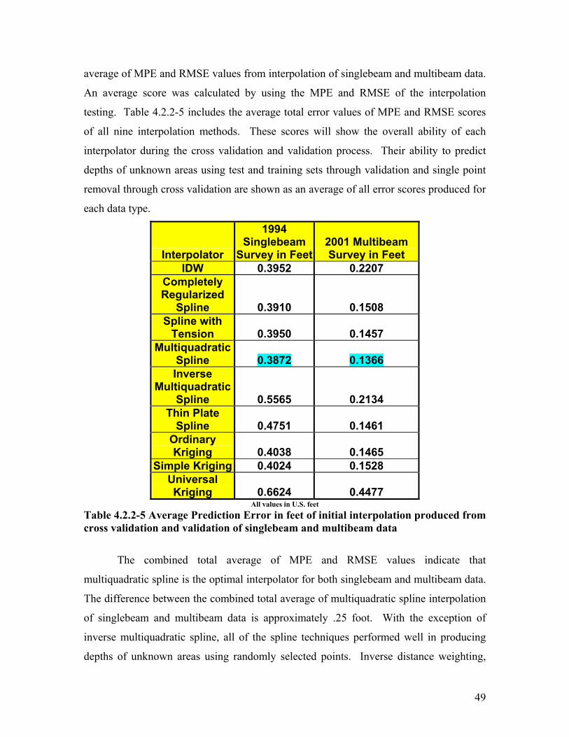
49
average of MPE and RMSE values from interpolation of singlebeam and multibeam data.
An average score was calculated by using the MPE and RMSE of the interpolation
testing. Table 4.2.2-5 includes the average total error values of MPE and RMSE scores
of all nine interpolation methods. These scores will show the overall ability of each
interpolator during the cross validation and validation process. Their ability to predict
depths of unknown areas using test and training sets through validation and single point
removal through cross validation are shown as an average of all error scores produced for
each data type.
Interpolator
1994 Singlebeam
Survey in Feet2001 Multibeam Survey in Feet
IDW 0.3952 0.2207 Completely Regularized
Spline 0.3910 0.1508 Spline with
Tension 0.3950 0.1457 Multiquadratic
Spline 0.3872 0.1366 Inverse
Multiquadratic Spline 0.5565 0.2134
Thin Plate Spline 0.4751 0.1461
Ordinary Kriging 0.4038 0.1465
Simple Kriging 0.4024 0.1528 Universal Kriging 0.6624 0.4477
All values in U.S. feet Table 4.2.2-5 Average Prediction Error in feet of initial interpolation produced from cross validation and validation of singlebeam and multibeam data
The combined total average of MPE and RMSE values indicate that
multiquadratic spline is the optimal interpolator for both singlebeam and multibeam data.
The difference between the combined total average of multiquadratic spline interpolation
of singlebeam and multibeam data is approximately .25 foot. With the exception of
inverse multiquadratic spline, all of the spline techniques performed well in producing
depths of unknown areas using randomly selected points. Inverse distance weighting,

50
ordinary kriging and simple kriging produced similar prediction error values for
singlebeam and multibeam data. Universal kriging and inverse multiquadratic spline
produced the highest and second highest average error for both singlebeam and
multibeam survey data respectively. Table 4.2.2-6 shows the ranking of each interpolator
by survey type while chart 4.2.2-7 shows a comparison of interpolation techniques by
data type.
Interpolator 1994
Singlebeam Survey in Feet
Rank of 1994
Singlebeam Survey
2001 Multibeam Survey in Feet
Rank of 2001 Multibeam
Survey
IDW 0.3952 4 0.2207 8 Completely Regularized
Spline 0.3910 2 0.1508 5
Spline with Tension 0.3950 3 0.1457 2
Multiquadratic Spline 0.3872 1 0.1366 1
Inverse Multiquadratic
Spline 0.5565 8 0.2134 7
Thin Plate Spline 0.4751 7 0.1461 3
Ordinary Kriging 0.4038 6 0.1465 4
Simple Kriging 0.4024 5 0.1528 6 Universal Kriging 0.6624 9 0.4477 9
All values in U.S. feet Table 4.2.2-6 Ranking of interpolation methods using average error for singlebeam and multibeam data

51
Average combined error of validation and cross validation in feet
0
0.1
0.2
0.3
0.4
0.5
0.6
0.7
IDW
Comple
tely R
egula
rized
Spli
ne
Spline
with
Tensio
n
Multiqu
adrat
ic Spli
ne
Invers
e Mult
iquad
ratic
Spline
Thin P
late S
pline
Ordina
ry Krig
ing
Simple
Krig
ing
Univers
al Krig
ing
Interpolator
Erro
r in
Feet
1994 Singlebeam Survey in Feet2001 Multibeam Survey in Feet
Chart 4.2.2-7 A graphical representation of each interpolation method using singlebeam and multibeam data 4.3 Sensitivity Analysis
This section is a discussion of the calculated results from the sensitivity analysis of
singlebeam and multibeam data. The top four performers from the initial testing of
singlebeam and multibeam survey data were chosen and used in this analysis. The
interpolators used in the singlebeam sensitivity analysis are multiquadratic spline,
completely regularized spline, spline with tension, and inverse distance weighting. The
interpolation techniques used in the multibeam sensitivity analysis are multiquadratic
spline, spline with tension, thin plate spline, and ordinary kriging. Each interpolation
method was conducted on ten randomly produced test and training datasets for both 1994
singlebeam survey and 2001 multibeam survey. Each training dataset included 20% of
the total observations while the test dataset included the remaining 80% of the
observations. Cross validation was performed only using 20% (test dataset) of the
observations, while validation used both test and training datasets to derive results. A

52
total of 80 interpolated surfaces were produced in this portion of the analysis.
4.3.1 Singlebeam Sensitivity Analysis
From the four top performing interpolators (multiquadratic spline, completely
regularized spline, spline with tension, and inverse distance weighting), mean predicted
error, RMSE, and mean total error were calculated and recorded to further support the
analysis. Summary and analytical statistics such as mean, sum of error, standard
deviation, 95% confidence intervals (2 standard deviations) were also calculated to
support the decision making process. Ten test and training singlebeam survey datasets
were used in this analysis. Each test and training dataset was created using Microsoft
Excel’s random number generator. Therefore, no test or training dataset contained the
same arrangement of observations.
Tables 4.3.1-1 and 4.3.1-2 give a data description of validation RMSE and MPE
for the sensitivity analysis of singlebeam data. As seen below in table 4.3.1-1, spline
with tension proves to produce the lowest average validation RMSE with a value of
0.7391 feet. Completely regularized spline follows as the second best with
multiquadratic spline and IDW placing third and fourth, respectively. Observing the
confidence intervals for each survey, there is 95% confidence that spline with tension will
vary +/- 0.0166 feet around the mean. Completely regularized spline, the second best
performing interpolator, will vary with 95% confidence +/- 0.0196 feet around the mean.

53
Sample Inverse
Distance Weighting
Completely Regularized
Spline Spline with
Tension Multiquadratic
Spline
1 0.7629 0.7315 0.7355 0.7657 2 0.7528 0.8342 0.7292 0.7463 3 0.7517 0.7233 0.7987 0.7440 4 0.7665 0.7426 0.7227 0.7608 5 0.7707 0.7482 0.7549 0.7593 6 0.7553 0.7565 0.7166 0.7539 7 0.7577 0.7341 0.7403 0.7403 8 0.7604 0.7350 0.7116 0.7488 9 0.7605 0.7504 0.7637 0.7543
10 0.7574 0.7321 0.7180 0.7468
Mean RMSE 0.7595 0.7487 0.7391 0.7520
Standard Deviation 0.0059 0.0316 0.0268 0.0081
95% Confidence
Interval 0.0036 0.0196 0.0166 0.0050
All values in U.S. feet Table 4.3.1-1 Summary and analytical statistics for RMSE of the singlebeam validation sensitivity analysis
Multiquadratic spline proved to produce the lowest validation MPE of 0.0109
with 95% confidence that the MPE will vary +/- 0.0055 feet. Spline with tension, IDW,
and completely regularized spline placed second, third and forth, respectively. All of the
summary and analytical statistics can be seen in table 4.3.1-2.
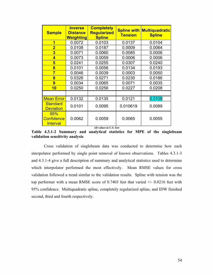
54
Sample Inverse
Distance Weighting
Completely Regularized
Spline Spline with
Tension Multiquadratic
Spline
1 0.0072 0.0103 0.0137 0.0104 2 0.0108 0.0187 0.0009 0.0064 3 0.0071 0.0060 0.0085 0.0006 4 0.0073 0.0059 0.0006 0.0006 5 0.0241 0.0255 0.0307 0.0240 6 0.0101 0.0056 0.0134 0.0193 7 0.0046 0.0039 0.0003 0.0050 8 0.0326 0.0271 0.0230 0.0186 9 0.0034 0.0065 0.0071 0.0035
10 0.0250 0.0256 0.0227 0.0208
Mean Error 0.0132 0.0135 0.0121 0.0109 Standard Deviation 0.0101 0.0095 0.010619 0.0089
95% Confidence
Interval 0.0062 0.0059 0.0065 0.0055
All values in U.S. feet Table 4.3.1-2 Summary and analytical statistics for MPE of the singlebeam validation sensitivity analysis
Cross validation of singlebeam data was conducted to determine how each
interpolator performed by single point removal of known observations. Tables 4.3.1-3
and 4.3.1-4 give a full description of summary and analytical statistics used to determine
which interpolator performed the most effectively. Mean RMSE values for cross
validation followed a trend similar to the validation results. Spline with tension was the
top performer with a mean RMSE score of 0.7403 feet that varied +/- 0.0216 feet with
95% confidence. Multiquadratic spline, completely regularized spline, and IDW finished
second, third and fourth respectively.

55
Sample Inverse
Distance Weighting
Completely Regularized
Spline Spline with
Tension Multiquadratic
Spline
1 0.7742 0.739 0.7427 0.779 2 0.7863 0.9014 0.7595 0.7756 3 0.7725 0.744 0.8265 0.7634 4 0.7506 0.7352 0.7083 0.7438 5 0.7433 0.7214 0.7267 0.7397 6 0.7599 0.7556 0.7136 0.7476 7 0.7602 0.7275 0.7334 0.7446 8 0.7803 0.7619 0.7401 0.7796 9 0.7521 0.7423 0.7456 0.739
10 0.7452 0.7287 0.7066 0.726
Mean RMSE 0.7624 0.7557 0.7403 0.7538
Standard Deviation 0.0150 0.0526 0.0348 0.0190
95% Confidence
Interval 0.0093 0.0326 0.0216 0.0118
All values in U.S. feet Table 4.3.1-3 Summary and analytical statistics for RMSE of the singlebeam cross validation sensitivity analysis Mean prediction error for cross validation can be seen in table 4.3.1-4.
Multiquadratic spline produced the lowest MPE with a score 0.0109 feet. With 95%
confidence, multiquadratic spline will also produce scores that will vary +/- 0.0055 feet
around the mean. This score is the lowest of all the interpolators tested in this portion of
the sensitivity analysis. Spline with Tension and IDW ranked second and third
respectively, while completely regularized spline ranked fourth.

56
Sample Inverse
Distance Weighting
Completely Regularized
Spline Spline with
Tension Multiquadratic
Spline
1 0.0072 0.0103 0.0137 0.0104 2 0.0108 0.0187 0.0009 0.0064 3 0.0071 0.0060 0.0085 0.0006 4 0.0073 0.0059 0.0006 0.0006 5 0.0241 0.0255 0.0307 0.0240 6 0.0102 0.0056 0.0134 0.0193 7 0.0046 0.0039 0.0003 0.0050 8 0.0326 0.0271 0.0230 0.0186 9 0.0034 0.0065 0.0071 0.0035
10 0.0250 0.0256 0.0227 0.0208
Mean Error 0.0132 0.01356 0.0121 0.0109 Standard Deviation 0.0101 0.0095 0.0106 0.0089
95% Confidence
Interval 0.0062 0.0059 0.0065 0.0055
All values in U.S. feet
Table 4.3.1-4 Summary and analytical statistics for MPE of the singlebeam cross validation sensitivity analysis Average error was calculated for both RMSE and MPE of the validation and cross
validation for singlebeam data. These scores are average total error in U.S. feet. Table
4.3.1-5 shows each interpolator’s performance rating along with summary and analytical
statistics that aided in the decision process of choosing the optimal interpolator. Spline
with tension proved to be the top performing interpolator using singlebeam data. While
multiquadratic spline produced the lowest MPE scores, it did not produce the lowest
RMSE scores. Multiquadratic spline had a 95% confidence interval that varied +/-
0.0040 feet around the mean average error while spline with tension produced a 95%
confidence interval that varied +/- 0.0090 feet around the mean. Even though
multiquadratic spline has the least variability of error in the ten samples tested, it is still
optimal to choose spline with tension because it produced the lowest average error using
singlebeam data and computation time was notably faster.

57
Sample
Inverse Distance
Weighting
Completely Regularized
Spline Spline with
Tension Multiquadratic
Spline 1 0.3878 0.3727 0.3764 0.3913 2 0.39015 0.4432 0.3726 0.3836 3 0.3846 0.3698 0.4105 0.3771 4 0.3829 0.3724 0.3580 0.3764 5 0.3905 0.3801 0.3857 0.3867 6 0.3838 0.3808 0.3642 0.3850 7 0.3817 0.3673 0.3685 0.3737 8 0.4014 0.3877 0.3744 0.3914 9 0.3798 0.3764 0.3808 0.3750
10 0.3881 0.3780 0.3675 0.3786 RANK 4 3 1 2
Mean Error 0.3871 0.3828 0.3759 0.3819 Standard Deviation 0.0061 0.0220 0.0145 0.0066
95% Confidence
Interval 0.0038 0.0136 0.0090 0.0040
All values in US feet
Table 4.3.1-5 Average Prediction error of validation and cross validation for interpolation sensitivity analysis using singlebeam data 4.3.2 Multibeam Sensitivity Analysis From the four chosen interpolators (multiquadratic spline, ordinary kriging, spline
with tension, and thin plate spline) mean predicted error, RMSE, and Average error were
observed and recorded to further support the analysis. Summary and analytical statistics
such as mean, sum of error, standard deviation, 95% confidence intervals (2 standard
deviations) were also calculated to support the decision making process. Ten test and
training multibeam survey datasets were used in this analysis. Each test and training
dataset was created using Microsoft Excel’s random number generator. Therefore, no
test or training dataset contained the same arrangement of observations.
Validation testing of the 2001 dataset was conducted using ten differently
arranged samples. RMSE and MPE values can be seen in tables 4.3.2-1 and 4.3.2-2. Of
the four interpolators tested, thin plate spline produced the lowest validation mean RMSE
of 0.2874 feet. Spline with tension produced the second lowest mean RMSE value

58
followed by ordinary kriging and multiquadratic spline. Ironically, multiquadratic spline
produced the highest validation mean RMSE in initial interpolation testing. This
difference in scores indicates that spatial arrangement of observations plays an important
role in the performance level of multiquadratic spline.
Sample Ordinary Kriging
Thin Plate Spline
Spline with Tension
Multiquadratic Spline
1 0.2996 0.2831 0.2811 0.2902 2 0.2867 0.2878 0.2876 0.3381 3 0.2879 0.2898 0.2875 0.3331 4 0.2871 0.2978 0.2875 0.3239 5 0.3011 0.2941 0.3002 0.3249 6 0.3050 0.2844 0.2839 0.3058 7 0.2674 0.2825 0.2823 0.2856 8 0.2800 0.2815 0.2808 0.3255 9 0.2827 0.2840 0.3031 0.3734 10 0.2968 0.2895 0.2889 0.3575
Mean RMSE 0.2894 0.2874 0.2882 0.3258 Standard Deviation 0.0114 0.0053 0.0076 0.0274
95% Confidence
Interval 0.0070 0.0033 0.0047 0.0169
All values in U.S. feet Table 4.3.2-1 Summary and analytical statistics for RMSE of the multibeam validation sensitivity analysis
Validation mean prediction error values for multibeam data can be seen in table
4.3.2-2. Ordinary kriging produced the lowest mean prediction error with a value of
0.0019 feet. Spline with tension produced the second lowest MPE with a value of
0.0032. Thin plate spline and multiquadratic spline produced the third and fourth lowest
scores, respectively. Ordinary kriging also produced the smallest 95% confidence
interval which indicates there is small variability in MPE produced when tested on
randomly arranged samples.

59
Sample Ordinary Kriging
Thin Plate Spline
Spline with Tension
Multiquadratic Spline
1 0.0001 0.0022 0.0019 0.0013 2 0.0076 0.0068 0.0068 0.0062 3 0.0004 0.0088 0.0068 0.0062 4 0.0002 0.0068 0.0068 0.0061 5 0.0012 0.0022 0.0011 0.0020 6 0.0008 0.0014 0.0014 0.0009 7 0.0007 0.0001 0.0002 0.0006 8 0.0028 0.0036 0.0037 0.0062 9 0.0017 0.0021 0.0024 0.0039 10 0.0040 0.0006 0.0006 0.0037
Mean Error 0.0019 0.0035 0.0032 0.0037 Standard Deviation 0.0023 0.0029 0.0027 0.0023
95% Confidence
Interval 0.0014 0.0018 0.0016 0.0014
All values in U.S. feet Table 4.3.2-2 Summary and analytical statistics for MPE of the multibeam validation sensitivity analysis
Cross validation statistics produced from the sensitivity analysis of multibeam
data can be seen in tables 4.3.2-3 and 4.3.2-4. Spline with tension produced the lowest
cross validation RMSE of 0.2850 feet with 95% confidence that the RMSE will vary +/-
0.0055 feet. Multiquadratic spline produced the highest mean RMSE of 0.3376 feet with
95% confidence that it will vary +/- 0.0212 feet around the mean.
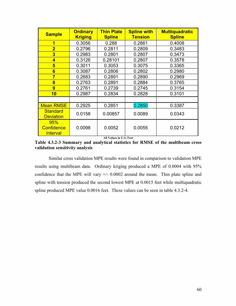
60
Sample Ordinary Kriging
Thin Plate Spline
Spline with Tension
Multiquadratic Spline
1 0.3056 0.288 0.2861 0.4008 2 0.2796 0.2811 0.2809 0.3483 3 0.2983 0.2801 0.2807 0.3473 4 0.3126 0.28101 0.2807 0.3578 5 0.3011 0.3053 0.3075 0.3365 6 0.3087 0.2806 0.2802 0.2980 7 0.2683 0.2891 0.2890 0.2969 8 0.2763 0.2891 0.2884 0.3765 9 0.2761 0.2739 0.2745 0.3154 10 0.2987 0.2834 0.2828 0.3101
Mean RMSE 0.2925 0.2851 0.2850 0.3387 Standard Deviation 0.0158 0.00857 0.0089 0.0343
95% Confidence
Interval 0.0098 0.0052 0.0055 0.0212
All Values in U.S. Feet Table 4.3.2-3 Summary and analytical statistics for RMSE of the multibeam cross validation sensitivity analysis Similar cross validation MPE results were found in comparison to validation MPE
results using multibeam data. Ordinary kriging produced a MPE of 0.0004 with 95%
confidence that the MPE will vary +/- 0.0002 around the mean. Thin plate spline and
spline with tension produced the second lowest MPE at 0.0015 feet while multiquadratic
spline produced MPE value 0.0016 feet. These values can be seen in table 4.3.2-4.
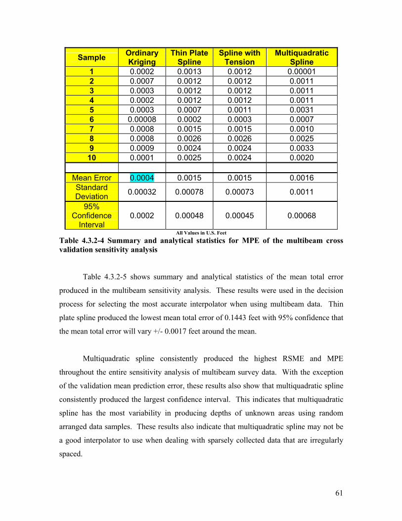
61
Sample Ordinary Kriging
Thin Plate Spline
Spline with Tension
Multiquadratic Spline
1 0.0002 0.0013 0.0012 0.00001 2 0.0007 0.0012 0.0012 0.0011 3 0.0003 0.0012 0.0012 0.0011 4 0.0002 0.0012 0.0012 0.0011 5 0.0003 0.0007 0.0011 0.0031 6 0.00008 0.0002 0.0003 0.0007 7 0.0008 0.0015 0.0015 0.0010 8 0.0008 0.0026 0.0026 0.0025 9 0.0009 0.0024 0.0024 0.0033 10 0.0001 0.0025 0.0024 0.0020
Mean Error 0.0004 0.0015 0.0015 0.0016 Standard Deviation 0.00032 0.00078 0.00073 0.0011
95% Confidence
Interval 0.0002 0.00048 0.00045 0.00068
All Values in U.S. Feet Table 4.3.2-4 Summary and analytical statistics for MPE of the multibeam cross validation sensitivity analysis
Table 4.3.2-5 shows summary and analytical statistics of the mean total error
produced in the multibeam sensitivity analysis. These results were used in the decision
process for selecting the most accurate interpolator when using multibeam data. Thin
plate spline produced the lowest mean total error of 0.1443 feet with 95% confidence that
the mean total error will vary +/- 0.0017 feet around the mean.
Multiquadratic spline consistently produced the highest RSME and MPE
throughout the entire sensitivity analysis of multibeam survey data. With the exception
of the validation mean prediction error, these results also show that multiquadratic spline
consistently produced the largest confidence interval. This indicates that multiquadratic
spline has the most variability in producing depths of unknown areas using random
arranged data samples. These results also indicate that multiquadratic spline may not be
a good interpolator to use when dealing with sparsely collected data that are irregularly
spaced.

62
Sample Ordinary Kriging
Thin Plate Spline
Spline with Tension
Multiquadratic Spline
1 0.15137 0.1436 0.1425 0.1730 2 0.1436 0.1442 0.1441 0.1734 3 0.1467 0.1449 0.1440 0.1719 4 0.1500 0.1467 0.1440 0.1722 5 0.1509 0.1505 0.1524 0.1666 6 0.1536 0.1416 0.1414 0.1513 7 0.1343 0.1433 0.1432 0.1460 8 0.1399 0.1442 0.1438 0.1776 9 0.1403 0.1406 0.1456 0.1740 10 0.1499 0.1440 0.1436 0.1683
RANK 3 1 2 4 Mean Error 0.1460 0.1443 0.1445 0.1674 Standard Deviation 0.0062 0.0027 0.0029 0.0104
95% Confidence
Interval 0.0038 0.0017 0.0018 0.0064
All values in U.S. Feet
Table 4.3.2-5 Mean total error of validation and cross validation for interpolation sensitivity analysis using multibeam data
4.4 Sensitivity Analysis Results
The final results of this portion of the sensitivity analysis are as follows: spline
with tension produced the lowest mean total error using singlebeam data while thin plate
spline produced the lowest mean total error using multibeam data. Both of these
interpolators produced the lowest mean total error when using randomly arranged
observations from singlebeam and multibeam hydrographic surveys. Multiquadratic
spline produced the highest mean total error when predicting unknown depths of
multibeam survey data. Inverse distance weighting produced the highest mean total error
when predicting unknown depths of singlebeam survey data. Charts 4.4-1 and 4.4-2
provide a visual display of each interpolator’s performance using singlebeam and
multibeam data.

63
Average Prediction Error of Validation and Cross Validation for Interpolation of Singlebeam Data
0
0.1
0.2
0.3
0.4
0.5
1 2 3 4 5 6 7 8 9 10
Test/ Training Dataset Number
Ave
rage
Err
or in
Fee
tInverse DistanceWeightingCompletely RegularizedSplineSpline with Tension
Multiquadratic Spline
Chart 4.4-1 Average error of validation and cross validation for interpolation of
singlebeam data
Average Prediction Error of Validation and Cross validation of Multibeam data
0
0.05
0.1
0.15
0.2
1 2 3 4 5 6 7 8 9 10
Test/ Training Dataset Number
Ave
rage
Err
or in
Fee
t
Ordinary KrigingThin Plate SplineSpline with TensionMultiquadratic Spline
Chart 4.4-2 Average error of validation and cross validation for interpolation of
multibeam data

64
4.4.1 Paired t Tests
Paired T – Tests were conducted to determine if a significant difference in the
mean value existed among the interpolators used in the singlebeam data and multibeam
data sensitivity analysis. Each of the four interpolators used in both dataset analyses
were paired and tested to determine if evidence existed that there is a significant
difference in the total mean error produced by each interpolator. Table 4.5.1-2 and 4.5.1-
3 show the t – value, degrees of freedom, and p – value of each interpolation pairing for
singlebeam and multibeam data. The statistical software used for this portion of the
analysis was NCSS. The null hypothesis for the paired t- test states that the mean
difference of all matched pairs equals zero (McGrew and Monroe, 2000). The alternative
hypothesis for this test states that the mean difference is greater than, less than, or not
equal to zero (McGrew and Monroe, 2000). The decision level to determine whether to
reject or accept the null hypothesis is α = 0.05. Figure 4.5.1-1 shows the hypotheses used
in this testing.
Hypothesis:
Ho: µ1 = µ2
Ha: µ1 ≠ µ2 (two-tailed)
Ha: µ1 > µ2 (one tailed)
Ha: µ1 < µ2 (one tailed)
Figure 4.4.1-1 Hypotheses of matched – pairs t Test
4.4.2 Discussion of matched-pair t- Test Shown in table 4.4.2-1 listed below, with 95% confidence level, IDW was found
to be significantly different in the mean prediction error produced in comparison to
multiquadratic spline and spline with tension. The matched pair t – Test of interpolators
using singlebeam data reported that t – Test numbers 3 – 6 showed no significant
difference in the mean absolute combined prediction error. The matched pair t –Test of
multibeam interpolators (table 4.4.2-2) showed with 95 % confidence level that t –Test
numbers 1-3 were significantly different in the mean absolute combined prediction error

65
produced. The t – Tests also concluded that t - Test numbers 4 – 6 found no significant
difference in the mean absolute combined prediction errors produced.
t-Test Number
Interpolation Pairing t df p-value Decision
(5%)
1 IDW & Spline w/ Tension 2.26 10 0.050 Reject Ho
2 IDW &
Multiquadratic Spline
3.71 10 0.005 Reject Ho
3 IDW & Completely Regularized Spline 0.65 10 0.530 Accept Ho
4 Completely
Regularized Spline & Spline w/
Tension 0.79 10 0.450 Accept Ho
5 Completely
Regularized Spline & Multiquadratic
Spline 0.14 10 0.891 Accept Ho
6 Spline w/ Tension & Multiquadratic
Spline -1.18 10 0.268 Accept Ho
Table 4.4.2-1 Matched Pairs t Test of the mean total error from the singlebeam survey sensitivity analysis
t-Test Number
Interpolation Pairing t df p-value Decision
(5%)
1 Multiquadratic
Spline & Spline w/ Tension
7.03 10 0.000 Reject Ho
2 Multiquadratic
Spline & Thin Plate Spline
7.06 10 0.000 Reject Ho
3 Multiquadratic
Spline & Ordinary Kriging
5.87 10 0.000 Reject Ho
4 Spline w/ Tension & Thin Plate Spline 0.22 10 0.833 Accept Ho
5 Spline w/ Tension & Ordinary Kriging - 0.73 10 0.484 Accept Ho
6 Thin Plate Spline & Ordinary Kriging - 0.90 10 0.393 Accept Ho
Table 4.4.2-2 Matched Pairs t Test of the mean total error from the multibeam survey sensitivity analysis

66
Interpolation Pairing Singlebeam Sensitivity Analysis
Reject Ho Accept Ho
IDW I Spline w/ Tension I Completely Regularized Spline I I Multiquadratic Spline I Table 4.4.2-3 Dendrogram of t – test results from singlebeam sensitivity analysis
Figures 4.4.2-3 and 4.4.2-4 show which interpolators have a significant difference
in mean total error. Interpolators that have a mark in the alternative hypothesis column
(reject Ho) have a significant difference in the mean total error. Those interpolators that
have a mark in the null hypothesis column (Accept Ho) display no significant difference
in the mean total error.
Interpolation Pairing Multibeam Sensitivity Analysis
Reject Ho
Accept Ho
Multiquadratic Spline I Thin Plate Spline I I Ordinary Kriging I I Spline w/ Tension I I Table 4.4.2-4 Dendrogram of t-test results from multibeam sensitivity analysis

67
4.5 Highest and Lowest Error Producing Interpolators
Sample Number
Average Error of Spline with
Tension Average Error of Universal Kriging
1 0.3729 0.5652 2 0.3729 0.6636 3 0.4093 0.6527 4 0.3581 0.6582 5 0.3784 0.6582 6 0.3613 0.6476 7 0.3689 0.6391 8 0.3688 0.6481 9 0.3796 0.6150 10 0.3618 0.6545 11 0.3758 0.6580 12 0.3901 0.6531 13 0.3973 0.6259 14 0.3802 0.6850 15 0.3660 0.6513 16 0.3833 0.6617 17 0.3764 0.6499 18 0.3671 0.6452 19 0.3787 0.6435 20 0.3604 0.6526 21 0.3644 0.6466 22 0.4139 0.6390 23 0.3612 0.6531 24 0.3788 0.6514 25 0.3648 0.6462 26 0.4110 0.6582 27 0.4052 0.6491 28 0.3771 0.6557 29 0.3709 0.6978 30 0.3708 0.6978
All values in U.S. Feet
Table 4.5-1 Mean total error produced from validation and cross validation
This section addresses the
likelihood that overlap in the
range of error may exist between
the lowest error producing
interpolator and highest error
producing interpolator. Spline
with tension, the lowest error
producing interpolator for
singlebeam data and universal
kriging, the highest error
producing interpolator for
singlebeam data were used for
this portion of the analysis. A
multibeam data investigation was
not conducted due to the lengthy
calculation time of universal
kriging.
Validation and cross
validation was performed using
30 randomly generated test and
training datasets. RMSE and
MPE values were produced from
both validation and cross
validation. Table 4.5-1 list the
mean total error values produced
by spline with tension
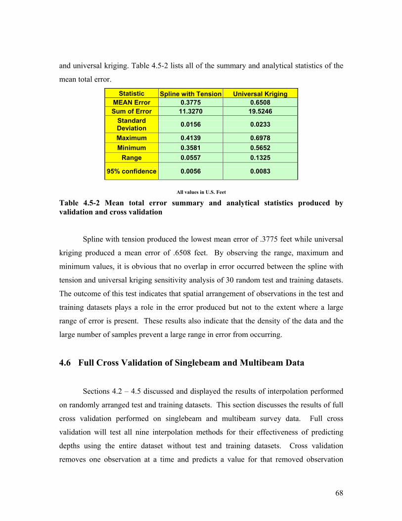
68
and universal kriging. Table 4.5-2 lists all of the summary and analytical statistics of the
mean total error.
Statistic Spline with Tension Universal Kriging MEAN Error 0.3775 0.6508 Sum of Error 11.3270 19.5246
Standard Deviation 0.0156 0.0233
Maximum 0.4139 0.6978 Minimum 0.3581 0.5652
Range 0.0557 0.1325
95% confidence 0.0056 0.0083
All values in U.S. Feet
Table 4.5-2 Mean total error summary and analytical statistics produced by validation and cross validation Spline with tension produced the lowest mean error of .3775 feet while universal
kriging produced a mean error of .6508 feet. By observing the range, maximum and
minimum values, it is obvious that no overlap in error occurred between the spline with
tension and universal kriging sensitivity analysis of 30 random test and training datasets.
The outcome of this test indicates that spatial arrangement of observations in the test and
training datasets plays a role in the error produced but not to the extent where a large
range of error is present. These results also indicate that the density of the data and the
large number of samples prevent a large range in error from occurring.
4.6 Full Cross Validation of Singlebeam and Multibeam Data
Sections 4.2 – 4.5 discussed and displayed the results of interpolation performed
on randomly arranged test and training datasets. This section discusses the results of full
cross validation performed on singlebeam and multibeam survey data. Full cross
validation will test all nine interpolation methods for their effectiveness of predicting
depths using the entire dataset without test and training datasets. Cross validation
removes one observation at a time and predicts a value for that removed observation

69
based on the rest of the known observations. The known value is then compared to the
predicted value and a grid is produced. RMSE and MPE values are calculated and
compared to determine the effectiveness of each interpolator. Tables 4.6-1 and 4.6-3 list
the MPE and RMSE produced by interpolation of singlebeam and multibeam data.
Figures 4.6-2 and 4.6-4 display the filled contour maps produced by each interpolator.
The red line on each contour map is an outline of the Atlantic Ocean Channel.
Interpolator MPE RMSE Mean Total Error Rank
IDW 0.0009 0.58 0.5809 6 Completely
Regularized Spline 0.0005 0.572 0.5725 5
Spline with Tension 0.0002 0.5187 0.5189 2
Thin Plate Spline 0.00006 0.5165 0.5165 1
Multiquadratic Spline 0.0001 0.5211 0.5212 3
Inverse Multiquadratic Spline 0.0010 0.5211 0.5221 4
Ordinary Kriging 0.0029 0.6603 0.6632 7 Simple Kriging 0.0031 0.6634 0.6665 8
Universal Kriging 0.0160 0.9350 0.9510 9 All Values in U.S. Feet
Table 4.6-1 MPE, RMSE, and Mean total error of full cross validation using 1994 singlebeam survey data For the full cross validation analysis of singlebeam data, thin plate spline
produced the lowest average total error of 0.5165 feet. Spline with tension produced an
average total error of 0.5189 feet and multiquadratic spline produced an average total
error of 0.5212 feet. The rest of the values can be seen above in table 4.6-1. Figure 4.6-2
displays all contour surfaces produced by each interpolation method using singlebeam
hydrographic survey data. The red line visible on each contoured surface is the channel
plan form of the Atlantic Ocean Channel. Only the interpolated area was used in
producing error statistics and for further analysis.

70
Inverse Distance Weighting Completely Regularized Spline
Spline with Tension Thin plate Spline
Multiquadratic Spline Inverse Multiquadratic Spline
Figure 4.6-1 Filled contour maps of estimated depth using singlebeam survey data (continued on next page)

71
Ordinary Kriging Simple Kriging
Universal Kriging
Figure 4.6-1 (continued) Filled contour maps of estimated depth using singlebeam survey data
Because the range of mean total error of the full cross validation for all
interpolators is approximately 0.44 feet, noticeable difference of each contour surface is
difficult to observe. The red line on each map is an outline of the Atlantic Ocean
Channel. Each interpolator produced surfaces to the maximum and minimum X, Y
coordinates of the Atlantic Ocean Channel. Only the contour area within the channel
boundary will be used to calculate volume of sediment for each survey used in this
analysis.
Legend In Feet

72
Interpolator MPE RMSE Average Total Error Rank
IDW 0.0001 0.2271 0.2272 6 Completely Regularized
Spline 0.0005 0.2115 0.2120 4
Spline with Tension 0.0027 0.774 0.7767 9
Thin Plate Spline 0.0001 0.1686 0.1687 2 Multiquadratic
Spline 0.0005 0.1791 0.1796 3
Inverse Multiquadratic
Spline 0.0005 0.3635 0.3640 7
Ordinary Kriging 0.0002 0.2126 0.2128 5 Simple Kriging 0.0005 0.1495 0.1500 1
Universal Kriging 0.0044 0.4784 0.4828 8 All Values in U.S. Feet
Table 4.6-2 MPE, RMSE, and Average error of full cross validation using 2001 multibeam survey data For full cross validation of multibeam survey data, simple kriging produced the
lowest mean total error of 0.1500 feet. Thin plate spline performed well in producing a
low mean total error of 0.1687 feet. Multiquadratic spline was the third most effective
while completely regularized spline was the fourth most effective in predicting depths
through cross validation. The display of mean total error produced by each interpolator
can be seen above in table 4.6-3. Figure 4.6-4 displays all contour surfaces produced by
each interpolation method using multibeam hydrographic survey data. The red line
visible on each contoured surface is the channel plan form of the Atlantic Ocean Channel.
Only the interpolated area was used in producing error statistics and for further analysis.

73
Inverse Distance Weighting Completely Regularized Spline
Spline with Tension Thin Plate Spline
Multiquadratic Spline Inverse Multiquadratic Spline
Figure 4.6-2 Filled contour maps of estimated depth using multibeam survey data (continued on next page)
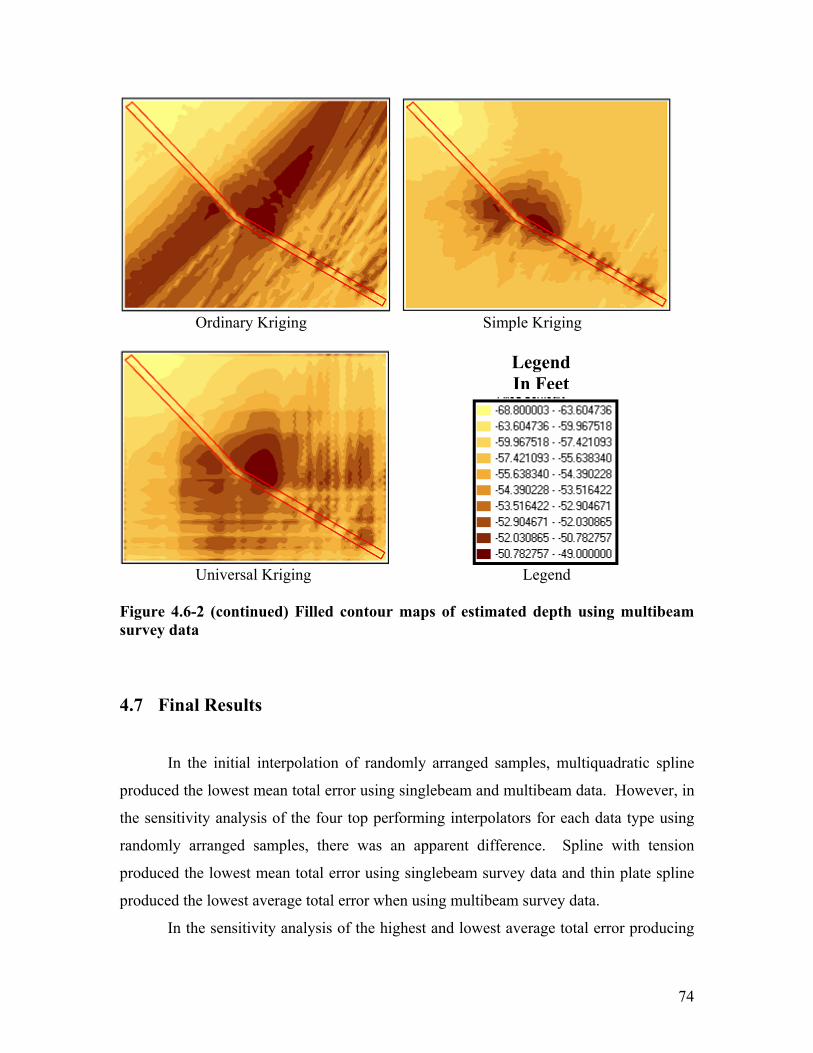
74
Ordinary Kriging Simple Kriging
Universal Kriging Legend Figure 4.6-2 (continued) Filled contour maps of estimated depth using multibeam survey data
4.7 Final Results
In the initial interpolation of randomly arranged samples, multiquadratic spline
produced the lowest mean total error using singlebeam and multibeam data. However, in
the sensitivity analysis of the four top performing interpolators for each data type using
randomly arranged samples, there was an apparent difference. Spline with tension
produced the lowest mean total error using singlebeam survey data and thin plate spline
produced the lowest average total error when using multibeam survey data.
In the sensitivity analysis of the highest and lowest average total error producing
Legend In Feet

75
interpolators, there was no evident overlap of error produced by the thirty randomly
arranged samples. Spline with tension produced mean total error scores that were
approximately .3 feet smaller in comparison to universal kriging.
Full cross validation produced results that were somewhat dissimilar to the
sensitivity analysis results of randomly arranged datasets. Thin plate spline produced the
lowest mean total error for full cross validation of singlebeam survey data. Thin plate
spline was the best performing interpolator for the previous sensitivity analysis using
randomly arranged and withheld multibeam data. Simple kriging produced the lowest
average total error for full cross validation of multibeam data survey data. Simple
kriging was very effective in producing low mean prediction error values in the
sensitivity analysis of randomly arranged and withheld singlebeam and multibeam data.
In this portion of the analysis, it proved to be the optimal interpolator.
In choosing an interpolator for creating grids and for use in volume analysis,
spline with tension was chosen when using singlebeam data and thin plate spline was
chosen for use with multibeam data. These interpolators were chosen for their ability to
produce the lowest average total error when exposed to randomly located data
observations. Splines are also computationally efficient and less subjective to criticism in
comparison to most kriging methods. Inverse distance weighting is computationally
efficient but produces high mean total error when randomly arranged data and full
datasets in comparison to most splines and most kriging techniques.

76
5 Volume Analysis 5.1 Overview
This chapter includes a complete discussion of the calculated sediment increase of
the Atlantic Ocean Channel. Discussed in this chapter are the spatial interpolators used
to produce grids from singlebeam and multibeam hydrographic surveys. Also, the
comparison of calculated volumes using TINs and varying grid resolutions is also
reported. The last topic of this chapter is a description and summary of the shoaling rate
present in the Atlantic Ocean Channel.
5.2 Volume Calculations
Using singlebeam hydrographic and multibeam hydrographic survey data, 15
meter, 30 meter, 60 meter, and 90 meter grids were produced to determine at what rate
the Atlantic Ocean Channel was shoaling. These varying grid resolutions were also
created to see how the decrease in grid resolution affected the volume calculations.
These grids were also compared to the volume calculations of TIN models, the USACE’s
model of choice for determining channel conditions using sparse cross sectional data.
Grids were created at 15m, 30m, 60m, and 90m to determine if varying resolution
affected volume calculations and to ultimately answer whether or not the Atlantic Ocean
Channel is indeed shoaling. Also to be answered is at what rate is the Atlantic Ocean
Channel shoaling. Shoaling is identified as the accumulation and increase of sediment
volume in a navigation channel over time. To properly quantify shoaling rates, sediment
must be measured over a plan depth. A plan depth is a reference depth that remains
constant regardless of when each survey was recorded. Two surveys with different
recording dates of the same channel cannot be compared to determine sediment increase.
This technique can only be used if the surveyor adequately addresses the inherent
measurement error of both surveys and can quantify the increased error of volumes
produced by comparing two different surveys of the same location (USACE, 2002). The

77
chance that a survey point from one year’s survey will be taken in the exact same location
in the following year is highly unlikely.
5.2.1 Grid Development
The spatial interpolators used to create grids from singlebeam and multibeam
survey data are as follows: spline with tension was used to produce grids from the 1994,
1996, 1999 singlebeam hydrographic survey and thin plate spline was used to create grids
from the 2000 and 2001 multibeam hydrographic survey. As discussed in Chapter 4,
spline interpolators were chosen to produce grids because they produced the lowest mean
total error from randomly arranged samples. They also produced low mean total error
scores from entire surveys. Spline interpolators are also computationally efficient
compared to kriging interpolators, which are computationally inefficient. Figures 5.2-1
– 5.2-5 displays the MPE and RMSE produced from cross validation of each singlebeam
and multibeam survey. Each figure also displays the linear regression of predicted versus
known observation. By looking at the regression plots, there are linear slope factors of
98.7 to 100% among each cross validation procedure, which indicates a strong positive
linear correlation.
Figure 5.2-1 Cross validation of the 1994 singlebeam hydrographic survey

78
Figure 5.2-2 Cross validation of the 1996 singlebeam hydrographic survey
Figure 5.2-3 Cross validation of the 1999 singlebeam hydrographic survey
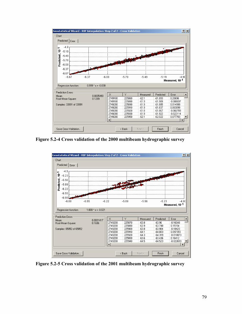
79
Figure 5.2-4 Cross validation of the 2000 multibeam hydrographic survey
Figure 5.2-5 Cross validation of the 2001 multibeam hydrographic survey

80
By observing each regression plot, it is evident that multibeam hydrographic
survey data produces a stronger correlation between known and predicted variables in
cross validation compared to singlebeam hydrographic survey data. This will ultimately
affect the accuracy of the grids produced. Multibeam hydrographic survey data will
produce sediment volumes with greater accuracy due to increased survey point density
within the Atlantic Ocean Channel.
5.2.2 Volume Estimates
After interpolation, grids were created at varying resolutions and volume
estimates were produced at a 53-foot plan depth level. This plan depth was chosen
because it will be implemented by the USACE for future deepening projects of the
Atlantic Ocean Channel. Grids were constructed from each survey year and type at 15m,
30m, 60m, and 90m, resolution. A total of 20 grids were produced in this portion of the
analysis. TIN models were also produced to compare sediment calculation amounts
against grid produced sediment amounts. Table 5.2-1 is a listing of volume of sediment
above 53 feet deep in the Atlantic Ocean Channel. Each volume was calculated using the
ArcGIS 3D Analyst.
Survey Year 15 Meter 30 Meter 60 Meter 90 Meter TIN
1994 54,996 29,439 16,001 5,413 73,0921996 3,240,041 2,893,045 2,263,021 1,845,080 3,431,8591999 4,257,347 3,861,480 3,071,045 2,330,658 4,501,1822000 6,158,897 5,617,398 4,583,492 3,575,683 6,471,3312001 6,132,944 5,595,816 4,559,103 3,568,288 6,575,988
Average Increase
of sediment per year
868,278 795,197 649,015 508,982 928,985
Unit in Cubic Yards
Table 5.2.2-1 Estimated volume of sediment above plan depth for TIN models and
varying Grid resolution

81
Chart 5.2.2-1 & 5.2.2-2 provide a visual display of the difference of volume
calculations between varying grid resolutions and TIN modeling. It is evident that the
Atlantic Ocean Channel is indeed shoaling from 1994 through 2000. In 2001, there is a
subtle decline in the volume of sediment present above 53 feet in the channel.
Chart 5.2.2-1 Volume estimates of varying grid resolution models and TIN models
Chart 5.2.2-2 Volume estimate produced by grid and TIN modeling
Volume Estimates from TINs and Grids
0
1,000,000
2,000,000
3,000,000
4,000,000
5,000,000
6,000,000
7,000,000
1994 1996 1999 2000 2001
Year of Survey
Cub
ic Y
ards
of S
edim
ent
15 Meter30 Meter60 Meter90 MeterTIN
Estimated Volumes produced by varying Grid resolutions and TIN modeling
01,000,0002,000,0003,000,0004,000,0005,000,0006,000,0007,000,000
1994 1996 1999 2000 2001
Survey Year
Volu
me
in C
ubic
Yar
ds
15 Meter30 Meter60 Meter90 MeterTIN

82
Varying grid resolutions had a significant impact on the estimation of sediment
volume above a plan depth of 53 feet. Smoothing each channel surface generalizes the
depths and anomalies that may exist on the channel bottom. Therefore, a smaller grid
cell will provide a more accurate depiction of depth and will be able to estimate sediment
volume more accurately. Increasing cell size reduces the accuracy of the surface by
taking the average depth of data points within the cell’s area of extent. This method does
not allow for localized shoaling to be identified. TIN modeling proved to produce the
highest sediment volumes. TINs produce areas by using each depth reading as a mass
point. Table 5.2-2 listed below shows a percentage of increase in sediment volume from
1994 - 2001. This percentage increase indicates that an increase in cell area does not
allow for accurate volume calculations because it will not be able to calculate sediment
depths that are marginally above the plan depth. A grid cell of less than 15 meters would
possibly prove to estimate sediment volumes more accurately than TINs.
Grid Resolution
15 meter 30 meter 60 meter 90 meter
Percentage Increase from 1994 - 2001
11,100% 19,000% 28,400% 65,900%
Table 5.2.2-2 Estimated percentage increase of sediment volume by varying grid
resolution
5.3 Interpolation and Volume Error
The USACE standards indicate that survey accuracy for deep-water entrance
channels must have a vertical error tolerance no greater than +/- 2.0 feet. With the
exception of universal kriging applied to singlebeam hydrographic survey data, all
interpolation methods produce a mean total error lower than 2.0 feet. This error total
encompasses both validation and cross validation error. Also noted is the fact that the
error produced is determined from validation and cross validation of neighboring points
in a transect. Cross-section points are spaced 20 feet apart but the transects are spaced
100 – 400 feet apart. It should be mentioned that the reported error in this research is

83
lower than the actual error. The actual error could be determined if more surveying, in
coordination with cross-section surveys, were conducted parallel to the channel direction.
With more depth observations, a more accurate surface could be interpolated which could
be used to estimate sediment volume more accurately.
The error that is produced by interpolation ultimately effects sediment volume
calculations. The USACE’s Engineering and Design Hydrographic Surveying (2002)
document states that bias in a survey must be recognized and calculated into the dredge
design and volume payment. If 0.1 feet of error bias exists in an area that is 400ft x
3,000ft, approximately 4,450 cubic yards of sediment could be unaccounted for or
unnecessarily dredged. Bias error can become more significant in offshore tidal areas
where modeling becomes more difficult.
Volume error = 0.1ft * 400ft * 3,000ft / (27 cy/ft) = 4,450 cubic yd.

84
6 Conclusion 6.1 Summary
Nine spatial interpolators (IDW, Completely Regularized Spline, Spline with
Tension, Thin Plate Spline, Multiquadratic Spline, Inverse Multiquadratic Spline,
Ordinary Kriging, Simple Kriging, and Universal Kriging) were compared in their ability
to predict depths in unsampled areas. Two data types were used in this comparative
research. Multibeam and singlebeam survey data collected by the USACE, Norfolk was
used to determine which interpolator produced the lowest mean total error using
hydrographic survey data.
Four testing methods were used to determine which interpolator produced the
lowest mean total prediction error. First, an initial interpolation testing using all
interpolators listed previously was performed using a sample test and training dataset was
preformed. Second, a sensitivity analysis of the top-four interpolators for each survey
type was conducted using test and training datasets. All interpolators were tested on ten
different randomly arranged training and test datasets. Each training set (20% of the
population) was used for cross validation, while each test dataset (80% of the population)
was used to determine error statistics for validation. Third, a comparison and testing of
overlapping error of the highest error producing interpolation technique and lowest error
producing interpolation technique was performed. This sensitivity analysis was
performed using 30 randomly arranged test and training datasets from singlebeam survey
data. The intent was to determine if overlap in the range of prediction error between the
lowest error producing and highest error producing interpolator existed.
The first three analysis techniques tested each interpolator’s ability to predict
depths from datasets in which data was intentionally withheld and randomly arranged
within each cross section. The fourth and final analysis technique was to conduct a cross
validation of a full singlebeam and multibeam dataset. Each interpolator was tested on
both survey types.

85
The results of this thesis should be of interest to scientists studying volume
calculation techniques by means of interpolation and shoaling rates of ocean entrance
navigation channels. The Atlantic Ocean Channel is indeed shoaling which is evident by
volume calculations of all grid resolutions and TIN modeling. This finding is in
agreement with the previous 1986 Atlantic Ocean Channel study that stated the Atlantic
Ocean Channel was shoaling. Although in agreement with the 1986 study, the rate of
shoaling from 1994 – 2000 was at a much higher rate then the estimated 200,000 y3/ft. It
was not until 2001 that the Atlantic Ocean Channel displayed a decline in shoaling.
6.2 Comparison of Interpolator Effectiveness by Survey Type 6.2.1 Singlebeam Hydrographic Survey Data
The choice of optimal interpolator varied in each testing method of singlebeam
survey data. Multiquadratic spline produced the lowest mean total error in the initial
interpolation of singlebeam data but failed to produce the lowest error in the second
analysis comparing ten different randomly arranged test and training datasets. Spline
with tension produced the lowest mean total error in the cross validation and validation of
randomly arranged test and training datasets. Multiquadratic spline produced the second
lowest mean total error but also produced the smallest range of error and confidence
interval. Inverse multiquadratic spline and universal kriging produced high prediction
error in the initial singlebeam analysis. Universal kriging consistently produced high
prediction errors in the full survey cross validation, which concludes that universal
kriging is not an effective interpolator for predicting depths using hydrographic survey
data.
Two spline techniques proved to be the most effective for analysis of varying test
and training datasets. Spline with tension proved to be the optimal interpolator for
predicting depths using USACE singlebeam hydrographic survey data. Multiquadratic
spline produced the second lowest prediction error and could suffice as the optimal
interpolator because of the smaller confidence interval produced. Multiquadratic spline

86
produced a 95% confidence interval of +/- 0.0040 in comparison to spline with tension,
which produced a 95% confidence interval of +/- 0.0090. Conducting more interpolation
tests on an increased sample of test and training datasets may strengthen the conclusion
and decision of the optimal interpolator.
Thin plate spline proved to be the most effective interpolator in predicting depths
for entire singlebeam hydrographic survey data. The use of full surveys to interpolate
surfaces decreases the level of prediction error by approximately 0.2 feet. With the
exception of completely regularized spline, all of the spline techniques produced similar
and low prediction error. Spline with tension produced the second lowest prediction error
for cross validation of an entire singlebeam hydrographic survey dataset.
In conclusion, spline interpolators proved to be the most effective in predicting
depths from singlebeam hydrographic surveys. Spline with tension and multiquadratic
spline both produced the lowest prediction errors while multiquadratic spline produced
the second lowest error but with greater confidence in comparison to spline with tension.
Thin plate spline predicted depths with the lowest amount of error using full singlebeam
hydrographic surveys. Spline with tension and multiquadratic spline also produced small
cross validation prediction error using singlebeam data. With regards to computational
efficiency, spline with tension calculated prediction error much faster than all kriging
techniques and multiquadratic spline and thin plate spline.
6.2.2 Multibeam Hydrographic Survey Data
Several interpolators produced low levels of prediction error for predicting depths
using multibeam hydrographic survey data. Multiquadratic spline produced the lowest
mean total error in the initial interpolation testing but produced the highest mean total
error in the sensitivity analysis of randomly arranged test and training datasets. This
proves that variability of the arrangement of depth measurement observations influences
the level of prediction error when using multiquadratic spline. Ordinary kriging also
produced low prediction error levels similar to spline with tension and thin plate spline in
the sensitivity analysis of randomly arranged test and training datasets. Similar to the

87
initial interpolation analysis of singlebeam hydrographic survey data, inverse
multiquadratic spline and universal kriging produced high prediction error using
multibeam hydrographic survey data.
Two interpolators proved to produce the lowest mean total error in the testing of
multibeam hydrographic survey data. Thin plate spline and simple kriging calculated the
lowest absolute mean prediction error of random test and training datasets and full survey
datasets respectively.
In the interpolation testing of full multibeam survey datasets, simple kriging
produced the lowest mean total error. Thin plate spline produced the second lowest mean
total error which indicates that it performs very well in estimating depths from randomly
arranged samples and full survey datasets. Combined MPE and RMSE produced in cross
validation is approximately .2 feet lower using a full survey dataset compared to
randomly arranged dataset. This indicates that more samples obviously decrease the
level of prediction error.
In conclusion, spline interpolators consistently produced low prediction error
values and were computationally efficient using these large datasets. Although simple
kriging produced the lowest prediction error in the interpolation analysis of full survey
datasets, it is still susceptible to criticism due to the semivariogram modeling aspect of
the interpolator. Thin plate spline produced the lowest prediction error using test and
training datasets with the greatest confidence of prediction error. Because thin plate
spline also produced low prediction errors interpolating full multibeam datasets, it is
selected as the optimal interpolator for this study. Thin plate spline is computationally
more efficient than all kriging techniques and faces less criticism due to lack of
semivariogram building.
6.3 Volume Analysis
After selecting spline with tension as the optimal interpolator for interpolation of
singlebeam data and thin plate spline as the optimal interpolator for interpolation of

88
multibeam data, grids were created for each survey. Grids were produced for the survey
years of 1994, 1996, 1999, 2000, & 2001. The singlebeam surveys available were years
1994, 1996, & 1999 while the multibeam surveys available were years 2000, 2001. This
portion of the analysis had two goals. The first objective is to determine if the Atlantic
Ocean Channel is shoaling and if so, at what rate. The second goal is to quantify how
grid resolution affects the estimate of sediment above a plan depth. Grids were produced
at 15-meter, 30-meter, 60-meter, and 90-meter resolutions to determine how grid size
effected volume calculation. By increasing grid size, each channel surface was
essentially smoothed to generalize and diminish localized shoaling anomalies.
Shoaling is present and occurring above a plan depth of 53 feet at an average rate of
509,755 – 939,426 cubic yards per year depending on grid cell size or TIN model. The
previous Atlantic Ocean Channel study conducted by the USACE concluded that the
Atlantic Ocean Channel was shoaling at a rate of 115,000 – 200,000 cubic yards per year
based on a plan depth of 60 feet. The findings of this research indicate that a much
greater increase is occurring. The Atlantic Ocean Channel has never experienced
maintenance dredging and could possibly be shoaling at a much greater rate due to
compounding effects. Reducing the actual depth of a channel may inhibit the velocity of
water traveling through the channel, which will ultimately affect the removal of sediment.
If current or flow of water through the channel was to decrease, more settling time for
disturbed sediment may become present which will magnify shoaling. Also another
significant factor in shoaling is the amount of major storm events such as nor’easters,
tropical depressions, tropical storms, and hurricanes. If a significant storm increase in the
last 17 years was present in comparison to the 20 years prior to the 1986 Atlantic Ocean
Channel study, shoaling may be more active.
6.4 Further Research and Recommendations
This research could be useful to individuals modeling sediment accretion rates in
deep-water navigation channels. Spatial interpolation has high potential in becoming a
useful tool for forecasting shoaling of navigable waters. There were several limitations to

89
this research. First, a timely field verification of depths estimated by interpolation could
not be obtained due to cost of equipment and time. Because the seafloor is not a static
environment, field verification of depth would have to take place immediately after the
each grid was created. Second, computation of grids was an extremely time consuming
process even for today’s computers. This research was conducted using a 2 g-Hz PC but
5 meter grid creation was bailed out of due to lengthy creation time. A more accurate
volume analysis using spatial interpolation could be obtained if grid creation times were
reduced.
Those who are interested in comparing surfaces created by spatial interpolation
and TIN modeling can apply this research methodology. This methodology can be
applied to deep-water navigation channels that have subtle depth change and a relatively
smooth cross-section form. Other channel types such as river and coastal inlet channels
have varying survey methodology that may alter the distance of cross-section distance.
Also, rivers and coastal inlets tend to possess drastic depth change due to faster moving
currents that aid in shoaling.
An extension of this research would be to correlate major storm data with shoaling
rates to determine how factors such as storm intensity, duration, and spatial extent effect
shoaling in navigation channels. Also, the Norfolk Harbor System is a dynamic channel
system that contains a wide array of channel types. The comparison of shoaling rates
between harbor channels, bay channels and ocean channels could be researched to aid in
creation of maintenance dredging calendar for a harbor system.
Another extension of this research would be to remove entire cross-sections of
data from the survey to determine how the lack of survey cross-sections affects spatial
interpolation prediction accuracy. By thinning the number of cross-sections in each
survey, comparison in measured prediction error could be made of full surveys and
surveys containing limited cross-sections to determine how much data are needed to
provide an accurate depiction of the channel surface.

90
Also, a comparison of volume estimates of each interpolator at varying grid
resolutions could be measured. Varying grid resolutions could be produced by each
interpolator used in this research and compared by volume estimate amount. This
analysis would further support any research conducted that compares volume estimates
produced by spatial interpolation and the USACE TIN modeling method.
91
References
Anderson, Sharolyn. “An evaluation of Spatial Interpolation Methods on Air Temperature in Phoenix, AZ”. Dept. of Geography, Arizona State University. http://www.cobblestoneconcepts.com/ucgis2summer/anderson/anderson.htm. (18 Feb. 2003) Berger, R. C., Heltzel, Samuel, B., Athow, Robert, F., Richards, David, R., and Trawle, Micheal, J.,1985 “Norfolk Harbor and Channels Deepening Study: Report 2 Sedimentation Investigation, Chesapeake Bay Hydraulic Model Investigation”. Technical Report HL-83-13, USACE Waterways Experiment Station, Report 2., Booth, Bob. Using ArcGIS 3d Analyst. (2000). Environmental Systems Research Institute, Redlands, CA Burrough, P.A. and McDonnell, R. A. (1998). Principles of geographical information systems. Oxford University Press, New York, NY. Collins Jr., Fred. C. “A Comparison of Spatial Interpolation Techniques in Temperature Estimation”. Doctoral Dissertation. Virginia Polytechnic Institute and State University, Blacksburg, VA. November, 1995. Cressie, Noel. A. C. Statistics for Spatial Data. (1993) Wiley Series in Probability and Mathematical Statistics, Iowa State University. New York, NY. Davis, John C. Statistics and Data Analysis in Geology. (1986) Wiley & Sons, New York, NY. De Cesare, L. and Posa, D. “A simulation technique of a non-Gaussian spatial process”. Computational Statistics and Data Analysis. Vol. 20 (1995). P. 543 – 555 Falke, Stefan R. and Husar, Rudolf B. “Uncertainty in the Spatial Interpolation of Ozone Monitoring Data”. Center for Air Pollution Impact and Trend Analysis (CAPITA). May, 1996. Http://capita.wustl.edu/CAPITA/CapitalReports/O3Interp/O3INTERP.HTML,. (18 Feb. 2003). Global Security. “Norfolk Naval Station”. http://www.globalsecurity.org/military/facility/norfolk.htm. (13 Nov. 2002) Hammel, Thomas J., Hwang, Wei Yuan., Puglisi, Joseph J., & Liotta, Joseph W. “Thimble Shoal Study Final Report”. CAORF Technical Report. (2001) United States Merchant Marine Academy., Kings Point, New York 11024

92
Johnston, Kevin,. Ver Hoef, Jay M., Krivoruchko, Konstantin,. & Lucas. Neil, Using ArcGIS Geostatistical Analyst. Environmental Systems Research Institute, 2001 Redlands , CA. Johnston, S. (2002). “Uncertainty in bathymetric surveys.” Coastal Hydraulics Engineering Technical Note CETN-IV-_, U.S. Army Corp of Engineer Research and Development Center, Vicksburg, MS. (http://chl.wes.army.mil/library/publications/cetn). Lam, Nina Siu-Ngan,. 1983, “Spatial Interpolation Methods: A Review.” The American Cartographer, Vol. 10, No. 2, pp. 129-149 Mahdian, Mohammad, Hossein,. Hosseini, Ebrahim, and Matin, Mahmoud,. “Investigaion of Spatial Interpoaltion Methods to Determine the Minimum Error of Estimation: Case Study, Temperature and Evaporation.” Soil Conservation Watershed Management Research Center, P.O. Box: 13445-1136, Tehran Iran (1994). McGrew, J. Chapman and Monroe, Charles B. 2000, An Introduction to Statistical Problem Solving in Geography. Second Edition. McGraw-Hill, Boston, MA. Morrison, Joel L. (1971). “Method- Produced Error in Isarithmic Mapping,” American Congress on Surveying and Mapping, Cartography Division. Technical Monograph No. CA – 5. Pope, J. (2002). “ Where and why channels shoal A conceptual geomorphic framework,” ERDC/CHL CHETN-IV-12, U.S. Army Engineer Research and Development Center, Vicksburg, MS Schumaker, Larry L., Spline Functions. (1981) Wiley, New York. Swean, W., Jerry., Geology and Soils: Subsurface investigation, Atlantic Ocean Channel, Norfolk Harbor and Channels, Virginia. June 1986. Geotechnical Engineering Section, USACE, Norfolk District. Tom, Vande Wiele. (2000). “Mapping With Multibeam Data: Are There Ideal Model Settings?” Unpublished Document. University of Ghent, Geography Department. http://www.thsoa.org/pdf/h01/4_5.pdf (19 Feb 2003). Tomczak, M. (1998). “Spatial Interpolation and its Uncertainty Using Automated Anisotropic Inverse Distance Weighting (IDW) – Cross – Validation/Jackknife Approach.” Journal of Geographic Information and Decision Analysis, vol.2, pp.18 – 33. U.S. Army Corps of Engineers. (1995). “Coastal Geology,” Engineer Manual 1110-2-1810, Washington, DC

93
USACE (2002). “Engineering and Design – Hydrographic Surveying.” EM 1110-2-1003, U.S. Army Corp of Engineers, Washington, DC. Retrieved from http://www.usace.army.mil/inet/usace-docs/eng-manuals/em1110-2-1003/toc.htm U.S. Army Corp of Engineers. (21 March 2001) “Atlantic Ocean Channel: Project Condition Survey of August and October 2000”. File no. H-10-23-10 (1). Department of the Army. Norfolk District, Corps of Engineers. Norfolk, Virginia, 2000

94
VITA
David L. Sterling was born in Crisfield, MD on January 13, 1979. Son of a fifth
generation commercial fisherman and a schoolteacher, he attended Crisfield High School
and later attended Salisbury State University where he received a B.S. in Geography and
Geosciences in 2001. While growing up on the Eastern Shore of MD, he worked many
years on passenger and commercial boats and was directly involved in the commercial
fishing industry. It was this exposure that sparked Sterling’s interests in mapping and
navigation. After undergraduate studies, he attended Virginia Tech to pursue a M.S. in
Geography with a focus on Geographic Information Systems. While at Virginia Tech,
Sterling enjoyed Virginia Tech football games, the large school environment, and the
outdoors. This summer he will begin a career working for SAIC in Chantilly, VA where
he will utilize use his knowledge in GIS, navigation, and maritime experience by
applying it to world nautical chart and terrain mapping.