1

Chapter 16 - Spatial Interpolation

Triangulation Inverse-distance Kriging (optimal interpolation)

2

What is “Interpolation”? Predicting the value of attributes at

“unsampled” sites from measurements made at point locations within the same area or region

Predicting the value outside the area - “extrapolation”

Creating continuous surfaces from point data - the main procedures

3

Types of Spatial Interpolation

Global or Local Global-use every known points to estimate unknown value. Local – use a sample of known points to estimate unknown

value. Exact or inexact interpolation

Exact – predict a value at the point location that is the same as its known value.

Inexact (approximate) – predicts a value at the point location that differs from its known value.

Deterministic or stochastic interpolation Deterministic – provides no assessment of errors with

predicted values Stochastic interpolation – offers assessment of prediction

errros with estimated variances.

4

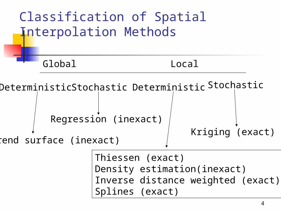
Classification of Spatial Interpolation Methods

Global

Deterministic Stochastic

Local

Deterministic Stochastic

Thiessen (exact)Density estimation(inexact)Inverse distance weighted (exact)Splines (exact)

Kriging (exact)Regression (inexact)

Trend surface (inexact)

5

Global Interpolation Global use all available data to provide

predictions for the whole area of interest, while local interpolations operate within a small zone around the point being interpolated to ensure that estimates are made only with data from locations in the immediate neighborhood.

Two types of global: Trend surface and regression methods

6

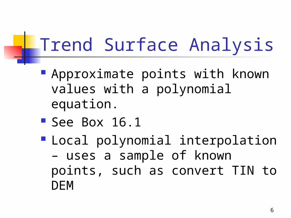
Trend Surface Analysis Approximate points with known

values with a polynomial equation. See Box 16.1 Local polynomial interpolation –

uses a sample of known points, such as convert TIN to DEM

7

Local, deterministic methods

Define an area around the point

Find data point within neighborhood

Choose model

Evaluate point value

8

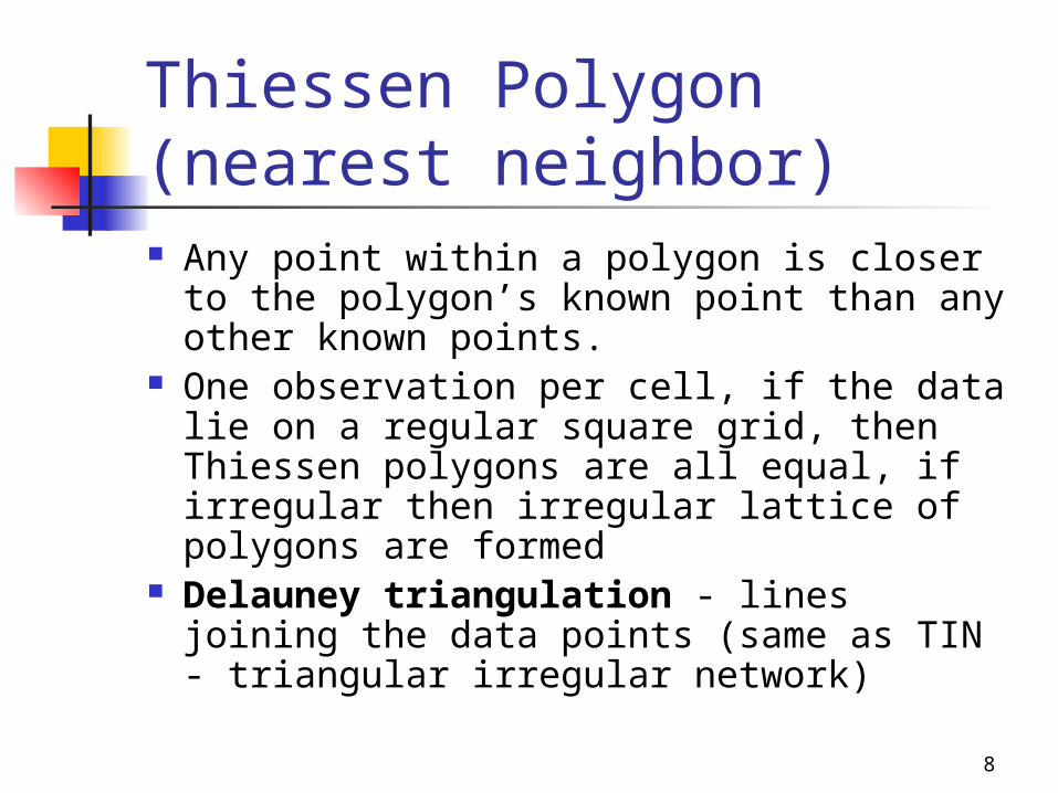
Thiessen Polygon (nearest neighbor) Any point within a polygon is closer to

the polygon’s known point than any other known points.

One observation per cell, if the data lie on a regular square grid, then Thiessen polygons are all equal, if irregular then irregular lattice of polygons are formed

Delauney triangulation - lines joining the data points (same as TIN - triangular irregular network)

9

Thiessen polygons

Delauney Triangulation

10

Example data set soil data from Mass near the village of

Stein in the south of the Netherlands all point data refer to a support of

10x10 m, the are within which bulked samples were collected using a stratified random sampling scheme

Heavy metal concentration measured

11

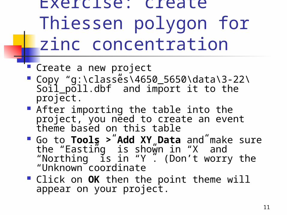
Exercise: create Thiessen polygon for zinc concentration

Create a new project Copy “g:\classes\4650_5650\data\3-22\

Soil_poll.dbf” and import it to the project. After importing the table into the project,

you need to create an event theme based on this table

Go to Tools > Add XY Data and make sure the “Easting” is shown in “X” and “Northing” is in “Y”. (Don’t worry the “Unknown coordinate”

Click on OK then the point theme will appear on your project.

12

This is what you might see on screen

13

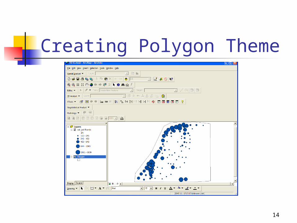
Create a polygon theme The next thing you need to do is

provide the Thiessen polygon a boundary so that the computing of irregular polygons can be reasonable

Use ArcCatalog to create a new shapefile and name it as “Polygon.shp”

Add this layer to your current project. Use “Editor” to create a polygon.

14

Creating Polygon Theme

15

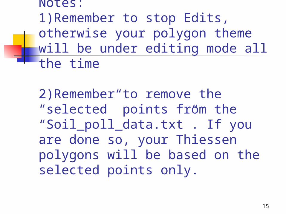
Notes: 1)Remember to stop Edits, otherwise your polygon theme will be under editing mode all the time

2)Remember to remove the “selected” points from the “Soil_poll_data.txt”. If you are done so, your Thiessen polygons will be based on the selected points only.

16

Extent and Cell Size

Go to “Spatial Analyst > Options” and click on tab and use “Polygon” as the “Analysis Mask”.

If the Analysis Mask is not set, the output layer will have rectangular shape.

17

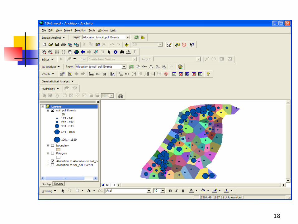
Thiessen Polygon from Spatial Analyst

Select Spatial Analyst > Distance > Allocation.

In “Assign to”, select “soil_poll Event” and

Change the default cell size to “0.1”

click OK to create cell in temporary folder.

18

19

Join Tables Join soil_poll Events

to Alloc3 grid file by “ObjectID” in Alloc3 and “OID” in soil_poll Events.

Click “Advanced” button. Two options are available for joining tables.

Open Attribute of “Alloc3” (name may vary) and view the joined fields.

20

Zinc Concentration

Symbolize the grid with two-color ramp based on Zn concentration

21

Density Estimation Simple method – divide total point

value by the cell size Kernel estimation – associate each

known point with a kernel function, a probability density function.

22

Exercise Compute density of the

sampling points from previous dataset.

If you use the xy-event points for calculation, you might receive error message.

Convert this layer to shape file before using Density function from Spatial Analyst.

Select your cell size (such as 1,) and search radius as 5.

23

Density function output

24

Inverse Distance Weighted the value of an attribute z at some

unsampled point is a distance-weighted average of data point occurring within a neighborhood, which compute:

ki

n

ki

n

i

d

dZZ

/1

/

1

1

Z =estimated value at an unsampled point

n= number of control points used to estimate a grid point

k=power to which distance is raised

d=distances from each control points to an unsampled point

25

Computing IDW

2 4 6 X

6

4

2

Z1=40

Z2=60

Z4=40Z3=50

24.25 41.12

Do you get 49.5 for the red square?

ki

n

ki

n

i

d

dZZ

/1

/

1

1

Use k = 1

26

Exercise - generate a Inversion distance weighting surface and contour

Spatial Analyst > Interpolate to Raster > Inverse Distance Weighted

Make sure you have set the Output cell size to 0.1

27

Contouring create a contour

based on the surface from IDW

28

IDW and Contouring

29

Problem - solution Unsampled point may have a higher data value

than all other controlled points but not attainable due to the nature of weighted average: an average of values cannot be lesser or greater than any input values - solution:

Fit a trend surface to a set of control points surrounding an unsampled point

Insert X and Y coordinates for the unsampled point into the trend surface equation to estimate a value at that point

30

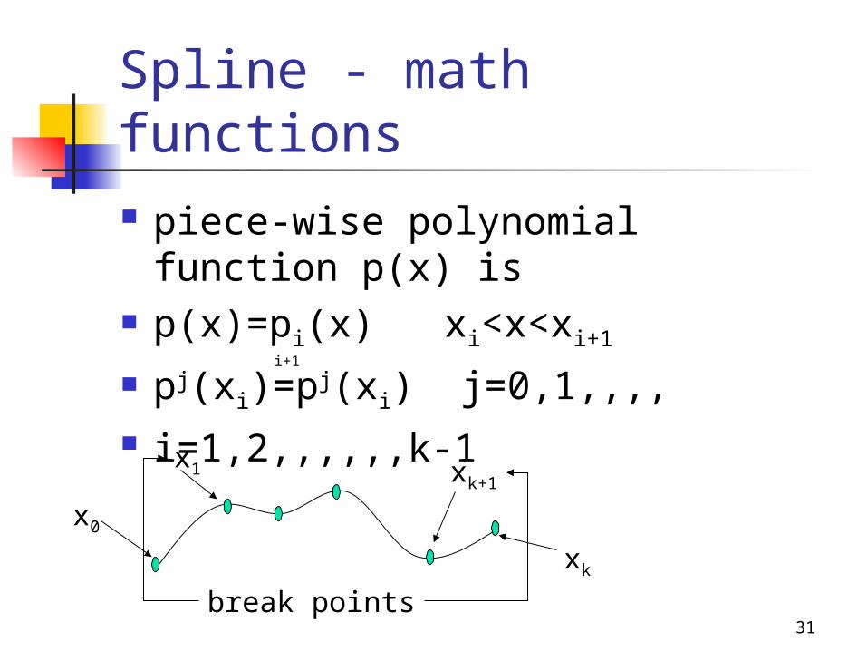
Splines draughtsmen used flexible rulers

to trace the curves by eye. The flexible rulers were called “splines” - mathematical equivalents - localized

piece-wise polynomial function p(x) is

31

Spline - math functions piece-wise polynomial function

p(x) is p(x)=pi(x) xi<x<xi+1

pj(xi)=pj(xi) j=0,1,,,, i=1,2,,,,,,k-1

i+1

x0

xk

x1 xk+1

break points

32

Spline r is used to denote the constraints

on the spline (the functions pi(x) are polynomials of degree m or less

r = 0 - no constraints on function

33

Exercise: create surface from spline have point data theme activated select “Surface > Interpolate Grid Define the output area and other

parameters Select “Spline” in Method field,

“Zn” for Z Value Field and “regularized” as type

34

Kriging Comes from Daniel Krige, who

developed the method for geological mining applications

Rather than considering distances to control points independently of one another, kriging considers the spatial autocorrelation in the data

35

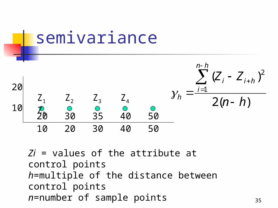
semivariance

10 20 30 40 50

20

10Z1 Z2 Z3 Z4

Z520 30 35 40 50)(2

)(1

2

hn

ZZhn

ihii

h

Zi = values of the attribute at control pointsh=multiple of the distance between control pointsn=number of sample points

36

Semivariance

hh=1, h=2 h=3 h=4

21.88 91.67 156.25 312.50

(Z1-Z1+h)2

(Z2-Z2+h)2

(Z3-Z3+h)2

(Z4-Z4+h)2

sum2(n-h)

1002525251758

225100100

4256

400225

6254

625

6252

)(2

)(1

2

hn

ZZhn

ihii

h

37

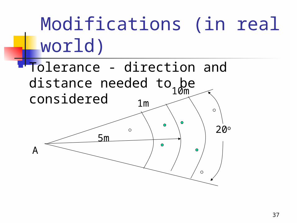
Modifications (in real world)

Tolerance - direction and distance needed to be considered

5m

1m10m

20o

A

38

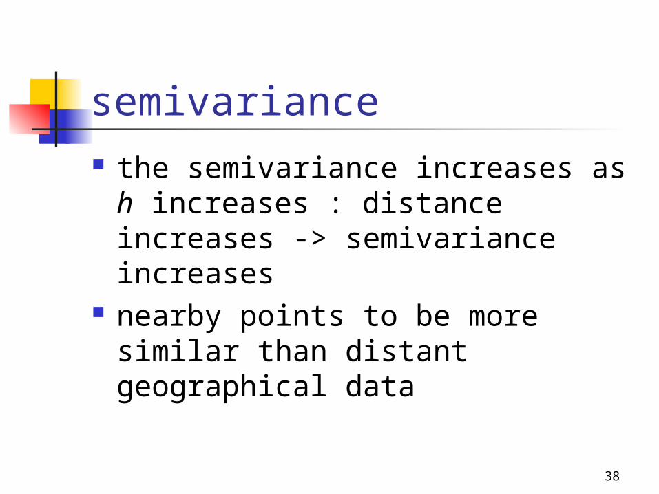
semivariance the semivariance increases as h

increases : distance increases -> semivariance increases

nearby points to be more similar than distant geographical data

39

data no longer similar to nearby values

h

h

sill

range

40

kriging computations we use 3 points to estimate a grid

point again, we use weighted average

Z =w1Z1 + w2Z2+w3Z3

Z= estimated value at a grid point

Z1,Z2 and Z3 = data values at the control pointsw1,w2, and w3 = weighs associated with each control point

41

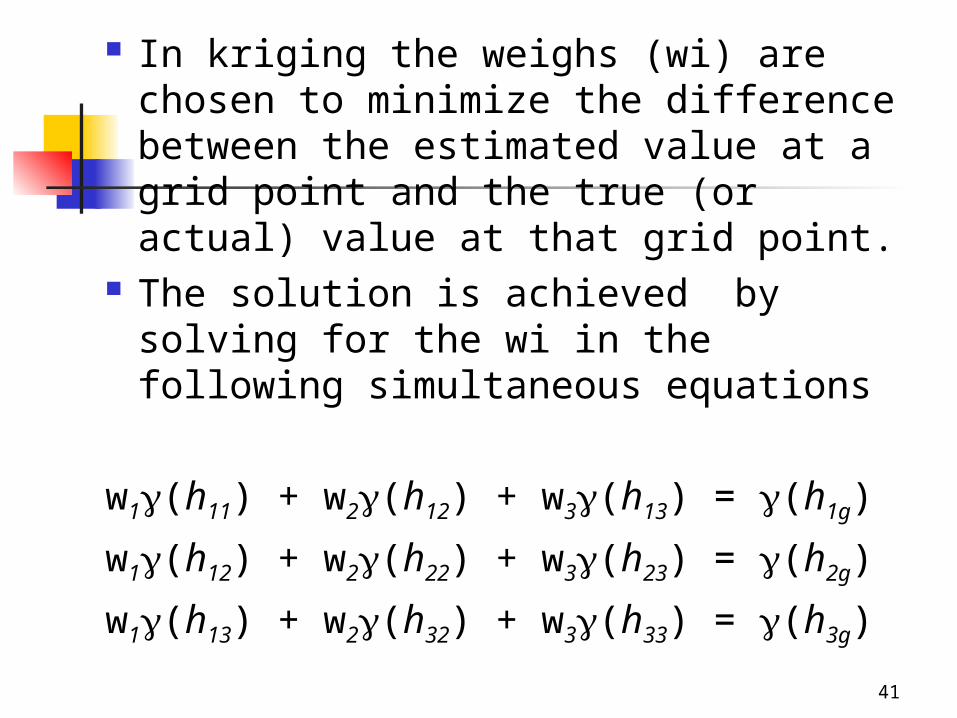
In kriging the weighs (wi) are chosen to minimize the difference between the estimated value at a grid point and the true (or actual) value at that grid point.

The solution is achieved by solving for the wi in the following simultaneous equations

w1(h11) + w2(h12) + w3(h13) = (h1g)

w1(h12) + w2(h22) + w3(h23) = (h2g)

w1(h13) + w2(h32) + w3(h33) = (h3g)

42

w1(h11) + w2(h12) + w3(h13) = (h1g)

w1(h12) + w2(h22) + w3(h23) = (h2g)

w1(h13) + w2(h32) + w3(h33) = (h3g)

Where (hij)=semivariance associated with distance bet/w control points i and j.

(hig) =the semivariance associated with the distance bet/w ith control point and a grid point.

Difference to IDW which only consider distance bet/w the grid point and control points, kriging take into account the variance between control points too.

43

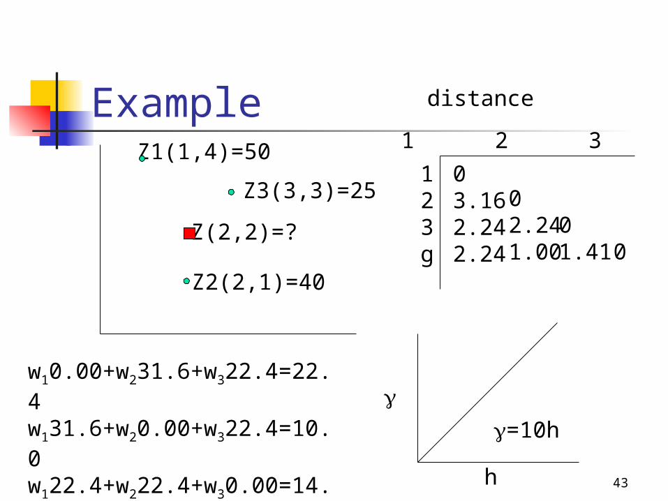
ExampleZ1(1,4)=50

Z2(2,1)=40

Z3(3,3)=25

Z(2,2)=?

1 2 3 g

03.162.242.24

02.241.00

01.410

123g

distance

h

=10h

w10.00+w231.6+w322.4=22.4w131.6+w20.00+w322.4=10.0w122.4+w222.4+w30.00=14.1

44

=0.15(50)+0.55(40) + 0.30(25) = 37

Z

45

Homework 6 – due next Thursday midnight.

Task 1: Chapter 16 tasks Task 2:

Calculate volume of contaminated Pb soil in Thiessen polygon exercise based on range of every 50 ppm, assuming soil density of 1.65 g/cm3 and only the top 1-foot soil is considered.

Use IDW to compute the volume of the contaminated Pb

Use Kriging (if it’s working) to compute concentration of Pb

Compare these three methods and see the differences (use same output cell size for all three methods)

In Doc file, describe your selection of cell size, search radius and results from different choice of cell sizes (if you have time to create layers with different cell sizes.