journal of hydrology - everglades-hub10jhydrol-71-lomods… · assistance of ercan kahya, associate...

Journal of Hydrology 387 (2010) 165–175

Contents lists available at ScienceDirect

Journal of Hydrology

journal homepage: www.elsevier .com/ locate / jhydrol

Triple diagram models for prediction of suspended solid concentration in LakeOkeechobee, Florida

Abdüsselam Altunkaynak a,b,*, Keh-Han Wang b

a Faculty of Civil Engineering, Hydraulics, Division, Istanbul Technical Univ., Maslak 34469, Istanbul, Turkeyb Department of Civil and Environmental Engineering, University of Houston, 4800 Calhoun, Houston, TX 77204-4003, United States

a r t i c l e i n f o

Article history:Received 26 November 2009Received in revised form 10 March 2010Accepted 29 March 2010

This manuscript was handled byDr. A. Bardossy, Editor-in-Chief, with theassistance of Ercan Kahya, Associate Editor

Keywords:Contour mapPredictionKriging optimum interpolation techniqueLake OkeechobeeSediment/water interactionModel

0022-1694/$ - see front matter � 2010 Elsevier B.V. Adoi:10.1016/j.jhydrol.2010.03.035

* Corresponding author at: Department of Civil andUniversity of Houston, 4800 Calhoun, Houston, TX 77

E-mail addresses: [email protected], aaltunka@[email protected] (K.-H. Wang).

s u m m a r y

Lake Okeechobee in Florida is a major component of the greater Everglades hydrologic system and pro-vides a number of valuable uses to society and nature, such as water supply, navigation, wildlife habitat,and fishery. Suspended solid concentration (SSC) affects directly the lake’s conditions for some of theseapplications. Therefore, accurate prediction of SSC can enhance the management of the water qualityand the long-term protection of Lake Okeechobee. Extensive data, including wind speed, flow velocity,flow direction and SSC, have been collected. Models for predicting suspended solid concentration basedon 10 different scenarios are developed using these measurements. Data are divided into two groups astraining and testing for the construction of the models. SSC is predicted by the Kriging interpolation tech-nique. Criterions of mean relative error, root mean squared error and coefficient of efficiency (CE) areused to determine the prediction errors of the developed models. In general, mean relative error is below7% and coefficient of efficiency stays above 0.92 for the models presented. Graphs, results, and interpre-tations are given in detail in this paper.

� 2010 Elsevier B.V. All rights reserved.

1. Introduction

Lake Okeechobee is one of the most important water bodies inthe state of Florida for the use of different purposes such as, watersupply, navigation, wildlife habitat and commercial fishery. Thelake, located in south-central Florida, covers a surface area of1730 km2 with an average depth of 2.7 m (South Florida WaterManagement District (SFWMD), 2007). Considering its huge stor-age capacity as the largest lake in the southeastern United States,Lake Okeechobee also serves important hydrologic and ecologicroles for the region of great Everglades in Florida.

Wind has a dominant effect on the motion and mixing of waterin shallow water bodies. In Lake Okeechobee flow circulation,free-surface oscillation, and transportation of the sediments areattributable to wind blowing over the lake (Wang et al., 2003). Amodeling study of wind induced sediment resuspension in a shal-low estuary by Liu and Huang (2009) also confirmed the strongcorrelation between wind and the transport of suspended sedi-ments. The bottom sediments in Lake Okeechobee contain a largearea of semi-fluid mud. Resuspended sediment is a major concern

ll rights reserved.

Environmental Engineering,204-4003, United States.ail.uh.edu (A. Altunkaynak),

in Lake Okeechobee. Sediment resuspension causes greater turbid-ity and reducing light penetration through the water column. It isalso noticeable that the internal phosphorus loads associated withresuspended sediments are approximately the same order of mag-nitude as the external loads (Reddy 1991). By examining the phos-phorous budgets of Lake Okeechobee, for around 10 years span of1990th, the phosphorous has accumulated in the sediments atthe rate of 303 metric tons per year (Reedy et al. 2002). Therefore,over the decades through excessive phosphorus (P) loading andaccumulation of fine sediments, there is an increasing concern thatthe increase of suspended sediments may be impacting the waterquality of the lake.

An extensive field study on Lake Okeechobee has been carriedout by Wang et al. (2003) to collect time varying hydrodynamicdata including three-dimensional flow velocities and suspendedsolid concentrations. The effects of wind and flow velocities ontransporting SSC were analyzed statistically. Currently, a Lake Oke-echobee Environmental Model (LOEM) has been applied to predictwater circulation patterns and suspended solid concentration (SSC)(Jin et al., 2002; Jin and Ji, 2004). However, it would be interestingand practical to establish other pretictive models that can providemore effective and accurate estimation on SSC for the impact studyof the Lake Okeechobee.

The Triple Diagram Model (TDM), firstly proposed by Altunkay-nak and his colleagues in 2003, concurrently shows the variation of

http://dx.doi.org/10.1016/j.jhydrol.2010.03.035

mailto:[email protected]



http://www.sciencedirect.com/science/journal/00221694

http://www.elsevier.com/locate/jhydrol

166 A. Altunkaynak, K.-H. Wang / Journal of Hydrology 387 (2010) 165–175

three variables and can be used for predictions (Altunkaynak et al.,2003; S�en et al., 2004). Also, plots obtained by this technique facil-itate the procedure of making useful explanations of the influencingtrend among variables. To establish the TDM, three variables,including two affecting variables, and one dependent variable, arerequired. In this study, 10 TDMs are developed with the applicationof the constructed contour maps of three variables to identify andrelate the effects of wind speed (WS), surface flow velocity (FV),and flow direction (FD) to SSC and the classical Kriging technique,or the so called geostatistical approach, (Matheron, 1963) to deter-mine the time variation of SSC at a station in Lake Okeechobee.

2. Kriging approach

The principal of the Kriging (optimum interpolation) approachis to establish a valid variogram model that can interpret and char-acterize the structural relationships of natural phenomenon. Inother words, the variogram model can be used as a simple and reli-able statistical tool to interpret the regional behaviour of a randomfield. The Kriging method (Krige, 1951) has been adopted for appli-cations in various areas, such as earth sciences (Journel andHuijbregts, 1978; Isaaks and Srivastava, 1989; Cressie, 1993), min-ing (Matias et al., 2004), tunnels (Öztürk and Nasuf, 2002), oceanengineering (Altunkaynak, 2005; Ozger and Sen, 2007) and hydrol-ogy (Altunkaynak, 2009; Altunkaynak et al., 2003; S�en et al., 2004).In this study, a series of SSC related contour maps are prepared byusing the geostatistical approach for the development of predictionmodels for SSC in the water column of the Lake Okeechobee.

One of the major principles of the geostatistical applications isto describe the behaviour of a natural phenomenon relying ontwo different variables. For the present Lake Okeechobee study,variables such as wind speed, flow velocity, and flow directioncan be paired as two input location variables for the predictionof SSC as regional variable (ReV). For example, SSC contour mapscan be constructed with the variables of wind speed and flowvelocity using Kriging approach. Other contour maps with selec-tion of two other input variables can also be obtained. Overall, thismapping technique is adopted to facilitate the understanding ofthe alteration of current SSC with the effects of wind speed, flowvelocity, flow direction, and previous SSC. It is also applied to showthe relationships between the surface SSC with the middle-layerSSC or the bottom-layer SSC.

Regional dependency between scattered points can be definedby the following equation (Matheron, 1963; Journel andHuijbregts, 1978; Isaaks and Srivastava, 1989; S�en 1989),

cðdÞ ¼ 12NðdÞ

XNðdÞi¼1

½Cðxþ dÞ � CðxÞ�2 ð1Þ

This expression is called semivariogram (SV) function. Here,c(d) = SV function; N(d) = number of pairs of two variables for dis-tance d; C(x) = magnitude of the regional variable; andC(x + d) = magnitude of the regional variable that is away fromthe C(x) by a distance d. For example, when the wind speed andflow velocity are considered as the independent variables and theSSC as the dependent variable, the distances are calculated be-tween data points formed by the wind speed and flow velocity.Generally, a geostatistical study covers two steps: (i) obtainingsemivariogram and (ii) solving the prediction problem using theKriging. The fundamental procedure of a Kriging system is to min-imize the error variance (Isaaks and Srivastava, 1989; Subyani1997; Altunkaynak et al. 2003; S�en et al., 2004). The followingequation can be used for the SSC prediction at any point of the con-tour map,

CðxoÞ ¼XN

i¼1

wi CðxiÞ: ð2Þ

Here, C(xo) = magnitude of the SSC at any prediction point xo;C(xi) = SSC measurements at point i; and wi = weighting coefficientsthat can be determined by solving the following system of equa-tions constructed from the semivariogram function (Isaaks andSrivastava, 1989; Subyani, 1997)

w1

w2

�wn

l

26666664

37777775¼

c11 c12 � c1n 1c21 c22 � c2n 1� � � � �

cn1 cn2 � cnn 11 1 1 1 0

26666664

37777775

�1 c1o

c2o

��

cno

1

2666666664

3777777775

ð3Þ

Here cij = values of semivariogram between two points, namely, iand j; cio = values of semivariogram between point i and the predic-tion point o; and l = Lagrange parameter. Therefore, the weightingmatrix can be obtained from two variables (e.g. a combination oftwo variables selected from wind speed, flow velocity, flow direc-tion, and SSC at previous time level) by applying various scenariosof the variables for the development of predictive models for esti-mating the surface-layer SSC or SSC at middle or bottom layer.

3. Study area and sources of data

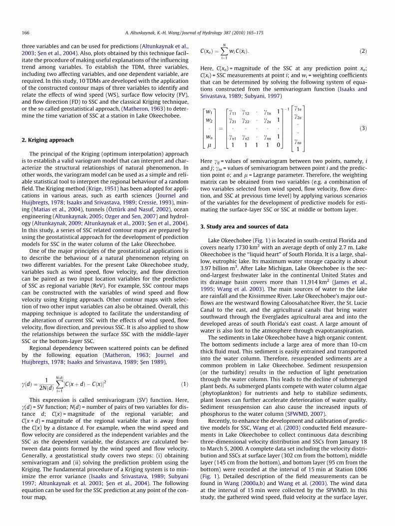
Lake Okeechobee (Fig. 1) is located in south-central Florida andcovers nearly 1730 km2 with an average depth of only 2.7 m. LakeOkeechobee is the ‘‘liquid heart” of South Florida. It is a large, shal-low, eutrophic lake. Its maximum water storage capacity is about3.97 billion m3. After Lake Michigan, Lake Okeechobee is the sec-ond-largest freshwater lake in the continental United States andits drainage basin covers more than 11,914 km2 (James et al.,1995; Wang et al. 2003). The main sources of water to the lakeare rainfall and the Kissimmee River. Lake Okeechobee’s major out-flows are the westward flowing Caloosahatchee River, the St. LucieCanal to the east, and the agricultural canals that bring watersouthward through the Everglades agricultural area and into thedeveloped areas of south Florida’s east coast. A large amount ofwater is also lost to the atmosphere through evapotranspiration.

The sediments in Lake Okeechobee have a high organic content.The bottom sediments include a large area of more than 10-cmthick fluid mud. This sediment is easily entrained and transportedinto the water column. Therefore, resuspended sediments are acommon problem in Lake Okeechobee. Sediment resuspension(or the turbidity) results in the reduction of light penetrationthrough the water column. This leads to the decline of submergedplant beds. As submerged plants compete with water column algae(phytoplankton) for nutrients and help to stabilize sediments,plant losses can further accelerate deterioration of water quality.Sediment resuspension can also cause the increased inputs ofphosphorus to the water column (SFWMD, 2007).

Recently, to enhance the development and calibration of predic-tive models for SSC, Wang et al. (2003) conducted field measure-ments in Lake Okeechobee to collect continuous data describingthree-dimensional velocity distribution and SSCs from January 18to March 5, 2000. A complete data set including the velocity distri-bution and SSCs at surface layer (302 cm from the bottom), middlelayer (145 cm from the bottom), and bottom layer (95 cm from thebottom) were recorded at the interval of 15 min at Station L006(Fig. 1). Detailed description of the field measurements can befound in Wang (2000a,b) and Wang et al. (2003). The wind dataat the interval of 15 min were collected by the SFWMD. In thisstudy, the gathered wind speed, fluid velocity at the surface layer,

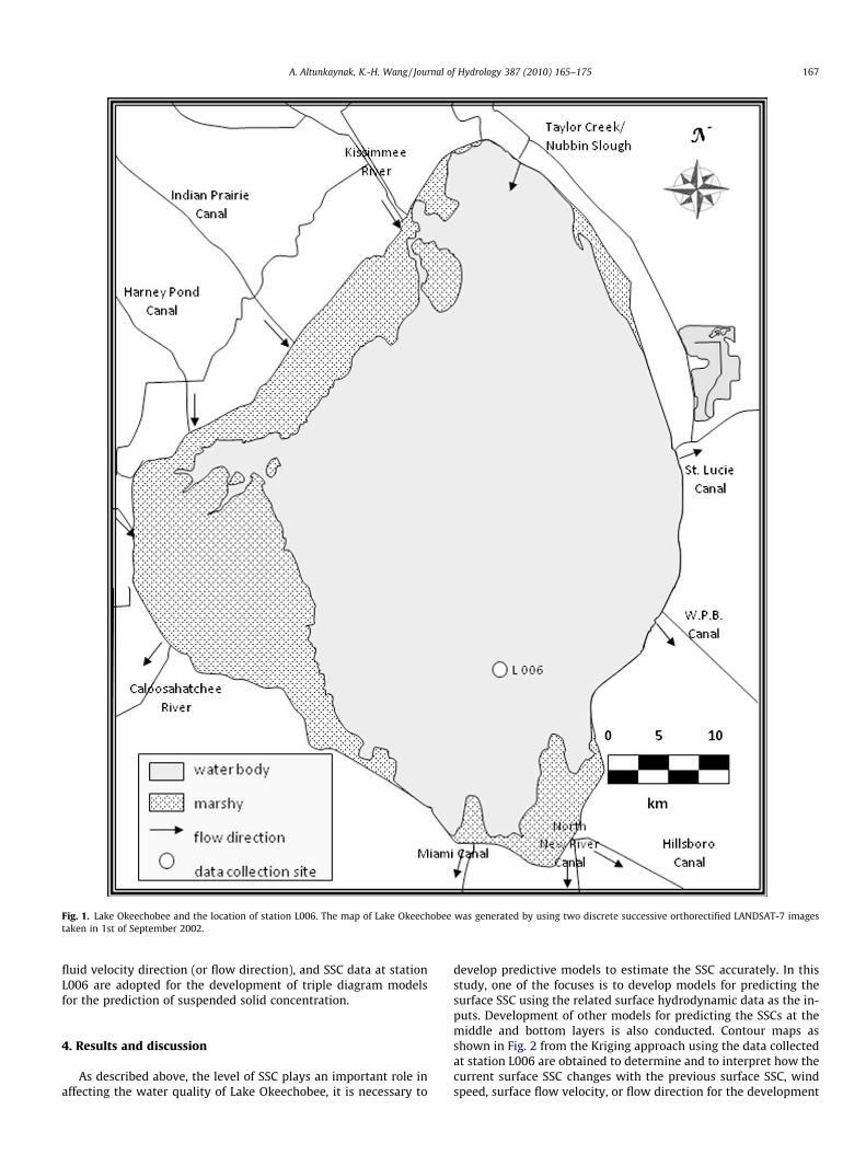
Fig. 1. Lake Okeechobee and the location of station L006. The map of Lake Okeechobee was generated by using two discrete successive orthorectified LANDSAT-7 imagestaken in 1st of September 2002.

A. Altunkaynak, K.-H. Wang / Journal of Hydrology 387 (2010) 165–175 167

fluid velocity direction (or flow direction), and SSC data at stationL006 are adopted for the development of triple diagram modelsfor the prediction of suspended solid concentration.

4. Results and discussion

As described above, the level of SSC plays an important role inaffecting the water quality of Lake Okeechobee, it is necessary to

develop predictive models to estimate the SSC accurately. In thisstudy, one of the focuses is to develop models for predicting thesurface SSC using the related surface hydrodynamic data as the in-puts. Development of other models for predicting the SSCs at themiddle and bottom layers is also conducted. Contour maps asshown in Fig. 2 from the Kriging approach using the data collectedat station L006 are obtained to determine and to interpret how thecurrent surface SSC changes with the previous surface SSC, windspeed, surface flow velocity, or flow direction for the development


of predictive models. Presented in Figs. 3 and 4 are the contourmaps used to develop models that predict the values of middle-layer SSC and bottom-layer SSC from the inputs of surface SSC.As we know obtaining the measurements at the surface level are

Fig. 2. Surface suspended solid concentration (SSC) conto

generally easier than the middle or bottom level. Therefore, inprinciple, only limited efforts are needed to collect the data of sur-face SSC as the SSC at the other layers can be predicted from thecalibrated models. In this study, we establish and test 10 TDMs

ur maps using: (a) Model 1, (b) Model 2, (c) Model 3.

Fig. 3. Middle-layer suspended solid concentration (SSC) contour maps using: (a) Model 4, (b) Model 5, (c) Model 6.


for predicting the current SSC at L006 based on the current (timestep k) or previous (time step k � 1) data of affecting variables.Data are divided into two groups; one group with 3500 data points

is for the training (or calibration) and the other group with theremaining 1000 data points is for the prediction (testing or valida-tion). Contour maps of Models 1–10 are given in Figs. 2–5. Details

Fig. 4. Bottom-layer suspended solid concentration (SSC) contour maps using: (a) Model 7, (b) Model 8, (c) Model 9.


of these models with the selections of the input and output vari-ables as well as the analyzed errors are summarized in Table 1.

Considering the important effect of previous surface SSC on theprediction of current surface SSC (at k time level), the basic models

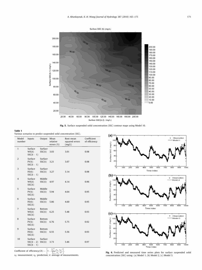
Fig. 5. Surface suspended solid concentration (SSC) contour maps using Model 10.

Table 1Various scenarios to predict suspended solid concentration (SSC).

Modelnumber

Inputs Output Meanrelativeerrors (%)

Root meansquared errors(mg/L)

Coefficientof efficiency

1 Surface SurfaceWS(k) SSC(k) 3.03 3.01 0.98SSC(k � 1)

2 Surface SurfaceFV(k) SSC(k) 3.21 3.07 0.98SSC(k � 1)

3 Surface SurfaceFD(k) SSC(k) 3.27 3.14 0.98SSC(k � 1)

4 Surface MiddleWS(k) SSC(k) 4.97 4.14 0.96SSC(k)

5 Surface MiddleFV(k) SSC(k) 5.94 4.64 0.95SSC(k)

6 Surface MiddleFD(k) SSC(k) 5.86 4.60 0.95SSC(k)

7 Surface BottomWS(k) SSC(k) 6.25 5.48 0.93SSC(k)

8 Surface BottomFV(k) SSC(k) 6.76 5.75 0.92SSC(k)

9 Surface BottomFD(k) SSC(k) 6.55 5.56 0.93SSC(k)

10 Surface SurfaceSSC(k � 2) SSC(k) 3.73 3.46 0.97SSC(k � 1)

Coefficient of efficiencyðCEÞ ¼ 1�PN

i¼1ðxoi�xpi

Þ2PN

i¼1ðxoi�xÞ2

� �.

xo: measurement; xp: prediction; x: average of measurements.Fig. 6. Predicted and measured time series plots for surface suspended solidconcentration (SSC) using: (a) Model 1, (b) Model 2, (c) Model 3.



based on the inputs of the previous surface SSC (at k � 1 time level)and one of the chosen variables from wind speed, flow velocity,and flow direction are developed respectively as Model 1, Model2, and Model 3 (see Table 1). In addition, the Model 10 can be usedto predict the current surface SSC using surface SSC data from twoprevious time levels (i.e. k � 1 and k � 2 time levels) at occasionsthe data of wind speed, flow velocity, and flow direction are notavailable. For the SSC at other layers, we also develop six models(named as Model 4, Model 5, Model 6, Model 7, Model 8, and Mod-el 9) to predict the SSC values at middle and bottom layers usingonly inputs from surface data.

For the Model 1 with inputs of previous SSC and wind speed, theKriging contour map shown in Fig. 2a demonstrates the strongrelationship between SSC(k � 1) (k � 1 time level) and SSC(k) (ktime level or current time level). Contour results generally can bedivided into three different sets as Low, Medium, and High. WhenSSC(k � 1) increases, SSC(k) increases. It is also shown that whenwind speed(k) is High, SSC(k) is High. When wind speed(k) isLow or Medium, SSC(k) is Low or Medium, respectively. These rulesare similar to those proposed in the fuzzy logic sets by Zadeh(1965). This contour plot shows the positive correlations betweenthese variables.

Examining the effect of current flow velocity on the surface SSCas considered in Model 2, we notice from Fig. 2b that no apparentpositive correlation between flow velocity(k) and SSC(k) can beconcluded. An increase in SSC is seen in lower flow velocity values.This may be a combined result of sediment settling and reducedsediments transported out from the station L006. The data reveal-ing the transport of sediment from a certain flow direction to

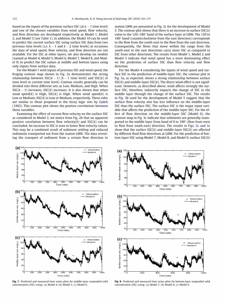
Fig. 7. Predicted and measured time series plots for middle-layer suspended solidconcentration (SSC) using: (a) Model 4, (b) Model 5, (c) Model 6.

station L006 are presented in Fig. 2c for the development of Model3. The contour plot shows that there is an increase in surface SSC(k)value in the 120–180� band of the surface layer at L006. The 120 to180� band (counterclockwise from the east direction) correspondsto the flow from the south-east to the flow from the east direction.Consequently, the flows that move within the range from thesouth-east to the east directions carry more SSC as compared toSSC from other directions. The results from Model 1, Model 2 andModel 3 indicate that wind speed has a more dominating effecton the prediction of surface SSC than flow velocity and flowdirection.

For the Model 4 considering the inputs of wind speed and sur-face SSC to the prediction of middle-layer SSC, the contour plot inFig. 3a, as expected, shows a strong relationship between surfaceSSC(k) and middle-layer SSC(k). The direct wind effect is not signif-icant. However, as described above, wind affects strongly the sur-face SSC, therefore, indirectly impacts the change of SSC in themiddle layer through the change of the surface SSC. The resultsin Fig. 3b used for the development of Model 5 suggest that thesurface flow velocity also has less influence on the middle-layerSSC than the surface SSC. The surface SSC is the major input vari-able that affects the prediction of the middle-layer SSC. For the ef-fect of flow direction on the middle-layer SSC (Model 6), thecontour map in Fig. 3c indicate that sediments are generally trans-ported to the middle layer from band of 0 to 100� (flow from westto flow from south-east) direction. The results in Figs. 2c and 3cshow that the surface SSC(k) and middle-layer SSC(k) are affectedby different fluid flow directions at L006. For the prediction of bot-tom-layer SSC using Model 7, Model 8, and Model 9, surface SSC(k)

Fig. 8. Predicted and measured time series plots for bottom-layer suspended solidconcentration (SSC) using: (a) Model 7, (b) Model 8, (c) Model 9.


is again revealed to have a greater contribution to the bottom-layerSSC(k) as shown in Fig. 4a–c. The surface flow velocity is not shownto have strong correlation with the bottom-layer SSC. For the effectof the flow direction, the contour plot in Fig. 4c shows that the bot-tom-layer SSC(k) is affected mostly by the south-east flow tonorth-east flow (150–230�).

A Contour map for Model 10 is constructed in Fig. 5 using thesurface SSC(k) and two previous surface SSCs, i.e. SSC(k � 2) andSSC(k � 1). This map shows obviously that there is a strong rela-tionship among the data of surface SSC(k), SSC(k � 1), andSSC(k � 2). Also, while the values of surface SSC(k � 2) andSSC(k � 1) increase, surface SSC(k) increases. This indicates thatthe autocorrelation of SSC(k) either with lag-1 data of SSC(k � 1)or with lag-2 data of SSC(k � 2) is strong.

The time series plots showing the comparisons of measuredsurface SSCs and the predicted values using Model 1, Model 2,and Model 3 for the data set selected for prediction are pre-sented in Fig. 6a–c, respectively. The time series data selectedfor prediction include 1000 data points and the time indexshown along the horizontal coordinate represents time with eachunit being equal to 15 min. From Fig. 6a–c, it is noted that thepredicted values follow the recorded data with great consistency.Mean relative error is 3.03% and root mean squared error is3 mg/L for Model 1. Also, the coefficient of efficiency, CE, show-ing the consistency between measured and predicted data, is0.98. The CE is defined as CE = 1�(mean square errors/varianceof observation). The good agreement between observation andprediction for Model 1 is also demonstrated in Fig. 10a with aplot of predicted surface SSCs with measured data followingthe 45� perfect model line.

The results obtained by using the Model 2 give respectivelythe mean relative error, root mean squared error, and coefficientof efficiency as 3.21%, 3.07 mg/L and 0.98. The consistency be-tween observation and prediction is also shown to follow the per-fect model line in Fig. 10b. When Model 3 is applied, the values ofmean relative error, root mean squared error, and coefficient ofefficiency are respectively 3.37%, 3.14 mg/L, and 0.98, similar tothe results computed from Model 1 and Model 2. The trend ofagreement between observation and prediction for Model 3 isshown in Fig. 10c. Although each model among Models 1, 2,and 3 produces similar predictions, slightly enhanced scatteringdata along the 45� line are shown in Fig. 10b and c when com-pared to the data plot in Fig. 10a. This further confirms that thecorrelation of SSC(k) and wind speed(k) is greater than the corre-lation between SSC(k) and flow velocity(k) or flow direction(k).Considering the convenience of the inputs of the affecting vari-ables and the accuracy of the model prediction, Model 1 can beserved as a practical and effective model for estimating surfaceSSC.

Fig. 9. Predicted and measured time series plots for surface suspended solidconcentration (SSC) using Model 10.

In principle, measurements in the middle and bottom layers arerelatively difficult and not cost-effective when compared to thesurface measurements. Extending the measurements of surfaceSSC to predict middle or bottom-layer SSC can be practicallyimportant. Models 4–6 are developed to predict the middle-layerSSC(k) and Models 7–9 can be used to predict the bottom-layerSSC(k) by using wind speed(k), flow velocity(k), flow direction(k),and surface SSC(k) as inputs. For the estimation of middle-layerSSC, the predicted time series results using Model 4, Model 5,and Model 6 are given in Fig. 7a–c, respectively, whereas the cor-responding perfect model line plots are shown in Fig. 11a–c. Thecomparison plots for the predicted bottom-layer SSCs using Model7, Model 8, and Model 9 are shown respectively in Fig. 8a–c and inFig. 12a–c. Examining the results shown in Figs. 7 and 8, it is notedthat the middle-layer SSC(k) can be predicted with less error thanthe bottom-layer SSC(k). Greater deviations, when comparing tothe recorded data, are noticed in predicted values in Fig. 8 thanthose in Fig. 7. In general, predictions of middle-layer SSC(k) and

Fig. 10. Comparisons of observed and predicted surface suspended solid concen-tration (SSC) using: (a) Model 1, (b) Model 2, (c) Model 3.

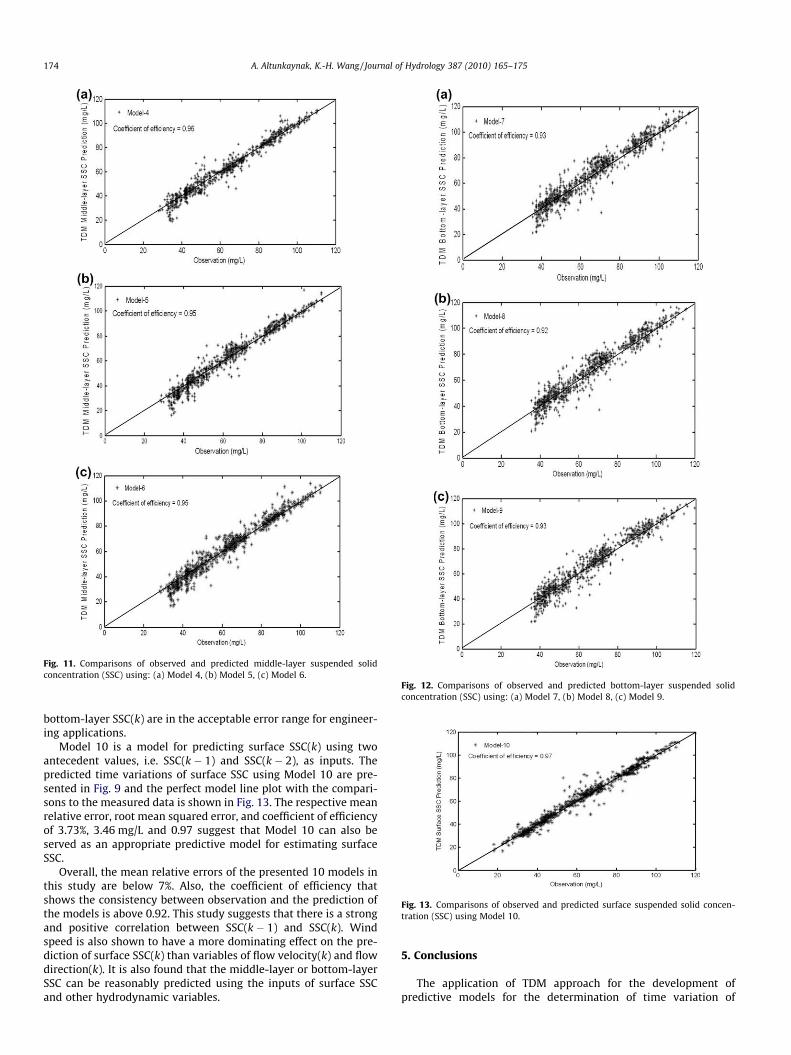
Fig. 11. Comparisons of observed and predicted middle-layer suspended solidconcentration (SSC) using: (a) Model 4, (b) Model 5, (c) Model 6.

Fig. 12. Comparisons of observed and predicted bottom-layer suspended solidconcentration (SSC) using: (a) Model 7, (b) Model 8, (c) Model 9.

Fig. 13. Comparisons of observed and predicted surface suspended solid concen-tration (SSC) using Model 10.


bottom-layer SSC(k) are in the acceptable error range for engineer-ing applications.

Model 10 is a model for predicting surface SSC(k) using twoantecedent values, i.e. SSC(k � 1) and SSC(k � 2), as inputs. Thepredicted time variations of surface SSC using Model 10 are pre-sented in Fig. 9 and the perfect model line plot with the compari-sons to the measured data is shown in Fig. 13. The respective meanrelative error, root mean squared error, and coefficient of efficiencyof 3.73%, 3.46 mg/L and 0.97 suggest that Model 10 can also beserved as an appropriate predictive model for estimating surfaceSSC.

Overall, the mean relative errors of the presented 10 models inthis study are below 7%. Also, the coefficient of efficiency thatshows the consistency between observation and the prediction ofthe models is above 0.92. This study suggests that there is a strongand positive correlation between SSC(k � 1) and SSC(k). Windspeed is also shown to have a more dominating effect on the pre-diction of surface SSC(k) than variables of flow velocity(k) and flowdirection(k). It is also found that the middle-layer or bottom-layerSSC can be reasonably predicted using the inputs of surface SSCand other hydrodynamic variables.

5. Conclusions

The application of TDM approach for the development ofpredictive models for the determination of time variation of


suspended solid concentration either at the surface, middle or bot-tom-layers at a location in Lake Okeechobee, Florida is presented inthis paper. The recorded wind speed, flow velocity, flow directionand SSC data at station L006 in this lake are used for this study.The data are divided into two parts for the development of themodels. 3500 data for training (calibration) and 1000 data for pre-diction (testing or validation) are assigned. Contour maps areestablished from the training data and 1000 testing data are pre-dicted by Kriging technique. Mean relative error, root meansquared error and coefficient of efficiency are obtained for thedeveloped 10 TDMs. It occurs that wind speed has the greatestinfluence on SSC. The wind speed associated Model 1 has a consid-erable advantage when compared to other models due to thegreater availability of the measured wind data. Predicted resultsof these 10 TDMs are presented in graphs as time series and perfectmodel line for comparisons with measured data. In general, themean relative error is below 7%, and coefficient of efficiency isabove 0.92 for models described in this paper. These results showthat all 10 TDMs work efficiently. Depending on the availability ofthe recorded data of the influencing variables, appropriate predic-tive models as presented in this study can be applied to providereliable estimation of the SSC in the region near the station L006.Similar methodology can also be extended to develop models forother locations in Lake Okeechobee.

References

Altunkaynak, A., 2005. Significant wave height prediction by using a spatial model.Ocean Eng. 32 (8-9), 924–936.

Altunkaynak, A., 2009. Streamflow estimation using optimal regional dependencyfunction. Hydrol. Process. 23, 3525–3533.

Altunkaynak, A., Özger, M., S�en, Z., 2003. Triple diagram model of level fluctuationsin Lake Van, Turkey. Hydrol. Earth Syst. Sci. 7 (2), 235–244.

Cressie, N.A.C., 1993. Statistics for Spatial Data. John Wiley and Sons, New York.Isaaks, E.H., Srivastava, R.M., 1989. An Introduction to Applied Geostatistics. Oxford

University Press, New York.

James, R.T., Smith, V.H., Jones, B.L., 1995. Historical trends in the Lake Okeechobeeecosystem, III. Water quality. Arch. Hydrobiol./Suppl. (MonographischeBeitrage) 107, 49–69.

Jin, K.R., Ji, Z.G., 2004. Case study: modeling of sediment transport and wind-waveimpact in Lake Okeechobee. J. Hydraul. Eng. 130 (11), 1055–1067.

Jin, K.R., Ji, Z.G., Hamrick, J.H., 2002. Modeling winter circulation in LakeOkeechobee. J. Waterw., Port, Coastal, Ocean Eng. 128 (3), 114–125.

Journel, A.G., Huijbregts, Ch.J., 1978. Mining Geostatistic. Academic Press, London.Krige, D.G., 1951. A statistical approach to some basic mine evaluation problems on

the witwateround. J. Chim. Min. Soc. South-Africa 52, 119–139.Liu, X., Huang, W., 2009. Modeling sediment resuspension and transport induced by

strom wind in Apalachicola Bay, USA. Environ. Modell. Software 24, 1302–1313.Matheron, G., 1963. Principles of geostatistics. Econ. Geol. 58, 1246–1266.Matias, J.M., Vaamonde1, A., Taboada, J., Gonzalez-Manteiga, W., 2004. Comparison

of Kriging and neural networks with application to the exploitation of a slatemine. J. Math. Geol. 36 (4), 463–486.

Ozger, M., Sen, Z., 2007. Triple diagram method for the prediction of wave heightand period. Ocean Eng. 34 (7), 1060–1068.

Öztürk, C.A., Nasuf, E., 2002. Geostatistical assessment of rock zones for tunneling.Tunn. Underground Space Technol. 17 (3), 275–285.

Reddy, K.R., 1991. Lake Okeechobee phosphorus dynamics study, vol. III.Biogeochemical Processes in the Sediments. SFWMD Report (C-91-2393).

Reedy, K.R., White, J.R., Fisher, M.M., Pant, H.K., Wang, Y., Grace, K., Harris, W.G.,2002. Potential Impacts of Sediment Dredging on Internal Phosphorus Load inLake Okeechobee, Summary Report, Soil and Water Science Department,University of Florida.

S�en, Z., 1989. Cumulative semivariogram model of regionalized variable. Math.Geol. 21, 891–903.

S�en, Z., Altunkaynak, A., Özger, M., 2004. El Nino Southern Oscillation (ENSO)templates and streamflow prediction. J. Hydrol. Eng. 9 (5), 368–374.

South Florida Water Management District (2007). Lake Okeechobee ProtectionProgram. Lake Okeechobee Protection Plan Evaluation Report.

Subyani, A.M., 1997. Geostatistical Analysis of Precipitation in Southwest SaudiArabia. Ph.D. Thesis, Colorado State University.

Wang, K.H., 2000a. Hydrodynamic data collection for Lake OkeechobeeHydrodynamic Model validation, vol. 1. Sample Hydrodynamic andSuspended Sediment Concentration Data. University of Houston, Houston, TX.

Wang, K.H., 2000b. Hydrodynamic data collection for Lake OkeechobeeHydrodynamic Model validation, vol. 2. Data analysis. University of Houston,Houston, TX.

Wang, K.H., Jin, K.R., Tehrani, M., 2003. Field measurement of flow velocities,suspended solids concentrations, and temperatures in Lake Okeechobee. J. Am.Water Resour. Assoc. 39 (2), 441–456 (April).

Zadeh, L.A., 1965. Fuzzy sets. Inf. Control 8, 338–353.

journal of hydrology - everglades-hub10jhydrol-71-lomods… · assistance of ercan kahya, associate...

Documents