kriging for interpolation in random simulation -...

Kriging in Simulation

1

C:\Dump\KrigJORS1.wpd

Written: 28 June 2002

Printed: 3 July 2002 (10:02pm)

Kriging for Interpolation in Random Simulation

Wim C.M. van Beers 1 and Jack P.C. Kleijnen 2

1 Department of Information Management, Tilburg University (KUB),

Postbox 90153, 5000 LE Tilburg, The Netherlands

Phone: +3113-4662016; Fax: +3113-4663377; E-mail: [email protected]

2 Department of Information Management/Center for Economic Research (CentER),

Tilburg University (KUB), Postbox 90153, 5000 LE Tilburg, The Netherlands

Phone: +3113-4662029; Fax: +3113-4663377; E-mail: [email protected]

Web: http://www.tilburguniversity.nl/faculties/few/im/staff/kleijnen/


2

Abstract

Whenever simulation requires much computer time, interpolation is needed. Simulationists use

different interpolation techniques (for example, linear regression), but this paper focuses on

Kriging. This technique was originally developed in geostatistics by D. G. Krige, and has

recently been widely applied in deterministic simulation. This paper, however, focuses on

random or stochastic simulation. Essentially, Kriging gives more weight to ‘neighbouring’

observations. There are several types of Kriging; this paper discusses - besides Ordinary

Kriging - a novel type, which ‘detrends’ data through the use of linear regression. Results are

presented for two examples of input/output behaviour of the underlying random simulation

model: Ordinary and Detrended Kriging give quite acceptable predictions; traditional linear

regression gives the worst results.

Keywords

Simulation; statistics; stochastic; regression; methodology

Introduction

A primary goal of simulation is what if or sensitivity analysis: What happens if inputs of the

simulation model change? Therefore simulationists run a given simulation program - or

computer code - for (say) n different combinations of the k simulation inputs. We assume that


3

these inputs are either parameters or quantitative input variables of the simulation model.

Typically, Kriging assumes that the number of values per input variable is quite ‘big’, certainly

exceeding two (two values are used in simulation experiments based on 2k - p designs).

Given this set of n input combinations, the analysts run the simulation and observe the

outputs. (Most simulation models have multiple outputs, but in practice these outputs are

analysed per output type.)

The crucial question of this paper is: How to analyse this simulation input/output (I/O)

data? Classic analysis uses linear-regression (meta)models; see Kleijnen 1. A metamodel is an

approximation of the I/O transformation implied by the underlying simulation program. (Many

other terms are popular in certain disciplines: Response surface, compact model, emulator,

etc.) Such a metamodel treats the simulation model as a black box; that is, the simulation

model's I/O is observed, and the parameters of the metamodel are estimated. This black-box

approach has the following advantages and disadvantages.

An advantage is that the metamodel can be applied to all types of simulation models,

either deterministic or random, either in steady-state or in transient state. A disadvantage is

that it cannot take advantage of the specific structure of a given simulation model, so it may

take more computer time compared with techniques such as perturbation analysis and score

function.

Metamodelling can also help in optimization and validation of the simulation model. In

this paper, however, we do not discuss these two topics, but refer to the references of this

paper. Further, if the simulation model has hundreds of inputs, then special ‘screening’ designs

are needed, discussed in Campolongo, Kleijnen, and Andres 2. In our examples - but not in our

methodological discussion - we limit the number of inputs to the minimum, namely a single


4

input.

Whereas polynomial-regression metamodels have been applied extensively in discrete-

event simulation (such as queueing simulation), Kriging has hardly been applied to random

simulation: A search of IAOR (International Abstracts of Operations Research) gave only two

hits. However, in deterministic simulation (applied in many engineering disciplines; see our

references), Kriging has been applied frequently, since the pioneering article by Sacks et al.3 In

such simulation, Kriging is attractive because it can ensure that the metamodel’s prediction has

exactly the same value as the observed simulation output (as we shall see below). In random

simulation, however, this Kriging property may not be so desirable, since the observed

(average) value is only an estimate of the true, expected simulat ion output . Unfortunately,

Kriging requires extensive computation, so adequate software is needed. We discovered that

for random simulat ion no software is available, so we developed our own software, in

Matlab.

Note that several types of random simulation may be distinguished:

(i) Deterministic simulat ion with randomly sampled inputs. For example, in investment analysis

we can compute the cashflow development over time through a spreadsheet such as Excel.

Next, we sample the random values of inputs - such as the cashflow growth rate - by means of

either Monte Carlo or Latin Hypercube Sampling (LHS) through an add-on such as @Risk or

Crystal Ball; see 4.

(ii) Discrete-event simulation. For example, classic queueing simulation is applied in logistics

and telecommunications.

(iii) Combined continuous/discrete-event simulation. For example, simulation of nuclear waste

disposal represents the physical and chemical processes through deterministic non-linear


5

difference equations and models the human interventions as discrete events 5.

Our research contribution consists in the development of a novel (namely, detrended)

Kriging type, and the exploration of how well this Kriging type performs compared with

Ordinary Kriging and traditional polynomial-regression modelling. The main conclusion of our

examples is: A perfectly specified detrending function gives best predictions; Ordinary Kriging

is acceptable; the usual linear regression gives the worst results.

We organize the remainder of this paper as follows. First we sketch the history of Kriging

and its application in geology, metereology, and deterministic simulation. Then we describe

the basics of Kriging, and give a formal Kriging model. Next we introduce our novel model for

detrending the I/O data through low-order polynomial regression, including a classic cross-

validation test. We illustrate this Kriging through two simple examples. In a separate section

we give a third random simulation example to study the so-called nugget effect in Kriging.

Finally, we present conclusions and mention possible future research topics.

Kriging

History of Kriging

Kriging is an interpolation technique originally developed by D. G. Krige, a South African

mining engineer. In the 1950s he devised this method to determine true ore-grades, based on

samples. Next, he improved the method in cooperation with G. Matheron, a French mathema-

tician at the ‘Ecole des Mines’. At the same time, in meteorology L. Gandin (in the former

Soviet Union) worked on similar ideas, under the name ‘optimum interpolation’ 6.


6

Nowadays, Kriging is also applied to I/O data of deterministic simulation models; we

refer again to Sacks et al.3 's pioneering article. Many more publications followed; for

example, Meckesheim et al.7 give 35 references. Also see Koehler and Owen 8, and Jones,

Schonlau, and Welch 9.

Basics of Kriging

Kriging is an approximation method that can give predictions of unknown values of a random

function, random field, or random process. These predictions are best linear unbiased

estimators, under the Kriging assumptions presented in the next subsection.

Actually, these predictions are weighted linear combinations of the observed values.

Kriging assumes that the closer the input data are, the more positively correlated the

prediction errors are. Mathematically, this assumption is modeled through a second-order

stationary covariance process: The expectations of the observations are constant and do not

depend on the location (the input values), and the covariances of the observations depend only

on the ‘distances’ between the corresponding inputs. In fact, these covariances decrease with

the distance between the observations. The prediction criterion is minimum mean squared

predict ion errors. The result is an estimated metamodel such that observations closer to the

prediction point get more weight in the predictor. When predicting the output for a location

that has already been observed, then the prediction equals the observed value. (In deterministic

simulation this property is certainly attractive, as we said above.)

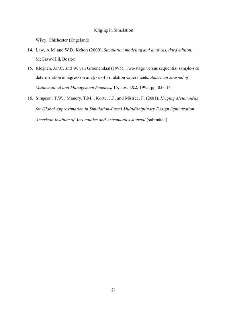
In Kriging, a crucial role is played by the variogram: A diagram of the variance of the

difference between the measurements at two input locations; also see Figure 1, which has


7

(1)

(2)

symbols explained in the next subsection. The assumption of a second-order stationary

covariance process implies that the variogram is a function of the distance (say) h between two

locations. Moreover, the further apart two inputs are, the smaller this dependence is - until the

effect is negligible.

Formal Model for Kriging

A random process Z(@) can be described by {Z(s) : s 0 D } where D is a fixed subset of Rd and

Z(s) is a random function at location s 0 D; see Cressie 6, p. 52.

There are several types of Kriging, but we limit this subsection to Ordinary Kriging,

which makes the following two assumptions (already mentioned above, but not yet formal-

ized):

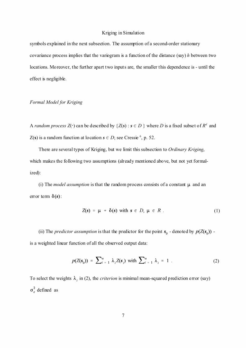
(i) The model assumption is that the random process consists of a constant and an

error term :

(ii) The predictor assumption is that the predictor for the point - denoted by -

is a weighted linear function of all the observed output data:

To select the weights in (2), the criterion is minimal mean-squared prediction error (say)

defined as


8

(3)

(4)

(5)

(6)

To minimize (3) given (2), let m be the Lagrangian multiplier ensuring = 1. Then we

can write the prediction error as

To minimize (4), we utilize the variogram; also see Figure 1. By definition, the variogram is

, where as explained by the stationary

covariance process assumption with and i, j = 1, ..., n. Obviously, we have

= = . The spacing h is also called the lag.

After some tedious manipulations, (4) gives

Differentiating (5) with respect to 81, ..., 8n and m, gives the optimal , ..., :

where denotes the vector , denotes the n×n matrix

whose (i, j)th element is , and denotes a vector of ones; also see Cressie 6 (p. 122).

We emphasize that these opt imal Kriging weights depend on the specific point that

is to be predicted, whereas linear-regression metamodels use fixed estimated parameters (say)

.

The optimal weights (6) give the minimal mean-squared prediction error: (3) becomes


9

(7)

(8)

(9)

(also see Cressie 6 p. 122)

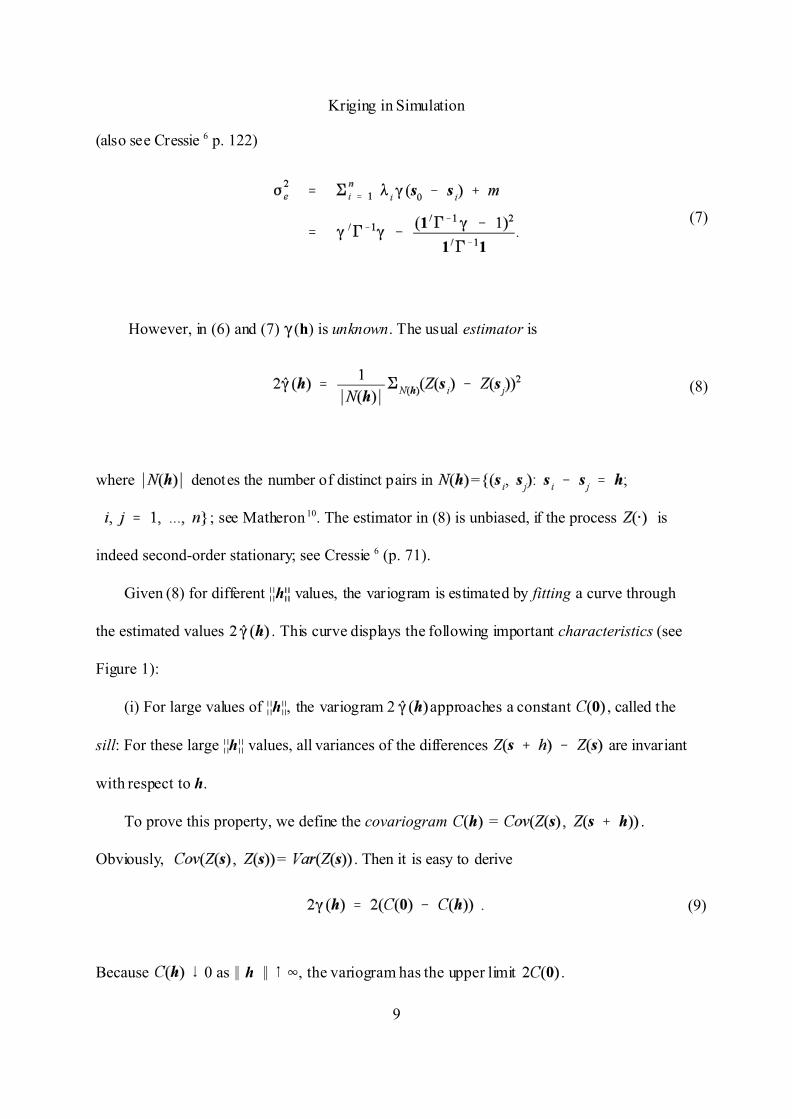
However, in (6) and (7) ((h) is unknown. The usual estimator is

where denotes the number of distinct pairs in =

; see Matheron 10. The estimator in (8) is unbiased, if the process is

indeed second-order stationary; see Cressie 6 (p. 71).

Given (8) for different ||h|| values, the variogram is estimated by fitting a curve through

the estimated values . This curve displays the following important characteristics (see

Figure 1):

(i) For large values of ||h||, the variogram 2 approaches a constant , called the

sill: For these large ||h|| values, all variances of the differences are invariant

with respect to h.

To prove this property, we define the covariogram = .

Obviously, = . Then it is easy to derive

Because 9 0 as 2 h 2 8 4, the variogram has the upper limit .


10

(10)

(11)

(ii) The interval of ||h|| on which the curve does increase (to the sill), is called the range

(say) r ; that is, for . We shall give a specific model in (10).

(iii) Although (9) implies , the fitted curve does not always pass through zero:

It may have a positive intercept - called the nugget variance. This variance estimates noise.

For example, in geostatistics this nugget effects means that when going back to the 'same' spot,

a completely different output (namely, a gold nugget) is observed.

We add that in random simulation, the same input (say, the same traffic rate in queueing

simulation) gives different outputs because different pseudo-random numbers are used. Below

we shall return to this issue.

To fit a variogram curve through the estimates resulting from (8), analysts usually apply

the exponential model

where obviously is the nugget, the sill, and the range. However, other models

are also fitted; for example, the linear model

where again is the nugget; see Cressie 6 (p. 61). Actually, we shall apply (11) in our

experiments, because it is the simplest model and yet gives acceptable results (for example, it

estimates the nugget effect very well).

In deterministic simulation, analysts use more general distance formulas than (8). For


11

(12)

example, Sacks et al.3 (p. 413) and Jones et al.9 (p. 5) use the weighted distance formula

where (with ) measures the importance of the input , and controls the

smoothness of the distance function. To estimate , maximum likelihood estimation (MLE)

is used. The are fixed such that . (We shall briefly return to (12) in our section

Conclusions and Future Research.)

Detrended Kriging

Ordinary Kriging was defined by (1), where was the constant mean of the random

process Z(@). This assumption, however, limits the application of Ordinary Kriging to rather

simple models of the process Z(@). A more general assumption is that is not a constant, but

an unknown linear combination of known functions . This is called

Universal Kriging; see Huijbregts and Matheron 11 (p. 160) and also Cressie 6 (p. 151).

Cressie 6 discusses real (non-simulated) coal-ash data, and Regniere and Sharov 12 discusses

simulated spatial and temporal output data of a random simulation model for ecological

processes.

Now we introduce a novel type of Kriging that we call Detrended Kriging. Detrended

Kriging pre-processes the original data, and then applies Ordinary Kriging to the resulting data

so we can apply software for Ordinary Kriging. For Universal Kriging, however, software is

available only for spatial and temporal data, not for simulation with an arbitrary number of

inputs - to the best of our knowledge.


12

(13)

(14)

We assume that the process mean satisfies the decomposition

where is a known signal function (see, however, the text below (14)) and is a white

noise process that models the measurement error; that is, is normally indentically and

independently distributed with zero mean (NIID). So, we replace (1) by

In practice, the signal function in (14) is unknown. Therefore we estimate

through , from the set of observed (noisy) I/O data . Because

of the assumed white noise, we use ordinary least squares (OLS) to obtain the estimator .

Next we apply Ordinary Kriging to the detrended set .

Our predictor for the output of location is the sum of this Ordinary Kriging prediction and

the estimator .

To test our new Detrended Kriging, we apply classic cross-validation; see Kleijnen and

van Groenendaal 13 (p. 156). Cross-validation eliminates one I/O combination, say ,

from to the original data set , so the remaining data combina-

tions are . This new set gives a prediction

. This process of elimination and prediction is repeated for (say) different combina-

tions ( ). Obviously, if we sort the original set such that the first c observations are

deleted one at a time, then we get k = 1, 2, ..., c.

To summarize the resulting prediction accuracy, we use the norm of the difference

vector (the norm is defined as ). In our experi-


13

(15)

(16)

ments we find that the and norms give simular conclusions.

Note that in Kriging, all prediction errors may be zero at the I/O points that are actually

used to estimate the Kriging model. Therefore we use cross-validation.

Two Examples and Five Metamodels

We are interested in the application of Kriging to discrete-event simulation models, such as

simulated queueing systems. As Law and Kelton 14 - the best selling textbook on simulation -

states (on page 12), a single server queueing system is quite representative of more complex,

dynamic, stochastic simulation models. For further simplification, we suppose that the output

of interest is the mean waiting time in the steady state, E(W). This output can be estimated

through a simulation that uses the following non-linear stochast ic difference equation:

where W(i) denotes the waiting time of customer i, S(i) the service time of customer i, and

A(i) the interarrival time between customers i and i -1. It is standard to start the simulation

run in the empty (idle) state: W(0) = 0. For additional simplification, we assume that the arrival

times form a Poisson process, and so do the service times. This gives the well-known M/M/1

(which can actually be solved analytically; see equation 18 below). By definition, M/M/1

implies that both S(i) and A(i) are identically and independently distributed (IID), so simulation

is straightforward. The output E(W) is usually estimated through the simulation run’s average


14

(17)

(18)

where b denotes the length of the initialization (start-up, transient) phase (which may be zero),

and n the run length. (In M/M/1 analysis and simulat ion through renewal analysis, this

initialization is no issue; in practical simulations, however, it is a major problem; see Law and

Kelton 14 (pp. 496-552).) In other words, the dynamic simulation model generates the time

series (15), but this series is characterized through the single statistic (16).

Actually, simulation is done for sensitivity analysis (possibly followed by optimization).

Such an analysis aims at estimating the input/output (I/O) function (say)

where - following (14) - denotes the (multiple) output and s the (multiple) input . In the

M/M/1 example we have and with arrival rate and service rate .

In general, in (17) has unknown shape and parameters. However, when studying the

performance of a specific simulation methodology, researchers often use the M/M/1 simulation

model because the I/O function is then known - assuming that the methodology has

selected an appropriate initialization length b in (16) (obviously, knowledge of may not

be used by the methodology itself):

Unfortunately, the latter assumption is very questionable: it is well-known that selecting an

appropriate transient-phase length b and run length n in (16) is difficult.

Moreover, Kriging assumes that - in general - the simulation observations have

additive white noise ; see (14). In the M/M/1 example, (14) gives (i) , (ii)

, (iii) normality holds if in (16) uses a sample size (n - b +1) such


15

that an asymptotic central limit theorem holds, (iv) constant variances result if different

simulated traffic rates use different and appropriate sample sizes - see Kleijnen and Van

Groenendaal 15 -and (v) independence results if no common pseudorandom numbers are used.

Altogether, Kriging's (1) or (14) applies to the M/M/1 example only if a slew of assumptions

hold!

Hence, it is much more efficient and effective to generate Kriging test data through

sampling from (13) with instead of (15) and (16). Indeed, our approach

requires less computer time, and guarantees that the white noise assumption holds, including

the desired value for the variance of the white noise. The alternative using (15) and (16) would

require very long runs, especially for high traffic rates this alternative requires .

In conclusion, to test the Kriging methodology we generate data through a static, random

Monte Carlo model like (13) instead of a dynamic stochastic simulation model such as (15)

combined with (16). So, the Monte Carlo technique is both efficient and effective.

Besides Example I, we study Example II representing simulations with multiple local

maxima, which are interesting when optimizing simulation outputs. Example I represents

queueing simulations that show 'explosive' mean waiting times as the traffic rate approaches

the value one. Example II has no specific interpretation.

We sample the white noise-term in (14) through the Matlab function called ‘randn’,

which gives standard NIID variates; that is, has zero mean and unit variance. We also

experiment with a larger variance namely 25; this results in larger error terms, but not in other

conclusions.

To estimate possible values of the L2 norm (defined above), we use 100 macro-replica-

tions. From these macro-replications we estimate L2's median, 0.10 quantile Q0.1, and 0.90


16

quantile Q0.9.

In both examples we take n = 21 equally spaced input values: si with i = 1, ..., 21. For

cross-validation we select (rather arbitrarily) c = 5 inputs values: We eliminate i = 2, 8, 9, 15,

16 respectively. We compared the following five metamodels.

i) Ordinary Kriging

ii) second-degree detrending: is a second-degree polynomial

iii) perfectly specified detrending function: is a hyperbola in Example I, and a fourth

degree polynomial in Example II

iv) fifth-degree detrending: is a fifth-degree polynomial (overfitting)

v) linear regression model that is a second-degree polynomial estimated through OLS.

Note that we also study a perfectly specified detrending function (see iii), because this function

provides a utopian situation: This function gives the mimimum predicion error; in practice,

this function is unknown (otherwise simulation would not be used). Furthermore, it helps us to

verify the correctness of our computer program.

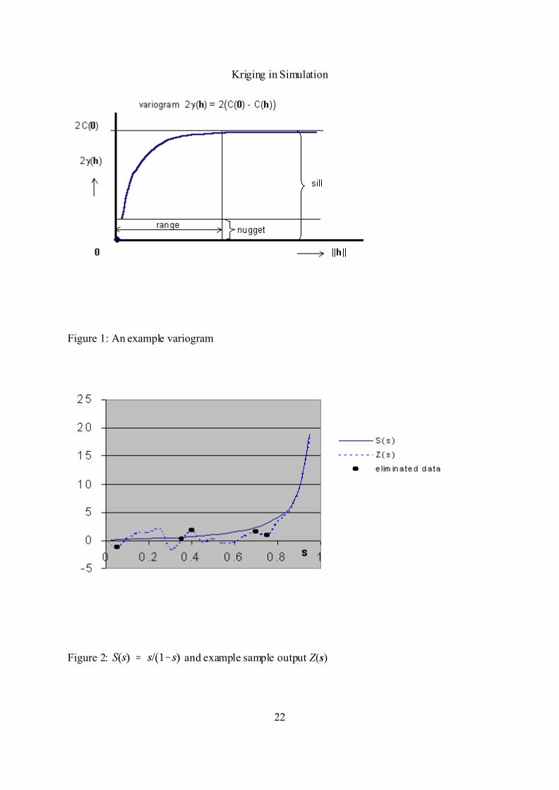
Example I: M/M/1 Hyperbola

We take on , this hyperbolic function may represent

the mean steady-state waiting time for a traffic rate in an M/M/1 queueing system. This

function gives Figure 2, which also displays an example of the noisy output Z(s). The input

locations are . The cross-validation is carried out at s = 0.05,

0.35, 0.40, 0.70, 0.75.

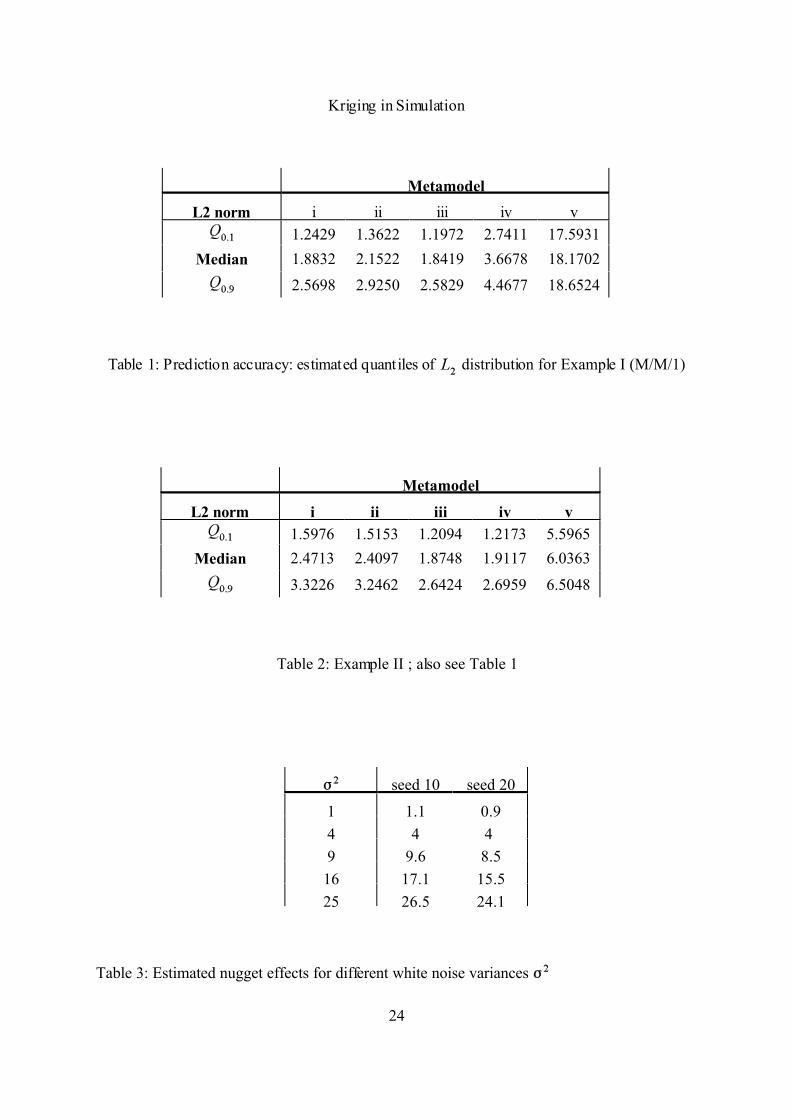
The estimated distribution of the prediction accuracy is summarized in Table 1. This


17

example suggests that metamodel iii (perfectly specified detrending function) gives the best

results. Model i (Ordinary Kriging) is not too bad. Model v (OLS) is simply bad.

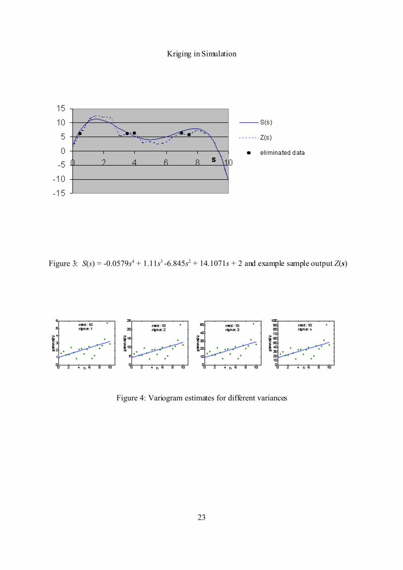
Example II: Fourth-degree Polynomial

We take the following specific polynomial: S(s) = -0.0579s4 + 1.11s3 -6.845s2 + 14.1071s + 2

on . This polynomial has two maxima: A local one and a global one; see

Figure 3. We obtain output for the following 21 input locations . We

cross-validate at .

The estimated distribution of is summarized in Table 2. This example suggests that

metamodel iii (perfectly specified detrending function) gives the best results. Model i (Ordinary

Kriging) is not too bad. Model v (OLS) is simply bad.

Third Example and Nugget Effect

We also wish to better understand the relationship between the nugget effect in (11) and the

variance of the noise in (13). Therefore we perform a simple Monte Carlo experiment:

We take where is NIID with and = 1, 4, 9, 16, and 25

respectively. We sample two macro-replicates, setting the seed of Matlab's ‘randn’ - rather

arbitrary - to the values 10 and 20. In the various Kriging metamodels, we fit the linear

variogram of (11); see Figure 4 (we display results for the seed value of 10 only; note the

different scales for the y-axis in the four plots).

The intercept in (11) estimates the nugget effect; this intercept is presented for different


18

values in Table 3. Obviously, these results confirm our conjecture: The nugget effect is the

variance of the noise.

Conclusions and Future Research

We assume that in practice the mean of the Kriging metamodel (1) is not a constant, but is

a composition of a signal function and white noise. We presented results for two examples of

input/output behaviour of the underlying random simulation model: Ordinary Kriging and

Detrended Kriging gives quite acceptable predictions, whereas traditional linear regression

gives the worst results.

OLS predicts so poorly, because OLS assumes that the fitting errors are white noise,

whereas Kriging allows errors that are correlated; more specifically, the closer the inputs are,

the more positive correlation. Moreover, OLS uses a single estimated function for all input

values, whereas Kriging adapts its predictor as the input changes. Note that OLS may be

attractive when looking for an explanation - not a prediction - of the simulation's I/O behavior;

for example, which inputs are most important; does the simulation show a behavior that the

experts find acceptable (also see Kleijnen1)?

OLS is also compared with (universal) Kriging by Regniere and Sharov 12. Their OLS

model, however, is a rather complicated metamodel (involving terms of order six). The

resulting prediction accuracies are similar for OLS and Kriging.

Further, we found that the nugget effect equals the noise variance.

We restricted our examples to a single input. Therefore we gave each weight in the

more general distance formula (12), the fixed value of one. In design optimization, however,


19

these parameters are used to control the importance of the input variable ; see for example

Simpson et al .16 (p. 8) and Jones et al. 9 (p. 5). In future work we shall investigate multiple

inputs.

Further, we shall relax the assumption of white noise: We shall investigate the effects of

non-constant variances (which occur in queueing simulations), common random number usage

(which creates correlations among the simulation outputs), and non-normality (Kriging uses

maximum likelihood estimators of the weights , which assumes normality). Finally, we shall

apply Kriging to practical queueing and inventory simulations.

Acknowledgment

We thank the two anonymous referees for their most useful comments on an earlier version.

References

1. Kleijnen, J.P.C. (1998), Experimental design for sensitivity analysis, optimization, and

validation of simulation models. In: Handbook of Simulation, edited by J. Banks, Wiley,

New York, pp. 173-223

2. Campolongo, F., J.P.C. Kleijnen, and T. Andres (2000), Screening methods. In: Sensitiv-

ity Analysis, edited by A. Saltelli, K. Chan, and E.M. Scott, Wiley, Chichester (England),

pp. 65-89

3. Sacks, J. , Welch, W.J., Mitchell, T.J. & Wynn, H.P. (1989), Design and analysis of

computer experiments. Statistical Science, 4, no.4, pp. 409-435


20

4. Groenendaal, W.J.H. Van and J.P.C. Kleijnen (1997), On the assessment of economic

risk: factorial design versus Monte Carlo methods. Reliability Engineering and Systems

Safety, 57, pp. 91-102

5. Kleijnen, J.P.C. and J.Helton (1999), Statistical analyses of scatter plots to identify

important factors in large-scale simulations. Reliability Engineering and Systems Safety,

65, no. 2, pp. 147-197

6. Cressie, N.A.C. (1993). Statistics for Spatial Data, Wiley, New York

7. Meckesheimer, M., R.R. Barton, T.W. Simpson, and A.J. Booker (2001), Computational-

ly inexpensive metamodel assessment strategies. American Institute of Aeronautics and

Astronautics Journal (submitted)

8. Koehler, J.R. and A.B. Owen (1996), Computer experiments. In: Handbook of Statistics,

Volume 13, edited by S. Ghosh and C.R.Rao, Elsevier, Amsterdam, pp. 261-308

9. Jones, D.R., M. Schonlau, and W.J. Welch (1998). Efficient global optimization of

expensive black-box functions. Journal of Global Optimization, 13, 455-492

10. Matheron, G. (1962) Traite de Geostatistique Appliquee, Memoires du Bureau de

Recherches Geologiques et Minieres, No. 14, Editions Technip, Paris , (pp.57-59)

11. Huijbregts, C.J. and Matheron, G. (1971). Universal Kriging (An optimal method for

estimating and contouring in trend surface analysis). In Proceedings of Ninth Interna-

tional Symposium on Techniques for Decision-making in the Mineral Industry

12. Régnière, J. and A. Sharov (1999), Simulating temperature-dependent ecological pro-

cesses at the sub-continental scale: male gypsy moth flight phenology. International

Journal of Biometereology, 42, 1999, pp. 146-152

13. Kleijnen, J.P.C. and W. van Groenendaal (1992). Simulation, a Statistical Perspective,


21

Wiley, Chichester (Engeland)

14. Law, A.M. and W.D. Kelton (2000), Simulation modeling and analysis, third edition,

McGraw-Hill, Boston

15. Kleijnen, J.P.C. and W. van Groenendaal (1995), Two-stage versus sequential sample-size

determination in regression analysis of simulation experiments. American Journal of

Mathematical and Management Sciences, 15, nos. 1&2, 1995, pp. 83-114

16. Simpson, T.W. , Mauery, T.M. , Korte, J.J., and Mistree, F. (2001). Kriging Metamodels

for Global Approximation in Simulation-Based Multidisciplinary Design Optimization.

American Institute of Aeronautics and Astronautics Journal (submitted)


22

Figure 1: An example variogram

Figure 2: and example sample output Z(s)


23

Figure 3: S(s) = -0.0579s4 + 1.11s3 -6.845s2 + 14.1071s + 2 and example sample output Z(s)

Figure 4: Variogram estimates for different variances


24

Metamodel

L2 norm i ii iii iv v

1.2429 1.3622 1.1972 2.7411 17.5931

Median 1.8832 2.1522 1.8419 3.6678 18.1702

2.5698 2.9250 2.5829 4.4677 18.6524

Table 1: Prediction accuracy: estimated quantiles of distribution for Example I (M/M/1)

Metamodel

L2 norm i ii iii iv v

1.5976 1.5153 1.2094 1.2173 5.5965

Median 2.4713 2.4097 1.8748 1.9117 6.0363

3.3226 3.2462 2.6424 2.6959 6.5048

Table 2: Example II ; also see Table 1

seed 10 seed 20

1 1.1 0.9

4 4 4

9 9.6 8.5

16 17.1 15.5

25 26.5 24.1

Table 3: Estimated nugget effects for different white noise variances


25

Figure captions and table headings

Figure 1: An example variogram

Figure 2: and example sample output Z(s)

Figure 3: S(s) = -0.0579s4 + 1.11s3 -6.845s2 + 14.1071s + 2 and example sample output Z(s)

Figure 4: Variogram estimates for different variances

Table 1: Prediction accuracy: estimated quantiles of distribution for Example I (M/M/1)

Table 2: Example II ; also see Table 1

Table 3: Estimated nugget effects for different white noise variances

kriging for interpolation in random simulation -...

Documents