No. 2003–33

APPLICATION-DRIVEN SEQUENTIAL DESIGNS FOR SIMULATION EXPERIMENTS:

KRIGING METAMODELING

By Jack P.C. Kleijnen and Wim C.M. van Beers

March 2003

ISSN 0924-7815

SequenDesign16.doc Written: March 21, 2003 Printed: 3/24/2003 11:02 AM

Application-driven Sequential Designs for Simulation Experiments:

Kriging Metamodeling

Jack P.C. Kleijnen 1 and Wim C.M. van Beers 2

1 Department of Information Systems and Management/

Center for Economic Research (CentER)

Tilburg University (UvT), Postbox 90153, 5000 LE Tilburg, The Netherlands

Phone: +31_13_4662029; Fax: +31_13_4663377; E-mail: kleijnen@uvt.nl

http://center.kub.nl/staff/kleijnen/

2 Department of Information Systems and Management

Tilburg University (UvT), Postbox 90153, 5000 LE Tilburg, The Netherlands

Phone: +31_13_4662016; Fax: +31_13_4663377; E-mail: wvbeers@uvt.nl

2

Abstract

This paper proposes a novel method to select an experimental design for interpolation

in simulation. Though the paper focuses on Kriging in deterministic simulation, the

method also applies to other types of metamodels (besides Kriging), and to stochastic

simulation. The paper focuses on simulations that require much computer time, so it is

important to select a design with a small number of observations. The proposed

method is therefore sequential. The novelty of the method is that it accounts for the

specific input/output function of the particular simulation model at hand; i.e., the

method is application-driven or customized. This customization is achieved through

cross-validation and jackknifing. The new method is tested through two academic

applications, which demonstrate that the method indeed gives better results than a

design with a prefixed sample size.

Keywords

Design of Experiments; Simulation; Kriging interpolation; Metamodel; Cross-

validation; Jackknife; Space filling, Latin Hypercube Sampling; Sensitivity analysis

1. Introduction

We are interested in expensive simulations; that is, we assume that a single simulation

run takes ‘much’ computer time (say, its time is measured in days, not minutes).

Therefore we devise a method meant to minimize the number of simulation runs –

that number is called the ‘sample size’ in statistics or the ‘design size’ or ’scheme

size’ in design of experiments (DOE).

We tailor our design to the actual simulation; that is, we do not derive a

generic design such as a classic 2k – p design or a Latin Hypercube Sampling (LHS)

design. We explain the differences between our designs on one hand and classic and

LHS designs on the other hand, as follows.

Classic designs assume a simple ‘metamodel’ (also called approximate model,

emulator, response surface, surrogate, etc.). A metamodel is a model of an

input/output (I/O) function. We denote the metamodel by )(xY where x denotes the k

3

-dimensional vector of the k inputs – called ‘factors’ in classic DOE. In simulation,

the true I/O function is implicitly defined by the simulation model itself (in real-life

experiments, ‘nature’ defines this function). Classic 2k – p designs of resolution III

assume a first-order polynomial function (optimal resolution-III designs are

orthogonal matrices, under various criteria). Central composite designs (CCD) assume

a second-order polynomial function. See, for example, the well-known textbook Box,

Hunter, and Hunter (1978) or the recent textbook, Myers and Montgomery (2002).

LHS - much applied in Kriging – assumes I/O functions more complicated

than classic designs do - but LHS does not specify a specific function for )(xY .

Instead, LHS focuses on the design space formed by the k–dimensional unit cube,

defined by 10 ≤≤ jx (j = 1, …, k) after standardizing (scaling) the inputs. LHS tries

to sample that space according to some prior distribution for the inputs, such as

independent uniform distributions on [0, 1] (or some non-uniform distribution in risk

or uncertainty analysis); see McKay, Beckman, and Conover (1979, 2000), and also

Koehler and Owen (1996) and Kleijnen et al. (2002).

Unlike LHS, we explicitly account for the I/O function; unlike, classic DOE

we use a more realistic I/O function than a low-order polynomial. Therefore we

estimate the true I/O function through cross-validation; i.e., we successively delete

one of the I/O observations already simulated (for cross-validation see Stone 1974; for

an update see Meckesheimer et al. 2002, Mertens 2001). In this way we estimate the

uncertainty of output at input combinations not yet observed. To measure this

uncertainty, we use the jackknifed variance. For jackknifing see the classic article by

Miller (1974); for an update see again Meckesheimer et al. and Mertens.

It turns out that our procedure concentrates on input combinations (design

points, simulation scenarios) in sub-areas that have more interesting I/O behavior. In

our Example I, we spend most of our simulation time on the challenging ‘explosive’

part of a hyperbolic function (which may represent mean steady-state waiting time of

single-server waiting systems). In Example II, we avoid spending much time on the

relatively flat part of the fourth-degree polynomial I/O function with multiple local

hills. (The reader may take a peek at Figures 3 and 6 discussed later.)

We make our procedure sequential for the following two reasons

4

1. Sequential procedures are known to be more ‘efficient’; that is, they require fewer

observations than fixed-sample procedures; see the statistics literature, for example,

Ghosh and Sen (1991) and Park et al. (2002).

2. Simulation experiments proceed sequentially (unless parallel computers are used).

Our Application-Driven Sequential Design (ADSD) does not provide

tabulated designs; instead, we present a procedure for generating a sequential design

for the actual (simulation) experiment.

Note that (after we finished this research, we found that) a different ADSD is

developed by Sasena, Papalambros, and Govaerts (2002). They, however, focus on

optimization instead of sensitivity analysis (we think that optimization is more applied

in engineering sciences than in management sciences, because the latter sciences

involve softer performance criteria). Moreover, they use the ‘generalized expected

improvement function’ assuming a Gaussian distribution, as proposed by Jones,

Schonlau, and Welch (1998). We, however, use distribution-free jackknifing and

cross-validation for a set of candidate input combinations. Sasena et al. examine

several criteria for selecting the next input combination to be simulated, including the

‘maximum variance’ criterion; the latter criterion is the one we use. (An alternative to

their single, globally fitted Kriging metamodel for constrained optimization is a

sequence of locally fitted first-order polynomials; see Angün et al. 2002.) Related to

Sasena et al. (2002) is Watson and Barnes (1995). More research is needed to

compare our method with Sasena et al.’s method (also see our final section, called

‘Conclusions and further research’).

The remainder of this paper is organized as follows. Section 2 summarizes the

basics of Kriging. Section 3 summarizes DOE and Kriging. Section 4 explains our

method, which uses cross-validation and jackknifing to select the next input

combination to be simulated; this section also discusses sequentialization and

stopping. Section 5 demonstrates the procedure through two academic applications,

which shows that our method gives better results than a design with a prefixed sample

size; moreover, estimated Gaussian and linear correlation functions (variograms) –

used in Kriging - give approximately the same results. Section 6 present conclusions

and topics for further research.

5

2. Kriging basics

Kriging is named after a South-African mining engineer, D.G. Krige. It is an

interpolation method that predicts unknown values of a random function or random

process; see Cressie (1993)’s classic Kriging textbook and equation (1) below. More

precisely, a Kriging prediction is a weighted linear combination of all output values

already observed. These weights depend on the distances between the location to be

predicted and the locations already observed. Kriging assumes that the closer the

input data are, the more positively correlated the prediction errors are. This

assumption is modeled through the correlogram or the related variogram, discussed

below.

Nowadays, Kriging is also popular in deterministic simulation (to model the

performance of computer chips, television screens, etc.); see Sacks et al. (1989)’s

pioneering article, and - for an update - see Simpson et al. (2001a). Compared with

linear regression analysis, Kriging has an important advantage in deterministic

simulation: Kriging is an exact interpolator; that is, predicted values at observed input

values are exactly equal to the observed (simulated) output values.

Kriging assumes the following metamodel:

)()()( xxx δµ +=Y with ))(,0(~)( 2 xx σδ NID (1)

6

where µ is the mean of the stochastic process )(⋅Y , and )(xδ is the additive noise,

which is assumed normally independently distributed (NID) with mean zero and

variance )(2 xσ . Ordinary Kriging further assumes a stationary covariance process

for )(xY in (1): the expected values )(xµ are constant and the covariances of

)( hx +Y and )(xY depend only on the distance (or lag) |)()(||| xhxh −+= .

As we mentioned above, the Kriging predictor for the unobserved input 0x -

denoted by )(ˆ0xY - is a weighted linear combination of all the (say) n observed

output data:

Yλxx ⋅=⋅=∑=

/

10 )()(ˆ

i

n

ii YY λ (2)

with ∑ =

n

i i1λ = 1, ),,( 1 ′= mλλ �λ and ),,( 1 ′= myy �Y . To choose these

weights, the ‘best’ linear unbiased estimator (BLUE) is derived: this estimator

minimizes the mean-squared prediction error ( ) ( )( )2000 )(ˆ)()(ˆMSE xxx YYEY −= ,

with respect to λ . Obviously, this solution depends on the covariances, which may be

characterized by the variogram, defined as ))()(()(2 xhxh YYvar −+=γ . (We follow

Cressie, who uses variograms, whereas Sacks et al. use correlation functions; also see

our discussion on the estimation of variograms in Section 5.) An example variogram

is given in Figure 1.

Insert Figure 1

It can be proven that the optimal weights in (2) are

1/

1/

1// 1 −

−

−

−+= Γ1Γ1γΓ11γλ (3)

where γ is the vector of (co)variances /010 ))(,),(( nxxxx −− γγ � ; Γ is the nn ×

matrix whose (i, j)th element is )( ji xx −γ ; /)1,,1( �=1 is the vector of ones. We

point out that the weights in (3) vary with the prediction point, whereas regression

analysis uses the same estimated metamodel for all prediction points. Further details

on Kriging are provided by Cressie (1993, p. 122); an update is Van Beers and

Kleijnen (2003).

7

3. DOE and Kriging

A design is a set of (say) n combinations of the k factor values. These combinations

are usually bounded by ‘box’ constraints: jjj bxa ≤≤ , where Rba jj ∈, with j = 1,

…, k. The set of all feasible combinations is called the experimental region (say) H.

We suppose that H is a k-dimensional unit cube, after rescaling the original

rectangular area (also see the Introduction).

Our goal is to find a design - for Kriging predictions within H - with the

smallest size that satisfies a certain criterion. The literature proposed several criteria:

see Sacks et al. (1989, p. 414). Most of these criteria are based on the Mean Squared

prediction Error, ( ) ( ) 2)()(ˆ)(ˆMSE xxx YYEY −= where the predictor )(ˆ xY follows

from (2) and the true output )(xY was defined in (1). (An alternative considers

)%1(100 α− prediction regions for )(xy and inter-quantile ranges for )(ˆ xy ; see

Cressie 1993, p. 108.) However, most progress has been made through the Integrated

Mean Squared Error (IMSE); see Bates et al. (1996): choose the design that

minimizes

( ) xxx dYIMSEH

)()(ˆMSE φ∫= (4)

for a given weight function )(xφ .

To validate the design, Sacks et al. (1989, p. 416) compare the predictions

with the known true values in a test set of size (say) m. They assume )(xφ to be

uniform, so IMSE in (4) can be estimated by the Empirical Integrated Mean Squared

Error (EIMSE):

( ) .)()(ˆ1 2

1∑

=−=

m

iii yy

mEIMSE xx (5)

Note that criteria such as (4) are more appropriate in sensitivity analysis than

in simulation optimization; see Sasena et al. (2002) and also Kleijnen and Sargent

(2000) and Kleijnen (1998).

4. Application-driven sequential design

4.1 Pilot input combinations

8

We start with a pilot design of size (say) n0. To select n0 specific points, we notice

that Kriging gives very bad predictions in case of extrapolation (i.e., predictions

outside the convex hull of the observations obtained so far). Indeed, in our examples

we find very bad results (not displayed). Therefore, we select the 2k vertices of H as a

subset of the pilot design. In our tow examples with a single input (k = 1), this choice

implies that one input value is the minimum and one is the maximum of the input’s

range; see Figure 2 (other parts of this figure will be explained below, in Sections 4.2

and 4.3).

Insert Figure 2

Besides these 2k vertices, we must select some more input combinations to

estimate the variogram. Like Cressie (1993) we assume either a Gaussian variogram

))exp(1()( 10 ahcch −−+=γ (6)

or a linear variogram

hcch ⋅+= 0)(γ . (7)

Obviously, estimation of these variograms requires at least three different values of h;

thus at least three different I/O combinations. Moreover - as we shall see - our

approach uses cross-validation, which implies that we drop one of the n0 observations

and re-estimate the variogram; i.e., cross-validation necessitates one extra I/O

combination.

In practice, we may select a ‘small’ set of additional observations – besides the

2k corner points – using a standard space-filling design, which ensures that no two

design points are too close to each other. More specifically, we propose a maximin

design, which packs all design points in hyper spheres with maximum radius; see

Koehler and Owen (1996, p. 288). In our examples, we take - besides the two

endpoints of the factor’s range – two additional points. The latter points we place such

that all four observed points are equidistant; see again Figure 2. (Future research may

investigate alternative sizes n0 and components x.)

4.2 Candidate input combinations

9

After selecting and actually simulating a pilot design (Section 4.1), we choose

additional input combinations - accounting for the particular simulation model at

hand. Because we do not know the I/O function of this simulation model, we choose

(say) c candidate points - without actually running any expensive simulations for

these candidates (as we shall see in Section 4.3.

First we must select a value for c. In Figure 2 we select three candidate input

values (had we taken more candidates, then we would have to perform more Kriging

calculations; in general, the latter calculations are small compared with the

‘expensive’ simulation computations).

Next we must select c specific candidates. Again, we use a space-filling design

(as we did for the pilot sample). In Figure 2 we select the three candidates halfway

between the four input values already observed. (Future research may investigate how

to use a space filling design to select candidates, ignoring candidates that are too close

to the points already observed. In practice, LHS designs are attractive since they are

so simple: LHS is part of spreadsheet add-ons such as @Risk.)

4.3 Cross-validation

To select a ‘winning’ candidate for actual (expensive) simulation, we estimate the

variance of the predicted output at each candidate input – without any actual

simulation. Therefore we use cross-validation and jackknifing, as follows.

Given a set of observed I/O data ),( ii yx with ni ,,1 l= (initially, 0nn = ),

we eliminate observation i and obtain the cross-validation sample (with only n – 1

observations):

)},(,),,(),,(,),,(),,{( 11112211)(

nniiiii yxyxyxyxyxS ll −+−−

− = . (8)

From the sample in (8), we could compute the Kriging prediction for the output for

each candidate. However, to avoid extrapolation (see Section 4.1), we do not

eliminate the observations at the vertices: of the cross-validation sample in (8) we use

only (say) nc observations. The predictions are analogous to (2) replacing n by nc; in

case of k = 1 we take nc = n0 – 1. Obviously, we must re-estimate the optimal weights

in (2), using (3) (also see the ‘binning’ discussion at the end of Section 4.4). Figure 2

10

shows the nc = n0 – 1 = 3 Kriging predictions (say) )(ˆ iY − after deleting observation i

as in (8), for each of the c = 3 candidates.

Figure 2 suggests that it is most difficult to predict the output at the candidate

point x = 8.33. To quantify this prediction uncertainty, we use jackknifing.

4.4 Jackknifing

First, we calculate the jackknife’s pseudo-value for candidate j, which is defined as

the following weighted average of the original and the cross-validation predictors:

)()0(

;ˆ)1(ˆ~ i

jcjcij YnYny −− ×−−×= with j = 1, …, c and i = 1, …, nc (9)

where )0(ˆ −jY is the original Kriging prediction for candidate input j based on the

complete set of observations (zero observations eliminated: see the superscript -0).

From the pseudo-values in (9), we estimate the jackknife variance for

candidate j:

2

1;

2 )~~()1(

1~j

n

iij

ccj yy

nns

c

−−

= ∑=

with ∑=

=cn

iij

cj y

ny

1;

~1~ . (10)

Note that we also experimented with other measures of variability, for example, the

90% interquantile; all these measures gave the same type of design.

Finally, to select the winning candidate (say) m for actual simulation, we find

the maximum of the jackknife variances in (10):

})~{arg( 2j

jsmaxm = . (11)

Note that a candidate location close to a deleted observation lies relative far

away from the remaining observations. Hence, such a candidate is less correlated to

its neighboring points. Consequently, its Kriging prediction becomes rather uncertain.

However, this phenomenon holds for each deleted observation.

Note further that to reduce the computer time needed by our procedure (not by

the simulation itself), we estimate the variogram from binned distances: for n inputs,

we classify the n(n – 1)/2 possible distances h in (say) nb < n equally sized intervals

11

or ‘bins’. These intervals should be as small as possible to retain spatial resolution, yet

large enough to stabilize the variogram estimator. Journel and Huijbregts (1978)

recommend at least thirty distinct pairs in each interval. For the nb midpoints of these

intervals, we calculate the average squared difference to estimate the variogram; see

Cressie (1993, p.69). In our examples we use nb = 15.

4.5 Sequentialization

Once we have simulated the ‘winning’ candidate selected through (11), we add the

new observation to the set of observations; see S in (8) – now with superscript (-0)

and with n + 1 members.

Next, we choose a new set of candidates with respect to this augmented set.

For example, in Figure 2 we add as new candidates x = 1.67, x = 5, x = 7.5 and x =

9.17; these candidates are not shown in Figure 2, but the winning candidate is shown

as part of Figure 3.

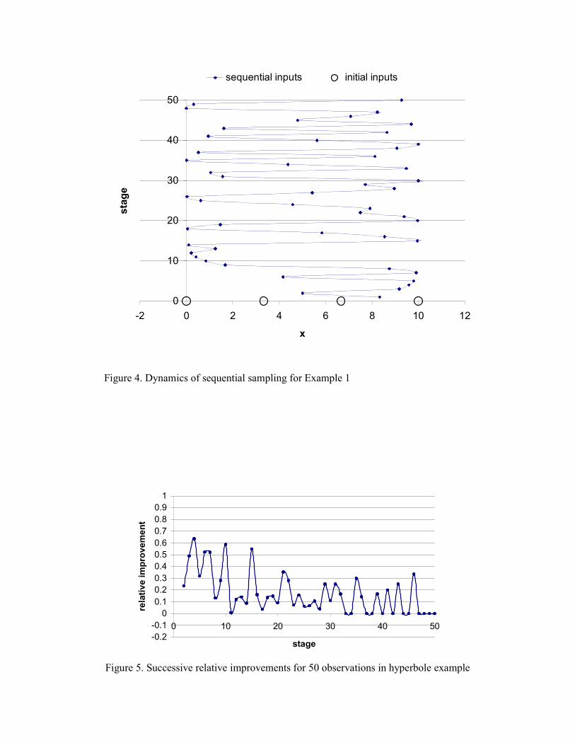
The ‘dynamics’ of our procedure is demonstrated by Figure 4, which shows

the order in which input values are selected - in a total sample size n = 50.

Insert Figures 3a & b

Insert Figure 4

4.6 Stopping rule

To stop our sequential procedure, we measure the Successive Relative Improvement

(SRI) after n observations:

SRIn = 12

122 }~{|}~{}~{| −−− njjnjjnjj

smaxsmaxsmax (12)

where njjsmax }~{ 2 denotes the maximum jackknife variance (see (11)) after n

observations. Figure 5 shows SRI for up to n = 50 in Example I (detailed in Section

5.1). There are no essential changes in (12) beyond n = 15. In the literature (including

12

Sasena et al. 2002 and Jones et al. 1998), we did not find an appealing stopping

criterion for our sequential design; future research may be needed.

Insert Figure 5

We stop our sequential procedure as soon as we find no ‘substantial’ reduction

for SRI. However, SRI may fluctuate greatly in the first stages, so we might stop

prematurely. To avoid such stopping, we select a minimum value (say) nmin so that the

complete design contains min0 nnn += observations. Figure 3(a) used nmin =15,

whereas Figure 3(b) used nmin = 50 (Figure 2 is the part of Figure 3 that corresponds

with n = 4.)

In practice – as Kleijnen et al. (2002) point out –simulation experiments may

stop prematurely (e.g., the computer may break down). Our procedure then still gives

useful information.

5. Two examples

5.1 Example I: a hyperbolic I/O function

Consider the following hyperbole:

xxy−

=1

with 0 < x < 1. (13)

We are interested in this example, because y in (13) equals the expected waiting time

in the steady state of a single-server system with Markovian (Poisson) arrival and

service times (denoted by M/M/1). This system has a single input parameter, namely

the traffic load x, which is the ratio of the arrival rate and the service rate. This system

is a building block in many realistic discrete-event simulation models; see Law and

Kelton (2000, p. 12) and also Van Beers and Kleijnen (2001).

When applying our approach to (13), we decided to select a pilot sample size

n0 = 4 and a minimum sample size value nmin = 10. We stop the sequential procedure

as soon as the SRI in (12) drops below 5%; this results in a total sample size n = 19.

Also see Figure 6(a). Replacing 5% by 1% gives n = 36; see Figure 6(b).

13

Figure 6 demonstrates that our final design selects relative few input values in

the area that generates an approximately linear I/O function, whereas it selects many

input values in the exploding part (where x approaches one).

Insert Figures 6a & b

We think that our design is intuitively appealing - but we also use a test set to

quantify its performance. In this test, we compare our design with a single-stage LHS

design of the same size (n = 19 or n = 36). LHS divides the total range of the input

variable into n mutually exclusive and exhaustive intervals of equal length; within

each interval, LHS samples a uniformly distributed value. To estimate the resulting

variability, we obtain (say) ten LHS samples, from which we estimate the mean and

the standard deviation (standard error).

From the n observations per design we compute the Kriging predictors for the

32 true test values, and calculate the squared error per test value. From the 32 values

we compute the average – see EIMSE in (5), which corresponds with the L2 norm –

and the maximum or ∞L norm. We find substantially better results for our designs;

see Table 1.

insert table 1

5.2. Example II: a fourth-order polynomial I/O function

As Van Beers and Kleijnen (2001) did, we consider

2+14.1071+x6.845-x1.11+x-0.0579y 234 x= , (14)

which is a multi-modal function; see again Figure 2 .

For our design, we select n0 = 4, nmin =10, and a SRI smaller than 5%. This

gives a sequential design with 18 observations. A SRI smaller than 1% gives a final

(sequential) design with 24 observations (Example I resulted in 36 observations).

Figure 7 demonstrates that our final design selects relative few input values in

the area that generates an approximately linear I/O function, whereas it selects many

input values near the edges, where the function changes much.

14

We again compare our design with a single-stage LHS design of the same size

(n = 18 or n = 24), and obtain ten LHS samples to estimate the mean and standard

deviation. We find substantially better results for our designs; see Table 2.

Note that we focus on sensitivity analysis, not optimization. For example, our

method selects input values - not only near the ‘top’ - but also near the ‘bottom’ of

(14). If we were searching for a maximum, we would adapt our procedure such that it

would not collect data near an obvious minimum.

Insert Figure 7

5.3 Estimated variograms: Gaussian versus linear

We also investigate the influence of the assumed variogram, namely a Gaussian

variogram and a linear variogram; see (6) and (7). We use a single-stage design with

21 observations. We use ordinary least squares for these estimators (whereas Sack et

al. assume a Gaussian correlation function and use maximum likelihood estimation,

which takes much more computer time and may involve numerical problems).

The Gaussian and the linear variograms result in two designs that look very

similar, for both Example I and Example II. More precisely, when using a test set of

nine equidistant input values, Kriging predictions based on a Gaussian variogram give

an EIMSE of 0.3702, whereas a linear variogram gives 0.3680 for Example I.

Analogously, Example II gives 0.0497 and 0.0482. So the Gaussian and linear

variograms give similar values for EIMSE. The linear variogram, however, is simpler:

no data transformation is needed.

6. Conclusions and further research

To avoid expensive simulation runs, we propose cross-validation and jackknifing to

estimate the variances of the outputs for candidate input combinations. We actually

simulate only the candidate with the highest estimated variance. This procedure we

apply sequentially.

Our two examples show that our procedure simulates relatively many input

combinations in those sub-areas that have interesting I/O behavior. Our design gives

smaller prediction errors than single-stage designs do.

15

In future research, we may extend our approach to

1. alternative pilot-sample sizes n0 with alternative space-filling input

combinations x (Jones et al. 1998, p. 21 propose n0 = 10k and an adjusted

LHS design)

2. alternative space-filling designs for the selection of candidate input

combinations, ignoring candidates that are too close to the points already

observed in any preceding stages (such an alternative design may be a

nearly-orthogonal LHS design; see Kleijnen et al. 2002)

3. a stopping criterion for our sequential design

4. multiple inputs (k > 1)

5. realistic simulation models (instead of our Examples I and II)

6. comparison of our approach with Sasena et al. (2002)’s approach

7. stochastic simulation models

8. other metamodels, such as linear regression models (see Kleijnen and

Sargent 2000) and neural nets (see Simpson et al. 2001b).

Acknowledgment

Bert Bettonvil (Tilburg University) provided very useful comments on an earlier

version.

References

Angün, E. D. den Hertog, G. Gürkan, and J.P.C. Kleijnen (2002), Response surface

methodology revisited. Proceedings of the 2002 Winter Simulation

Conference, edited by E. Yücesan, C.H. Chen, J.L. Snowdon and J.M.

Charnes, pp. 377-383

Bates, R.A., R.J. Buck, E. Riccomagno and H.P. Wynn (1996), Experimental

design and observation for large systems. Royal Statistical Society. 58, no. 1,

pp. 77-94

Box, G.E.P., W.G. Hunter and J.S. Hunter (1978), Statistics for experimenters: an

introduction to design, data analysis and model building. John Wiley & Sons,

Inc., New York

Cressie, N.A.C. (1993), Statistics for spatial data, Wiley, New York

16

Ghosh, B.K. and P.K. Sen (editors), 1991, Handbook of sequential analysis. Marcel

Dekker, Inc., New York

Jones, D.R., M. Schonlau, W.J. Welch (1998), Efficient global optimization of

expensive black-box functions. Journal of Global Optimization, 13, 455-492

Journel, A.G. and C.J. Huijbregts (1978), Mining geostatistics, Academic Press,

London

Kleijnen, J.P.C. (1998), Experimental design for sensitivity analysis, optimization,

and validation of simulation models. Chapter 6 in: Handbook of simulation,

edited by J. Banks, Wiley, New York, pp. 173-223

Kleijnen, J.P.C., S.M. Sanchez, T.W. Lucas and T.M. Cioppa (2002), A user’s guide

to the brave new world of designing simulation experiments. Working Paper

(preprint: http://center.kub.nl/staff/kleijnen/papers.html)

Kleijnen, J.P.C and R.G. Sargent (2000), A methodology for the fitting and validation

of metamodels in simulation. European Journal of Operational Research, 120,

no. 1, pp. 14-29

Koehler, J.R. and A.B. Owen (1996), Computer experiments. Handbook of statistics,

by S. Ghosh and C.R. Rao, vol. 13, pp. 261-308

Law, A.M. and W.D. Kelton (2000), Simulation modeling and analysis, third

edition, McGraw-Hill, Boston

McKay, M.D., R.J. Beckman and W.J. Conover (1979), A comparison of three

methods for selecting values of input variables in the analysis of output from a

computer code. Technometrics, 21, no. 2, pp. 239-245 (reprinted in 2000:

Technometrics, 42, no. 1, pp. 55-61

Meckesheimer, M., R.R. Barton, T.W. Simpson, and A.J. Booker (2002),

Computationally inexpensive metamodel assessment strategies. AIAA Journal,

40, no. 10, pp. 2053-2060

Mertens, B.J.A (2001), Downdating: interdisciplinary research between statistics and

computing. Statistica Neerlandica, 55, no. 3, pp. 358-366

Miller, R.G. (1974), The jackknife - a review. Biomatrika, 61, pp. 1-15

Myers, R.H. and D.C. Montgomery (2002). Response surface methodology: process

and product optimization using designed experiments; second edition. Wiley,

New York

17

Park, S., J.W. Fowler, G.T. Mackulak, J.B. Keats, and W.M. Carlyle (2002), D-

optimal sequential experiments for generating a simulation-based cycle time-

throughput curve. Operations Research, 50, no. 6, pp. 981-990

Sacks, J., W.J. Welch, T.J. Mitchell and H.P. Wynn (1989), Design and analysis of

computer experiments. Statistical Science, 4, no. 4, pp. 409-435

Sasena, M.J, P. Papalambros, and P. Goovaerts (2002), Exploration of metamodeling

sampling criteria for constrained global optimization. Engineering

Optimization 34, no.3, pp. 263-278

Simpson, T.W., T.M. Mauery, J.J. Korte, and F. Mistree (2001a), Kriging

metamodels for global approximation in simulation-based multidisciplinary

design optimization. AIAA Journal, 39, no. 12, 2001, pp. 2233-2241

Simpson, T.W., J. Peplinski, P.N. Koch, and J.K. Allen (2001b), Metamodels for

computer-based engineering design: survey and recommendation. Engineering

with Computers, 17, no. 2, pp. 129-150

Stone, M. (1974), Cross-validatory choice and assessment of statistical predictions

Journal Royal Statistical Society, Series B, 36, no. 2, pp. 111-147

Van Beers, W.C.M. and J.P.C. Kleijnen (2003), Kriging for interpolation in random

simulation. Journal Operational Research Society (accepted)

Watson, A.G. and R.J. Barnes (1995), Infill sampling criteria to locate extremes.

Mathematical Geology, 27, no. 5, pp. 589-608

|h|

2 var(x)

2 γ(h)

0

variogram 2 γ(h)

Figure 1. An example variogram

-15

-10

-5

0

5

10

15

0 2 4 6 8 10

x

y

Figure 2. Fourth-order polynomial example, including four pilot observations and

three candidate inputs with predictions based on cross-validation, where (-i) denotes

which observation i is dropped in the cross validation.

--- model, O I/O data, × candidate locations, • predictions )(ˆ iY −

(0)

(-2)

(-3)

(-2)

(-2)

(-3)

(-3)

(0)

(0)

-15

-10

-5

0

5

10

15

0 2 4 6 8 10

x

y

sequential design initial data model

Figure 3(a). Figure 2 continued with 19=n observations

-15

-10

-5

0

5

10

15

0 2 4 6 8 10

x

y

sequential design initial data model

Figure 3(b). Figure 2 continued with 54=n observations

0

10

20

30

40

50

-2 0 2 4 6 8 10 12

x

stag

e

sequential inputs initial inputs

Figure 4. Dynamics of sequential sampling for Example 1

-0.2-0.1

00.10.20.30.40.50.60.70.80.9

1

0 10 20 30 40 50

stage

rela

tive

impr

ovem

ent

Figure 5. Successive relative improvements for 50 observations in hyperbole example

0123456789

10

0.0 0.2 0.4 0.6 0.8 1.0

x

y(x)

Figure 6(a). Hyperbole example, including four pilot observations and with 19=n

observations

0123456789

10

0.0 0.2 0.4 0.6 0.8 1.0

x

y(x)

Figure 6(b). Figure 6a continued with 36=n observations

-15

-10

-5

0

5

10

15

0 2 4 6 8 10

x

y

sequential design model initial data

Figure 7. Final design for fourth-order polynomial example with RSI < 1% and n = 24

ADSD LHS

EIMSE ∞L EIMSE (stand. error) ∞L (stand. error)

n = 19 8.90 * 10-4 0.0759 6.14 * 10-3 (4.81 * 10-3) 0.3559 (0.1740)

n = 36 1.19 * 10-4 0.0303 2.76 * 10-4 (9.79 * 10-5) 0.0791 (0.0185)

Table 1. IMSE of two design types for hyperbole (Example I)

ADSD LHS

EIMSE ∞L EIMSE (stand. error) ∞L (stand. error)

n = 18 0.1741 1.0470 0.5855 (0.5574) 3.3011 (1.9706)

n = 24 0.0121 0.2503 0.2473 (0.2112) 2.1212 (1.3837)

Table 2. IMSE for two types of designs for fourth degree polynomial