a feasibility study for an imc application in the mining ... stage at a mine. first, a mathematical...

Univers

ity of

Cap

e Tow

nA FEASIBILITY STUDY FOR

AN IMC APPLICATION IN

THE MINING INDUSTRY

This dissertation has been submitted to the

Department of Electrical and Electronic Engineering

at the University of Cape Town in partial fulfilment

of the requirements for the degree of

Master of Science in Engineering.

by

RJ HACKER

September 1 993

__ ..................... """". ·--··'··- .. " .

The University of Cape Town hns been given . the right to reprnduce this thesis in whole or in part. Copyright is he!<l by the author.

Univers

ity of

Cap

e Tow

n

The copyright of this thesis vests in the author. No quotation from it or information derived from it is to be published without full acknowledgement of the source. The thesis is to be used for private study or non-commercial research purposes only.

Published by the University of Cape Town (UCT) in terms of the non-exclusive license granted to UCT by the author.

Univers

ity of

Cap

e Tow

n

ABSTRACT

This project is a feasibility study using Internal Model Control

strategies to optimise the performance of a secondary and tertiary

crusher stage at a mine.

First, a mathematical model of the plant is_ extracted and

simulated. The viability of using IMC on an unstable process is

considered. Various general objectives are then explained,

whereafter the manually controlled plant is evaluated.

Three strategies are proposed that control the bin levels to .

optimise buffer capacity so that crusher throughput is increased

and efficiency improved. These are tested on a simulator fed

with real plant data to reveal their properties.

Finally, an implementation scheme is then proposed.

- iii -

Univers

ity of

Cap

e Tow

n

ACKNOWLEDGEMENTS

I would like to express my appreciation to Prof. M Braae, my

supervisor, for his continual input and suggestions. Even though

distances hampered communication, his consistent encouragement

made this project both interesting and stimulating.

A big thank-you to my sponsors for providing the funds and

opportunity to make this project a reality.

- ii -

Univers

ity of

Cap

e Tow

n

ACKNOWLEDGEMENTS

ABSTRACT

NOMENCLATURE

1 INTRODUCTION

TABLE OF CONTENTS

ii

iii

ix

1

2 CRUSHER PLANT DESCRIPTION 4 2.1 GENERAL PLANT OVERVIEW . . . . . . . . . . . . . . . . . . . . . . . . . . . . . . . . 4

2.2 DETAILED DESCRIPTION OF CRUSHER STAGES . . . . . . . . . . . . . . . . . . 5

2.3 INTERFACING WITH FEEDRATE CONTROLLER . . . . . . . . . . . . . . . . . . . . 7

2.4 DESCRIPTION OF THE SUPERVISORY CONTROLLER . . . . . . . . . . . . . . . 7

2.5 AVAILABLE SENSORS AND ACTUATORS . . . . . . . . . . . . . . . . . . . . . . . 7

2.6 ERRORS.ASSOCIATED WITH INSTRUMENTATION . . . . . . . . . . . . . . . . 10

2.7 AIMS AND BENEFITS OF AUTOMATIC CONTROL 11

3 CRUSHER PLANT SYSTEM IDENTIFICATION 12 3.1 MODELS OF THE PROCESS COMPONENTS . . . . . . . . . . . . . . . . . . . . . 12

3. 1 .1 MODEL OF THE FEED BIN . . . . . . . . . . . . . . . . . . . . . . . . . . . . . . . . 12

3.1 .1 (a) Using total feed to determine bin integration gain . . . . . . . . 13

3.1. 1 (b) Using level and feed changes to find bin integration gain . . . 1 5

3.1.2 MODEL OF THE FEED BIN SPLITTER . . . . . . . . . . . . . . . . . . . . . . . . . . 17

3.1.3 MODEL OF THE CRUSHER . . . . . . . . . . . . . . . . . . . . . . . . . . . . . . . . 18

3.1.4 MODEL OF THE SCREEN . . . . . . . . . . . . . . . . . . . . . . . . . . . . . . . . . 19

3. 1.4(a) Screen split ratio from totalised weightometer readings . . . . 20

3. 1 .4(b) Screen split ratios from step changes in feed . . . . . . . . . . . 24

3.1.5 MODEL OF THE CONVEYOR BELTS . . . . . . . . . . . . . . . . . . . . . . . . . . 27

3.2 TRANSFER FUNCTION OF THE CRUSHER PLANT . . . . . . . . . . . . . . . . . 28

3.2.1 INPUT VARIABLES . . . . . . . . . . . . . . . . . . . . . . . . . . . . . . . . . . . . 29

3.2.2 OUTPUT VARIABLES . . . . . . . . . . . . . . . . . . . . . . . . . . . . . . . . . . . 30

3.2.3 ASSUMPTIONS OF THE PROCESS . . . . . . . . . . . . . . . . . . . . . . . . . . . 30

3.2.3(a) General assumptions . . . . . . . . . . . . . . . . . . . . . . . . . . . . 30

3.2.3(b) Relationship between screen split ratios and <SecGap> . . 31

3.2.3(c) Relationship between crusher feed and <Sec Gap> . . . . . . 32

3.2.3(d) Relationship between bin level and bin feed . . . . . . . . . . . . 33

- iv -

Univers

ity of

Cap

e Tow

n

3.2.4 PROCESS TRANSFER FUNCTION ............................. 34

3.2.4(a) Feed to the crushers . . . . . . . . . . . . . . . . . . . . . . . . . . . . 34

3.2.4(b) Levels . . . . . . . . . . . . . . . . . . . . . . . . . . . . . . . . . . . . . . 35

3.2.4(c) Product ..... ; . . . . . . . . . . . . . . . . . . . . . . . . . . . . . . . 38

3.2.4(d) Summary of the transfer function . . . . . . . . . . . . . . . . . . . 40

3.3 BLOCK DIAGRAM OF THE CRUSHING PROCESS . . . . . . . . . . . . . . . . . 42

4 IMC CONTROLLERS FOR UNSTABLE PROCESSES 44 4.1 INTERNAL MODEL CONTROLLER DESCRIPTION . . . . . . . . . . . . . . . . . . 45

4.2 STABILITY CONDITIONS FOR IMC . . . . . . . . . . . . . . . . . . . . . . . . . . . 46

4.3 RELATIONSHIP BETWEEN IMC AND CLASSICAL CONTROL LOOPS . . . . 47

4.4 BLOCK DIAGRAM OF THE PROCESS . . . . . . . . . . . . . . . . . . . . . . . . . . 49

4.5 PERFORMANCE OF IMC . . . . . . . . . . . . . . . . . . . . . . . . . . . . . . . . . . 51

4.6 IMC CONTROLLER .................... : . . . . . . . . . . . . . . . . . 54

4.7 IMC FILTER ............................................ 55

4.7.1 EFFECTS OF FILTER 1 . . . . . . . . . . . . . . . . . . . . . . . . . . . . . . . . . . 57

4. 7 .2 EFFECTS OF FILTER 2 . . . . . . . . . . . . . . . . . . . . . . . . . . . . . . . . . . 59

4.8 CONCLUSIONS ............... ·. . . . . . . . . . . . . . . . . . . . . . . . . . 62

5 SIMULATION OF THE CRUSHER PLANT 64 5.1 MENU STRUCTURE OF THE SIMULATOR . . . . . . . . . . . . . . . . . . . . . . 64

5.1.1 MAIN MENU . . . . . . . . . . . . . . . . . . . . . . . . . . . . . . . . . . . . . . . . 64

5.1.2 SETTING THE SIMULATOR PARAMETERS . . . . . . . . . . . . . . . . . . . . . . . 65

5.1.2(a) Input data filename . . . . . . . . . . . . . . . . . . . . . . . . . . . . . 66

5.1.2(b) Output data filename . . . . . . . . . . . . . . . . . . . . . . . . . . . 66

5.1 .2(c) Selecting input feed . . . . . . . . . . . . . . . . . . . . . . . . . . . . 66

5.1.2(d) Graphing information . . . . . . . . . . . . . . . . . . . . . . . . . . . 66

5.1.2(e) Secondary crusher gap . . . . . . . . . . . . . . . . . . . . . . . . . . 67

5.1.2(f) Crusher ON/OFF .. .. .. .. .. .. .. .. . .. . .. .. .. .. .. . 67

5.1.2(g) Fraction of real time . . . . . . . . . . . . . . . . . . . . . . . . . . . . 67

5.1.2(h) Controller Types . . . . . . . . . . . . . . . . . . . . . . . . . . . . . . . 67

5.1.3 RESET THE SIMULATOR . . . . . . . . . . . . . . . . . . . . . . . . . . . . . . . . . 68

5.1.4 SINGLE RUN ................. : . . . . . . . . . . . . . . . . . . . . . . 68

5.1.5 CONTINUOUS RUN . . . . . . . . . . . . . . . . . . . . . . . . . . . . . . . . . . . . 69

5.1.6 MIMIC DIAGRAM . . . . . . . . . . . . . . . . . . . . . . . . . . . . . . . . . . . . . 71

5.2 PROGRAM DESCRIPTION . . . . . . . . . . . . . . . . . . . . . . . . . . . . . . . . . . 71

5.2.1 DESCRIPTION OF THE SIMULATOR MODEL . . . . . . . . . . . . . . . . . . . . . . 72

5.2.2 DESCRIPTION OF THE CONTROLLER ALGORITHM . . . . . . . . . . . . . . . . . . 75

- v -

Univers

ity of

Cap

e Tow

n

5.3 USEFUL LIBRARY ROUTINES . . . . . . . . . . . . . . . . . . . . . . . . . . . . . . . 77

5.3.1 MISCELLANEOUS ROUTINES . . . . . . . . . . . . . . . . . . . . • . . . . . . . . . 77

5.3.2 TEXT WINDOWING ROUTINES . . . . . . . . . . . . . . . . . . . . . . . • . . . . . 78

6 DETAILED OBJECTIVES OF THE CONTROL STRATEGIES 80 6.1 AIMS OF THE CONTROL STRATEGIES . . . . . . . . . . . . . . . . . . . . . . . . 81

6.1.1 PREVENTING BIN DAMAGE . . . . . . . . . . . . • . . . . . . . . . . . . . . • . . . 81

6.1.2 PREVENTING BINS OVERFLOWING . . . . . . . . • . . . . . . . . . . . . . . . . . . 81

6.1.3 MAXIMISING THROUGHPUT AND MINIMISING CRUSHER PASS RATE . . . . . . . 81

6.1.4 MINIMISING OPERATOR INVOLVEMENT . . . . . . • . . . . . . . . • . . . . . • • • 82

6.1.5 BUFFER STORAGE CAPACITY . . . . • . . • . . . . . . . . • . • • . • • . . . • . . . 82

6.1.6 MATERIAL BLENDING • . . • • • • . • . • • • • . . . • . . . . . . . . . . • . . . . . 83

6.2 AIMS OF THE CONTROLLER . . . . . . . . . . . . . . . . . . . . . . . . . . . . . . . 83

6.2.1 MINIMISE CONTROL ACTION . . • . • . . . . . . . • . . . • . . . . . . . . • . . . . 83

6.2.2 Low IMPLEMENTATION COSTS . . . . . . . . . . . • . . • • . • . . . • . . . . . . . 84

6.3 CONCLUSIONS . . . . . . . . . . . . . . . . . . . . . . . . . . . . . . . . . . . . . . . . . 84

7 METHODS USED TO TEST CONTROLLERS AND ANALYZE DAT A 85 7 .1 METHODS USED TO ANALYZE RESULTS . . . . . . . . . . . . . . . . . . . . . . 85

7.1.1 HISTOGRAMS OF THE DATA . . . . . . . . . • . . . . • . . • . • . . . . . . • . . . 85

7.1.2 DERIVATION AND IMPLEMENTATION OF THE MOVING AVERAGE • . . . . . . . . 86

7 .1.3 DERIVATION AND IMPLEMENTATION OF THE MOVING STANDARD DEVIATION . 88

7.1.4 COMPARISON BETWEEN MOVING AND CONVENTIONAL STATISTICS. • . . • • • 89

7.1.5 DERIVATION OF CRUSHER PASS RATE • . . . . . • • . • • • • . . • . . . • . . • . 90

. 7 .1.6 DERIVATION OF TERTIARY CRUSHER RECYCLE RATE • . • . • • • . . . . • • • • • 95

7.2 HEADFEED USED TO EVALUATE THE STRATEGIES . . . . . . . . . . . . . . . 96

7 .3 SAMPLE FEED USED TO TEST CONTROLLERS . . . . . . . . . . . . . . . . . . . . 98

7 .4 CONCLUSIONS . . . . . . . . . . . . . . . . . . . . . . . . . . . . . . . . . . . . . . . . . 99

8 OPEN LOOP ANALYSIS OF THE CRUSHER SECTION 100 8.1 DESCRIPTION OF SUPERVISORY CONTROLLER .................. 100

8.2 STATISTICS OF PLANT UNDER OPERATOR CONTROL ............. 101

8.3 RESULTS OF RUNNING SIMULATOR IN OPEN LOOP ............... 102

8.4 SUMMARY ............................................. 106

- vi -

Univers

ity of

Cap

e Tow

n

9 CONTROL STRATEGIES FOR THE CRUSHER SECTION 108 9.1 TRANSFER FUNCTION OF THE CRUSHER PLANT ................. 109

9.2 STRATEGY 1: CONTINUOUS CONTROL OF SECONDARY AND TERTIARY

CRUSHERS . . . . . . . . . . . . . . . . . . . . . . . . . . . . . . . . . . . . . . . . . . . . 114

9.2.1 OUTLINE OF THE CONTROL STRATEGY ........................ 114

9.2.2 TRANSFER FUNCTION OF THE CRUSHER PLANT ................... 115

9.2.3 DESIGN OF THE CONTROLLER . . . . . . . . . . . . . . . . . . . . . . . . . . . . . 115

9.2.4 PERFORMANCE OF THE CONTROLLER . . . . . . . . . . . . . . . . . . . . . . . . . 117

9.2.5 RESULTS OF THE CONTROL STRATEGY ........................ 120

9.2.6 COMMENTS ON THE CONTROL STRATEGY ...................... 123

9.3 STRATEGY 2: CONTINUOUS CONTROL OF SECONDARY CRUSHERS

AND ON/OFF CONTROL OF TERTIARY CRUSHERS . . . . . . . . . . . . . . . . 1 24

9.3.1 OUTLINE OF THE CONTROL STRATEGY ........................ 124


9.3.3 DESIGN OF THE CONTROLLER . . . . . . . . . . . . . . . . . . . . . . . . . . . . . 125



9.3.6 COMMENTS ON THE CONTROL STRATEGY . . . . . . . . . . . . . . . . . . . . . . 133

9.4 STRATEGY 3: ON/OFF CONTROL OF SECONDARY BINS AND

CONTINUOUS CONTROL OF TERTIARY BINS .................... 134

9 .4. 1 OUTLINE OF THE CONTROL STRATEGY . . . . . . . . . . . . . . . . . . . . . . . . 134


9.4.3 CONTROLLER DESIGN . . . . . . . . . . . . . . . . . . • . . . . . . . . . . . . . . . 135



9.4.6 COMMENTS ON THE CONTROL STRATEGY ...................... 141

9.5 RESOLVING THE DIFFICULTY OF CONTROLLING TWO BINS ......... 141

9.6 CONCLUSION . . . . . . . . . . . . . . . . . . . . . . . . . . . . . . . . . . . . . . . . . . 142

10 COMPARISON OF THE MERITS OF THE CONTROL STRATEGIES 143 10.1 BRIEF OVERVIEW OF AIMS AND CONTROL STRATEGIES .......... 143

10.2 COMPARING CRUSHER PASS RATES VS THROUGHPUT .......... 145

10.3 COMPARING PRODUCT STANDARD DEVIATIONS VS THROUGHPUT . 147

10.4 DETAILED OUTPUT STATISTICS ........................... 148

10.4.1 BIN LEVELS . . . . . . . . . . . . . . . . . . . . . . . . . . . . . . . . . . . . . . . 149

10.4.2 CRUSHER PASS RATE ................................. 151

10.4.3 PRODUCT . . . . . . . . . . . . . . . . . • . . . . . . . . . . . . . . . . . . . . . . 152

10.4.4 SECONDARY CRUSHER GAPS . . . . . . . . . . . . . . . . . . . . . . . . . . . . . 153

10.5 CONCLUDING REMARKS . . . . . . . . . . . . . . . . . . . . . . . . . . . . . . . . . 153

- vii -

Univers

ity of

Cap

e Tow

n

11 CONCLUSIONS

12 RECOMMENDATIONS

BIBLIOGRAPHY

REFERENCES

APPENDIX A: Header file for < misc.c >

APPENDIX B: Header file for < windows.cpp >

APPENDIX C: Mathematical proof

APPENDIX D: Crusher pass rate vs screen split ratios

APPENDIX E: Histograms of results

APPENDIX F: Numerical proof

APPENDIX G: Diskette with simulation software

- viii -

154

158

159

161

162

166

170

172

173

184

185

Univers

ity of

Cap

e Tow

n

ABBREVIATIONS

css FSD

hr

IMC

ISE

min (mins)

mm

ROM

t

tph

SYMBOLS

d(s)

/(s) g(s) (G(s))

k(s)

lm(W)

lpf(s) (LPF(s))

m(s) (M(s)) q(s) (Q(s))

r(s)

s u(s) (u(s))

w

Wl2394

Wl23e2

Wl22e2 y(s) (y(s))

NOMENCLATURE

Secondary crusher Closed Side Setting

Full Scale Deflection

hour

Internal Model Control Integral Squared Error

minute(s)

millimetre

Run Of Mines

metric ton

ton per hour

[rad/hr]

[tph] [tph]

[tph]

process disturbance

IMC filter

SISO (MIMO) plant

Classic SISO controller

Bound of SISO multiplicative uncertainty

SISO (MIMO) low pass filter SISO (MIMO) plant model

SISO (MIMO) IMC controller

Classic input setpoint Laplacian variable

SISO (MIMO) plant input

Performance weight for SISO case

Plant tertiary oversize weightometer Plant tertiary bin feed weightometer

Plant product weightometer SISO (MIMO) plant output

- ix -

Univers

ity of

Cap

e Tow

n

MODEL VARIABLE DEFINITIONS

C On/Off [0, 11 C crusher on/off signal

D On/Off [0, 11 D crusher on/off signal

E On/Off [0, 11 E crusher on/off signal

F On/Off [0, 11 F crusher on/off signal

F3 [tph] Unmodified tertiary crusher feed (i.e. Gate = 1)

Feedc [tph] C crusher feedrate

Feed0 [tph] D crusher feedrate

Feede [tph] E crusher feedrate

FeedF [tph] F crusher feedrate

Gap, SecGap [mm] Generic secondary crusher CSS

Gape [mm] C Crusher CSS

Gap0 [mm] D Crusher CSS

Gate [tit] Generic tertiary bin gate opening

Gatee [t/t] Gate Opening for Bin E

GateF [t/t] Gate Opening for Bin F

Leve le [%] Level of Bin C

Level0 [%] Level of Bin D

Leve le [%] Level of Bin E

Leve IF [%] Level of Bin F

N [times] Crusher pass rate of the ore

Product [tph] Finished crusher product

Sec Feed [tph] Generic feedrate to each secondary crusher

Sec Level [%] Generic secondary level

Sec OS [tph] Secondary oversize of both secondary crushers

Sec US [tph] Secondary undersize of both secondary crushers

TerFeed [tph] Generic feedrate to each tertiary crusher

TerLevel [%] Generic level

TerOS [tph] Tertiary oversize of both tertiary crushers

TerUS [tph] Tertiary undersize of both tertiary crushers

T, [tph] Headfeed tonnage

T2 [tph] Secondary undersize of both secondary crushers

T3 [tph] Secondary oversize of both secondary crushers

T4 [tph] Tertiary undersize of both tertiary crushers

- x -

Univers

ity of

Cap

e Tow

n

GREEK CHARACTERS

G2

G3

E(E)

(

fJ(fJ)

A

CONSTANTS

At.I 0.81

Ag.12 50

K9.12 -800

Ag.tJ -50

Kg.tJ 1300

Ag.a2 -0.053

Kg.a2 1. 7

Ag.aJ -0.025

Kg.aJ 0.98

[t/t]

[t/t]

[rad/hr]

[rad/hr]

[%/t]

[tph/mm]

[tph]

[tph/mm]

[tph]

[(t/t)/mm]

[t/t]

[(t/t)/mm]

[t/t]

SPECIAL NOTATION

Secondary screen split ratio

Tertiary screen split ratio (Nominal) sensitivity function

Damping factor of second order oscillations

(Nominal) complimentary sensitivity function

Tuning parameter for IMC filter

Frequency

Natural frequency of second order oscillations

Bin integration gain

Gain relating SecGap to SecFeed

Constant for above

Gain relating SecGap to TerFeed

Constant for above

Gain relating SecGap to secondary screen split

ratio

Constant for above

Gain relating SecGap to tertiary screen split ratio

Constant for above

[ .. ] All units are enclosed in square brackets e.g. [tph]

< .. > Small signal (AC) value. Note that subscripts are not used here e.g. < GateE > means change in bin E's gate

I· .1 Absolute value ll.. Change in

v For all

- xi -

Univers

ity of

Cap

e Tow

n

1 Introduction

This thesis reports on the results of a feasibility study using various Internal Model

Control strategies to optimise the performance of a secondary and tertiary crusher section

at a mine.

Due to the erratic nature of headfeed in the mining industry, it is usual practice to buffer

the feed to crushers using large storage bins. This enables the crusher feed to be

regulated to suit instantanoous needs without affecting upstream processes. Introducing

bins solves some problems, creates new ones but also presents opportunities of exploiting

its properties.

A bin in the circuit requires constant attention so that it neither empties nor overflows.

An empty bin is damaged by ore that hits the base, and care should be taken not to let a

bin empty under any circumstances. Alarm sensors detect when a bin is full, and

immediately switch off conveyor belts that feed it. This could cause an avalanche of trips

upstream, which is to be avoided.

Other than tending to the instantaneous needs of the crushers, the storage and absorption

capacity of the feed bins is a property that can be used to buffer downstream processes

from upstream irregularities in the medium term. Erratic headfeed can cause temporary

underloads and overloads, decreasing overall efficiency and causing plant stoppages. The

bins could be run at levels that provide maximum plant isolation between upstream and

downstream processes. If headfeed surges are typical causes of the plant being tripped,

the bins should be run at a low level so that surges can be absorbed. Similarly, it would

be wise to run bins fairly full to provide ore to downstream processes during times when

headfeed has stopped. If both cases are equally likely, then the best is to run the bins at

half their capacity.

CHAPTER 1 : Introduction 1

Univers

ity of

Cap

e Tow

n

Sometimes, there are multiple sources of material to downstream processes that are

sensitive to material blend. In this case it is also desirable to have some control of the

blend, and steady source feeds simplify the task.

The process that is under investigation has two crusher sets, one secondary set and one

tertiary set. There are two crusher-bin combinations in each set. After the headfeed has

passed the secondary set, a screen classifies its product from which oversize goes on to

the tertiary bins and undersize continues on its way downstream. Oversize material from

the tertiary set is recycled to the tertiary bin, while undersize joins that of the secondary

set. This is a typical secondary and tertiary crusher assembly.

Presently manual control is used to keep the bins roughly at a desired level. When levels

drop too low, relevant crushers are switched off to let the levels increase, and above an

upper level, they are switched on again. Although experience assists to a large degree,

desired level, too low and upper level depend on individual interpretation, and hence the

potential of using the crusher sets optimally are forfeited. Additionally, controlling the

plant at its optimal point requires continuous attention, which is a rather monotonous and

unstimulating task .. Very soon, a suboptimal operating strategy is chosen that requires

minimal attention.

There are thus potential benefits of applying automatic control in this situation. A

controller will continuously strive to keep bin levels at their various setpoints. Hence

buffer storage is more readily predictable and controllable, and can be changed by

altering the setpoints to suit specific needs. It would also be possible to improve

efficiency by operating the crushers at their optimal conditions and thereby minimising the

pass rate of the ore through the crusher. Apart from these benefits, others are pointed

out in the thesis.

Objectives of this thesis are thus to:

o present a plant model and simulation. Actual plant data is used to extract

component transfer functions. The model is used to build a simulator

which serves as a test platform to evaluate various control strategies, and

real plant data is replayed into the simulator to make results as realistic as

possible.

CHAPTER 1: Introduction 2

Univers

ity of

Cap

e Tow

n

o give detailed aims that each control strategy should strive to satisfy.

Success or failure of a particular strategy depends how well these aims are

met.

o evaluate the plant under manual control using detailed aims as guidelines.

o formulate various control strategies and display results of simulating each

strategy. These strategies are implemented using the Internal Model

Control technique. A manual control simulation is also used as a

reference, so that the comparison between automatic and manual control

has an equivalent basis.

o analyze results derived from the previous objective to enable a sound

comparison to be drawn between all the strategies.

o make proposals of the best strategy based on detailed analysis.

This project is a preliminary feasibility study that is intended to provide justification for

events that eventually lead to a controller being implemented.

CHAPTER 1 : Introduction 3

Univers

ity of

Cap

e Tow

n

2 Crusher Plant Description

This section considers the plant as a whole and describes the subplant which is the topic

of the control study. Overall aims and potential benefits of employing an automatic

controller are also considered.

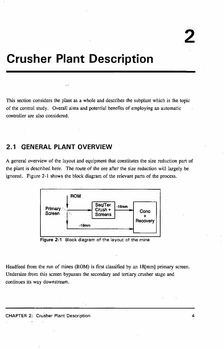
2.1 GENERAL PLANT OVERVIEW

A general overview of the layout and equipment that constitutes the size reduction part of

the plant is described here. The route of the ore after the size reduction will largely be

ignored. Figure 2-1 shows the block diagram of the relevant parts of the process.

I ROM

Primary·. y Screen

-18mm

Sec{fer -18mm Crush+ Screens

- Cone +

Recovery

-

Figure 2-1 Block diagram of the layout of the mine

Headfeed from the run of mines (ROM) is first classified by an 18[mm] primary screen.

Undersize from this screen bypasses the secondary and tertiary crusher stage and

continues its way downstream.

CHAPTER 2: Crusher Plant Description 4

Univers

ity of

Cap

e Tow

n

Oversize is reduced by the secondary and tertiary crusher section until all the ore is

-18[mm], before carrying on downstream.

Of particular interest to this control study is the construction of the secondary and tertiary

crusher stages, which is the topic of the next section.

2.2 DETAILED DESCRIPTION OF CRUSHER STAGES

Primary screen oversize material, with a distribution of + 18-200[mm], is the headfeed to

the secondary and tertiary crusher stages, whose the task it is to reduce the size of the

feed to -18[mm] as efficiently as possible.

The detailed layout is shown in Figure 2-2.

_______ ?...,o..._sl ... s__,.,.. .... w,..,..,,..,,.123"""9..,,..2---------5·-----C 2031s

E F

+18mm

·18mm

TERTIARY BINS AND CRUSHERS

c

__ .......,......_~:)FEED

+18-200mm

D STORAGE BINS

RADIAL GATES

FEED CONVEYORS

)~CRUSHERS

I! I I SCREENS

SECONDARY BINS AND CRUSHERS

Figure 2-2 Secondary and tertiary crusher layout

CHAPTER 2: Crusher Plant Description

20718 c :)

21018 C :) PRODUCT

?~18 -18mm c :) W12292

5

Univers

ity of

Cap

e Tow

n

The ore is fed to the secondary bins from the primary screen via three conveyors: 20118,

20218 and 20318. Only the last conveyor is drawn here. A splitter divides the feed

between secondary bins C and D. There are two large radial gates on the C and D bins

that could be used to control the ore outflow. Two apron feeders, 204 and 205, move the

ore out of the reception bins to the C and D crushers respectively. At the moment, only

the 204 conveyor has a variable speed drive connected to it, although it is assumed that

205 will also have a variable speed drive connected when the crushers are switched to

automatic control. A feedrate controller for the C crusher is currently being planned and

commissioned, and is described later.

The crushed ore is then classified by an 18[mm] screen. Oversize from these screens joins

the oversize from the tertiary screens on conveyor 20618 to be deposited into the tertiary

bins by conveyors 20718 and 20818. The secondary undersize joins the tertiary undersize

on 20918, which is the product conveyor. Conveyors 21018 and 21118 take the product

to the rest of the plant.

As far as the crushers and bins are concerned, the tertiary crusher stage is very similar in

construction to the secondary stage. The only difference is that the tertiary crushers are

choke fed instead of being fed by an apron feeder. However, radial.gates at the bottom

of the tertiary bins could be used to control the amount of ore going into the tertiary

crushers. If this is not feasible, then another method must be found whereby the amount

of ore going to the tertiary crushers may be controlled. One solution is to make the

construction of the tertiary crushers the same as the secondary crushers by introducing

apron feeders, though it involves considerable engineering.

For the control study it is assumed that the ore going to the tertiary crushers is

controllable in some way.

The models for the components are developed in the next chapter; this chapter is confined

to the description of the plant only.


Univers

ity of

Cap

e Tow

n

2.3 INTERFACING WITH FEEDRATE CONTROLLER

A feedrate controller for the C crusher is currently in the process of being commissioned

as part of another project. This controller is designed to maximise feed to the crusher

within the constraints of a variety of overload criteria.

For the purposes of further discussion, it may be assumed that the controller will ensure

that the feedrate to the crusher is kept at its maximum safe operating levels as the crusher

closed side setting (CSS) is manipulated, or ore characteristics change e.g. a decrease in

the CSS will, by means of this minor loop, decrease the feedrate to the crusher to prevent

the crusher being overloaded. As this control loop will merely respond to and higher

level inputs imposed on the crusher, there are no specific interface requirements.

2.4 DESCRIPTION OF THE SUPERVISORY CONTROLLER.

Supervisory controller is used as a general term for a variety of interlocks on the plant

implemented by an overall plant control system, e.g. headfeed is cut should the bin level

exceed a predetermined high alarm limit. Usually, this responsibility rests with the

operator, and for the purposes of this study, it is assumed that these interlocks remain

intact.

Specific details of the supervisory controller are presented in Chapter 8 where the open

loop simulation is discussed. For the moment, it suffices to know that this controller

ensures necessary action is taken if alarm limits are reached.

2.5 AVAILABLE SENSORS AND ACTUATORS

In any process control environment, correct sensing of process variables is of paramount

importance. This is especially true in mining operations where the process variables are

often very difficult to measure. For example, measurements of ore size distributions are

very rarely available. Control objectives therefore h.ave to be realisable in terms of the

available process inputs and outputs.


Univers

ity of

Cap

e Tow

n

On the crusher section concerned, a number of weightometer measurements are available.

Their locations are indicated in Figure 2-2, and are also shown in Table 2(i).

Table 2(i) Weightometers installed on the process

I Sensor No I Description I Wl2292 Tonnage on -18mm product belt 21118

Wl2392 Tonnage to tertiary crusher feed bins on belt 20818

Wl2394 Recycled tertiary crusher product tonnage on belt 20618

Each bin has a level sensor installed. They are summarised in Table 2(ii).

Table 2(ii) Level sensors installed in the feed bins

I Sensor No I Description I Ll221, Level of ore in bin C

Ll22s1 Level of ore in bin D

Ll2311 Level of ore in bin E

Ll2351 Level of ore in bin F

Actuators, or plant inputs as they are known in control, are manipulated by the controller

to yield a desired output or setpoint. Ideally, they would be continuously variable, which

would make them an analogue input. On the other hand digital inputs can have only one

of two values: off and on. Both types of variables are available on the plant, and are

shown in Table 2(iii).

First two on the list are the secondary crushers' CSS. These will affect material drawn

out of the secondary storage bins by means of the feedrate controller. In general,

increasing the CSS causes more material to be removed from the storage bins, and

simultaneously increases the size distribution of the crusher product so that more oversize

material is produced.


Univers

ity of

Cap

e Tow

n

Table 2(iii) Description of available actuators

Actuator Analogue/ Range Description Digital

Gape Analogue 18-30[mmJ CSS of the C and D crushers

Gap0

GateE Radial gate positions at the Analogue 0-1 bottom of feed bins for the E

GateF and F crushers.

C On/Off

D On/Off Digital control line to turn Digital On/Off

E On/Off crushers on and off

F On/Off

Even though the radial gates on the tertiary bins are presently digital, it is quite feasible,

and possible, to convert them to continuously controllable inputs if it is found that a

controller using them is superior to one without. Therefore, for the moment, and at least

for the simulator, it is assumed that there is a continuously manipulable input to change

the feed to the tertiary crushers, and the results of the simulation should indicate whether

or not the plant changes have merit.

Radial gates also appear on the secondary bins, but using them would frustrate the

feedrate controller, which tries to counteract the action taken by the radial gates.

Changing the radial gates on the secondary crushers will actually appear as process

disturbances to the feedrate controller. They are therefore not regarded as available plant

inputs.

The last set of actuators are the digital on/off control of each crusher. Their actions are

obvious: turning the crushers off stops the removal of ore from the bins completely, and

vice versa.


Univers

ity of

Cap

e Tow

n

2.6 ERRORS ASSOCIATED WITH INSTRUMENTATION

Errors associated with instrument readings are important in determining the accuracy of

constants that are derived from the data. This is useful in expressing the confidence of

associated values.

Instrument errors are both systematic and random. Systematic errors, such as zero offset

and gain, can be corrected for if they are known. From time to time, instruments should

be recalibrated to remove any systematic errors.

Random measurement errors are, by definition, not correctable and statistical in nature.

They could arise from uneven belt movement and general instrument noise.

Once the systematic component of measurement errors is removed by calibration, the

random error component is quoted as a percentage of full scale deflection (FSD). Typical

values for weightometers is ±5%, with better weightometers (6 idler type) getting to a

claimed ± 1 % of FSD. Weightometers on the process are all single idler type, so a ± 5 %

error will be used.

Level probe errors can be expressed in a similar way. Random errors arise from the ore

profile in the bins. While filling tip, there will be a peak, and a trough while emptying,

causing the reported level to be incorrect. Careful positioning of instruments could

minimise this error. In addition, multiple echoes to the ultrasonic devices could cause

spurious readings. These all add up to form the level probe errors. A very conservative

error estimate would be ±5 % .

The weightometer and level probe errors are tabulated below. These errors will be used

later to determine the validity of various constants that are derived.

Table 2(iv) Errors of instrumentation

I Tag I FSD I Error I Level Probes 100[%] ±5[%]

Wl22s2 1 OOO[t/hr] ± 50[t/hr]

Wl23s2 1200[t/hr] ± 60[t/hr]

Wl2394 750[t/hr] ± 38[t/hr]


Univers

ity of

Cap

e Tow

n

2.7 AIMS AND BENEFITS OF AUTOMATIC CONTROL

It is generally accepted that judicious application of control can lead to various benefits.

Most notably, efficiencies are almost always improved by relieving the operator of

monotonous, routine tasks such as continuously taking care of the process states. The

operator can use his knowledge more effectively in supervisory tasks, involving automatic

controllers at a lower level.

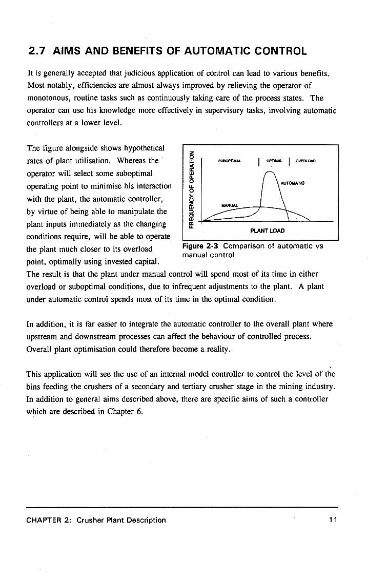
The figure alongside shows hypothetical

rates of plant utilisation. Whereas the

operator will select some suboptimal

operating point to minimise his interaction

with the plant, the automatic controller,

by virtue of being able to manipulate the

plant inputs immediately as the changing

conditions require, will be able to operate

the plant much closer to its overload

point, optimally using invested capital.

SUllOPT1MAL OPTIMAL I OVERLOAD

PLANT LOAD

Figure 2-3 Comparison of automatic vs manual control

The result is that the plant under manual control will spend most of its time in either

overload or suboptimal conditions, due to infrequent adjustments to the plant. A plant

under automatic control spends most of its time in the optimal condition.

In addition, it is far easier to integrate the automatic controller to the overall plant where

upstream and downstream processes can affect the behaviour of controlled process.

Overall plant optimisation could therefore become a reality.

This application will see the use of an internal model controller to control the level of the

bins feeding the crushers of a secondary and tertiary crusher stage in the mining industry.

In addition to general aims described above, there are specific aims of such a controller

which are described in Chapter 6.


Univers

ity of

Cap

e Tow

n

3 Crusher Plant System

Identification

One of the first tasks to complete is the plant modelling exercise, which can be done once

the plant has been analyzed as in Chapter 2. Only thereafter can the controllers be

developed. This chapter will present the plant modelling or system identification.

Models for every subsection of the plant are shown before they are all compiled to form a

block diagram. The block diagram leads to the simulation of the process on a computer

in Chapter 5.

3.1 MODELS OF THE PROCESS COMPONENTS

Models of the components are derived in this section. The models that are considered are

those of the:

• feed bin

• feed bin splitter

• crusher

• screen

. • conveyor belt

3. 1 . 1 MODEL OF THE FEED BIN

It is desired to know the relationship between ore level in the bin to nett incoming

feed. Nett feed is the input less crusher feed.

CHAPTER 3: Crusher Plant System Identification 12

Univers

ity of

Cap

e Tow

n

In fluid dynamics (e.g. a tank containing a liquid), outflow of a bin is level

dependent, whose model is the well known decaying first order exponential.

For the plant under consideration, this assumption cannot be made, since ore

characteristics are certainly not the same as that of a liquid. There are many factors

which determine outflow of material from the bin, least of all bin level. Interparticle

friction effects, not prevalent in liquids, have a much greater influence on material

outflow than bin level. In this application, however, it is assumed that the apron

feeder and radial gates dictate ore outflow from the secondary and tertiary bins

respectively. The secondary CSS _also influences outflow in the case of the tertiary

bins.

Bin level is proportional to the time integral of nett influx of ore. Integration gain

depends on packing density and bin geometry, especially the horizontal cross section.

In mathematical terms, this is expressed as

Leve/(s) = Au(Uo,Yo) [%/tph] (3· 1) Feed(s) s

Two ways of finding Af.1 are described.

3.1.1 (a) Using total feed to determine bin integration gain

If a crusher stops, no ore is removed from the bin and nett feed is simply an

accumulation of bin feed, which is weighed by a weightometer. The ratio of bin

rise to nett feed over the crusher off period gives bin integration gain Af.l.

Since it is essential to know total bin feed and there is no weightometer on the

conveyor belt feeding the secondary bins, the integration gain can only be

determined for the E and F bins. Another problem is that plant data must be

searched for a period during which the tertiary crushers are off that is long

enough so that there is a reasonable increase in bin level ( -20 mins). This

happens quite seldom.


Univers

ity of

Cap

e Tow

n

I ::':fF\EQ!VJ • Avareo;i• J 0 06

j 0 04 0.02

0

I riirv::!1fl 0.02 .

0 0 200 400 600 800 100012001400160018002000 0 200 400 600 800 1000 1200 1400 1600 1800 2000

Timer-I

Figure 3-1 Case 1 for finding bin integration gain

Time laocl

Figure 3-2 Case 2 for finding bin integration gain

Apart from that, if the weightometer is out of calibration and as a result has a

zero offset, the totalised weightometer reading will include the time integral of

the zero offset. The weightometer gain error also increases uncertainty, whereas

. random errors add up to zero. The accuracy of the totalised weightometer

reading is therefore somewhat doubtful, especially due to the zero offset.

The two figures above should indicate another precaution to be taken while

analysing data. \

Both graphs are obtained under the same conditions on the same day (19 June

1992), with the tertiary crushers off during both sample periods. The first graph

in each figure indicates bin level, while the second the corresponding

weightometer reading (both instantaneous and average). Even though average

feed in Case 2 is higher than that of Case 1, bin level rise of Case 1 far exceeds

that of Case 2 (70(%] vs 20[%] rise). Probable reasons are that one bin is full

and incoming material spills over to the second bin, or that the level probe is

saturated and cannot take accurate readings.

During the period 15 June to 25 June 1992, there were nine opportunities to

measure bin integration gain in this way. These samples gave an integration gain

of 0.47 ± 0.07[%/ton].


Univers

ity of

Cap

e Tow

n

3.1.1 (b) Using level and feed changes to find bin integration gain

Another method of finding the integration gain relies on the slope of the level on

a time graph changing as nett feed changes. The change in nett feed could be

due to secondary crushers switching off and thereby causing a step change in

tertiary bin feed. This change in feed is easily measured by the weightometer on

the tertiary bin conveyor belt.

Consider the equation for bin level in the time domain, which involves inverting

(3· l) as shown below, assuming constant feed in the short term:

Level(T) = Af.I* feed* T + C [%]

T is time in [hr], and C is initial value of level in [ % ]

The quantity of interest is slope of the time graph, or Af.l*feed. If the feed

increases by ~feed, then the slope will increase by Af.l*~feed. Ar.1 can be

calculated as the ratio between the changes slope and feed, i.e.

Slope2 - S/ope1 A -ti - Tonnage2 - Tonnage1

[%/~ (3·2)

A striking example of the effect of a feed change can be seen in Figure 3-3.

This is an extreme case, but shows how a step in the feed causes the slope of the

level to decline. The step in feed is 194 - 689 = -495[tph] and the resulting

slope changes by -295 - 248 = -543[%/hr]. Ar.1 is then calculated as

-543/(-495) = 1.10[%/t]. That means that the level will increase by 1.1[%] for

every ton of ore entering the bin.

This calculation is performed several times every day, giving a statistical

distribution of integration gains shown in the histogram of Figure 3-4. A least

squares fit Gaussian curve with a mean of 0. 78 and standard deviation of 0.21 is

drawn to show that the distribution is Gaussian. This histogram contains data of

the period 15 June to 25 June 1992.


Univers

ity of

Cap

e Tow

n

800 989 (t/IVI

700 ...

600 Sloiie • -295 (%/hl1

'C' 500 ,/\ \/ i ~ 400 J Slope•

248 (%/ht

300 '

' 200

FEED 100

0 0.05 0.1 0.15 Time (hr)

Figure 3-3 Finding integration gain

120

100

40

20

0 0

I I

I I

I I

I I

I I

/ I

I

,--

0.2 0.4 0.6 0.8

50

' 45

40

35 ~

30 ~ c

:,..____LEVEL iii 25 :

1'14 [t/hll

0.2

\ \

\ \

\

' ',

1.2

20

15 0.25

.... __ _

1.4 Integration Gain (%/ton)

1.6

Figure 3-4 Histogram of the integration gains obtained for bins E and F together

Values obtained from this statistical analysis are shown in Table 3(i) overleaf,

with means and standard deviations calculated from the original samples using a

spreadsheet, and not the Gaussian curve.


Univers

ity of

Cap

e Tow

n

Table 3(i) Table of average and standard deviation of bin integration gain

Mean [%/t] Std Dev [%/t]

Bin E 0.88 0.21

Bin F 0.75 0.23

Bin E and F 0.81 0.23

The advantage of this technique is that zero offsets have no effect on the resultant

integration gain, since only the change in weightometer reading is required.

Although weightometer gain still influences the calculation, it is an improvement

over the previous method, and is therefore likely to be closer approximation of

the correct integration gain.

Opportunities to apply this technique also arise far more frequently than those for

the previous method, since the secondary crushers often switch on and off due to

a metal detector trip, while the tertiary crushers are almost continuously on. For

example, on 15 June 1992, there was only one opportunity to apply the total feed

method, while there were about 70 for the slope method.

3.1.2 MODEL OF THE FEED BIN SPLITTER

There are always two bins in a set: C and D bins are for the secondary crushers and

E and F bins are for the tertiary crushers. Each set of bins is fed by one conveyor

only, and its material is split evenly between the two bins in the set, except when one

bin is full. Then all the feed spills over .to one bin, and fills up twice as fast as

before, since material inflow doubles.

For simulation purposes, the model of

the feed bin splitter is two gain blocks

with bin feed as the input. The gain Feed~--1

depends on bin level. Take the

secondary crushers for example

0;0.5;1 1-----=-- BinX

1 ;0.5;0 1-----=-- Bin X+1

(X=CandX+l=D). t=igure 3-5 Model of feed bin splitter


Univers

ity of

Cap

e Tow

n

Without either bin full, the gain of both blocks is 0.5. If bin C is full, the gain of

the first block is 0 while that of the second is 1 and vice versa. This is easily

implemented in a program.

Generally, it is not a requirement that the gains of both blocks are 0.5 during normal

operation. They can be any number between 0 and 1, as long as their sum adds to

unity. However, both crushers in a set have the same capacity, which means that for

a fair distribution of workload, gains should be 0.5 in practice.

The significance of this is that the controller must be robust enough so that when one

crusher is taken out of commission, causing its bin to fill eventually, doubling of the

gain should not have a detrimental effect on the control loop.

3.1.3 MODEL OF THE CRUSHER

Many authors have published articles on crusher modelling, with the aim of achieving

a better understanding of the crushing process (Canalog [73], Lynch [77],

Whiten [84]). These models consider the steady state problem, and are very detailed.

A thorough crusher model would split the feed into various size distributions, and

obtain breakage and classification matrices to determine the undersize in crusher

product. However, without information on feed size distributions, ore hardness and

various other parameters, such sophisticated models cannot be applied.

A publication written by Herbst et al [86] considers the problem of controlling

crushers and develops a dynamic model for the crushers using a Kalman filter.

Models that are presented are too complex for this application. They are more of

interest to metallurgists than control engineers. Furthermore, a very involved model

is not necessary for this feasibility study. Also, the feedrate controller described

earlier will hide intricacies of controlling the crusher in any case, further diminishing

the need of an extensive model.

In this application, the secondary CSS can be changed. All other variables are

controlled by the feedrate controller. The relationships of interest are those between


Univers

ity of

Cap

e Tow

n

undersize and feed of both secondary and tertiary crushers, to the secondary CSS.

Without the feedrate controller in place, these relationships cannot be obtained, and

will have to be chosen judiciously.

Time constants that are considered in this application are in the order of tens of

minutes, while crusher dynamics are more in the order of minutes (Herbst et al [86]

and Borrison et al [76]). Therefore, a steady state model of the crusher is sufficient.

A linear relationship between CSS, and the feedrate and undersize fraction is

assumed. This assumption is valid around an operating point, and a controller should

be robust enough to allow deviations from the operating points.

The effect of the CSS on undersize fraction is only felt at the screen stage.

Crusher The influence of CSS on feedrate can be

modelled as shown in the block diagram

alongside. Estimates for .\.rx are given

later in §3.2.3(c).

A I """" ''"'!" ... g.fx, I----:---

< 2 for Secondaries x• 3 for T ertlaries

Figure 3-6 Model of crushers

3. 1 .4 MODEL OF THE SCREEN

At this stage the size reduction of the crusher is realised. The screen separates

crusher product into undersize and oversize material, which has been described in

Chapter 2.

The model of the screen is relatively

simple. Assuming that the screen is

large enough to treat the load, it can

be considered as a device similar to

the feed bin splitter where one block,

which represents the undersize, lets

through a of the feed, and the other,

Underslze

From Crusher

Oversize 1 • « 1----=--

Figure 3-7 Model of the screen

representing the oversize, is 1 - a. The split is dependent on secondary CSS, ore

hardness and crusher feedrate. To simplify the model somewhat, it is assumed that a

is affected only by the CSS in a linear fashion around an operating point. All other


Univers

ity of

Cap

e Tow

n

effects then enter as model uncertainties and disturbances. Relationships between

screen split ratio and secondary CSS could not be obtained, also due to the lack of

data, but using experience to choose these numbers intelligently should not jeopardise

the study.

However, current screen split ratios for the secondary and tertiary screens can be

obtained from weightometer data. Though it does not help in modelling changes in

CSS to screen split ratio, it does give some insight to the way the plant is currently

being operated. Two methods of finding the screen splits are presented: one using

the totalised weightometer readings, and the other using changes in weightometer

readings.

3.1.4(a) Screen split ratio from totalised weightometer readings

Consider the secondary and tertiary crusher construction of Figure 3-8. This is a

flow diagram of the ore. Bins

are ignored, since over a long

period (e.g. a week), total feed is

almost exactly equal to total

product. During the coarse of a

normal week, more than 20000

tonnes of ore can pass through

the crushers. Effects of the

storage bins being able to hold

- 500 tons is insignificant (less

than 2.5%).

Sl!C U/S

: :Wtirdirriii.i£ri!:it : : ·siGJliAL!i ·: ·: ·: ·: ·: ·: · :::i:~~ :K~> .............

Figure 3-8 Block diagram of secondary and tertiary crushers ignoring bins

The weekly totals of the weightometers can then be used to determine secondary

(a2) and tertiary (a3) screen split ratio (the fraction of feed ending in product for

the secondary and tertiary crushers respectively).

In Figure 3-8, the solid triangles represent actual weightometers on the conveyor

belts, while the hollow triangles represent derived values.


Univers

ity of

Cap

e Tow

n

They are found as follows (assuming totalised values)

7; = W/2292 T2 = W/2292 - ( W/2392 - W/23sJ T3 = W/2392 - W/2394 T4 = W/2392 - W/2394

The readings are all in tonnes. From these, a2 and a 3 are determined using

T2 [t/t) «2 = -

7;

0:3 = T4

W/2392 [t/t]

The robustness of these equations is examined at_ the end of this section.

(3·3)

(3·4)

This method of finding a' s is better than looking for a period where all but one

crusher has stopped (in which case weightometer readings would be due to one

crusher only, easily revealing the split ratio), because it seldom happens. The

drawback is that it averages the a's of all crushers, and also changes in ore

characteristics. Other than specifically ensuring that only one crusher operates

for a specific period or that only one type of ore is processed, there is no way of

isolating screen split ratios for a crusher or an ore type, due to the averaging

characteristic.

Data was received for most of March and April 1992, and a program was written

that adds up the weightometer signals on a daily basis. Week's totals can then be

taken and the ratios above calculated. Table 3(ii) shows the results.

The negative result for T2 is unexpected. The equation for T2 involves all the

weightometer signals. Robustness analysis will show that the error of T2 is an

accumulation of the errors of individual weightometers. Therefore, readings for

T2 are very uncertain.

Looking at the layout of the secondary and tertiary crushers (Chapter 2, Figure

2-2), shows that T2 and T3 (secondary undersize and oversize respectively) cannot

be measured directly, but have to be inferred. This leaves only T1 and T4


Univers

ity of

Cap

e Tow

n

Table 3(ii) Weekly totals of weightometer and derived signals

Weightometer

I Derived Totals

I Derived

Totals Values

Week Wl2394 Wln92 Wl2292 I T, I T, I T, I T. I a, a, of 1992 [t) [t) [t) [t] [t) [t) [t)

10 11043 44445 22762 22762 -10640 33402 33042 -0.47 0.75

11 15614 65250 36073 36073 -13563 49636 49636 -0.38 0.76

12 16490 68073 35865 35805 -15718 51583 51583 -0.44 0.76

13 18167 71763 36188 36188 -17408 53596 53596 -0.48 0.75

14 15824 58539 27613 27613 -15303 42916 42916 -0.55 0.73

15 17124 71201 36022 36022 -18055 54077 54077 -0.50 0.76

16 11183 44895 21607 21607 -12105 33712 33712 -0.56 0.75

17 15336 59799 20056 20056 -24406 44462 44462 -1.22 0.74

18 10895 44898 35 35 -33968 34002 34002 -981 0.76

(headfeed and tertiary undersize) at which weightometers can be inserted. T1 is

already measured (by WI2292), leaving only T4 free. Therefore, if greater

accuracy is required in future, it is recommended that a weightometer is used to

measure the tertiary undersize. T 2 would then be calculated using two

weightometers, instead of three, having the accumulated uncertainty of only two

weightometers.

Zero offset of the weightometers once again poses a problem here, as was the

case for the bin integration gain. A zero offset will be included in every reading

taken, and can influence the result significantly, as seen above. Recalibration

would be the easier than inserting another weightometer, and is recommended as

an immediate solution.

The negative value for T 2 causes an incorrect result for a 2, and also casts doubt

as to the validity of a 3, although the value obtained for a 3 ( = 0. 75) seems

plausible.

Robustness of equations (3·3) and (3·4)

This section considers the robustness of the equations used to determine the a's.

Robustness is used loosely here to indicate the error involved in determining a

value by performing mathematical operations using uncertain numbers. If the

error is large, the equation is not very robust.


Univers

ity of

Cap

e Tow

n

Using partial differentiation, the change of a function of two variables can be

expressed as

1a11 = [:;] ax+[:'] ay Xo· Yo Y Xo· Yo

(3·5)

when Llx and Lly are small. The accumulation of the error due to i:nultiple

instruments used to infer a number, is evident. This equation can be used to

determine the uncertainty of equations (3·3) and (3·4).

The errors in weightometer signals are quoted in the previous chapter (§2.6) and

are used to find errors associated with the equations under scrutiny.

Applying (3·5) to (3·3) results in simply adding weightometer errors used in the

calculation. For example, the maximum error for T2 is

la 7;1 s; 1a W/22921 + la W/23921 + la W/2394 1 [tph]

Then, the errors for the derived values are:

Tag Error [mhl % Mean[%]

T1 50 16

T2 148 210

T3 98 39

T4 98 39

The % Mean values are obtained using an average headfeed of 320[tph] and the

screen split ratio information obtained later in §3. l.4(b). It is seen that the error

in T2 is double its expected reading, which is probably the cause of the negative

results in Table 3(ii).


Univers

ity of

Cap

e Tow

n

The errors in the a' s are worked out in a similar way, except this time operating

points for T1' T2 , T3 and Wl2392 are needed.

(3·6)

Using the same numbers as above, these equations evaluate to

l4cx2 1 = 4.8*10-4 14 r; I + 3.1 *10-3 IA T21 = 0.50

14«3 1=s.1*10-4 1aw12392 1+1.s*10-3 1aT4 1=0.10

which shows that the error associated with a2 is half of its range, and therefore

renders any number obtained using this method meaningless. The error of a 3 is

much smaller at 18[%].

The second method of finding the a's is to use step changes in the feed, which is

more accurate.

3.1.4(b) Screen split ratios from step changes in feed

This method of finding a is similar to the one used to determine bin integration

gain. If feed to the crusher changes by ~f (e.g. when the magnetic detector on

the secondary crushers trip), then the product changes by a*~f and oversize by

(1 - a)*~f. If all else remains constant, the step in product can be obtained from

WI2292 and the step in oversize from WI2392• a can determined and traced back to

the origin of the change if needed (any of the four crushers).

aW/2292 (X = [tit] (3·7)

4 W/2392 - A W/2292

There are many instances where this equation can be applied to find the screen

split ratio of the secondary crushers ( a 2), because the feed to the secondary

crushers switches on and off several times a day. It is very seldom that the


Univers

ity of

Cap

e Tow

n

tertiary crushers are switched off, and opportunities to determine a 3 are

correspondingly less.

Advantages of using this technique are similar to that for the integration gain,

and the most important one being that the zero offset of the weightometers have

no effect on the reading.

Figure 3-9 shows a histogram of the values for a 2. that are obtained using the

above method. From this data, a 2 is 0.22 ± 0;03[t/t], with minimum and

maximum values of 0.14 and 0.34 respectively. The Gaussian curve that is

drawn is a least squares fit with mean of 0.21 and standard deviation of 0.042,

and shows that the distribution is roughly Gaussian.

26

~ 20

~ ~ 15

l 10

6

oL-~~~_.__-<2:::....._~~~---'-~---'~===-__J

0 0.05 0.1 0.15 0.2 0.25 0.3 0.35 0.4

«2 Figure 3-9 Histogram of secondary screen split ratio

It could be speculated that the histogram of a2 is in fact a superposition of each

secondary screen split ratio, due to the appearance of what seems like two peaks,

but the evidence is circumstantial. A similar phenomenon appears for the

estimate of a 3 overleaf, but this time it is more pronounced. A Gaussian curve

would be meaningless here due to the wide spread.


Univers

ity of

Cap

e Tow

n

10

8

4

2

O'--~~-'-~~~'---'-~~~~--'---'--~--'

0 ~ ~ u u u ~ u ~ ~

U3

Figure 3-10 Histogram of tertiary screen split ratio

Forty six estimates of a 3 (compared to the 400 for a 2) were obtained during the

same period. These estimates yielded a value of 0.68 ± 0.096 for a 3, with

maximum and minimum values of 0.82 and 0.47. This compares favourably

with the value of 0. 75 obtained using the tqtalised weightometer method in

§3. l.4(a). A histogram of the values for a 3 is shown in Figure 3-10.

These values are summarised in Table 3(iii).

Table 3(iii) Values of screen split ratios using step method

Mean Std Dev Min Max [ton/ton] [ton/ton] [ton/ton] [ton/ton]

02 0.22 0.03 0.14 0.34

03 0.68 0.096 0.47 0.82


Univers

ity of

Cap

e Tow

n

3.1.5 MODEL OF THE CONVEYOR BELTS

The conveyor belt has a relatively simple model of a pure time delay. Two factors

play a role in determining the delay: the speed and length of the conveyor. The gain

of the conveyor is unity.

Mathematically the model is

g(s) = exp-(~~ (3·8)

where: l = length of conveyor in [m]

v = speed of conveyor in [m/hr]

The input and output is tonnage in [tph].

There are eleven conveyors which form part of the secondary and tertiary crushing

system. Table 3(iv) presents a listing the conveyor belt number, length, speed and

dead time.

Table 3(iv) Table of conveyor belt deadtimes

Number Length Speed Deadtime [m] [m/sec] [sec]

20118 46 1.5 31

20218 35 1.5 23

20318 84 1.0 84

20418 5 0.5 10

20518 5 0.5 10

20618 100 1.0 100

20718 5 1.0 5

20818 100 1.0 100

20918 100 1.0 100

21018 5 1.0 5

21118 100 1.0 100


Univers

ity of

Cap

e Tow

n

Even though all these conveyors belong to the secondary and tertiary crusher stages,

only conveyors 20618, 20718 and 20818, which carry the oversize material to the

tertiary bins, are of any importance (see Figure 2-2, Chapter 2). The others either

transport material to the secondary crushers (20118, 20218, 20318), or take it away

(20918, 21018, 21118), and do not influence the control circuit.

Conveyors 20418 and 20518, the apron feeders to crushers C and D respectively, do

not actually have an associated deadtime. The material packing density on the

conveyor does not change as speed changes. Therefore, an increase in the speed of

these conveyors immediately leads to an increase in the material fed to the crushers.

The time delay of conveyors 20618, 20718 and 20818 is about 3.3[mins], which is

insignificant compared to the time scales that are involved here, and therefore it does

not influence the IMC controller performance to any significant extent. Even though

the simulator includes the time delay, it is ignored for the IMC controller design.

Having assembled all the models of the components of the crushing plant, the transfer

function is described next.

3.2 TRANSFER FUNCTION OF THE CRUSHER PLANT

This section describes the development of a transfer function matrix of the plant. The

matrix is a very general one, and will relate all possible inputs and outputs of the plant.

Extraneous elements can be removed at a later stage to meet specific needs of various

control strategies.

This part is divided into four sections:

1. Input Variables: The input variables are described, together with their ranges and

units.

2. Output Variables: The output variables and their ranges are described.

3. Assumptions: Assumptions made for the transfer function and simulator are

highlighted.

4. Relationships between input and output: The relationships tying the inputs and

outputs together using the assumptions and the variables obtained earlier are listed.


Univers

ity of

Cap

e Tow

n

A summary of the relationships is given at the end of this section in the form of a transfer

function matrix. At every stage, tables are provided that list the values of constants.

3.2.1 INPUT VARIABLES

The input variables have been used and described at different stages in various

degrees of detail. This part aims to assemble all these into one input vector.

Plant inputs to the crushers have been analyzed. On the secondary crushers, there

are the CSS of both crushers, and on the tertiary crushers there are the radial gates at

the exit of the tertiary feed bins. Additionally, each crusher can be switched on and

off. The apron feeders on the secondary crushers are already used by the feedrate

controller as described earlier, and therefore are not available as inputs.

There are thus three basic types of inputs available:

1. Secondary crusher gaps: CSS of each secondary crusher is continuously

manipulable. Every crusher has its own setting.

2. Tertiary radial gates: There is a radial gate on each tertiary bin that controls

the feed to the tertiary crushers. These continuously manipulable,

dimensionless inputs have a range between 0 and 1.

3. Crusher On/Off: One input that is available on all the crushers is the digital,

motor On/Off state. There are four such inputs to the system, one for each

crusher. To simplify equations, this will not appear explicitly as an input,

since its function is very simple and straightforward.

In mathematical form, the inputs therefore are

u(s) =

<GapC> <GapD> <GateE> <GateF>

CHAPTER 3: Crusher Plant System Identification

(3·9)

29

Univers

ity of

Cap

e Tow

n

3.2.2 OUTPUT VARIABLES

The outputs are the four bin levels[%] (0% - 100%), four crusher feeds [tph] and

product [tph]:

<Leve/C> <Leve/D> <Leve/E> <Leve/F>

y(s) = <FeedC> <FeedD> <FeedE> <FeedF>

(3· 10)

<Product>

3.2.3 ASSUMPTIONS OF THE PROCESS

Variables for which data was not available have to be chosen with care and

experience. All the assumptions that are made are discussed and motivated.

3.2.3 (a) General assumptions

There is no reason why the two crushers in each set (the two secondary and

tertiary crushers) should have any differences. Both the crushers in a set are

identical and operate under the same conditions i.e. they have the same bin size,

CSS, feed and capacities. Furthermore, secondary and tertiary bin sizes are the

same. It is therefore assumed that constants relating the inputs and outputs of

crushers remain the same in each set. For example, it is assumed that the

relationship between the C crusher CSS and feed to that crusher is no different

from that of the D crusher. Although the size distribution of the material in the

secondary and tertiary bins may be different (affecting packing densities), the

same integration gain will be used for all bins.


Univers

ity of

Cap

e Tow

n

..

3.2.3 (b) Relationship between screen split ratios and < SecGap >

OA

It is assumed that the CSS has a linear relationship with a 2 and a 3, i.e.

a is dimensionless, or could be [t/t]. Note that the average value of the

secondary gaps is used for determining a 3•

The relationship between < SecGap > , and a 3 and a 3 has to be estimated.

Reasonable numbers, would be:

I Ag.a

I Kg.a

I [mm-1]

a2

I -0.053

I 1.7

I 0!3 -0.025 0.98

Effects of these constants on a 2 and a 3 can be seen in Figure 3-11 and

Figure 3-12 below.

(3·11)

An 18[mm] secondary CSS gives an 85 % undersize rate for the secondary

product and a 58 % for the tertiary product. Similarly, at a secondary gap of

24[ mm], the secondary undersize drops to 42 % and tertiary to 38 % . Estimates

for the tertiaries are quite conservative.

U!~---------~

OA

• o.e ., OA •

O'--~~~~~~~-~....__,

W tt ~ ~ ~ Z ~ M a a ~

- ... 1 ...... 1

Figure 3-11 Graph of a2 vs SecGap

O'--~~~~~~~~~--'

W tt ~ ~ ~ Z ~ M M a ~ s.caap[ ...... J

Figure 3-12 Graph of a3 vs SecGap


Univers

ity of

Cap

e Tow

n

As soon as real data becomes available from future results in another project,

these numbers can be changed readily to improve the model.

3.2.3 (c) Relationship between crusher feed and < SecGap >

Crusher feed is also assumed have a linear relationship to secondary gaps. The

secondary feed changes by way of the feedrate controller, while tertiary feed due

to particle size change in the tertiary circuit.

[tph] SecFeed = A9.t2 SecGap + K9.,2

(3·12) TerFeed = (A9.13 SecGap + K9.,a) Gate = F3 Gate [tph]

where

[tph) (3·13)

is the feed to each tertiary crusher when the gates are fully open.

This is the equation for the feed to each crusher separately. Note again that the

average value of the secondary gaps is used to get tertiary crusher feed. The

gate, which has a value between 0 and 1, also regulates feed to the tertiary

crushers.

It makes sense to assume that feed to the secondary crushers would increase as

CSS increase, but the generally larger oversize feed to the tertiary crushers

would cause feed to the tertiary crushers to decrease. The following constants

are suggested.

A,,.f Kg.f [tph/mm] [tph]

SecFeed [tph] 50 -800

TerFeed [tph] -50 1300


Univers

ity of

Cap

e Tow

n

100.--~~~~~~~~~~ -!IOO -Loo

I: 0

-100 .

700 -500

i-

i: 100

0

-100

-300'--~~~~~~~~~--..i ·ZOO'--~~~~~~~~~..___,

10 12 14 1e 1a ao zz 24 a 2111 30 8eoaap(lllmJ

Figure 3-13 Graph of secondary crusher feed vs SecGap

ro ~ M ~ ~ ao zz 24 2111 2111 30 -...1-1

Figure 3-14 Graph of tertiary crusher feed vs SecGap (Gate = 1)

The graphs of the effect on feed· are shown above.

At a secondary CSS of 18[mm], the feed to each secondary and tertiary crusher

is lOO[t/hr] and 400[t/hr] respectively. An increase in CSS to 22[mm] causes the

feed to each secondary crusher to increase to 400[t/hr], and each tertiary crusher

to drop to 200[t/hr] due to the larger sized material.

3.2.3 (d) Relationship between bin level and bin feed

It is assumed that the bin is a pure integrator of nett feed, and that bin outflow is

independent of the bin level. While accurate data is not available, it is assumed

that all bins have the same integration gain. The relationship between the level

and nett feed has been established to be

A level(s) = _!:!. Feed(s) [%]

s (3·14)

Ar.1 is known for the tertiary bins, and the secondary bins have the same gain, in

accordance with the above discussion.

Ar.1 [%/t] 0.81


Univers

ity of

Cap

e Tow

n

Now that all the assumptions and constants have been stated, the transfer function

of the process can be developed.

3.2.4 PROCESS TRANSFER FUNCTION

The binary interaction matrix is a precursor to the transfer function matrix. It is very

useful, since relationships between inputs and outputs can be seen at a glance.

Setting up the BIM gives


x 0 0 0 <leve/C>

0 x 0 0 <Leve/D>

x x x x <Leve/E>

x x x x <Leve/F>

x 0 0 0 <FeedC>

0 x 0 0 <FeedD>

x x x 0 <FeedE>

x x 0 x <FeedF>

x x x x <Product>

The level of the C and D bins are affected by one input each, the corresponding

crusher gap. Levels of the E and F bins are affected by all inputs. Similarly, the

rest can be read off. This BIM is also useful in determining whether the IMC

controller is to be multivariable or not.

Individual transfer functions can now be found using all the information presented.

3.2.4 (a) Feed to the crushers

Crusher feedrate is considered first, because these equatfons will be used in

determining bin levels later. The feed to the secondary and tertiary crushers

have already been discussed in §3.2.3(c), equation (3· 12). However, in control,

the change in a variable rather than the absolute value is relevant. The DC terms


Univers

ity of

Cap

e Tow

n

are usually removed by integral action. Partial differentiation is used for this

purpose, and leads to

<FeedC> = A0.12<GapC>

<FeedD> = A0.12<GapD>

<FeedE> = A Gate <GapC> + <GapD> g.f3 E 2

i= ""'F> _ A G ., <GapC> + <GapD> < r88u1 - g.fS 81'6 F ,

2

+ F3 <GateE> (3·15)

+ F3 <GateF>

The last two equations require the operating point in order to be evaluated. The

numbers for the. constants are given in §3.2.3.

3.2.4 (b) Levels

The first four outputs of the process transfer function concern the four bin levels.

Transfer functions of the C and D levels are fairly straightforward, which,

looking at the BIM, are to be controlled by the secondary CSS. Since the

incoming feed to the bins (i.e. the headfeed) is not known, it is considered to be

disturbance that is either a constant, or a step function. The nett influx of

material is incoming less crusher feed, but, since the incoming feed is considered

to be a disturbance, the nett feed to be integrated is the outflow only (i.e. the

crusher feed), equation (3· 15).

Integrating the nett feed, and using small signal values, gives:

<Leve/C> = -A A

f.t g.f2 <GapC> s

-.4 A ,_.,,, 11•12 <GapD>

s

(3·16)

<Leve/D> =

It is negative because an increase in the gap causes a decrease in the level.


Univers

ity of

Cap

e Tow

n

Inserting the constants gives:

<Leve/C> = -0·81 *50 <GapC> = -41 <GapC> [%] s s

<Leve/D> = -41 <GapD> [%] s

The transfer functions of < LevelE > and < LevelF > are a little more involved

than those of < LevelC > and < LevelD > , because the feed to the tertiary bins

comes from both secondary and tertiary crushers together.

Consider bin E. Feed to bin E is half of the material on the tertiary bin

conveyor belt which carries oversize from the secondaries and terti(U'ies together.

First consider secondary crusher oversize.

Secondary crusher feed is given by (3· 12), of which (1 - a 2) becomes oversize,

where a 2 is given by (3· 11). This gives

SecOS = (1 - a.a)Feed0 + (1 - a.a)Feed0

Inserting (3· 11) and (3· 12), and applying partial differentiation, gives

<SecOS> = [-A9.v.2Feed0 + (1 - uJA9.12]<GapC>

+ [-A9.v.2Feed0 + (1 - ua)A9.12]<GapD>

Now consider the tertiaries:

F3 is defined as the feed to the tertiary crushers when the gates are fully open

and therefore, tertiary crusher feed becomes

FeedE = F3 GateE

FeedF = F3 GateF (3·17)

Then

TerOS = (1 - a.a)F3 GateE + (1 - ua)f=a GateF


Univers

ity of

Cap

e Tow

n

and applying differentiation again gives

<TerOS> = [(-Y2Ag.113)F3 GateE + (1 - cxs)(Y2Ag.ts) GateE)<GapC> +

[(-1f2Ag.11s)F3 GateE + (1 - cxs)(112Ag.ts) GateE)<GapD> +

[(1 - us)F3 ]<GateE> +

[(-1f2Ag.113)F3 GateF + (1 - cxs)(112Ag.f3) GateF]<GapC> +

[(-1f2Ag.113)F3 GateF + (1 - cxs)(V2Ag.ts) GateF)<GapD> +

[(1 - cx 3)F3 ]<GateF>

remembering that the average of the secondary gaps is used to determine a 3•

The feed to the crusher is

<FeedE> = ((%Ag.ts> GateE]<GapC> +

[(112Ag.ra> GateE]<GapD> +

F3 <GateE>

Nett feed to bin E is half of the oversize from the secondary and tertiary

crushers, less the feed to crusher E. This gives

A <Leve/E> = ~ [ V2{<SecOS> + <TerOS>) - <FeedE>)

s

To summarise then, the equation for bin E is

· A . (3·18) <Leve/E> = ;' (g3.1<GapC> + g3.2<GapD> + g3.3<GateE> + g3.4<GateF>)

with

- cx~Ag.12) - cxs)(112Ag.13) GateE)

- cxs)(V2Ag.13) GateF)

(-Ag.112 Feed0 + (1 - cx~Ag.12) g3.2 = ~ + (-V2Ag.11a Fa GateE + (1 - cxs)(V2Ag.1a) GateE) - (V2Ag.1a) GateE

+ (-112Ag.aaFa GateF + (1 - cxs)(V2Ag.1a) GateF)

U3.3 = 112[(1 - cxs) Fa] - F3

Ua.4 = 112[(1 - cxs) Fa]


Univers

ity of

Cap

e Tow

n

For bin F, the equation is

A (3·19) <Leve/F> = ;' (g4.1<GapC> + g4.2<GapD> + g4.3<GateE> + g4.4<GateF>)

with

1 = - + 2

(-A9.u2 Feedc + (1

(-1/2Ag.at3 F3 GateE + (1

+ (-112Ag.at3F3 GateF + (1

- cx~Ag.t2) - cx3)(1/2A9.,3) GateE)

- cxa)(1/2A9.,3) GateF)

(-A9

.u2 Feed0 + (1 - ex~ A9,,2)

g4.2 = ~ + (-112Ag.at3 F3 GateE + (1 - cxa)(1/2Ag.f3) GateE) - (112Ag.f3> GateF + (-112A9.u3F3 GateF + (1 - cxa)(1/2A9.t3) GateF)

g4.3 = 112[(1 - CX3) F:J

g4.4 = 112[(1 - cxa) F3] - F3

The above equations all rely heavily on an operating point, and they all collapse

into one number once it is established.

3.2.4 (c} Product

The last output is crusher product, which is the sum of secondary and terttary

undersize. The undersize can be found in a way similar to the oversize of the

crushers when the level equations were considered.

The secondary undersize therefore is

<SecUS> = [A9.«2 Feedc + cx2 Ag.,2]<GapC>

+ [A9.«2 Feed0 + cx2 A9.,2]<GapD>


Univers

ity of

Cap

e Tow

n

and the tertiary undersize is

< TerUS> = [(V2A0.a3) F3 GateE + a 3(Y2A0.13) GateE]<GapC> +

[(V2Ag.a3) F3 GateE + a 3(Y2A0. 13) GateE]<GapD> +

[a3 F3 ]<GateE> +

[(V2Ag.a3 ) F3 GateF + a3(V2A0.13) GateF]<GapC> +

[(1/2Ag.a3 ) F3 GateF + cx3(V2A0.13) GateF]<GapD> +

[cx3 F3]<GateF>

To summarize, the product is

<Product> = g9.1<GapC> + 992<GapD> + g9.3<GateE> + 99.4<GateF> (3·20)

with

A0.a2 Feed0 + cx 2Ag.12

99.1 = + 1/2A0.a3 F3 GateE + cx3 112A0.13 GateE

+ 112A0.a3 F3 GateF + cx3 112A0.13 GateF

A0.a2 Feed0 + cx2Ag.12

99.2 = + 112A0.a3 F3 GateE + cx3 112A0.13 GateE

+ 1/2A0.a3 F3 GateF + cx3 112Ag.13 GateF

"9.3 = CX3 F3

99.4 = CX3 F3


Univers

ity of

Cap

e Tow

n

3.2.4 (d) Summary of the transfer function

The transfer function of the secondary and tertiary crushers have been presented

in detail above. This section serves as a summary.

With the inputs and outputs defined as

<leve/C> <leve/D>

<GapC>- <Leve/£> <leve/F>

u(s) = <GapD> y(s) = <FeedC> <GateE> <GateF> <FeedD>

<FeedE> <FeedF>

<Product>

the transfer function of the process is


-At.1A2.12 0 0 0 <Leve/C> s

0 -A,,,A2.12 0 0 <Leve/D> s

A A,,, A,,, A,,, f.I {} $93.2 $93.3 -;9u <Leve/E> s 3.1

G(s) = A A,,, A,,, 9. A,,, (3·21) _!:!_ 9.

$94.2 $94.4 <Leve/F> s 4.1 s 4.3

Ao.12 0 0 0 <FeedC>

0 Ag.12 0 0 <FeedD>

Y2Ag.13 GateE 1/zAg.13 GateE FeedE 0 <FeedE>

1/zAo-13 GateF Y2Ag.13 GateF 0 FeedF <FeedF>

99.1 9e.2 9u 99.4 <Product>


Univers

ity of

Cap

e Tow

n

The constants for equation (3·21) are:

(-A0.u2 Feedc + (1 - «JA0.12 ) 1 93.1 = ~ + (-1/2A0.u3 F3 GateE + (1 - «J(1/2A0.13) GateE) - (112A

0.13) GateE

+ (-112Ao.113F3 GateF + (1 - «J(1/2A0.13) GateF)

(-A0.112 Feed0 + (1 - «JA0.12)

g3.2 = ~ + (-112A0 . ..a Fa GateE + (1 - «J(V2A0.13) GateE) - (1/2A0

.13) GateE + (-112Ag.u3F3 GateF + (1 - «J(1hA0.13 ) GateF)

93.3 = 112((1 - «:J F3] - F3

g3.4 = 112((1 - «J F3]

(-A0.112 Feedc + (1 - «J A0.12 )

g4.1 = ! + (-112A0 ... 3 F3 GateE + (1 - iia)(112A0.13) GateE) - (1/2A0

.13) GateF

+ (-112Ag.u3F3 GateF + (1 - cxa)(1/2A0.13) GateF)

(-Ag.u2 Feed0 + (1 - «JA0.12)

94.2 = ~ + (-112A0.u3 F3 GateE + (1 - «J(112A0.13) Gat~E) - (112A0

.13) GateF

+ (-1l2Ao.113F3 GateF + (1 - cx:J(112A0.13) GateF)

g4.3 = 112((1 - cx:J Fa)

94.4 = 112[(1 - cx:J F3] - F3

A0.u2 Feed0 + «2Ag.12

99.1 + %A0.sa F3 GateE + cx31/2A0.13 GateE

+ 112A0 ... 3 F3 GateF + cx3 112A0.13 GateF

Ag ... 2 Feedo +. «2Ag.r2

g9.2 = + 1/2A0.&3 Fa GateE + cx31/2A0.13 GateE

+ 1hA0 . ..a Fa GateF + cx3 112A0.13 GateF

99.3 = «3 Fs

9e.4 = «s Fs


Univers

ity of

Cap

e Tow

n

3.3 BLOCK DIAGRAM OF THE CRUSHING PROCESS

Having studied individual components of

the crushing process in detail, they can be F

assembled into a block diagram as shown

in Figure 3-15.

This block diagram was drawn with the

aim of being able to simulate it on a PC,

hence the node numbering.

7

The headfeed enters at F (1). It then goes

to k1, the secondary bin feed splitter, and

its operation is explained in §3.1.2.

During normal operation, k1 = 0.5,

meaning that half the headfeed goes to bin

C along 2, and the other half to bin D

along 8. The feed to the crusher at G 1

(5), is subtracted from 2 to give the nett

feed to bin C at 3. This is integrated and

the level of bin C appears at 4. Figure 3-15 Block diagram of the crushing process

There is some logic involved around nodes 2,3,4,5, so that no material can be sent to

crusher C unless bin C is not empty (node 4 > 0). Node 4 can also not go above

100[%] or below 0[%].

Material at 5 then goes to the C screen whose split ratio a 2 depends on secondary CSS.

Undersize material becomes product along 6,31,32. The difference between 5 and 6 is

oversize, which is fed to the tertiary conveyor belt along 7,14,15.

The same process is repeated for all crushers.

The conveyor belt carrying oversize material to the tertiary bins is between 15 and 16,

and has a time delay of 0.057[hr], or 205[sec]. Material at 16 is once again split up

evenly between bins E and F during normal operation. Recycled (oversize) material goes


Univers

ity of

Cap

e Tow

n

from 22,28 along 29,15 to the tertiary conveyor. Product is routed from 21,27 via 30 to

prpduct node 32.

This block diagram is suited for the simulator, presented in Chapter 5.


---·--------------------

Univers

ity of

Cap

e Tow

n

model. The controller q(s) would not even know whether input or output saturation has

occurred (although it would be beneficial if it does), and therefore the well known

integral windup is avoided. Continuing with the same idea, the model does not have to

reside in the control law, but can even be a pilot plant running in parallel to a big

industrial process.

4.2 STABILITY CONDITIONS FOR IMC

To assess the conditions for internal

stability, all possible input to output

transfer functions are required. For this

purpose, the block diagram of Figure 4-2

is used. Independent outputs are u, y and

y', while inputs are r, ul and u2.

r +

+ +

u1

y

u2

y' -

The relationship between all inputs and

outputs are obtained by block diagram

algebra ..

Figure 4-2 Block diagram for assessing stability

Assuming the model is exact, the following matrix of equations is obtained:

(1 - gq)g g2q l ( r l -g2q (1 + gq)g u1 (4·1)

-gq gq u2

The condition for internal stability of any process (including non-linear) is that the outputs

must be bounded for bounded inputs, i.e. there exists a number e > 0 such that

IYI < e 'V lul<~. ~>O

The requirement that the poles of a linear system must be on the closed left half of the

s-plane (the origin excluded) for stability is a direct consequence of this definition.

CHAPTER 4: IMC Controllers for Unstable Systems 46

Univers

ity of

Cap

e Tow

n

By inspection, the outputs of (4· 1) are bounded for all bounded inputs if g and q are

stable, in which case the internal stability condition is satisfied. The corollary is that

(4· 1) is unstable for any unstable processes g, which could lead to conclusion that the

IMC technique can only be applied to stable plants. This is not true, and provided that

certain conditions are met to ensure internal stability, IMC can still be used to design

controllers for unstable systems. These conditions are listed in a later section.

However, it is not possible to implement the control loop for an unstable plant in the IMC

structure. The reason is that for perfect models, the IMC structure is effectively open

loop, and unstable processes need feedback for overall stability. The resulting control

law has to be implemented in the classical feedback loop structure, as will be shown next.

Granted that the assumption of an exact model is false, it can be argued that there will

always be a feedback signal due to process disturbances and model uncertainties which

can be used to stabilise an unstable system. The IMC structure could then be used even

if the process is unstable. However, it is na.lve to rely on process disturbances and model

uncertainties for stability.

4.3 RELATIONSHIP BETWEEN IMC AND CLASSICAL

CONTROL LOOPS

It is shown here that the IMC and classical control structures are entirely equivalent

representations of each other.

Consider Figure 4-3 overleaf, which is the same as Figure 4-1 except that the output y' is

moved round the loop. Now q(s) and m(s) can be imploded into one block with the

transfer function

k(s) = q(s) (4·2) 1 - mq(s)

This is equivalent to the classic control structure with controller k(s), as defined above,

and g(s) as the process.


Univers

ity of

Cap

e Tow

n

r(a) y(a) .. _ ..

Figure 4-3 IMC structure shown in classical control form

r(a) y(s)

y'(s)

Figure 4-4 Classic control structure in IMC form

On the other hand, nothing is changed by adding two blocks m(s), as indicated in

Figure 4-4, to the classic control structure. This time k(s) and m(s) can be imploded into

one block

q(s) = k(s) 1 + mk(s)

(4·3)

making it equivalent to an IMC structure.

It is therefore concluded that the two structures are entirely equivalent. The choice of

implementation depends on the process: if the process is stable, it is beneficial to use the

IMC structure due to the ability to include model non-linearities. However, if the process

is open loop unstable, then the controller q(s) will have to be implemented in the classical

feedback structure, with the transformation given by (4·2).

The corollary of (4· 1) is that if (4· 1) and g are stable, then q is stable. Hence, there

exists a stable q(s) for any stabilising controller k(s) from (4·3). Therefore, all stabilising

controllers are parameterised in terms of a stable q and g by (4·2).

The interchangeability between the IMC and classic feedback structures has far reaching

implications regarding the search of a controller meeting design specifications. Instead of

searching the space of all possible controllers, it is narrowed down to the search in the

space of stabilising controllers only.


Univers

ity of

Cap

e Tow

n

Since the search is simplified, constraints and specifications that were previously too

difficult to solve are now within reach. Some of these specificatkms are those of the H2

and H 00 optimal control formulations.

After the process to be controlled is presented, the IMC methodology is applied to find a

controller that meets the H2 optimal control objective.

4.4 BLOCK DIAGRAM OF THE PROCESS

Instead of giving general controller formulas, the discussion will be directed towards the

specific application of this project. In Chapter 9, it will be seen that the process is the

crusher-bin combination. The input is the secondary crusher gaps which, by way of the

feedrate controller, manipulates the ore removed from the bin (Chapter 2, §2.3). This

suggests the following block diagram.

The bin feed is considered to be a process

disturbance which is either constant or

step-like. Step-like disturbances before an

integrator are equivalent to ramp

disturbances at the output. It is also

noticed that the model is marginally

s

u(s)

ec:Gap[mm)

CRUSHER

Ag.t2

Bin Feed [tph]

d(s) BIN

.• _+ Au y(s)

'I s Bin Level . . . Crusher Feed [tph)

stable, meaning that the control law has to Figure 4-5 Block diagram of the process

be implemented in the classical control

structure.

Bin Feed [tph)

1 d(s) - s2

u(s) L +• y(s) - - ~,.. - - '< ~ -

(%]

Without loss of generality, assume that the

effect of u(s) on y(s) is positive, instead of

negative as in the figure above. When the

controller is finally implemented, its

output is simply inverted before it goes to

the process input, to account for the SecGap [mm] s Bin Level[%]

negation found in reality. The new block Figure 4-6 Redrawn block diagram

diagram is shown in Figure 4-6.


Univers

ity of

Cap

e Tow

n

The transfer function for the process therefore is (Chapter 3, §3.2.3(c) & (d)).

<Level>(s) = g(s) = .!::_ = Af.IAg.12

<SecGap>(s) s s [%/mm] (4·4)

s s

( s is in [rad/hr])

It is seldom that the process transfer function is known exactly, and furthermore, unlikely

that the process is perfectly linear. At high frequencies, even the model order is

unknown. Therefore, an unavoidable error arises when the process is approximated by a

fixed linear model. The controller is required to be robust enough to meet design

specifications under these conditions.

Multiplicative uncertainty is used to describe the maximum deviation of the model from

the plant.

(4·5)

For the bin, m(s) "" A;,, with Af.l = 0.81 ± 0.23 [%/t] (Chapter 3, §3.1. l(b)). Equation

(4·5) thus becomes

e (cu)I = 1(0.81±0.23) - (0.81)1= 0.28 m BIN Q.81

which means that there is a 28 % uncertainty in bin integration gain.

Uncertainties are not available for Ag.ri of the secondary crushers, so for the purposes of

explanation, a multiplicative error of t' m(w) I cRusHER = 0.30 is assumed.

The cumulative errors are

em( cu) = 1 - (1 + em( cu) ls1N )(1 + em( cu) ICRUSHERl

= 1 - 1.28*1.3 = 0.66

In addition, it is unlikely that the plant is modelled well above 120[rad/hr]

(period = 30[sec]), and that t'm will increase above this frequency.


Univers

ity of

Cap

e Tow

n

Therefore, the multiplicative uncertainty finally becomes

(4·6)

which will be used later to place limitations on the controller for stability.

4.5 PERFORMANCE OF IMC

In closed loop, the effect of process disturbances on the output is defined as the sensitivity

function e:

~= d(s)

1 ' e(s) 1 + gk(s)

and the complementary sensitivity function 11 relates output to setpoint.

gk(s) ' TJ(S) 1 + gk(s)

(4·7)

(4·8)

The aim is to make e zero to reject disturbances, and 11 unity to track the setpoint in a one

degree of freedom control structure. However, e becomes unity at high frequencies

(from (4·7)), since physical systems are always strictly proper, meaning that

lim gk(s) = O

In addition, there is a fundamental tradeoff between setpoint tracking (11 = 1) and

disturbance rejection (e = 0) over all frequencies, since

e(s) + TJ(S) = 1 (4·9)

meaning that at some stage 11 goes to zero.

System type numbers also enter at this point. It is required that there is no offset to

disturbances in particular. This information is obtained from e using the Final Value

Theorem.


Univers

ity of

Cap

e Tow

n

If the disturbance is a step (d(s) = 1/s), then the equation

lim s(e(s)l) = O s-o s

(4·10)

.,

requires that e has at least one zero at the origin. Similarly, to reject ramp disturbances

perfectly (d(s) = 1/s2), e must have at least two zeros at the origin. System types 01:ie

and two have a corresponding number of zeros at the origin fore.

In general, for type N systems

lim r~i = 0 s-0 S k

Os.k<N (4·11)

Turning to the IMC structure of Figure 4-1, the transfer function evaluates to

y(s) = gq(s) r(s) + 1 - mq(s) d(s) (4· 12) 1 + q(s)[g(s) - m(s)] 1 + q(s)[g(s) - m(s)]

Its sensitivity function (e = y/d) is thus

e(s) = 1 - mq(s) 1 + q(s) [g(s) - m(s)]

(4·13)

The complementary sensitivity function is found using equation (4·9)

T)(S) = gq(s) 1 + q(s) [g(s) - m(s)]

(4·14)

and therefore (4· 12) reduces to

y(s) = ,,(s) r(s) + e(s) d(s)

which is the same as that of the classic control loop.

If the model is exact (g = m), the sensitivity and complementary sensitivity functions are

e(s) = 1 - mq(s)

~ (s) = mq(s)

CHAPTER 4: IMC Controllers for Unstable Systems

(4·15)

52

Univers

ity of

Cap

e Tow

n

The tradeoff s between e and .q remain the same. However, e and .q are directly

proportional to the controller q(s), making it easier to meet design conditions.

The design criteria are those of stability and performance in the presence of model

uncertainties Um > 0). These are arrived at after many manipulations (Morari (89))

Robust stability: (4·16)

Robust performance: (4·17)

where w is a (usually constant) performance weight on e defined by the H00 control

objective and selected by the user.

In general, w is the specific input form which in this application is the disturbance

d(s) = 1/s2• However, the designer usually leaves one parameter in q to manipulate, and

therefore a very complicated performance weight w is not meaningful. Hence, for single

parameter controllers, w is often chosen to be constant. This also means that e cannot

exceed w-1 from (4· 17).

The physical interpretation of a constant w is that since e relates the output to the

disturbance, the designer would like to limit the maximum disturbance amplification,

although, in the limit as frequency increases to infinity, I e I = 1. Therefore, a good

choice is 1.1 < w-1 < 3.3. The closer w-1 gets to 1, the more difficult it becomes to

find a q.

It should be added that it is more difficult to satisfy ( 4· 17) for a constant w. If a

frequency dependent w is used which decreases in amplitude as the frequency increases,

the second term of (4·17) inherently becomes smaller.

Furthermore, meeting the robust performance criteria (4· 17) implies that the system is

robustly stable (4· 16).

The way that these objectives are achieved will be shown later.


Univers

ity of

Cap

e Tow

n

4.6 IMC CONTROLLER

Morari derives an elaborate mathematical formula for the controller q(s) that minimises

the 2-norm of the sensitivity function e weighted by the input w, or in simpler terms, the

integral squared error (ISE) for a specific input form (the H2 objective)

min II e II~ = min lie WI~ = min Jc .. e2(t} dt q q q 0

Applying this constraint to a minimum phase process model m(s) leads to the trivial result

q(s) = m-1(s), even for unstable systems. This is not unexpected, since all the process

dynamics are cancelled by q and the output is exactly equal to the setpoint, minimising '

the ISE.

There are a number of difficulties with such a controller. For strictly proper processes

(g(jw) - 0 as w - oo ), q(s) is not realisable (number of zeros exceed number of poles).

Infinite power is also required to generate a step on the output of a process for step

inputs, and model uncertainties also limit the closed loop performance. The optimal

controller therefore has to be de-tuned, or slowed down, because of its unrealistic

demands on the process. De-tuning is achieved by augmenting the controller q with a

filter f that overcomes these problems, which is shown in the next section.

The. controller in this application is

q(s} = s = ~ (4·18) L 41

Using (4·2) to find the classic controller, the following formula is obtained:

.! k(s) = L = 00

1 - • L 'Vs

L a

which means that the loop gain is infinite for all frequencies, and the tracking error is

zero for any input type, i.e. perfect responses. This is why the optimal controller q is

unrealistic.


Univers

ity of

Cap

e Tow

n

4. 7 IMC FILTER

The problems associated with the optimal controller were listed above. They can all be

overcome by augmenting the controller with a filter.

The purpose of the IMC filter, f, is to de-tune the controller, q(s) = s/41, so that the

combination of q and f has the following properties:

1. the filter must have at least as many excess poles as the controller q has excess zeros

to make qf realisable. Therefore one excess pole is required for f here.

2. the filter must not interfere with the asymptotic tracking of the inputs, and the

stability of the loop.

3. it must be flexible enough to enable easy adjustment off so that robust stability and

performance can be achieved (Equations (4· 16) and (4· 17)):

To meet the second property, f must satisfy the following conditions (Morari [89]):

Assume that the input and process has k distinct pole positions (counting repeated

poles of both the process and the inputs once only) in the closed RHP at 71'"1, •• ,71'"kl

then

/(s) = 1

If pole 71'"0 has multiplicity M, then there is the additional requirement that

dif(s) dsi

= 0 j = 1, .. ,M-1

Considering the disturbance d(s) = 1/s2, there is a repeated pole (M = 2) at s = 0, and

so the proposed filter will have to meet f(O) = 1 and df(O)/ds = 0.

Morari proposes a general equation for f, but is not repeated here for the sake of clarity.

Two possible filters are presented and are shown to satisfy the requirements.


Univers

ity of

Cap

e Tow

n

The first one suggested by Morari is

/(s) = 2AS + 1 (AS + 1 )2

(4·19)

for which f(O) = 1 and d/(0)/ds = 0. There is also and adjustable parameter A, which

does not interfere with the nominal stability, and is available to adjust for robust stability

and performance. Therefore, the requirements are met by this filter.

The closed loop characteristic equation when g = m can be found using eithe.r € or r; from (4· 15). If€ is used, the effect of disturbances can be checked simultaneously.

A2s2 e(s) = 1 - mqf(s) = ---

(.ls + 1)2

The first observation is that the controller tracks ramps (€ has a double zero at the origin)

as specified, and will therefore perfectly reject ramp disturbances on the output. Also,

the closed loop poles are the poles of the filter, which is no surprise because the

dynamics of the process are removed by the controller q = g-1, and new dynamics are

added by the filter.

If the model and the process are not exact, the sensitivity function is changes slightly to

(using (4·7))

where L' is the new process gain.

The poles are affected slightly, but not the asymptotic behaviour. Notice also that unless

L' changes sign, the closed loop is stable.


Univers

ity of

Cap

e Tow

n

Experience suggests that it· is not very prudent to have repeated poles in the closed loop

characteristic equation. Therefore another filter is proposed

(4·20)

for which / 1 is a special case (f' = 1, A = 11~). This time there are two adjustable

parameters, the damping and natural frequency, and so the closed loop poles can assume

any position on the s-plane.

The effects of these controllers will be shown in the next two sections.

4. 7. 1 EFFECTS OF FILTER 1

It was remarked that the system is unstable, in which case the classic control loop

structure has to be used. Therefore for q(s) and f (s) as

and filter

the classic controller is

41 m(s) = - = g(s) s

s q(s) = -41

/(s) = I 1(s) = 2ls + 1 (ls + 1)2

k(s) = _1 2ls + 1 41 l 2s

(Note the integral term for asymptotic behaviour).

CHAPTER 4: IMC Controllers for Unstable Systems

(4·21)

(4·22)

57

Univers

ity of

Cap

e Tow

n

10-~ o· 1 10° 101 101 103

Freq (rad/hr)

Figure 4-7 Robust stability bound for different A

1: >.•0.1 w·1-2 2: A •3 w·1 ·2 3: A -o.03 w-1. 2.3 / 4: A• 0.003 w·1. 2.5 /4

.... ~ ~3

1 0"~0- 1 10° 101 102 103

Freq (rad/hr) 1 o•

Figure 4-8 Robust performance bound for different A

First check robust stability and performance, as shown above.

Figure 4-7 plots graphs of I ij I for various A. The robust stability bound f m·l is also

plotted, and it is required I ij I < fm·1 (4· 16). The minimum >. that satisfies this

requirement is A.nm = 0.011.

Also note that the first derivative of 11 is zero at low frequencies, which is a condition

for tracking ramps with zero error.

The limits on >. for robust performance is shown in Figure 4-8, and it is required that

the graphs lie below unity. A usual control aim is to limit the peak sensitivity

function. It was pointed out that if the robust performance criteria is met, then the

maximum amplification of disturbances is limited to w·1• The goal is therefore to

find a minimum w·1 for which there still is a A.nm that solves the robust performance

criteria. Such a solution pair is w·1 = 2, Amin = 0.1, which is shown by { 1} in

Figure 4-8. Any >. > A.nm will still satisfy the performance criteria, such as {2}.

However, it will be seen that decreasing >. decreases the response time, and unless

there is a good reason to choose a larger >., A.nm is usually used for the filter.

The peak sensitivity can also be sacrificed for an increase in speed. For example,

increasing w·1 to 2.3, yields a A.nm = 0.03 as in {3}. There are also >.'s for which no

amount of sacrifice in w·1 will satisfy the robust performance criteria. From the

discussion of Figure 4-7, it is evident that the cutoff point is>. = 0.011. Locus {4}

in Figure 4-8 shows the result of a >. less than 0.011.


Univers

ity of

Cap

e Tow

n

_ 0. B

"' - 0.6

: 0 4 ~

0 2

100

BO

~ 60

40 ~

g. 20

·20 0

2

1 I

O. OS 0. , 0. , s 0. 2 Ti me (hr I

1: A.• 0.003 2: A. •0.03 3: A.•0.1

3 ""

0 OS 0. 1 0 15 0. 2

T 1me (hr I

Figure 4-9 Step responses for various A

0 2S 0.3

0 25 0.3

Graphs of the closed loop step responses for the various cases are shown in

Figure 4-9.

The only effect of A. is the rise time of the step responses, with a large A. giving a

very slow rise. Overshoot is unaffected. A. can thus be seen as a convenient

parameter which directly influences the stability and performance conditions. Due to

the limitations placed on the minimum value of >., it becomes apparent that response

speed is sacrificed for robustness .

. The jump in the input to the process is usually not desirable. Later (in Chapter 9) it

is shown that this discontinuity can be removed by adding appropriate low-pass filters

after the controller k(s) without sacrificing its performance.

This IMC filter has only one adjustable parameter, while the next filter to be

considered has two.

4. 7 .2 EFFECTS OF FILTER 2

The second filter proposal is


Univers

ity of

Cap

e Tow

n

and therefore, using the same process model and controller as for f 1,

(4·23)

The characteristic equation of the closed loop performance was shown to be the

denominator of the filter (or very close in the case of model uncertainties), which is

the well known equation of oscillatory motion.

A damping factor t > 1 implies that the poles are on the real ax.is, both moving in

opposite directions from s = -wN. A damping factor < 1 means that the poles are

complex conjugate pairs, moving on a circle with radius ~· If the poles are

complex, then there is a peak in the responses of both e and 'YI. The peak is not

desirable in the case of e, since disturbances which have the same frequency as the

peak are amplified. To satisfy the robust performance criteria for complex poles, the

limitation of w·1 also has to be relaxed to accommodate the peak. This knowledge is

beneficial for designing / 2•

The robust stability criterion is ignored here since robust performance implies robust

stability.

Figure 4-10 shows the robust

performance characteristics. The

objectives are to use the two degrees

of freedom so that the limitations of

Filter 1 are surpassed.

The objective of each locus is to:

3:: le&>

+ ~ I~

10 ° r-~~~.-::/ "'"""'.R· ~..-. --===~-02-~--:=::;--::::::-:::O--:::::--:=:;i-,,,· ...... _

-------- -----------·-·· ..... -·

- 1: 1AJM•32 ' -1.2 w·• -2 ·--· 2: 1AJM•40 '• 1.2

w·• •2.3 -··-· 3: 1AJM•7 ' • 1.56 w·• •1.55

10·;0·' 10° 10' 10' 10' 1 o•

Freq (rad/hr) { 1} use the minimum value of w·1

possible in Filter 1 to try and improve

the performance. The result is seen

later.

Figure 4-10 Robust performance bound for various (and wN

{2} try to obtain one of the fastest responses with w·1 = 2.3.

{3} find the minimum w·1•


Univers

ity of

Cap

e Tow

n

1. 2

--:.~- ---------------------------0.8 2,'

' 1 , ,

"' ,

0.6 , / 3 /

~ 0.4 ' ,

' ~ I _, 0.2

I

0 0.05 0. 1 0. 15 0.2 0.25 0.3

Time [hr ] 100

80 ,2 1: <i>N•32 c • 1.2

I 60 ' 2: <i>t.i•40 ' • 1.2 40 3: <i>t.i•7 c • 1.55

, 0. 20 --c

0 3 --=-:::-------

. 2 0 0 0.05 0. 1 0 15 0.2 0.25 0. 3

Time [hr]

Figure 4-11 Step responses for various wN and (

Time graphs of the closed loop step responses of the three cases are shown

above. The two cases can now be compared.

The lowest possible w-1 using f 1, for

which there still exists a solution for

the robust performance criteria, is

"' ~

~ _,

a. a

a. s

a.•

a. 2

1: Fitter 1 2: Filter 2

a. as a 1 a 1 5 o . 2 a 2 s a i

Time (hr l

w-1 = 2, and the best ±5 % settling

time for this w-1 is roughly 0.5[hr].

The best response time for f 2 using

the same w-1 is 0.125[hr]. Therefore,

for a corresponding peak disturbance

amplification, there is a 75 %

reduction in the response time when

f 2 is used. Figure 4-12 juxtaposes the

Figure 4-12 Comparison between the two filters with w·1 = 2

closed loop step response of the two cases. An observation of the step responses is

that the overshoot is actually less if f 2 instead of f 1 is used.

In the same situation, setting w-1 = 2.3 for f 1 and f 2 gives settling times of 0.13[hr]

an 0.09[hr] respectively.

Note that in both the above cases, f > 1, meaning that the poles are real.

The last aim is to find the lowest possible w-1• For f 2 it is w-1 = 1.55, compared to

w-1 = 2 for f 1• However, this time the overshoot for f 2 is low (6%) and the


Univers

ity of

Cap

e Tow

n

response creeps very slowly to the setpoint. The reason is that there is a zero at

s = -2.26[rad/hr], and poles at s = -2.56;-19.l[rad/hr]. The proximity of the zero

and pole close to the origin, and the non-dominance of the pole at s = -19.l[rad/hr]

causes Jhe creeping phenomenon.

4.8 CONCLUSIONS

The major advantage of IMC is that it is essentially an open loop design method. The

controller directly influences the output response, and therefore appears explicitly in the

sensitivity and complementary sensitivity functions, and robust stability and performance

criteria can easily be met. Compared to the classical control loop, the controller is deeply

embedded in these functions, and there is no straightforward method of improving bad

responses.

A very simple transformation exists between the IMC and classical control loop

structures, enabling the control laws to be expressed in either form. Specifically, the

stabilising controller of a classical control loop for any stable plant can be expressed in

terms of an IMC controller. Since the closed loop and the plant are stable, the IMC

controller has to be stabilising too. Hence, IMC actually parameterises all stabilising

controllers in terms of a stable IMC controller and plant without sacrifice, thereby

reducing the controller space to that of stabilising controllers only.

The nature of the IMC structure allows plant input and output saturations to be included

in the model, overcoming the well known problems of integral windup found in classical

control. Despite the requirement that controllers developed for unstable plants using IMC

have to be implemented in the classical feedback form due to the open loop characteristic

of IMC, the simple design method is still a big advantage.

In general, the raw, optimal, IMC controller is not realisable, and the demands on the

process are unrealistic. Additionally, process uncertainties limit the performance and

stability margins of such controllers. Therefore, the controller is augmented with a filter

to de-tune it. The filter must make the controller-filter cascade realisable, should not

interfere with the stability and asymptotic tracking of the inputs and rejection of

disturbances, and should be adjustable so that performance criteria are easily met.


Univers

ity of

Cap

e Tow

n

Two IMC filters are considered: the first has one parameter that assigns the position of a

repeated pole in the s-plane, and the second has two parameters adjusting the damping

and natural frequency of a pole pair. The flexibility of the second filter made it by far

the preferred filter if performance is required in the context of large model uncertainties.

Superior settling times and overshoots are experienced.

As expected, response time has to be sacrificed for robustness. A poorly modelled

process cannot be expected to respond quick.I y, otherwise it could lead to instability.

Even though the second filter showed superior performance, the first filter will be used

for the IMC controller later due to its simplicity. The second filter is considered to show

that the performance can be improved to a large extent compared to the first, and it could

be exploited in another project.


Univers

ity of

Cap

e Tow

n

Simulation of the

Crusher Plant

5

Having completed the modelling and mathematical description of the plant, a simulator

can be programmed on a digital computer that will serve as an initial testbed to evaluate

various strategies and thereby justify capital expenditure for the necessary control

equipment. The simulator's model is described, and instructions are given to enable the

user to change the constants that are used in the simulation. Instructions on how to use

the simulator are also given, as well as useful subroutines that were included in the

program.

5:1 MENU STRUCTURE OF THE SIMULATOR

5.1.1 MAIN MENU

Follow the instructions in Appendix G to copy the simulator to a local directory.

Then type

shn +-'

which will invoke the simulator at the main menu.

CHAPTER 5: Simulation of the Crusher Plant 64

Univers

ity of

Cap

e Tow

n

There are six options in the main menu:

:::::::::::::::::::::::::::::::::::::::::::::::::::::::::::::::::::::::::::::::::::::::::::::::::::

llllllgmmmimmmmmm~~1I~m~~~~mmmmmmmmmmll!ll! mm 1. Set the parameters mm mm 2. Reset the simulator mm mm 3. Single run mm ll11i) 4. Continuous run mm

lllllliiiiiii~i~iiii~;~:~::m::~:::::rnm:mrnmmnmmmrnllllll Any option of the main menu can be selected by moving the highlight to the option

and pressing enter, or can be selected using the emboldened 'hot' keys. Available

options are explained in order of appearance.

At this stage it should be pointed out that pressing Esc at any time will exit the

current selection/menu/input and use the default provided. Pressing Esc at a menu,is

equivalent to choosing EXIT. Previous selections are always provided as defaults for

input and option boxes, meaning that either ENTER or Esc can be pressed to accept

it. In the case of input boxes, the default can be edited using the normal editing

keys.

5.1.2 SETTING THE SIMULATOR PARAMETERS

The first option on the main menu selects simulator setup and should be used if the

simulator is invoked for the first time.

The menu is: :::::::::::::::::::::::::::::::::::::::::::::::::::::::::::::::::::::::::::::::::::::::::::::::::::::::::::::::::: mmmmmmmmmmmmmmmmmmmmmmmmmmmmmmmmmmmmmm 111111" ..... ~·~····;·~·~=·~·:~·~~~et~~~~u~=~= .................. jjjjjj mm 2. Filename for output data mm ~~rn~ 3. Set the input feed mm mm 4. Select graph information mm :::::: :::::: :::m 5. Secondary crusher gaps mm :::::: ::::::

mm ~: ~~~~~~~: ~~/~!!1 Time mm :::::: :::::: mm 8. Controller Type mm mm 9. Exit mm ~~~~H==============================================================================::::::2:::::::::::::::::mm !g!g!!!g!!!!m!!!m!!!!!!mg!mmm!g!!!!!!!!!!!!!!!!!!!H!!!!!!!!!mg~H!!!!m!!!mH!!H!Hmm

Each option is described in the following paragraphs.


Univers

ity of

Cap

e Tow

n

5.1.2 (a) Input data filename

If captured headfeed needs to be replayed into the simulator, then enter the

filename using this option. Make sure that the exact path to the data file is

known, as the program does not allow incorrect filenames or missing data files.

No filename means that no data input is used, in which case the headfeed is set

by option 3 (see later).

The simulator automatically stops running when the data file is exhausted.

Only one column is allowed in the data file. The readings are in tonnes per hour

taken at ten second intervals.

5.1.2 (b) Output data filename

This option allows process states to be saved to a file. The variables that are

selected for the four graphs (see later) are printed to this text file at ten second

intervals. Once again invalid filenames are rejected. Default filenames are

provided if they have been used previously. Beware that files are overwritten

without warning.

No filename means that a data file will not be written.

5.1.2 (c) Selecting input feed

If no input data file is specified, the input feed becomes the headfeed for the

simulator, otherwise it is not used.

5.1.2 (d) Graphing information

A maximum of four graphs of any weightometer or level can be viewed

simultaneously on a sweeping display during the simulation.


Univers

ity of

Cap

e Tow

n

Option boxes display the available variables. Defaults are provided to make

alterations easier. The maximum and minimum of the selected variables is

required. Note that they are not checked for errors such as Max < Min.

Select No MORE GRAPHS if less than four graphs are required.

The last selection allows the x-axis to be changed by specifying the time

represented by each pixel. The width of the graphs is roughly half the horizontal

screen pixel count (640 for VGA screens). Fifty seconds per pixel, about 4.5[hr]

horizontal time, yields good results.

5.1.2 (e) Secondary crusher gap

Similar to the input feed, this is used when no control strategy is selected (see

later). A good start is 2l[mm]. Changes to the gaps can be made during the

simulation.

5.1.2 (f) Crusher ON/OFF

This sets the crushers on or off initial! y. Usually, set all crushers on.

5.1.2 (g) Fraction of real time

On some computers, the simulation runs extremely fast, processing a week's

headfeed in roughly three minutes on a 486. To be able to control the simulator

manually, it can be slowed down using by specifying the fraction of realtime that

the simulation executes.

5.1.2 (h) Controller Types

The last option lets the user to choose the controller type as used in this report.

This completes the PARAMETER MENU. The rest of the MAIN MENU follows.


Univers

ity of

Cap

e Tow

n

5.1.3 RESET THE SIMULATOR

States of the simulator are not discarded when it stops. Use this option when a fresh

start is required.

5.1.4 SINGLE RUN

The simulator is invoked and the graphs are swept once only. This is useful for

making hardcopies, since the simulator is stopped in a predictable place every time.

Hardcopy software is not included, and will have to be run before using the

simulator.

An example of a hardcopy from a SINGLE RUN is shown in Figure 5-1.

•ooo "l n~ •. l~:=~·:·:·~~-M~H~r. '""""'_.,_ o o i '~U~ ::~ g; :~:::

· a ' T1 .... c-c1 ~aso ::~ ~; :::~:

SINGLE RUN

!iij0¥jMiJM:ihMH Crusher- C: On too o Crusher o: On

· ~ Crusher E: On Crusher F: On

. Feedrate: tst.O Ct/hl Sec Gaps: t8.5 c ...... J

Fllena,_: 0 - 0~aso

114'*¥iWif•······ too.al ·

o. o 4--~~----.--==--.--• --..--, ---..---, -=r------r------r--t---.5~501QR4-"J--W#f.iMi.M4 m:+ Ti- Cs.eel S

'Mk·*·tmll tooo_-o~

. o·.ot=

Figure 5-1 Screen capture of a SINGLE RUN


Univers

ity of

Cap

e Tow

n

5. 1 . 5 CONTINUOUS RUN

This time the simulator runs, continuously sweeping the graphs. The simulation is

stopped either by the user (press END), or by hitting the end of the data file (if data

is used), whichever comes first.

Instructions on changing the options in the menu are given at the bottom right hand

comer of the screen. This time pressing Esc toggles between suspend and run.

When suspended, a hardcopy can be made or parameters such as the setpoint, can be

changed. Pressing Esc will resume the simulation.

The effect of changing crusher ON/OFF states is unpredictable if care is not taken to

keep the bin levels within an upper and lower range of 80[ % ] to 20[ % ] . A

supervisory controller is built into the simulator that switches crushers and on and off

to prevent the bin levels from exceeding these limits (see Chapter 8, §8.1 for more

detailed description).

If automatic control is used, it is advisable not to change the crusher states. If

necessary, then first halt the simulator by pressing Esc, change both crushers in a set

(i.e. C and D, or E and F), and resume by pressing Esc again.

The simulator uses the levels of the C and E bins as outputs, and ignores bins D and

F. Therefore, changing a single crusher state could lead to confusion, although the

simulator will not 'hang' as a result.

Also, changing the feedrate when using a data file or changing the gaps when using

automatic coritrol has no effect.

An example of a continuous run shown in Figure 5-2.


Univers

ity of

Cap

e Tow

n

l§QQIMIGAfiAQ•lels6141M

1000.0[ llttilflMUDnpi

,~cljctd Bin C: 49.4S o .o~----,r""-..;....i.+._......,._,__.---...---..11--"-.--..LAL-.-..u...L.Jl\.-~ Bin o: 49 .4S Ii 15150 Bin E: 48 .BS Ti,,_ Ca•cl ~ Bin F: 48.BS

CONTINUOUS RUH

IM4'Z§WifM1ii.MY

IMQ!J§M£1M:11.w3

,!#Mfltttill

'°""l~~~ 0.0~~. Til'M! Csecl

Figure 5-2 Screen capture of a CONTINUOUS RUN

20919 c ::S

W•i9htOM•t•r signals are in '000 tons/hr

Figure 5-3 Screen capture of a MIMIC DIAGRAM

CHAPTER 5: Simulation of the Crusher Plant

15Sso

Cru•h•r c: On Cru .. her o: On Crusher E: On Crusher F: On Feedr•t•= 151.0 Ct/hl Sec Oaps: 18.5 C"'"J

F i 1 enal'M! :

rusher c: Crusher D: Crusher E:

15B50 Crusher F:

1m On On On

15950

Feedrate : Sec Oaps : L•v•l S•t:

1 .0 18.9 50.0

Presa T.~ to ,..o.,. -+.+- to chang• ESC to r•su"'• END to close

Hlt11C DIAGRAM

Bin c: O.OS Bin D: O.OS Bin E: 0.0!1! Bin F: 0.0!1! Crusher c: On Crusher o: On Crusher E: On Crusher F: On F••dr•t•: 442.0 Ct/hl S•c G•ps: 23.6 C"'"J

Fil.,...,,_:

Crusher o: Cruaher E: Cru•h•r F: F••dr•t• : S•c Gaps : L•v•l S•t:

.m On On On

125.0 19.4 50.0

Pr••• T.~ to ,..o.,. -. .... to ch_..ge ESC to resu ... e END to close

70

Univers

ity of

Cap

e Tow

n

5.1.6 MIMIC DIAGRAM

The last simulation option provides a mimic diagram, shown in Figure 5-3.

Everything except the information display is the same as the CONTINUOUS RUN.

The mimic diagram is useful to obtain an overview of the plant operation. The

simulator will usually need slowing down if detailed information is required.

The levels of the bins are easily seen, and weightometers at every point reveal the

tonnage on the belts. All the weightometers have a FSD of lOOO[tph].

5.2 PROGRAM DESCRIPTION

A description of the simulator's model section is included to facilitate updating the

simulator when better process estimates are available. The simulator is written in BC+ +

v2.0 and runs on a personal computer. It is optimised to work on VGA systems as

colour is used.

The program consists of seven subsections:

1. sim.cpp The main program. It is responsible for the main menu and

delegation of the invoked sub-tasks.

2. windows.cpp Takes care of the menu windowing. All menu related functions,

3. input.cpp

4. mimic.cpp

5. graph.cpp

6. model.cpp

7. m1sc.c

such as input boxes, menu boxes and option boxes are included.

Some of the useful functions will be explained at the end.

Contains code for the PARAMETER MENU.

Only does the mimic diagram e.g. bin levels, weightometer bars.

Forms part of the model. The model is executed and controlled

from here. Also draws the graphs.

Model code is here and will be described next.

Contains useful miscellaneous functions, such as printing to a

graphics screen, input a character string with limitations on the

allowable characters and also defines the cursor movement keys.

The description of the functions can be found in the header file

< misc.h > which is provided in Appendix A.

All these subsections are included and compiled as a Borland C PROJECT.


Univers

ity of

Cap

e Tow

n

5.2.1 DESCRIPTION OF THE SIMULATOR MODEL

The simulator's workhorse is the model, which is a discrete time implementation of

the block diagram in Chapter 3, §3.3. The routine, void Model_t::SingleStepO,

appears in the file model.cpp, which contains the code for the model.

Only the C crusher will be described. The other crushers only repeat the ~ode with

different variables.

The initialisation of the model is done in lines 1 to 15.

1. void Model_t::SingleStep() { 2. float AlphaC, AlphaD, AlphaE, AlphaF; 3. float BinGainC, BinGainD, BinGainE, BinGainF;

4. 5. 6. 7.

8. 9. 10. 11.

12. 13. 14. 15.

BinGainC = 0.81; BinGainD = 0.81; BinGainE = 0.81; BinGainF = 0.81;

11 [%/tl II (%/tl II [%/tl II [%/tl

AlphaC AlphaD AlphaE AlphaF

= -0.053*Parms.SecGap + 1.7; = -0.053*Parms.SecGap + 1.7; = -0.025*Parms.SecGap + 0.975; = -0.025*Parms.SecGap + 0.975;

Node2[5] = 50*Parms.SecGap - 800; Node2[11] = 50*Parms.SecGap - 800; Node2[20] = (-50*Parms.SecGap + 1300)*Gate; Node2[26] = (-50*Parms.SecGap + 1300)*Gate;

//Crusher C Feed //Crusher D Feed //Crusher E Feed //Crusher F Feed

This is the only piece of code that needs updating if the model changes.

The bin gain (Chapter 3, §3.2.3(d)) is defined for every bin in lines 4 to 7. The

screen split ratios (Chapter 3, §3.2.3(b)) are entered in lines 8 to 11, while the feed

to the crushers (Chapter 3, §3.2.3(c)) is defined in lines 12 to 15.


Univers

ity of

Cap

e Tow

n

The rest of the model is an

implementation of the block diagram

of the process as in Chapter 3, §3.3.

To prevent repetition, only the C

crusher is described for which the

extract of the block diagram is shown.

8 UNDERSIZE 8

Figure 5-4 Extract of crusher C from general block diagram

The program lines that implement Figure 5-4 are:

16. Node2 ( 1] = Parms. Feed; 17. if( Node[4] >= 100) 18. Node2(2] = O; 19. else if( Node[lO] >= 100) 20. Node2[2] = Node2[1); 21. else 22. Node2[2] = O.S*Node2[1]; 23. Node2(5] = (Node2(5] < 0) ? 0 Node2[5]; 24. if( Node[4] <= 0) 25. if( Node2[2] < Node2[5)) 26. Node2(5] = Node2[2); 27. Node2(5] = Parms.Motor(O]? Node2(5]: O; 28. Node2[3] = Node2[2] - Node2[5]; 29. Node2[4] = Node[4] + BinGainC*0.00028*TAU*Node2(3); 30. Node2[4] = ( Node2[4] < 0) ? 0 : Node2[4]; 31. Node2(4] = ( Node2(4] > 100) ? 100 : Node2[4); 32. AlphaC = (AlphaC > 1) ? 1 : AlphaC; 33. AlphaC = (AlphaC < 0) ? 0 : AlphaC; 34. Node2(6] = AlphaC*Node2[5]; 35. Node2[7] = Node2[5) - Node2[6]; 36. Node2[8] = Node2[1] - Node2[2];

Two arrays, Node and Node2, hold the old and new values respectively. Node2 is

copied to Node at the end of the calculation, ready for the next time step.

Node numbers in the program correspond to the numbering in Figure 5-4.

The headfeed enters the simulator at node 1 (line 16). The feed bin splitter k1 is

simulated in lines 17 to 22. Depending on the levels of material in Bin C (node 4)

and D (node 10), the material going to bin C is either nothing (Bin C is full), all (Bin

D is full) or half (neither bin full), and appears at node 2. Line 23 makes sure that

the material going to the C crusher (node 5), already calculated in line 12, is

positive. Lines 24 to 26 ensure that if bin C is empty, the feed extracted at node 5 is


Univers

ity of

Cap

e Tow

n

not more than the feed to bin C. If crusher C is off, line 27 forces node 5 to be

zero. Finally, the nett feed to bin C is calculated in line 28, and is integrated in line

29.

The integration is a discrete time implementation:

Leve/n+1 = Leveln + Gain* 't * Feedn

= Leve/n + BinGainC• TAU •NettFeedn 3600

Lines 30 and 31 check the limits of the bin.

AlphaC is checked for limits in lines 32 and 33 before the undersize appears at node

6 (line 34). The oversize, node 7, is the difference between crusher feed and

undersize (line 35). The difference between headfeed and bin C feed is bin D feed

along node 8 (line 36).

The rest of the simulator is a repeat of the above extract, except for the conveyor,

. whose input is node 15 and output to the tertiary bins is node 16, i.e.

Node2[16] = ForwardBelt(Node[lS]);

The conveyor is simulated by an array of 103 elements. Each element holds the

oversize from all the crushers in two second intervals. A cyclic pointer indicates the

element whose material was put on 206 seconds ago and is ready to drop into the

tertiary bins via node 16. The value is picked off and put into node 16 being

replaced by the new oversize. The pointer is then advanced by one element.


Univers

ity of

Cap

e Tow

n

5.2.2 DESCRIPTION OF THE CONTROLLER ALGORITHM

As will be seen in later chapters, the controller consists of two parts: an IMC

controller and a supervisory controller.

Consider the IMC controller first: 1. if(Parms.Motor(O]) { 2. Parms.SecGap = 0.983*Parms.SecGap - 0.017*Un2;

3. if(Parms.SecGap > 25) 4. Parms.SecGap = 25; 5. else if(Parms.SecGap < 17) 6. Parms.SecGap = 17; 7. En21 = En2; 8. En2 = Parms. Level - Node2 ( 4] 9. Un2 = qn2 +

(2*En2 + (0.00028*TAU/Lambda -2 )*En21)/50/0.81/Lambda; 10. }

11. if( Un2 < -25) 12. Un2 = -25; 13. else if( Un2 > -16) 14. Un2 = -16;

15. / / Second controller 16. if(Parms.Motor(2)) { 17. Gate = 0.983*Gate - 0.017*Un; 18. if (Gate > 1) 19. Gate = 1; 20. else if(Gate < 0) 21. Gate = O; 22. Enl = En; 23. En= Parms.Level - Node2(19]; 24. Un Un +

25.

26. 27. 28. 29. 30. 31.

}

if(Un Un }

else Un }

(2*En + (0.00028*TAU/Lambda - 2)*Enl)/172/0.81/Lambda;

> 0) { = O;

if(Un < -1) {

= -1;

Line 1 makes sure that the IMC controller is executed only when the C crusher is on.

Line 2 implements a low pass filter to prevent steps from being sent out as a control

signal, and lines 3 to 6 check the limits. Line 7 saves the old error value before the

new error is calculated in line 8. The (PI) control law is implemented in line 9 and

is range checked in Lines 11 to 14.


Univers

ity of

Cap

e Tow

n

The second controller (line 15) is the same as the first, except that it controls the

tertiary bins.

The supervisory controller guards against the bins emptying and overflowing by

switching appropriate crushers on and off. Coding of the supervisory controller is as

follows:

32. if(Flag == 1 && Parms.Motor(O] -- 0 && Node2(4] > 60) { 33. Parms.Motor(O] = 1; 34. Parms .Motor ( l] = 1; 35. Flag = O; 36. } 37. if(Parms.Motor(O] == 1 && Node2[4) < 40) { 38. Parms.Motor(O] = O; 39. Parms.Motor(l] = O; 40. Flag = 1; 41. }

42. if(Parms.Motor(2] == 0 && Node2[19] > 40) { 43. Parms.Motor(2] = 1; 44. Parms. Motor( 3] = 1; 45. } 46. if(Parms.Motor(2] == 1 && Node2[19] < 20) { 47. Parms.Motor(2] = O; 48. Parms.Motor(3] = O; 49. } 50. if(Parms.Motor(O] == 1 && Node2[19] > 80) { 51. Parms. Motor( OJ = O; 52. Parms.Motor(l] = O; 53. Flag = 2; 54. } 55. if(Flag == 2 && Parms.Motor(O] -- 0 && Node2[19] < 60) { 56. Parms.Motor(O] = 1; 57. Parms.Motor(l] = 1; 58. Flag = O; 59. }

For this piece of code, there is a variable FLAG that remembers the reason of the

secondary crushers being off. FLAG = 1 means that they are switched off because

the secondary bins are empty (lines 37 to 41). The secondary crushers can only be

switched on once the secondary bin level rises above 60[%] (lines 32 to 36).

In lines 50 to 54, the secondary crushers are switched off because the tertiary bins

are too full, in which case FLAG = 2. Then, only the tertiary levels dropping below

60[%] can switch them on again (lines 55 to 59).


Univers

ity of

Cap

e Tow

n

Control of the tertiary crushers is much more straightforward (lines 42 to 49). They

are switched off due to empty bins (lines 46 to 49) and on when the level rises above

40[ % ] (lines 42 to 45).

The reason that the user should not change the states of the crushers in the simulator

is that the supervisory controller becomes confused, not knowing why the crushers

are off.

5.3 USEFUL LIBRARY ROUTINES

5.3.1 MISCELLANEOUS ROUTINES

A useful set of routines was assembled during the process of writing the simulator.

They are all contained in misc.c. To use the functions, include the header

#include "misc.h"

at the start of the program. A listing of misc.h appears in Appendix A for reference.

Some of the routines are described below.

Statements for printing in a graphics screen are missing in standard C, for which a

library was built. They are listed and described in the header file misc.h (Appendix

A).

An example is

gprintfrc( 10, 15, COPY_PUT, "Printing in graphics")

which will first erase any graphics behind the printing area, and then print using the

currently selected background and foreground colours, and text justification. Other

options are OR_PUT, which does not erase the area being printed on, and

INVERT_ PUT, which has the same functionality as COPY_ PUT, except that the

message is written in inverse video.

Other printing functions are:

gprintf: print at the current graphics cursor

and gprintfxy: print at coordinates (x,y) on the graphics screen.


Univers

ity of

Cap

e Tow

n

An INPUTSTR statement that only allows certain keys to be pressed for an input

string, is also included in misc.c.

5.3.2 TEXT WINDOWING ROUTINES

Then there is a program that implements text windowing, which uses Object-Oriented

C programming. It takes care of all the necessary details of setting up the screen and

window overlapping. It includes useful routines for opening menu windows, option

windows, input windows and text windows.

It is very easy to use. Include the program WINDOWS.CPP in the C project file.

Then, in the main file, include the header, and define the global variable which

implements the windows. For example, the coding to start the MAIN MENU is:

1. 2.

#include "windows.hpp"

Window Win;

//Header file

3. void main() { 4. char *MenuChoices ( ) = { "" 1. Set the "parameters",

""2. "Reset the simulator", ""3. "Single run", ""4. "Continuous run", ""5. "Mimic Diagram", ""6. "Exit"};

5. void (*MenuFunction(S])();

6. 7. 8. 9. 10.

MenuFunction(O]

MenuFunction(l]

MenuFunction(2]

MenuFunction(3]

MenuFunction(4]

=

=

=

=

ChangeParameters;

ResetSim;

SingleGraph;

ContinGraph;

MimicGraph;

11. Win.MenuWin( 20, 10, "Main Menu", MenuChoices, MenuFunction, 6,

6);

12. 13. }

14. void ChangeParameters() { // Code for changing parameters }

void ResetSim() { //Code for resetting simulator }

etc.


Univers

ity of

Cap

e Tow

n

Just by defining the WIN variable as an object of class WINDOW in line 2 already

prepares the screen, ready to accept windows. Line 3 is the start of the main

program. Line 4 sets up the cho~ces to be given to the user in the main menu, with

hotkeys preceded by a caret. Lines 5 to 10 define the functions that are to be

executed when a particular menu choice is made.

The main menu is invoked in line 11. A window is opened at col = 20 and

row = 10 on the text screen. The next parameter, "Main Menu" is the title of the

menu. Another two parameters pass pointers to the choices to be listed in the menu

(defined in line 4), and pointers to the functions to be executed when a choice is

made. The second last parameter indicates that choice number six actually means

exit, and the last that there are six options altogether.

Upon exit of the menu function, the program will continue execution of the main

program from line 12 to 13.

From line 14 onwards, the functions that are listed in lines 6 to 10 are defined.

In a similar way the function calling for the others are listed in Appendix B. They

are:

Opens an ordinary text window on the screen.

Opens a window for text input.

Described above.

Open Win

Input Win

Menu Win

Select Win Similar to MenuWin, except that when an option is selected, the

window closes immediately and the number of the choice is

returned to the calling function.

· CloseWindow

· CloseAll

· SetCursor

· ResetCursor

Close a text window.

Close all open windows.

Sets the cursor either to none, underscore and solid. The old

setting is stored for later use by Reset Cursor.

Return the cursor to what it was before SetCursor was called.

This concludes the description of the simulator and related topics. After defining the

controller objectives in the following chapter, the simulator will be used to extract

information about the effects of various control strategies.


Univers

ity of

Cap

e Tow

n

6 Detailed Objectives of

the Control Strategies

For any control venture to succeed, the control objective has to be very well defined. It

is not usually an easy task, and all the alternatives have to be considered before a decision

can be made.

A large number of authors have published articles on the control objectives of a crusher

system. Most notable of these is Flavel (Flavel [78] and Flavel [77]). Others are

Horst[80], Mollick [80] and Lynch [77]. The general assumption in the publications is

that a milling circuit follows the crusher stage, which is not the case in this application.

However, the general conclusions are that the crushers have for a long time been

neglected in the quest for greater efficiency and productivity. Generally, maximum

power should be drawn at every crusher stage to achieve maximum size reduction and

thereby increase the efficiency of the ore reduction process. The feedrate controller

described in Chapter 2 already performs these tasks. The development here will use the·

feedrate controller to implement a controller of a higher level, such as one maximising

throughput and minimising the crusher pass rate.

It is thus necessary to define control objectives that are broader than those described in

the listed papers.

CHAPTER 6: Detailed Objectives of the Control Strategies 80

Univers

ity of

Cap

e Tow

n

6.1 AIMS OF THE CONTROL STRATEGIES

This section lists the general aims that every control strategy strives to meet. The degree

to which these aims are actually met determines how successful the strategy is and

additionally provides measure with which the strategies may be compared.

6. 1. 1 PREVENTING BIN DAMAGE

Bin damage occurs if ore is put into empty bins. · It is necessary to have some

material in the bin to prevent fresh ore from falling right down and causing bin

abrasion.

6.1.2 PREVENTING BINS OVERFLOWING

The b~ns are never allowed to fill. If the bins ever do fill, and the safety alarms do

not switch the conveyor belts off, damage could be caused.

6.1.3 MAXIMISING THROUGHPUT AND MINIMISING CRUSHER PASS RATE

Plant efficiency depends on the average number of times that the ore passes through

the crushers. To improve the efficiency, the crusher pass rate has to be minimised.

As the headfeed increases, the secondary CSS has to increase to let the headf eed

through. Later it will be shown that an increase in the secondary crusher gap leads

to an increase in the crusher pass rate of the ore. There is thus a fundamental

conflict between minimising crusher pass rate and maximising throughput.

Thus, for a certain secondary crusher gap, defining a certain crusher pass rate, there

is a corresponding maximum headfeed which the crusher system is able to treat.

The current mode of operation is at a constant CSS, which implies a fixed crusher

pass rate regardless of headfeed. One objective for the controller is that it could try

to minimise the number of times ore passes through a crusher subject to the incoming

headfeed.


Univers

ity of

Cap

e Tow

n

6.1.4 MINIMISING OPERATOR INVOLVEMENT

One aspect of control is also to remove the human involvement in areas where it is

beneficial to have continuous supervision of a variable. Human nature is such that it

usually cannot perform a single simple task for too long. Machines are far better

suited to this. The aim is not to remove the operator completely, but make his task

more supervisory in nature - the operator will use his knowledge to instruct the

controller to perform certain functions.

In this sense, bin level control, which is performed by the plant operators, can be

controlled automatically. Now the operator is relieved of the task of primary level

control to one where he uses his knowledge and experience to specify the level

setpoint if this is available to him, for example.

6.1.5 BUFFER STORAGE CAPACITY

A problem with large processes such as the treatment plant on this mine is that

downstream processes are affected by upstream plant stoppages. It would be

beneficial if a buffer is able to separate processes to a certain extent by supplying

feed downstream if upstream stoppages are experienced.

Similar to stoppages, upstream surges should also be buffered to prevent downstream

overloads.

Such a buffer could be the feed bins to the secondary and tertiary crushers.

Depending on the type of buffer required, the bins would be run at certain preferred

levels. If upstream stoppages are fairly common, then it would be wise to run the

bins fairly full so that they can supply the rest of the plant with material at least for a

short while. Similarly, if headfeed surges are expected, the bins would be run on the

empty side to enable them to accept the surge without overflowing and tripping

headfeed.

A compromise situation of running the bins at 50[ % ] is required if both headfeed

surges and stoppages are common, as is the case for this application.


Univers

ity of

Cap

e Tow

n

6. 1 . 6 MATERIAL BLENDING

From discussions with plant personnel, it appears that material blending from the

crusher and other processes affect the performance of plant. The extent of the effect

is not yet known. Suffice it to say that if the blending is constant, plant will also

behave in a predictable fashion. It is therefore desirable to minimise the product

variance in order to keep the material blend constant.

This lists the general aims around which control strategies can be developed and

evaluated. There are also aims specific to the controller which are to be met. These are

discussed next.

6.2 AIMS OF THE CONTROLLER

Every control strategy has its own type of controller. However, there are some aims that

are general to every controller, which are discussed here.

6.2.1 MINIMISE CONTROL ACTION

Control action is the movement of the cone to change the gaps of the secondary

crushers as required by the controller. These are large machines that need to be

treated with caution, and therefore it is not desirable to move the cone too much.

The solution is that the response speed of the controller should not be too fast. A

fast controller means that the controlled variable is kept very steady at its setpoint, at

the cost of a large control action. A slow controller, on the other hand, may not take

corrective action fast enough in the case of overloads or underloads, but the control

action is much smaller.

In the section on system identification, it was noted that the bins can fill at a rate of

250[%/hr] during surges when the headfeed is -700[tph]. This gives a filling time


Univers

ity of

Cap

e Tow

n

of 24[min]. The controller must be able to cope with this, and therefore it is

important that the response time of the controller is less than 24[min].

Similarly, if the control action is the on/off control of the crusher motor, it is not

desirable to switch the motor on and off too quickly, and the implementation of the

control strategy must be such that it is prevented.

6.2.2 Low IMPLEMENTATION COSTS

When a controller is developed, realizability and implementation costs must be borne

in mind. The advantages gained from a certain strategy should justify the

implementation expense for it to be commissioned.

6.3 CONCLUSIONS

Looking at the control objectives, it is realised that most of them have to do with

controlling the bin levels, especially in the case of buffer storage and minimising operator

interference. It is thus natural that the bin levels are controlled.

Although variables such as product and number of crusher passes are very important, the

bin levels are of primary importance as far as control of the crusher circuit is concerned.

If a variable other than the bin levels (such as product) is controlled, the control action

may be such that the bins overflow. This once again requires an operator to be present to

make sure that the bins stay within limits, frustrating any benefit that is obtained by using

automatic control.

It would be better if a control strategy is found which, as a by-product, also optimises

important (but not necessarily primary) variables such as recycle and number of crusher

passes. These controllers would perform level control in such a way that the other

variables are optimised.


Univers

ity of

Cap

e Tow

n

7 Methods Used to Test

Controllers and Analyze Data

Some basis of comparing the various control strategies is needed. The simulation must

also behave as closely as possible to the real process. For this reason, real plant data is

replayed to the simulator. The methods that are used to extract the statistics are shown

here.

7 .1 METHODS USED TO ANALYZE RESULTS

The major method .that will be employed to analyze the results is the histogram. This

gives a much better idea of the distribution of the variables than a single number

representation of a complex profile. In addition, histograms of the standard deviation and

the average are also used for evaluation purposes.

7 .1.1 HISTOGRAMS OF THE DATA

Profiles of the data are very complex. It is therefore meaningless to use the average

and standard deviation to describe the profile. For this purpose, histograms of the

data are used instead.

A program was written that reads a file of data and extracts a histogram with a

specified number of bins between a desired maximum and minimum. The value of

the variable that the bin represents· is the average of the bin extremes. For example,

if 20 bins are used to represent data with a range between 0 and 100, then bin 1 will

CHAPTER 7: Methods Employed to Test Controllers and Analyze Data 85

Univers

ity of

Cap

e Tow

n

amount of data into one number. Once the moving average is available, a histogram

of the trend can be extracted and evaluated.

Consider the formula for the average of a sample of N values

- 1 N XN = - E xk

N k = 1

1 N-1( 1 N-1

) = - xN + -- -- E xk N N N-1 k=1

1 N-1-= NXN + ~XN-1

(7·2)

This is a recursive definition of XN, since the current average depends on the

previous average. An interesting phenomenon happens when the coefficients are

fixed at N = N0, as below

In this equation, the old values for XN are progressively forgotten. To see this,

consider the case when X0 = 0:

and in general

e.g. for N0 = 5

(

N-1 J XN = 0.2 xN + E 0.81x1

1=0

CHAPTER 7: Methods Employed to Test Controllers and Analyze Data

(7·3)

(7·4)

87

Univers

ity of

Cap

e Tow

n

[(N0-l)/N0)] is smaller than 1, and as k increases, [(N0-l)/N0] k becomes smaller and

smaller. The contribution of a data point taken long ago thus becomes less and less,

which is the explanation of the forgetting factor.

A. time constant Nt can be attached to this value, i.e. the value of k when

[(N0-l)/N0]k becomes e·1• It turns out (see Appendix C) that for large values of N0

(N0 > 10), the time constant is approximately equal to N0•

The recursive average is implemented in a program using (7·3). One variable, the

average, is declared. The next average is determined using the present average and

the new sample, premultiplied by their respective coefficients. N0 is chosen

according to the desired time constant. For example, if a one hour average is

required, and the samples are taken at ten second intervals, then choose

N0 = 3600/ 10 = 360. To prevent the effect of a 'run-up' to the correct average

during startup, (7·2) is used for the first N0 samples.

The moving average is now used to determine a moving standard deviation, as shown

next.

7.1.3 DERIVATION AND IMPLEMENTATION OF THE MOVING STANDARD DEVIATION

The development and implementation is essentially the same as that for the averaging

method. Consider the equation for calculating standard deviation uN

(7·5)

Fixing the coefficients once again gives a recursive, on-line method with a forgetting

factor for determining the standard deviation of a sample.

N0 once again determines the time constant, where the weight of the standard

deviation calculated N0 samples ago is e·1•


(7·6)

88

Univers

ity of

Cap

e Tow

n

XN is determined using the moving average technique.

For the purposes of analysing the data from the simulator, a l[hr] filter is used,

which corresponds to N0 = 360 when the sample time is lO[sec].

7.1.4 COMPARISON BETWEEN MOVING AND CONVENTIONAL STATISTICS

In the following figure, a sample headfeed is chosen to compare the method of

moving statistics to conventional statistics.

eoo.--~~--.~~~-,-~~~--.--~~~-.-~~~..--~~----.

700

100 O'--~~--'-~~~--'-~~~-'-~~~--'-~~~..._~~--'

0

1 [hr] Moving Conventional

6

o~~~~~~~~~~~~~~~~~~~~~~~

0 1 2 3 Time [hr]

4

Figure 7-1 Example of using moving vs conventional statistics

5 6

For the moving statistics, a 1 [hr] time constant is chosen. It is clear from the graphs

that the conventional statistics progressively become more 'smooth', while the

moving statistics tend to follow trends more closely.

The second advantage of the moving. statistics is more subtle. Consider the recursive

definitions of both the conventional average and standard deviation (Equations (7·2)

and (7·5)). The coefficient of the new number to be included in the calculation


Univers

ity of

Cap

e Tow

n

(xN and [xN - XN]2 respectively) becomes ever smaller as N increases. Its

contribution thus becomes less and less significant. On the other hand, the

coefficient of the new number in the moving calculations (Equations (7·3) and (7·6))

is fixed at N0-1

, which is numerically more stable.

Nl!merical roundoff errors due to finite word lengths of the computer are also

avoided using the moving statistics. In the conventional statistics, the states can

become so lar:ge (or small) due to accumulation, that numerical accuracy can present

a problem.

7. 1 . 5 DERIVATION OF CRUSHER PASS RATE

An objective way of measuring the number of crusher passes of the ore is needed.

This section will present two ways of deriving the number of crusher passes.

Method 1: Consider an impulse of ore entering the crusher section at the feed and pass through

the secondary crusher.

The ore thus passed a crusher once, i.e.

N = 1

where N is the average number of times ore passes through a crusher.

Now (1 - a 2) of the secondary's product will pass through the tertiary crusher, and

therefore (where a2 and a 3 are the secondary and tertiary screen split ratios

respective! y)

N = 1 + (1 - cx:J

Then, (1 - a 3) of the tertiary's feed, or (1 - a 2)(1 - a 3) of the original. feed, goes

through again, and (1 - a 3) of this, or (1 - a 2)(1 - a 3)2 of the original, goes through

again, and so on.


Univers

ity of

Cap

e Tow

n

Thus N becomes

N = 1 + 1 *(1 - cx:J + 1 *(1 - cx:J(1 - cx3) +

1 *(1 - cx:J(1 - cxJ2 + •••

= 1 + (1 - cx:J L (1 - cxJk (7·7) k=O

= 1

since for 0 ~ a < 1,

The second method has a different argument, and it will be shown that the result is

the same.

Method 2: Consider once again the scenario of Method 1. An impulse of feed goes to the

secondary crusher. a 2 of this goes through only once, and (1 - a 2) goes to the

tertiary crusher. Till now, N is

After the oversize from the secondaries passes through the tertiary, a 3 of the tertiary

feed will have been crushed twice, while (1 - a3) of the tertiary feed is recycled and

a 3 of this will have been crushed three times, and so on. N thus is

N = 1 *«2 + 2*(1 - «2) IX3 + 3*(1 - «2H1 - IX3) CX3 +

4*(1 - «2H1 - IX3)21X3 + •••. .. = «2 + (1 - «2) IX3 E [ (k + 2)(1 - IX3)k]

k=O

= «2 + (1 - «2) IX3 ( f, k(1 - CX3)k + 2 E (1 - IX3)kl k•O k•O


Univers

ity of

Cap

e Tow

n

Since

a (1 - a )2

Os:a<1

the equation for N simplifies to

N = 1 (7·8)

This is the same as (7·7), as expected.

Inserting a few values for a 2 and a 3 will give some meaning to N. A table in

Appendix D shows N for ten values of a 2 and a 3• An extract of salient values is

shown in Table 7(i).

Table 7(i) Table relating a-values to crusher passes N

- a2 U3 N

1 1 don't care 1

2 0 0.5 3

3 0 1 2

4 0.22 0.72 2.08

The values in Table 7(i) are no surprise. In case 1 there is no oversize from the

secondary crushers, and therefore there is only one pass through the crushers. In

cases 2 and 3, there is no product from the secondary crushers, and the number of

passes must be greater than 2. Case 3 must be 2, since there is no product from the

secondary crushers and no recycle from the tertiary crushers, so the number of passes

is 2 exactly. These values constitute the limits. Case 4 is a typical example of the

actual plant in operation, and shows that the average number of passes for a typical

feed through the crushers is 2.08.


Univers

ity of

Cap

e Tow

n

Figure 7-2 Number of passes vs a2 and a3

Figure 7-2 draws contour graphs of the number of passes for some values of a 2 and

a 3• From Figure 7-2 it is clearly evident that the least number of passes through a

crusher is obtained if a 2 = 1 (N = 1). Obviously, this is not attainable, and a

compromise needs to be found. What is shown is that the number of passes is at a

minimum if both a 2 and a 3 are as large as possible, which is not surprising. This

graph could be used instead of an error analysis to find areas where N is most

sensitive. The graph shows that the largest contributor to the number of crusher

passes is a 3•

The above has shown using two different arguments that the average number of

crusher passes of ore through a crusher depends on a 2 and a 3 only and has a value

given by (7·7). The equation for N is a general one, and can be used to predict the

crusher pass rate of the plant in operation if secondary and tertiary screen split ratios

are known.


Univers

ity of

Cap

e Tow

n

For the model, the assumption is made that the relationship between a 2, a 3 and

secondary CSS is linear. These are (Chapter 3, §3.2.3(b))

«2 "" -0.053SecGap + 1.7 [t/t] ci3 = -0.025SecGap + 0.98 [t/t]

(7·9)

Inserting a 2 and a 3 into (7·7) gives

N = 1 _ 0.053 SecGsp - O. 7 0.025 SecGap - 0.98

(7·10)

The graph of this equation is shown

alongside, together with the operating

point of the actual plant under manual

control, which has a crusher pass rate

of 2.08. This pass rate is equivalent

to a secondary CSS of 22[mm] for the

simulator. As the secondary crusher

gaps widen, the crusher pass rate

increases with a 1/x form.

2.6 -r--------------,

2.4

fl)

~ 2.2 fl)

0 ll.. 2 '-«> {i 1.8 ::J '-u 1.6 'It:

1.4

Plant Operating Point

1.2 +---.----..,-~---.---..,--~---i 17 18 19 20 21 22 23 24

Secondary Gaps [mm]

Figure 7-3 Graph of number of crusher passes vs secondary gaps for the simulator

What remains to be shown is the sensitivity of N to measurement errors when it is

measured in practice, and this is discussed next.

Sensitivity analysis for N

Performing the sensitivity analysis on N with partial differentials, the following

equation is obtained

(7·11)

The former equation shows that N is very sensitive to changes in a 3 when the value

of a 3 is small, especially when a 2 is simultaneously small. This is also evident from


Univers

ity of

Cap

e Tow

n

Figure 7-2, where the slope of the surface is steep for small values of a 3• Using

typical plant values of a 2 = 0.22 and a 3 = 0.72, (7·11) becomes

!:J.N = -1.4 !:J.cx2 - 1.5 .6.cx3

or I AN I ~ 0.15 Acx2 + 0.53 Acx3 N IX2 CX3

Using the standard deviations of 0.03 and 0.096 for a 2 and a 3 respectively obtained

in Chapter 3 (§3. l.4(b)), gives an error of ±9.8% on N, which is a reasonable error

in practice.

This section showed that the number of crusher passes of ore depends critically on

the value of a 3• To minimise the crusher passes, a 3 must be made as large as

possible. a 2 is also important, because if this value is small, a large portion of the

secondary crusher feed goes to the tertiaries, after which the number of crusher

passes depends on a 3• If a 2 is large, then the value of a 3 has little effect on the

number of crusher passes.

The next section concentrates on the recycle rate which is another important indicator

of crusher plant performance.

7.1.6 DERIVATION OF TERTIARY CRUSHER RECYCLE.RATE

Recycle rate is an indicator of tertiary crusher efficiency, since this relates the

tertiary recycled material (tertiary oversize) to the fresh tertiary feed (secondary

oversize). A high recycle rate means that the tertiary crushers are doing very little

work. Therefore the lower the recycle rate, the better.

Mathematically, recycle is defined as (refer to Figure 3-8, Chapter 3, §3. l.4(a))

R = TerOS 1 OO% = (1 - ixs) TerFeed 1 OO% (7·12) SecOS SecOS

For the above equation, it is immaterial whether the tonnages are taken on a sample

by sample basis or as totalised tonnages. If they are totalised, then the assumption


Univers

ity of

Cap

e Tow

n

can be made that the secondary oversize and the tertiary undersize are the same over

a long period of time. This results in

R = (1 - «~ TerFeed 1 OO% =

TerUS

1 - «s 100% «3

(7·13)

A value of 0.68 for a 3 gives a recycle rate of 47%, which is very good.

As for the crusher pass rate, the

recycle can also be written terms of

the secondary gaps in the case of the

model. The result is (using the value

for a3 as repeated in (7·9))

R = ( 1 - 1) 100%

. -0.025 Gap + 0.98

160

150

,....., 140 ~

---: 130

~ 120 0 Q)

0:: 110

100

90 and the graph is shown here. The

operating point of the plant under

manual control is not shown because

it distorts the picture due to the

relatively large error between the

plant and the simulator figures.

18 19 20 21 22 23 24 Secondary Gaps (mm]

Figure 7-4 Tertiary crusher recycle rate vs secondary crusher gaps for the simulator

This completes the methods used to analyze the data.

7.2 HEADFEED USED TO EVALUATE THE STRATEGIES

The test conditions of the control strategies should be as close as possible to the real

situation. For this reason an actual headfeed stream of one week is required which can

be passed through the simulator so that statistics of variables such as bin level and

product can be extracted later for comparative purposes.

Since the actual headfeed to the secondary and tertiary crusher stage is not known, it

needs to be derived in some way.

There is a weightometer that measures the headfeed to the primary crusher stage, even

before the first screen. The oversize from the primary screen is the feed to the secondary


Univers

ity of

Cap

e Tow

n

crusher stage, while the undersize joins the secondary and tertiary crusher product further

downstream. Not having enough information about the separation characteristics of the

primary screen, it is assumed that the primary screen split remains constant.

The oversize from the primary screen is thus a fixed multiple of the primary crusher feed.

One way of obtaining a headfeed profile for the secondary and tertiary crusher stage is to

multiply the readings from the primary crusher weightometer by a constant so that. the

average of the result is equal to the average of the secondary and tertiary crusher product.

The average of the secondary and tertiary crusher product is easily determined from the

product weightometer.

The statistical methods described above can now be applied to the headfeed profile of the

secondary and tertiary crusher stage. First a histogram of the headfeed is drawn together

with a histogram a moving average with a time constant of l[hr]. Next to it there is a

histogram of the standard deviation also with a l[hr] time constant.

20

18

16

......., 14 ~ '--' 12 >-g 10 QJ :J C" 8 QJ I.. .... 6

4

2

0 15

1 [hr] Average :

Actual

75 135 195 255 315 375 435 495 555

Tonnage [t/hr)

Figure 7-5 Histograms of headfeed used to test control strategies

20

18

16

,....., 14 ~ '--' 12 >-0 ~ 10 :J C" 8 .. ... .... 6

4

2

0 10 50 90 130 170 210 250 290 330 370

Tonnage [ t /hr]

Figure 7-6 Standard deviation of headfeed

The first graph shows that the feed often goes below 30[tph]. However, the l[hr]

average graph indicates that the feed does not usually stay at these low values for

extended periods of time. It is appropriate to mention here that data has been left out on

days when the plant is physically down, as this has no bearing on the study of the control

strategy of a running plant. Although not shown on the graph in order to retain useful

detail, the headfeed can go up to 700[tph] during surges, but it does not do so for long,

as is indicated on the l[hr] average curve. Most of the time is spent around 400[tph].


Univers

ity of

Cap

e Tow

n

Figure 7-6 shows the l[hr] standard deviation of the feed, which reveals that the headfeed

to the crushers can easily vary by ± 170[tph] from the 1 [hr] trend. This means that the

headfeed varies by a large amount, and the controller will have to even this out.

The averages of the histograms are:

Headfeed : 329[tph]

Std Dev : 133[tph]

7 .3 SAMPLE FEED USED TO TEST CONTROLLERS

Verification of the controller is a two stage process: first the usual step tests are

performed. Then, to ascertain how the controller reacts to a real life situation, a short

representative extract of the headfeed, a sample feed as it is called here, is given to the

simulator. This sample feed is short enough to enable the time graphs of the variables

(such as level and product) to be plotted and studied. Once the controller is satisfactory,

the entire headfeed can be run through the simulator to compile the statistics.

Besides not revealing much information, it is impractical to plot, on a time graph, the

outputs of the simulator of the whole week's data. There are roughly 43000 samples, and

on a small graph all the relevant information for the verification process, e.g. step and

disturbance responses, are hidden.

The sample feed is shown on the graph below.

800.--'--~~~--r-~~~~.--~~~-.-~~~---,~~~~-.-~~~--,

700

- 600 .&;

§: 500

1: J: 200

100

0'--~~~--'-~~~~~~~~~~~~~~~~~~~~~~

0 0.5 1.5 Time [hr)

Figure 7-7 Short sample feed to test controllers

2 2.5


3

98

Univers

ity of

Cap

e Tow

n

To remove startup transients, the simulator is run to steady state at a headfeed of 320[tph]

before the sample headfeed is injected. The startup transients would hide effects of

varying headfeed on controller performance.

Headfeed can exceed 700[tph] at times, and it will be quite apparent from the results if

the controller is able to process these surges or not.

7 .4 CONCLUSIONS

A number of statistical methods that are necessary to determine performance

characteristics of the control strategies are presented in this chapter. Due to the long

simulation period, it becomes impractical to plot simulation results on time graphs, and

various methods of data interpretation are devised. Amongst these are the moving

statistics and histograms. Moving statistics track long term trends of the headfeed and, in

the case of the moving standard deviation, is likely to give a better representation of the

short term deviations from the trend than conventional standard deviation.

Histograms are then extracted which give an indication of operating ranges. However,

time-related phenomena such as step and disturbance responses are lost in histograms, and

therefore a short representative headfeed is used to check the IMC controller . performance.

Crusher pass rate also crystallised as an important determinant of crushing efficiency.

This depends critically on tertiary screen split ratio, especially when secondary split ratio

is simultaneously small, rising as a 1/x form as tertiary screen split ratio approaches zero.

There is a fundamental tradeoff between crusher pass rate and crusher throughput, the

object being to minimise crusher pass rate for a given headfeed.

The methods described above are all needed to evaluate the performance of the control

strategies so that they may be compared. The next two chapters will use the methods

presented here, which will form the basis of the comparison in Chapter 10.


Univers

ity of

Cap

e Tow

n

8 Open Loop Analysis

of the Crusher Section

In this chapter, the open-loop plant is analyzed, both for the open-loop simulation, and

the manually operated plant. The open-loop case for the simulator is needed, not only to

establish validity of the simulator, but also as a basis to which control strategies can be

compared to determine improvement due to automatic control. The feasibility study

performed here is based on a simulator with some assumptions. It is therefore not

expected that statistics from the simulator and plant will be exactly the same. However,

trends are likely to be valid.

Amongst statistics that are obtained will be number of crusher passes of the ore and

tertiary recycle for the manually controlled case. Then the simulator is run in open-loop

to obtain its statistics.

8.1 DESCRIPTION OF SUPERVISORY CONTROLLER

The supervisory controller is the simulator's operator. The operator ensures that

everything runs smoothly and takes corrective action to prevent bins from emptying or

overflowing. No changes of the CSS are performed by the operator; it is set once and

changes are very difficult to bring about.

The supervisory controller therefore has bin levels as input. Limits are set and action

will be taken to prevent limits being exceeded.

CHAPTER 8: Open Loop Analysis of the Crusher Section Page: 100

Univers

ity of

Cap

e Tow

n

The upper limit for the bin levels is 80[ % ] . Should the tertiary levels exceed that, the

secondary crushers will be stopped. In the case of the secondary bin levels exceeding this

limit, headfeed is cut. This action is reversed once the offending bin level drops below

60[%].

The lower limit is set to 20[ % ] . The crusher for a specific bin is stopped if its level goes

below the lower limit. It is started again only once bin level rises to 40[%].

These drastic measures are necessary to avert damage while the controllers operate.

Therefore, they are included even when the controllers are introduced, and are therefore

also part of the general IMC controller.

8.2 STATISTICS OF PLANT UNDER OPERATOR CONTROL

Data of day to day running of the manually controlled plant has been obtained for the

week 16 August to 23 August 1992. This data is analyzed using the techniques developed

in the previous chapter for averages and standard deviations. A l[hr] low pass filter is

used to remove noise and long term fluctuations. Complete data histograms can be found

in Appendix E.

Salient values of these histograms are shown below.

Summary of plant statistics of operator controlled plant

Primary Statistics Bin C Level Bin D Level Bin E Level Bin F Level No of Crusher Passes Product

Other Statistics

33 + 11[%] 69 + 8[%] 51 ± 15[%] 65 ± 11[%] 2.08 316 ± 140[tph]

0.22 0.68 47[%]


Univers

ity of

Cap

e Tow

n

These statistics show that bin levels have a large variation, and from Appendix E, a large

portion of time is spent outside the 40-60(%] band. The percentage of time that bins

spend outside the 20-80[ % ] band is also high. This large variation of bin levels is

detrimental to buffer storage capacity, since the bin might be close to empty when

headfeed is cut. Then there is not enough buffer material to keep the rest of the plant

running. Similarly, if bins are reasonably full and a headfeed surge occurs, then headfeed

will have to be cut to prevent bins from overflowing.

The number of crusher passes is also high at 2.08. This value is set by secondary CSS,

which also determines secondary crusher throughput; a larger CSS means a higher

throughput. The main criteria for choosing a particular gap setting in the manually

controlled scenario is therefore throughput, and not necessarily crusher pass rate. An

automatic controller that changes secondary crusher gaps constantly to allow current

headfeed to pass through would therefore be able to optimise crusher pass rate given a

certain headfeed.

Tertiary recycle is good at 47(%]. However, product standard deviation is almost half

the product at 140[tph]. Remember that this is a l[hr] moving standard deviation figure,

which means that product tonnage is not very constant during the span of an hour.

In general, the plant is therefore not run optimally.

8.3 RESULTS OF RUNNING SIMULATOR IN OPEN LOOP

It is also useful to determine statistics of the simulated plant as if there was an operator

controlling the simulator. This will enable a relative comparison to be performed

between the open-loop and closed-loop simulation cases.

The supervisory controller described in §8.1 takes over the function of the operator. This

controller makes sure that bins do not empty or overflow, i.e. it performs limit switching.

Limits are set in such a way as to minimise plant down time due to some or other cause

such as loss of headfeed. For the open loop case, a neutral switching band of 40-60(%]

on each bin is used to cater for both headfeed surges and loss of headfeed.


Univers

ity of

Cap

e Tow

n

These statistics show that bin levels have a large variation, and from Appendix E, a large

portion of time is spent outside the 40-60[%] band. The percentage of time that bins

spend outside the 20-80[ % ] band is also high. This large variation of bin levels is

detrimental to buffer storage capacity, since the bin might be close to empty when

headfeed is cut. Then there is not enough buffer material to keep the rest of the plant

running. Similarly, if bins are reasonably full and a headfeed surge occurs, then headfeed

will have to be cut to prevent bins from overflowing.

The number of crusher passes is also high at 2.08. This value is set by secondary CSS,

which also determines secondary crusher throughput; a larger CSS means a higher

throughput. The main criteria for choosing a particular gap setting in the manually

controlled scenario is therefore throughput, and not necessarily crusher pass rate. An

automatic controller that changes secondary crusher gaps constantly to allow current

headfeed to pass through would therefore be able to optimise crusher pass rate given a

certain headfeed.

Tertiary recycle is good at 4 7[ % ] . However, product standard deviation is almost half

the product at 140[tph]. Remember that this is a l[hr] moving standard deviation figure,

which means that product tonnage is not very constant during the span of an hour.

In general, the plant is therefore not run optimally.

8.3 RESULTS OF RUNNING SIMULATOR IN OPEN LOOP

It is also useful to determine statistics of the simulated plant as if there was an operator

controlling the simulator. This will enable a relative comparison to be performed

between the open-loop and closed-loop simulation cases.

The supervisory controller described in §8.1 takes over the function of the operator. This

controller makes sure that bins do not empty or overflow, i.e. it performs limit switching.

Limits are set in such a way as to minimise plant down time due to some or other cause

such as loss of headfeed. For the open loop case, a neutral switching band of 40-60[ % ]

on each bin is used to cater for both headfeed surges and loss of headfeed.


Univers

ity of

Cap

e Tow

n

Summary of plant statistics for open loop system (Simulated and operator controlled)

Primary Statistics Secondary Levels

Tertiary Levels

No of Crusher Passes Product

Other Statistics a1

a3 Recycle Secondary Crusher Gaps

SThfULATOR

45 ± 11[%]

42 ± 10[%]

2.08 326 ± 152[tph]

0.53 0.43 133[%] 22[mm]

PLANT

C: 33 + 11[%] D: 69 ± 8[%] E: 51 ± 15[%] F: 65 ± 11[%] 2.08 316 ± 140[tph]

0.22 0.68 47[%]

If the simulator is given actual plant feed, above statistics are obtained. Secondary CSS

is chosen so that crusher pass rate of the manually operated plant and open-loop

simulation correspond.

As seen from the table, levels are acceptable, but product standard deviation is very large

at about half the average product. This could be detrimental to processes further

downstream. In general, the open-loop is thus not too well-behaved.

There is a discrepancy in a-values between the simulated and operator controlled systems.

It is assumed that there must be some fundamental error in obtaining these values that

cannot be corrected (0.22 for a2 appears very low). More realistic numbers are chosen

such that other statistics (number of crusher passes and product standard deviation) are

not adversely affected.

Another important statistic is plant throughput capacity. It was mentioned earlier that

secondary crusher gaps determine throughput and number of crusher passes. If the gaps

are very small, the secondary crushers are the bottleneck in the process and will limit

throughput. The tertiary crushers will then generally have enough capacity to treat its

feed (secondary oversize). As the secondary gaps are opened, more and more material is

passed to the tertiary crushers, until a stage is reached where both crushers share the load


Univers

ity of

Cap

e Tow

n

equally. If the secondary gaps are opened any further, the tertiary crushers will be the

bottleneck in the process while the secondary crushers are doing relatively little work by

passing most of the material to the tertiary crushers.

M~imum throughput of the simulated crushers can be determined by running them at

vabous fixed gaps and increasing headfeed until a maximum product is obtained. That

mh.imum product will be the throughput for the specific secondary crusher gap setting.

Ttle gap setting corresponds to a certain number of crusher passes of the ore. Thus there

is a relationship between crusher pass rate and maximum throughput. This is shown in

the graph below.

Another graph is also drawn: one of product standard deviation ys throughput. The

crushers are switching on and off at different rates as headfeed and gaps change, and this

affects the variation in product.

The horizontal line in the former graph is the current operating line where crusher pass

rate is 2.08 (corresponding to a secondary crusher gap of22[mm]). At a crusher pass

2.4 fl

2.2 GI

~ 2 ... GI

1.8 .. 2

1.6 (.) ., 1.4

1.2 50 100 150 200 250 300 350 400 450 500 550

M~ Throughput [tph)

180 :c" 160 ~ 140

! 120 ~ 100

"' ~ 80 ll. 60

I

40 i Standard Feed LN I

20 50 100 150 200 250 300 350 400 450 500 550

Max Throughput (tph)

Figure 8-1 Crusher pass rate and product standard deviation vs headfeed


Univers

ity of

Cap

e Tow

n

rate of 2.08, any headfeed with an average less than 370[tph] can be processed. The

current throughput level is 320[tph]. As far as the simulator is concerned, maximum

throughput as well as crusher pass rate can be improved by decreasing CSS from

22[mm].

The function of an automatic controller would be to decrease the gaps to a point where

the maximum throughput locus is reached for a specific headfeed. For a headfeed of

320[tph], this gap setting would be 19.3[mm], corresponding to a crusher pass rate of

1.64. In addition, if headfeed were to increase, the automatic controller would open the

gaps to suit the current headfeed. Problems with the open loop strategy is that the choice

of gap setting is dictated by maximum expected headfeed, and is therefore not optimal at

normal headfeeds; a drawback which an automatic controller easily overcomes.

The significance of the crusher pass rate vs maximum throughput graph is that that locus

is set by plant equipment, and cannot be exceeded by using automatic control. The

maximum headfeed locus thus delineates a no-go region which is drawn in Figure 8-1.

An automatic controller can strive to get as close as possible this locus, and may even

hug it as will be seen in Chapter 10, but the maximum headfeed limit cannot be

exceeded, otherwise headfeed will have to be cut after the bins are full to allow crushers

to catch up crushing work.

The locus that is drawn was obtained by experimentation. There is also an analytical way

of getting the locus if one recognises the source of the bottleneck: either secondary or

tertiary crushers.

If the bottleneck is the secondary crushers, then they determine the maximum throughput

which is: (Chapter 3, §3.2.3(c))

HeadFeed = 2•(50SecGap - 800) [tph]

where: S G 39.2N - 11.2 ec ap = _N_+_l-.1-2- [mm]

N is the number of crusher passes

The relationship between SecGap and N is obtained by inserting (7·9) into (7·7) of

Chapter 7, §7.1.5.

(8·1)

CHAPTER 8: ·Open Loop Analysis of the Crusher Section Page: 105

Univers

ity of

Cap

e Tow

n

When tertiary crushers cause a bottleneck in the process, they determine the maximum

throughput. At steady state, secondary oversize must equal tertiary undersize. From this

secondary feed can be determined, which is the maximum headfeed for a certain

secondary crusher gap, and corresponds to a certain crusher pass rate.

HeadFeed = TerFeed 1 - CX2 (8·2)

= -o.o25 secGap + 0·98 •2•(-50SecGap + 1300) [tph) 0.053SecGap - 0.7 .

where: SecGap and N are the same as above (Note: Gate = 1)

Drawing a graph of the two equations and

that obtained from the simulation gives the

result shown alongside. The former

equation defines the lower curve while the

latter the upper curve. There is good

agreement between steady state analysis

and simulation, showing that the feed

profile does not actually influence limits

set by plant equipment.

u~,-,-~~~-~~~-~~ l.inllld ~ llrtlmry

2.S auahlrl

2.2

I 2.1

Q. 2

I u .. I.Al

1.1

u u~~'--"--~~~-~~~__,

1 eo 200 2!IO soo 350 400 490 soo uo eoo Mu Tlwoughput I 1p11 I

Figure 8-2 Crusher pass rate vs calculated and simulated maximum headfeed

The absolute maximum throughput of 516[tph] at a gap size of 21.2[mm] and a crusher

pass rate of 1.94 can be determined by equating the above equations.

8.4 SUMMARY

In this chapter, the plant was analyzed in the open loop state for both the manually

controlled plant and open-loop simulation.

Analysis· showed that the plant is run at a fairly high crusher pass rate of 2.08, and that it

is dictated by the secondary CSS which allows the maximum expected headfeed to pass

without causing headfeed trips.


Univers

ity of

Cap

e Tow

n

As far as the simulator is concerned, the maximum headfeed vs crusher pass rate locus

showed that maximum headfeed can be increased and crusher pass rate decreased if the

secondary crushers are forced to do more work by decreasing secondary CSS. An

absolute maximum headfeed of 520[tph], which is imposed by plant equipment, is

suggested.

It was pointed out that major weakness of the open-loop plant is that secondary CSS is

fixed, forcing suboptimal plant operation most of the time. An automatic controller

would adjust secondary CSS to an optimal point as will be seen in the next chapter.


Univers

ity of

Cap

e Tow

n

Control Strategies for

the Crusher Section

This chapter will report on results of testing three control strategies on the simulator.

The three strategies are:

Strategy 1: Continuous control of both secondary and tertiary bins

9

Strategy 2: Continuous control of secondary bins and on/off control of tertiary

bins

Strategy 3: On/off control of secondary bins and continuous control of tertiary

bins

The first strategy has the most involved controller. The other ones are simpler

implementations, at the cost of performance. Each one has specific advantages and

disadvantages, and these will be highlighted when various strategies are discussed in

detail.

First the transfer function derived in Chapter 3 is condensed so that it lends itself to

controller design. It is then compared to the transfer function obtained from the simulator

to check that they are the same. This transfer function is still too general for the second

and third control strategies, so for each controller design the new transfer function will be

trimmed once again as required.

Every section on a specific controller starts off by describing the strategy outline. Then

the transfer function specific to the control strategy will be obtained from the plant

transfer function found in this section. The derivation of a suitable controller follows.

Performance of the controller is evaluated and commented on. Finally, results of feeding

the simulator under control with real plant data are tabulated.

CHAPTER 9: Control Strategies for the Crusher Plant 108

Univers

ity of

Cap

e Tow

n

The next chapter will consolidate results of all the strategies in order to compare the

strategies and additionally compare them to the situation without the controllers. This

will present enough information to choose a control strategy judiciously, subsequent to

which the desired control strategy can be optimised further before it is implemented.

Suggested optimisations are presented at the end of each control strategy in this chapter.

9.1 TRANSFER FUNCTION OF THE CRUSHER PLANT

A very general small signal transfer function for the crusher plant involving all inputs and

outputs was derived in Chapter 3 (§3.2.4(d)). Needless to say, the transfer function is a

rather extensive multivariable matrix, with a large number of linearisations. Apart from

that, there are many more outputs than inputs. This transfer function thus has to be

condensed so that it is useful to find a controller which fulfils requirements set out

previous! y.

The requirements showed that the primary aim is to keep bin levels at 50[%]. Therefore,

the relevant transfer functions to be extracted are those concerning bin levels.

The level controllers that are presented here perform level control of each set of bins, i.e.

secondary bins together and tertiary bins together. The fact that there are two secondary

bins and two tertiary bins will be ignored to simplify the study. It is felt that in this

preliminary control study of the crusher circuit, the added level of complexity of

considering both bins in each set of bins is not relevant to the issue of finding a suitable

controller that is able to satisfy the requirements set out previously. Needless to say that

this not so simple in practice, where the problem that there are two bins will have to be

addressed when a particular control strategy is implemented. Some ideas are presented at

the end how to resolve this difficulty.

To have the sets of bins acting together for this study, < Gape> and < GapD > , and

< GateE > and < GateF > will be the same, and will be called <Gap> and < Gate>

respectively. Similarly, < LevelC > and < LevelD > will be called < SecLevel > , and

< LevelE > and < LevelF > will be called < TerLevel > .


Univers

ity of

Cap

e Tow

n

The stage has been reached where the transfer function applicable to the controllers can

be extracted from the general one. Firstly, the secondary levels will be discussed.

Since both the secondary levels are equivalent, it is immaterial which one of < LevelC >

or < LevelD > is chosen; they both yield the same result. Take < LevelD > for

example:

where:

-A A -A A <Leve/D> = 1.i 0·12 <GapD> = 1.i 0·12 <Gap>

s s

' <SecLeve/>

Af.I = 0.81[%/t] relates net bin feed to bin level

Ag.fl = 50[tph/mm] relates secondary crusher gap (Gape, Gap0 ) to

secondary crusher feed

Putting numbers to this gives

<SecLevel> <Gap>

-41 s

[(%/h(J/mm] (9·1)

Similarly, choose < LevelE > as being representative of tertiary level. The equation for

<LevelE> is

A <Leve/E> = _!:! (91<GapC> + 92<GapD> + 93<GateE> + 94<GateF>)

s A (9·2)

= _!:![(91 + 9J<Gap> + (93 + 9J<Gate>) s

' <TerLevel>


Univers

ity of

Cap

e Tow

n

with

where:

[

(-A9.112 Feedc + (1 - u:J A9_,2)

91 = ~ + (-Y2A9.11a Fa GateE + (1 - u:J(Y2A9,,a) GateE)

+ (-Y2A9.113Fa GateF + (1 - cx:J(Y2A9.,a) GateF)

(-A9.112

Feed0 + (1 - u:JA9_,2

)

92 = ~ + (-Y2A9.11a Fa GateE + (1 - u:J(Y2A9,,a) GateE)

+ (-Y2A9_11aFa GateF + (1 - cx:J(112A9.13 ) GateF)

93 = Y2[(1 - cx:J F3] - F3

94 = Y2[(1 - cx:J F3 ]

GateE, Gatep are the tertiary gate's operating point

Feede, Feed0 are the secondary crusher feed operating point

F3·GateE, FfGatep are the tertiary crusher feed operating point

Other constants are defined in Chapter 3.

This equation is much more involved, since it is a linearised (small signal) version of the

original non-linear equation describing the tertiary levels. The operating point of just

about every variable is needed to determine this equation. The easiest way of obtaining

the operating point is to run the simulator, in closed loop, using approximations for Gape,

Gap0 and GateE and Gatep to design the controller, and to see which values of Gape and

GateE are settled at. These values are also dependent on the incoming feed to the

secondary bins. It makes sense to choose the feed as the average feed of 320[tph].

Doing this gives the results for the operating points:

GateE = Gatep = 0.29[t/t]

Feede = Feed0 = 160[tph]

F3·GateE = F3·Gatep = lOO[tph]

a2 = 0.68[t/t]

a 3 = 0.5[t/t]

These numbers above can also be obtained numerically (See Appendix F), and as

expected they are the same.


Univers

ity of

Cap

e Tow

n

Inserting numbers into g., g2, g3 and ~ gives

g1 = l 7[tph/mm]

g2 = l 7[tph/mm]

g3 = -259[tph/(t/t)]

g4 = 86[tph/(t/t)]

This gives

<TerLeve/> = 28<Gap> - 140<Gate> [%] s s

(9·3)

This is the analytical method of finding the transfer function, but it may also be obtained

experimentally using the simulator. This will also offer the opportunity to validate the

transfer function mutually, i.e. that the simulator does what it is expected to do. Step

tests will be utilised to obtain the transfer function from the simulator.

The first is a step to the secondary crusher gaps. Choosing an operating point of 320[tph]

as the input feed and stepping the secondary gaps by -l[mm] gives the result in

Figure 9-1. The secondary bin levels rise by 41[%/hr], and the tertiary bin levels fall by

26[%/hr]. This gives the equations

<SecLevel> = -~ [tph/mm] <Gap> s

(9·4)

<TerLevel> = 26 [tph/mm] <Gap> s

The second step test is a step on the gates of the tertiary crushers. Using the same

operating point as above, and stepping the gates by -5 % gives the result in Figure 9-2.

After transients (which are due to the conveyor carrying oversize from the crushers to the

tertiary bins) die away, the bin level rises by 6.85[%/hr]. The equation relating bin

level to gate is thus

< TerLevel> 6.85 1 137 =-----=-<Gate> s -0.05 s

[(%/hr)/(t/t)] (9·5)

The same equations are obtained using the analytical method.


Univers

ity of

Cap

e Tow

n

22,---~~~~~~~~~~--,

80

70

gGo Qi 50 > 3 40 c ai 30

20

10

Second<ry B"ons

r ... ttory Bins

I "c.o = - 1 c"'"'i I

20

Q) 16 > 3 14

c ro 12

10

0 0.5 1 1.5 2 2.5 8-t---~~~~~~~~~~--<

Time [hr]

Figure 9-1 Response to a Step in the Secondary Gaps of -1 [mm]

0 0.5 1 1.5

Time [hr] 2

Figure 9-2 Response to a Step in Tertiary Bin Gates of -5%

2.5

From this it is clear that the secondary bin levels depend only on the secondary crusher

gaps and the tertiary bin levels depend both on the secondary crusher gaps and the tertiary

bin gates. There are thus two controllable variables: <Gap> [mm] which is the

secondary crusher gaps, and <Gate> [tit], the tertiary bin gates. There are also two

outputs: < SecLevel > [ % ] and < TerLevel > [ % ] which are the secondary and tertiary

bin levels respectively.

In equation form, the inputs and outputs are:

· _ [<SecLevel> [% 1] y(s) - <TerLevel> [%]

and the transfer function matrix is

_ [<Gap> [mm]] u(s) - <Gate> [tit]

<Gap> <Gate>

G(s) =

-41 s

28

0

-138 s s

<SecLevel>

<TerLevel>

This matrix can now be used to develop the control strategies.

CHAPTER 9: Control Strategies for the Crusher Plant

(9·6)

(9·7)

113

Univers

ity of

Cap

e Tow

n

9.2 STRATEGY 1: CONTINUOUS CONTROL OF

SECONDARY AND TERTIARY CRUSHERS

This section sets out the results of implementing continuous control on both the secondary

and tertiary crushers.

9.2.1 OUTLINE OF THE CONTROL STRATEGY

Continuous control is used to regulate both secondary and tertiary bin levels, for

which two analogue plant inputs (actuators) are required; one for the secondary bins,

and one for the tertiary bins.

The plant input for the secondary bins will be secondary crusher gaps < Gap> . This

input is readily available on the plant. As explained previously, a feedrate controller

is being installed, which keeps the feed to the secondary crushers at their maximum

safe operating limits. Changing secondary CSS therefore alters the feed to the

crusher, and so level can be controlled. However, this input also has an effect on

size distribution of the ore leaving the crusher, which in tum affects tertiary bin feed,

feed to the tertiary crushers (due to the change in particle size) and size distribution

of the product of the tertiary crushers. It can be seen that there will be some

interaction between secondary crusher gaps and tertiary level.

The input to control the tertiary bin levels would be the hydraulic gate <Gate> at

the exit of the tertiary bins. This can be used to control the ore going to the tertiary

crushers continuously, and consequently tertiary bin level. The <Gate> input has

no effect on the secondary crushers, so there is no multivariable control problem, but

two single variable control problems with interaction, for which two single variable

controllers can be used. This fact can also be seen from the transfer function matrix,

and will be shown later.

The problem with this control strategy is that the hydraulic gate on the exit of the

tertiary bins is not yet connected as a controllable input. Implementation is therefore

not that easy.


Univers

ity of

Cap

e Tow

n

9.2.2 TRANSFER FUNCTION OF THE CRUSHER PLANT

Since this control strategy needs all the inputs to control all the outputs described in

section 9 .1, the plant transfer function remains unchanged. It is repeated here for

completeness.

-41 s

G(s) = 28

s s

where the inputs and outputs are defined as

_ [<Seclevel> [% l] y(s) - <Terlevel> [%)

9.2.3 DESIGN OF THE CONTROLLER

_ [<Gap> [mm]] u(s) - <Gate> [tit]

{9·8)

{9·9)

Examination of the plant transfer function for this controller reveals that, besides not

having any multivariable problems (the matrix is lower triangular), the matrix is also

diagonally dominant. Therefore, little interaction is expected between the secondary

gaps and tertiary level. The conclusion can be drawn that two single variable

controllers will be sufficient to control the crusher plant; one for the secondary

crushers and one for the tertiary crushers.

The IMC methodology (Chapter 4) states that a model of the form

l gt_s) = -s

requires a controller

q(s) = s 2ls + 1 l (ls + 1)2

{9·10)

where }.. is an on-line tuning parameter which determines the response time of the

controller. It was established that the required response time must be less than

- 24[min] (0.4[hr]). Choosing }.. = 0.3 will keep a good margin of safety, and will

also ensure robust stability (}.. > 0.011) as analyzed in Chapter 4. The minimum w-1

for which there still exists a Auim is w-1 = 2, corresponding to Auim = 0.1, and since


Univers

ity of

Cap

e Tow

n

A = 0.3 > Aunn, robust performance criteria are also satisfied. The peak

amplification of disturbances is therefore limited to 2.

For the plant, the model is

and the controller thus is

M(s) =

-41 s

0

s 2A.s + 1 -41 (A.s + 1)2

Q(s) =

0

0

-138 s

0

s 2A.s + 1 -138 (A.s + 1)2

(9·11)

(9·12)

It turns out that the controller Q is a PI controller in classical terms (See Chapter 4,

§4.7.1). The problem with a PI controller is that the proportional term causes a step

change to the plant input for a step change in setpoint. To improve this undesirable

behaviour, the input to the plant will be a low-pass filtered version of that required

by the controller. This low-pass filter must not interfere with plant dynamics, and so

a 0.033[hr] (2[min]) filter will be used, i.e.

1 0.033s + 1

LPF(s) =

0

0 (9·13)

1 0.033s + 1

The response time of the low-pass filter is significantly faster than the response time

of -20[min] for the controlled system, so there should be little effect on the closed

loop dynamics, and will be shown in the next section.


Univers

ity of

Cap

e Tow

n

Supervisory Sec Level(%] Controller

Plant 50[%] Ter Level(%)

50[% Q(s) LPF(s)

M(s) +

Figure 9-3 Strategy 1 control circuit diagram

The block diagram of the control loop is shown above.

Besides the continuous controller Q(s) and M(s) keeping the bin levels at the setpoint,

there is also the supervisory controller with limit switches, which ensure that the bins

do not empty or overflow during worst case headfeeds, as shown in the figure. The

supervisory controller is a standard feature on the system, and is described in Chapter

8, §8.1.

9.2.4 PERFORMANCE OF THE CONTROLLER

This section concentrates on evaluating the closed loop system as far as disturbance

tests are concerned. It also demonstrates that adding a low-pass filter just before the

crushers does not affect the performance significantly, but improves the signal sent to

the plant input. Also shown is the output of the levels and control signals when the

simulator is fed with a sample input.


Univers

ity of

Cap

e Tow

n

E' 2

E 0 ~

0 -2 ,......, 0 + ~ 0.8

'--' __... -4 Qi (/)

~ 0.6 _J

Q_

0 <.:!

-6

.£ 0.4 CD

0.2

o+-~~+-~~~~~~~--

-o.5 0 0.5

Time [hr) 1.5

-8 >-..... .g -10 c 8 -12 Q)

(/) -14 -0.5 0

Witt.out Filter

0.5 Time [hr]

1.5

Figure 9-4 Response of secondary level to a setpoint change

Figure 9-5 Secondary gaps as a result of the step

Figure 9-4 and Figure 9-5 illustrate responses including and excluding the filter.

Rise time is not significantly affected. However, without the low-pass filter,

secondary gaps suddenly drop by -0. 13 [mm] for a 1 [ % ] step in level. This

discontinuity is smoothed off by the low-pass filter. Even though the gaps quickly

reach the original control action, there is still a big improvement compared to the

original step. Thus the filter is included in the simulation from here onwards.

It is usual in control to evaluate a controller on the basis of a setpoint step test.

· Since the level setpoint stays constant at 50[ % ] , a such a step test is not indicative of

the performance of the controller. More meaningful is controller performance to a

change in headfeed; the condition under which the controller operates. This is shown

in Figure 9-6 to Figure 9-9.

These responses are all due to a change in headfeed of l[tph]. Note that the tertiary

responses depend on the operating point. From the graphs it can be seen that for a

step in the headfeed of lOO[tph], bin levels will have a peak deviation of -5[%] for

the secondary bins, and < 7[%] for the tertiary bins. This is more than adequate, if

one realises that the average headfeed is only 320[tph]. Figure 9-7 and Figure 9-9

also give an indication the robustness of the controller to changes in the plant model.


Univers

ity of

Cap

e Tow

n

5

4.5

4 ......., ~ 3.5

0 3

? 2.5 .__,

-a; 2 > 1.5 Ill

....J 1

0.5

0 -0.5 0 0.5 1 1.5 2 2.5

Time [hr]

Figure 9-6 Secondary level response to a change in feed

E' E o.s

0 ci 0.6 * ~ 0.4 0

<.:> 0.2

O+----+---~-~-~--~-~

-0.5 0 0.5 1 1.5 2 Time [hr]

Figure 9-8 Corresponding change in secondary gaps

60

~ _, 55 Qi > Ill

....J so+--~ c

Cii 45

2.5

40-1-----'---------------l -0.5 0 0.5 1 1.5 2 2.5

Time [hr]

Figure 9-10 Level responses to a sample input

3

7

6

......., 5 ~

0 4

0 3 • Qi 2 > Ill

....J

0

-1 -0.5 0

....---reed= 450 [t/rr-] feed= 320 [t/1-r-] feed= 200 [t/1-r-]

0.5 1 1.5 2 2.5

Time [hr]

Figure 9-7 Tertiary level response to a change in feed

0.6

0.5

feed= 450 [t/hr] 0 0.4 0

? 0.3 .__, fl)

! 0.2 0

<.:> feed = 200 (I/hr]

0.1

0 -0.5 0 0.5 1 1.5 2

Time [hr]

Figure 9-9 Corresponding change in tertiary gates

22 0.8

E'21.5 Tertiary Gates 0.7

E 21 ..._. 0.6

VI a. 20.5 0 0.5

<.:> 20 >- 0.4 .... 19.5 0 ,, c 19 0

0.3

u Ill 18.5

V1 0.2

18 0.1 --0.5 0 0.5 1 1.5 2 2.5 3

Time [hr]

2.5

Ill

~ 0

<.:>

>-.... 0 :;: .... Ill I-

Figure 9-11 Responses of plant inputs to sample input


Univers

ity of

Cap

e Tow

n

I

5

r-i 3 ~

Disturbance Response

0 2

0

* '--'

Qi 0 > Q) -1 ....J Sensitivity of Disturbance Response

-2

-3 -0.5 0 0.5 1.5

Time [hr] 2.5

~ ~ 2 0

0 * '--'

Qi > Q)

....J -1

Disturbance Response

-2-1--~-,.-~--.----~-.--~-,-~-,-~--J

-0.5 0 0.5 1.5 2 2.5

Time [hr]

Figure 9-12 Sensitivity to change in secondary bin integration constant

Figure 9-13 Sensitivity to change in tertiary bin integration constant

The controller is also tested with a sample input obtained from actual plant operating

data (Chapter 7, §7.3). The effect on plant inputs and outputs can be seen in

Figure 9-10 and Figure 9-11, and shows a very smooth control action and good level

control.

Finally, the sensitivity of the disturbance response to a change in the bin integration

constants are shown in Figure 9-12 and Figure 9-13, which is another way of

expressing robustness and performance. This time changes can be seen in the time

domain. These show that the sensitivity is medium (half that of the disturbance

response), and oscillations are still in control (robust performance).

Now that the controller is satisfactory, the result of feeding the simulator with a

week's worth of data is tabulated in the next section.

9. 2. 5 RESULTS OF THE CONTROL STRATEGY

Having found a suitable controller to control both secondary and tertiary bins

continuously, a week's plant data can be replayed into the simulator. Besides

enabling a relative comparison between all control strategies, it will also give a rough

indication of the behaviour in practice. The following table shows the results for this

control strategy, which is an extract of the histograms of the data that is available in

Appendix E.


Univers

ity of

Cap

e Tow

n

Summary of Plant Statistics for Strategy 1

Primary Statistics Secondary Levels Tertiary Levels No of Crusher Passes Product

Other Statistics CX2

CX3

Recycle Secondary Crusher Gaps

49 ± 5.5[%] 48 ± 3.4[%] 1.66 ± 0.11 327 ± 7l[tph]

0.68 ± 0.046 0.49 ± 0.022 103 ± 8.5[%] 19.2 ± 0.87[mm]

Standard deviations of bin levels are very low, which means they are reasonably

constant at the setpoint. It is thus quite easy to change the setpoint to any other level

to cater for different objectives such as surge and buffer capacity as described in

Chapter 6. Number of crusher passes is also down to 1.66, exactly as predicted in

the discussion of the open-loop simulation in Chapter 8, §8.3. Product also has a

low standard deviation. Another very desirable feature is the low standard deviation

of the secondary crusher gaps.

Maximum headfeed throughput capability of the crusher system is also important in

determining the merits of the control strategy. More specifically, information on the

number of crusher passes and product standard deviation vs headfeed is relevant to

the decision process. These are shown in the two graphs in Figure 9-14.

The first graph relates crusher system throughput to crusher pass rate needed to

achieve a required throughput. The maximum throughput locus hugs the no-go

region closely until a throughput of about 400[tph]. Then it seems as if the locus

doubles back on itself. What actually happens is that during headfeed surges, the

secondary gaps open beyond 21.2[mm] to keep secondary bin levels at the setpoint.

This causes the tertiary bins to fill to a stage where the secondary crushers are

switched off by the supervisory controller, thereby preventing the tertiary bins from

overflowing. The fact that the secondary crushers are off means that the secondary

bins fill rapidly, subsequent to which the headfeed has to be cut. The controller for

the secondary crushers behaves in such a way that the internal states are not changed


Univers

ity of

Cap

e Tow

n

2.4 ..-----,-----.-----.--...----,-----.---..-----,-----.----,

J 2·: = ·::: 1:::=w$~ &

1.2'----'----'----''----'----'----'---'---.1-----'---'------' 50 100 150 200 250 300 350 400 450 500 550

Max Throughput [tph)

1eo..----.------r------.,------.---.----.---..----,-----.----.

i~: ~ 120

~ 100

~ 80 II. 60

40

Operator Con1rol liC I

I

i Standard Feed lN

20'----'----'----''----'----'-----'---.1-----'---'------' 50 100 150 200 250 300 350 400 450 500 550


Figure 9-14 Number of crusher passes and product standard deviation vs crusher system throughput

while the secondary crushers are off. If the secondary crushers are now switched

on, the controller realises that the secondary bins levels are above the setpoint, and

therefore opens the secondary gaps even more. This passes even more material to

the tertiary crushers, which just aggravates the problem, and is the reason why the

crusher system throughput actually decreases at very large headfeeds.

If it were not for the surges (which go above 520[tph]), i.e. steady state headfeed, the

locus actually goes to the apex. Therefore the surges cause the early folding back of

the graph.

A solution to this problem is to introduce a maximum limit for the secondary crusher

gaps. For the simulator it would be natural to choose the maximum to be 21.2[mm].

With this limitation on the gaps, the locus for the maximum throughput follows the

lower boundary of the no-go region to about 460[tph] at a crusher pass rate of 1.85

times, an improvement on the strategy where there is no upper limit on the gaps.

The difficulty in implementing the limit in practice is the choice of maximum gap

size. As material characteristics change, the limit of 21.2[mm] must also change,

consequently the maximum limit is ill-defined.


Univers

ity of

Cap

e Tow

n

The second graph in Figure 9-14 shows how the product standard deviation changes

as headfeed changes. Standard deviation is very small, and is influenced mostly by

changes in headfeed in the case where the crushers do not switch on or off due to full

or empty bins (the lower part of the locus). Later it will be evident that this is the

lowest standard deviation of the product for all the strategies due to the continuous

nature of the control strategy.

9.2.6 COMMENTS ON THE CONTROL STRATEGY

A very significant feature of this control strategy is the low standard deviation of the

bin levels and product. The other strategies will be shown to have much larger

standard deviations, though, all the standard deviations are comparatively low for this

strategy.

This control strategy actually minimises recycle and number of crusher passes for the

incoming headfeed. These numbers depend intimately on secondary crusher gaps; the

smaller the gaps, the lower these two statistics. Secondary crusher gaps also control

the secondary crushers' feed and thereby keep bin levels at 50[%]. If the gaps were

any smaller (i.e. in order to reduce recycle and number of crusher passes), the bins

would overflow, since not enough ore is removed. Therefore, this control strategy

minimises recycle and number of crusher passes, which is a big advantage.

There is an opportunity to optimise this strategy somewhat. At the moment, the

response time of the controller is fixed by a constant >., which must be fast enough to

prevent the bins from overflowing during headfeed surges. Surges do not occur very

often, resulting in a controller that is usually too fast for the application. The faster

the controller, the greater the control action. To reduce control action, a two stage

controller could be used. Such a controller would use a large >. if bin level is

between 20 and 70[%], but if the level ventures outside these limits, a smaller>. is

chosen, thereby bringing the level quickly within range again.

As was mentioned, there is the drawback that the tertiary gates are not yet connected

as plant inputs. The strategy therefore cannot be implemented without modifying the

plant so that the gates can be used as a plant input. The other strategies that are

discussed next do not need such modifications.


Univers

ity of

Cap

e Tow

n

9.3 STRATEGY 2: CONTINUOUS CONTROL OF

SECONDARY CRUSHERS AND ON/OFF CONTROL OF

TERTIARY CRUSHERS

This control strategy is a simpler version of the previous strategy. The same continuous

controller is used for the secondary bins, while the levels of the tertiary bins are crudely

controlled by switching the tertiary crushers on and off when the level reaches an upper

and a lower limit respectively. The motivation for this strategy is that its implementation

requires minimal plant changes.

9.3.1 OUTLINE OF THE CONTROL STRATEGY

The first step is to identify the inputs, or actuators, and corresponding plant outputs.

Levels of both bins are still to be controlled. The actuator used to control the

secondary bins will be the secondary crusher gaps. By way of changing the CSS of

the secondary crushers, feed removed from the secondary bins is controlled, thereby

controlling the level of the secondaries. The input to control tertiary bin levels will

be the on/off control of the tertiary crushers, and is left to the supervisory controller.

The previous strategy needed the gates of the tertiary crushers to be connected so that

they may be used as a continuously controllable input. This strategy does not need

the tertiary gates, and the on/off control of the tertiary crushers is readily available.

Secondary CSS is also available, which means that no plant changes are necessary.

From the above description of the strategy it is clear that product and tertiary levels

will display a very large variance due to the on/off nature of the tertiary crushers.

Statistics of the secondary crushers (including number of crusher passes) will be the

same as those for the previous strategy, since the same controller will be used for the

secondary crushers.

The tradeoff here is evident; the easy implementation of this strategy versus the more

costly implementation of the previous strategy together with its superior performance.

However, if superior performance is not a requirement (i.e. it is irrelevant whether

product fluctuates), then this strategy would be the natural choice.


Univers

ity of

Cap

e Tow

n


To design the controller for this strategy, only the transfer function of the secondary

bins is needed. That of the tertiary bins is used later to predict performance of the

tertiary crushers.

It was established that the transfer function relating secondary crusher gaps to

secondary bin level is

m(s) = -41 (%/mm] s

(9·14)

When the performance of the tertiary section is evaluated, the transfer function

relating nett feed to bin level is needed. This has been established to be (Chapter 3,

§3.1. l(b))

<TerLevef> = 92(s) = Af.I = 0.81 [%/tph] <Ter Bin Feed> s s

(9·15)

9.3.3 DESIGN OF THE CONTROLLER

An internal model controller for the transfer function g1 is

q(s) = s 2A.s + 1 [mm/%] -41 (ls + 1)2

(9·16)

which is the same controller as that for the previous strategy. The low pass filter

/pf(s) = 1

0.033s + 1 [mntmm] (9·17)

will be used again to smooth the output of the controller before it goes to the plant to

remove the proportional term's characteristic step output.

The tertiary crushers will be controlled by the supervisory controller, which is a

simple on/off controller with hysteresis. The supervisory controller is changed

somewhat from that used for the open-loop case. The tertiary crushers are switched

on when the tertiary bin level gets to 80[ % ] instead of the 40[ % ] , after being


Univers

ity of

Cap

e Tow

n

switched off due to the tertiary level dropping to 20[ % ] . This is done because the

(tertiary) crusher system is expected to operate below its capacity, and therefore the

high limit of 80[ % ] in the tertiary bins that is originally needed to switch off the

secondary crusher is never tested. Instead, the tertiary bin level would continuously

lie between 20[ % ] and 40[ % ] .

Introducing these new limits to the supervisory controller will ensure that the average

tertiary bin levels lie more about 50[%]. This also has the effect that the high limit

to switch off the secondary crusher must be moved up from 80[ % ] to 90[ % ] to

provide some margin of error and noise immunity, otherwise the secondary crushers

will be switched off unnecessarily and switch on only once the tertiary bin levels·

drop to 60[%]. The tertiary bins will not overflow as long as the total feed (which

includes recycle) to the tertiary bins over a crushing cycle does not exceed the

capacity of the tertiary crushers, which is quantified later.

The block diagram of the control loop is shown in Figure 9-15.

Supervisory Sec Level[%] Controller

Plant 50[%)

q(s) lpf(s) Ter Level [%]

1 [tit]

+ m(s)

Figure 9-15 Strategy 2 Control Circuit Diagram


Univers

ity of

Cap

e Tow

n

9.3.4 PERFORMANCE OF THE CONTROLLER

The performance of the secondary crushers is exactly the same as that for the

previous strategy, and will not be repeated. Instead, the tertiary bins will be

discussed in detail.

It was mentioned that the tertiary bins will not overflow as long as the crushers are

able to process the incoming feed. This is now quantified.

Almost every variable depends on the secondary crusher gaps, which ultimately

depends on incoming feed. The aim is to find the maximum secondary gaps (which

relates to a maximum steady state feed) which ensures that the tertiary bins do not

overflow.

Suppose the tertiary crusher is on. The feed to each tertiary bin is (note that here the

actual values are used, not the small signal values as done previously)

where:

Ter Bin Feed = (1 - a.~SecFeed + (1 - a.a) TerFeed [t/hrj

SecFeed = 50SecGap - 800 [tph]

TerFeed = -50SecGap + 1300 [tph]

a 2 = -0.053SecGap + 1. 7 [tit]

a3 = -0.025SecGap + 0.98 [tit]

(Tertiary gates are ignored since they are fully open)

(9·18)

If the feed to the tertiary crusher is less than the tertiary bin feed, the bin will

overflow. To determine the gap above which this happens, equate tertiary bin feed to

tertiary crusher feed. This results in a secondary gap of 21.2[mm], which

corresponds to a feed of 260[tph] per secondary crusher, or a total feed of 520[tph]

during steady state. If the feed is above 520[tph], then the secondary gaps will be so

wide (in order to keep the secondary levels at 50[ % l) that the tertiary crusher is not

able to process the incoming material.

Note that these are steady state values. The real feed is actually fluctuating, and may

go above 520[tph] during surges. If surges are of short duration, then this is not so

critical. However, extended surges may cause the bins to overflow, even though

average feed is below 520[tph], since there may be an unfortunate situation where the


Univers

ity of

Cap

e Tow

n

surge occurs while the bins are at 80[ % ] . Therefore; in the case where the feed

fluctuates, the practical maximum feed is somewhat lower than 520[tph] to allow for

surges.

It is not surprising that the point corresponding to a Gap of 21.2[mm] (a crusher pass

rate of 1.94) and a headfeed rate of 520[tph] is actually the apex of the no-go region

exactly (Chapter 8, §8.3). It was mentioned then that this Gap setting is the onset of

the tertiary crushers limiting the maximum headfeed that can pass through the

crushers.

This can also be analyzed in the phase-plane, where the rate of change of level is

plotted against the level (Gibson [63]). The phase-plane is well suited to analyze

non-linear systems such as on/off controllers. When the crusher is off, the feed to

the tertiary bins is the oversize of the secondary crushers only.

The tertiary level is the integral of the nett feed, so

dL dt = Ar.1(1 - a.~SecFeed

= 2.15Gap2 - 62.7Gap + 454 [%/hfl

When the crusher is on, the nett feed is the oversize from the secondaries and

tertiaries, less the feed to the tertiaries.

dL dt = Ar.1((1 - a.~SecFeed + (1 - a.a) TerFeed - TerFeed]

= 1.13Gap2 + 3.32Gap - 578 (%/hfl

A graph of the rate of change of the tertiary level vs the Gap is shown in

Figure 9-16. This clearly shows how dL/dt becomes positive when

Gap > 21.2[mm].

CHAPTER 9: Control Strategies for the Crusher Plant

(9·19)

128

Univers

ity of

Cap

e Tow

n

150-.---------------

100

100 .-------------~

80

60

,......, 40 .E ' 20 ~ 0 .

1 lncroasi: Gaps

j I

: Tar Off : I I

A ~ I I

·t--· --1· I I

:0 -50

' :0 ' -20 __J

I I I I I I I I

__J

"U -100 Ter On l Iner easing Gaps : I I

"U -40

-150

-200 +----r---.----~-...,---~-...,---~---1 18 18.5 19 19.5 20 20.5 21 21.5 22

SecGap (mm]

Figure 9-16 Graph of rate of change of tertiary level vs SecGap

-60 !---A--'""'----'' Tor On

-80

-100 +--~~~---.--.----~~~-.----j 0 10 20 30 40 50 60 70 BO 90 100

Level (%]

Figure 9-17 Phase-plane plot of tertiary level with SecGap = 20[mm]

The phase-plane plot of the tertiary level when the secondary gaps are 20[mm] is

shown in Figure 9-17. When the crushers turn on at a level of 80[ % ] , the level

drops at a rat~ of 60[%/hr], till 20[%] is reached. Then the tertiary crushers switch

off, and the level increases at a rate of 60[%/hr] till the tertiary crushers switch on at

80[%] again. As secondary gaps increase, the whole square moves up as indicated,

until a point is reached where the secondary gaps are larger than 21.2[mm], in which

case dL/dt remains positive and the bin overflows.

This figure shows the case where the

secondary gaps are 22[mm], larger than

the limited 21.2[mm]. It is clear from

the plot that level keeps increasing until

the bin overflows, despite the tertiary

crushers being on. This of coarse

assumes that the supervisory controller

is switched off.

140

120 - I Ter Off I

100 I I ....... I

I.. v .r:. 80 ........ I

~ I ..__. 60

I I

:0 I I I ~

' 40 --__J Ter On "O

20

0 ........... --·· ....... ----

-20+-~---r---,---r--~---r----.--.-~--l 0 10 20 30 40 50 60 70 80 90 100

Level (%]

Figure 9-18 Phase-plane plot of tertiary level with Gap == 22[mm]


Univers

ity of

Cap

e Tow

n

Figure 9-19 shows an actual phase-plane

plot of the tertiary bin level to a sample

input when this sample input almost

overloads the crusher system. The

sample input that is used to obtain this

plot is the same as that used to evaluate

the other control strategies, but level

shifted up by 120[tph]. The average of

this sample input is now 490[tph]

(compared to the 370[tph] for the

ordinary sample input), and has peaks

of up to 800[tph]. The simulation starts

200 -r------------,

100

,......, ..2 0 ......... ~ '-'-100

:0 )-200 ,,

-300

Crusher Off

End

Crusher On Start

-400 +---r-----r-----,---.-,.--~---r-----,---.----j 0 10 20 30 40 50 60 70 BO 90 100

Level [%]

Figure 9-19 Phase-plane plot of tertiary level to sample input

off with the tertiary level at 80[%] and the tertiary crusher on. Level drops (with a

negative dL/dt) to 20[%] where the tertiary crusher switches off. Level then rises to

80[%] where the crusher switches on again. This time dL/dt is not always negative,

and the bin level rises when dL/ dt is positive, and at one stage exceeds 85 [ % ] . It

was found that the bins actually overflow at this point when a sample input with an

average of 520[tph] was replayed into the simulator.

The above phase-plane analysis shows quite neatly how surges in feed cause the

tertiary bins to overflow, even though average feed is lower than the maximum of

520[tph]. In fact, a steady state limit of 520[tph] for the feed is the limit for all

strategies, since the inclusion of a controller cannot increase capacity of the system, it

can only optimise the system so that actual average feed can approach maximum

feed.

A final set of graphs may be drawn which shows how the level and product vary

when the simulator is fed with the sample input. These are depicted on the next

page.


Univers

ity of

Cap

e Tow

n

600

550 70

500

gso Qi

..E 450 ........ ~400

~ 50 -g 350 ...J

~ 40 "O ~ 300

a..

30

0 0.5 1 1.5 2 2.5 3 Time [hr]

Figure 9-20 Level responses to a sample input

250

200

150 -0.5 0 0.5 1 1.5 2 2.5 3

Time [hr J

Figure 9-21 Product response to a sample input

The levels are shown in Figure 9-20. Secondary levels are exactly the same as that

for the previous strategy. The tertiary levels range from 80[ % ] and 20[ % ] as tertiary

crushers switch on and off.

Figure 9-21 shows the large excursions of the product due to the switching of the

tertiary crushers. This may or may not be detrimental to the rest of the processes,

and must be determined from plant personnel.

The simulator can now be fed with a week's worth of data.

9.3.5 RESULTS OF THE CONTROL STRATEGY

The following is a brief list of the statistics that are obtained when a week's worth of

plant data is replayed into the simulator. Histograms of the variables of this strategy

are shown in Appendix E.


Univers

ity of

Cap

e Tow

n

Summary of Plant Statistics for Strategy 2

Primary Statistics Secondary Levels Tertiary Levels No of Crusher Passes Product ,

Other Statistics a2 CX3


47 ± 5.3[%] 53 ± 14[%] 1.67 ± 0.11 327 ± 138[tph]

0.67 ± 0.043[t/t] 0.49 ± 0.02l[t/t] 105 ± 8[%] 19.3 ± 0. 79[mm]

As expected, all the statistics that have to do with secondary crushers (eg secondary

bin level, crusher pass rate, recycle rate, secondary crusher gaps, a 2, a 3) are exactly

the same as that for the previous strategy, because the same controller is used. The

only difference is that the product standard deviation has doubled, and the tertiary bin

level standard deviation has also increased, which is the result of the on/off nature of

the tertiary crusher.

As with the previous strategy, a graph of crusher pass rate and product standard

deviation vs headfeed is shown in Figure 9-22 on the following page.

The first graph once again shows number of crusher passes needed to treat typical

feedrates of different averages. Similar to the previous strategy, the locus moves

along the bottom of the no-go region till about 400[tph] where the system becomes

overloaded. Once again, the limiting factor is the capacity of the tertiary crushers,

and as long as th~re is spare capacity, headfeed can be increased. A point is reached

where too much material is passed to the tertiary crushers and the result is that the

secondary crushers are switched off, causing the secondary bins to fill and finally the

headfeed is cut. This occurs at a feed profile with an average of about 400[tph].

Note also that the feed profile used to obtain this graph has very large excursions that

can reach up to 700[tph], which also contributes to the fact that the locus does not

reach the apex of the no-go region.

The second graph shows the product standard deviation at the various throughput

levels. As expected, it is much higher than the product standard deviation of the


Univers

ity of

Cap

e Tow

n

1··:- ·=~~

-~::::w$~ & 1.2~~~~~~~~~_._~_._~~~~...__~~~~~--'

50 100 150 200 250 300 350 400 450 500 550 Max Throughput [tph]

180~~~~~~---.~~....-~-.-~--.-~~~~~~~~~

i 160 - 140

~ 120

~ 100

£ : 40 : Standard Feed l.N

20'--~--'-~---'-~----'~~-'-~_.__I~_._~__._~__.~~_._~~

50 100 150 200 250 300 350 400 450 500 550 Max Throughput (tph)

Figure 9-22 Number of crusher passes and product standard deviation vs crusher system throughput

. previous strategy.


Other than the product and tertiary bin level standard deviations, there are no

differences compared to the more expensive strategy performing continuous control

on both the bins. Specifically, there is no difference in the number of crusher passes.

The price paid for the reduction in implementation costs is an increase in the product

standard deviation.

The product standard deviation can be reduced by exploiting the fact that there are

actually two tertiary crushers. Instead of switching both crushers on and off

simultaneously, a scheme can be found where the crushers are switched alternately.

Although this does not mean that the product standard deviation is halved, it will be

reduced on average. This aspect of the controller has not been addressed, and is left

for further development work.


Univers

ity of

Cap

e Tow

n

The switching limits of the tertiary crusher may also be optimised. Instead of

switching between 80 and 20[%], the limits may be reduced. This decreases the

standard deviation of the bin level, meaning that it stays closer to 50[ % ] , thereby

improving buffer capacity. The price paid is an increase in control action, since the

frequency of the crusher switching increases.

In general, the control strategy described here has satisfactory performance with no

plant changes needed to implement it.

9.4 STRATEGY 3: ON/OFF CONTROL OF SECONDARY

BINS AND CONTINUOUS CONTROL OF TERTIARY BINS

The last strategy performs continuous control of the tertiary bins only. It is also readily

realisable in practice, since all the plant inputs are available. Although the number of

crusher passes is increased, it will be seen that a high headfeed is encouraged to make the

crusher system run effectively.

9 .4. 1 OUTLINE OF THE CONTROL STRATEGY

This time the secondary crusher gaps is used to alter the feed to the tertiary bins and

thereby controlling the level of the tertiary bins. No continuous controller is

implemented to control the level of the secondary bins. Secondary bin levels are

therefore left to the supervisory controller for standard high and low bin-level limit

switching. The supervisory controller was described in Chapter 8, but the switching

limits for the secondary crushers have changed once again. Secondary crushers are

now switched off at a secondary bin level of 40[ % ] (instead of 20[ % ]) and on again

at 60[ % ] (instead of 40[ % ]) .

The high level of throughput is attained in the following way: suppose headfeed is

large enough just to keep the secondary bins full. Then the secondary crushers have

sufficient feed which they can pass on to the tertiaries so that the tertiary bins are

kept at 50[%] while the tertiary crushers are on. In the previous strategy, it was

shown that the headfeed required to keep both crushers on all the time is 520[tph]. If


Univers

ity of

Cap

e Tow

n

the headfeed is 520[tph], then this strategy runs optimally. Above this feed rate, the

secondary bins fill up and headfeed is cut when the level reaches 80[ % ] .

In practice, actual feed is less than the feed required to keep both crushers running

constantly, which means that the secondary bins will empty to the lower limit where

the secondary crushers stop. During the off period of the secondary crushers,

tertiary levels fall below 50[ % ]. When the secondary crushers start again, the gaps

will open wider in order to pass more oversize to the tertiaries and thereby recover

the tertiary level to 50[%]. The result is an increase in number of crusher passes (as

will be seen in the results section later) as headfeed decreases, which is not the ideal

situation. However, at very large feed rates, it will be shown that this strategy has

superior performance figures in terms of number of crusher passes and product

standard deviation. In fact, the other strategies do not even achieve the throughput

levels this strategy is capable of, regardless of the number of crusher passes. This

will be very clear in the next chapter where the strategies are compared.

The control signal for the secondary crusher gaps, and those to effect limit switching

(e.g. Crushers On/Off, Headfeed On/Oft) are all available, so this strategy does not

need any plant changes to be implemented.


The relevant transfer function to be extracted from the more general one of §9 .1 is

that relating secondary crusher gaps to tertiary level.

<TerLevef> = m(s) = 28 [%/mm] <Gap> s

(9·21)

The other transfer functions are not needed.

9.4.3 CONTROLLER DESIGN

Other than the continuous controller implemented to control tertiary bin levels at

50[%], standard limit switching by the supervisory controller (highs and lows) makes

sure that both sets of bins do not empty or overflow. 'fhese are simple on/ off

switches with hysteresis.


Univers

ity of

Cap

e Tow

n

The continuous IMC controller for m(s) is

q(s) = s 2A.s + 1 [mm/%] 28 (ls + 1)2

(9·22)

where A. is once again an on-line tuning parameter setting the response speed of the

controller. A value of A. = 0.3 is used here.

The low-pass filter is still used to filter the signal from the controller.

J.rpf(s) - 1 [mm/mm1 0.033s + 1 J

(9·23)

The control circuit is shown in the figure below.

Supervisory Sec Level [%) Controller

Plant 50(%]

q(s) lpf(s) Ter Level[%)

1 [tit]

+ m(s)

Figure 9-23 Control circuit diagram for strategy 3

This can now be used to evaluate the controller performance.


Univers

ity of

Cap

e Tow

n

100

90

BO

E 70

60 Qj > 50 CD

..J 40 c

1ii 30

20

10

0 -0.5 0

Secondary Bin Levels

Terticry Bin Levels

0.5 1 1.5 2 2.5 3 Time [hr]

500

~

~ 400

2 .... 300 u ::l

"tJ e 200 a..:

100

- - ~ - - - - - - -

O+-~.--~~-....~~~~~~____,

-0.5 0 0.5 1 1.5 2 2.5 3

Time [hr J

Figure 9-24 Level responses to a steady-state headfeed of 320[tph]

Figure 9-25 Product response to a steady-state headfeed of 320[tph]

9 .4.4 PERFORMANCE OF THE CONTROLLER

~

~ Qj > CD

..J

c 1ii

In this part, the controller is tested to obtain an indication about its performance in

practice. First the controller will be fed with a steady state headfeed which is less

than the required 520[tph] and the levels and output are observed.

The secondary crushers are seen to be switching on and off continuously. The result

of the on/off switching is that the secondary bin levels rise and fall between 40[%]

and 60[% ], and product jumps between 165[tph] and 480[tph]. Tertiary bins never

reach the desired 50[%] due to the on/off nature of the secondary crushers.

100

90

BO

70

60

50

40

30

20

10

0 -0.5 0

/ Terllcry Bin Lovols

Secondcry Bin Levels

0.5 1 1.5 2 2.5 3 Time [hr]

E Qj > CD

..J

c 1ii

100

90

BO Secondcry Bin Levels

70

60

50

40 T er ti cry Bin Levels

30

20

10

0 -0.5 0 0.5 1 1.5 2 2.5 3

Time [hr]

Figure 9-26 Level Responses to a Steady-state Headfeed of 520[tph]

Figure 9-27 Level Responses to a Steady-state Headfeed of 600[tph]


Univers

ity of

Cap

e Tow

n

As the headfeed increases, the on time of the secondary crushers become longer and

longer, until it is continuously on at feed rates above 520[tph]. When headfeed

exceeds 520[tph], headfeed is periodically cut by the supervisory controller to prevent

the secondary bins from overflowing (Figure 9-27).

When the headfeed is large enough (i.e. the secondary crushers do not stop due to

empty secondary bins), the tertiary bins will reach a steady state level of 50[%] at

some stage (Figure 9-26). This means that the rate of change of tertiary bin level is

zero.

In the study of strategy 2, the following equation was obtained relating secondary

crusher gaps and tertiary bin level while the tertiary crusher is on:

dl = 1.13Gap2 + 3.32Gap - 578 [%/hlj (9·24) dt

Setting this equation to zero gives a secondary gap of 21.2[mm], which corresponds

to a combined secondary crusher feed of 520[tph]. To prevent the secondary bins

from overflowing, headfeed must be switched on and off so that the average headfeed

is 520[tph]. Although it is not desirable to switch headfeed off, this analysis shows

that the potential throughput is 520[tph], which is also the largest throughput of the

crusher system, as shown in the open loop case. The other strategies are not capable

of reaching this throughput level under conditions of varying headfeed. There is thus

only one strategy available to choose from when maximum throughput is required.

The last test is one where a short sample headfeed is fed to the simulator. The result

can be seen in the two figures overleaf.

These figures show that the secondary crushers are switching all the time for ordinary

day to day headfeeds. This is a disadvantage, since it actually only starts to perform

well at headfeeds approaching 520[tph] where other control strategies start to fail.

Other tests (such as step and disturbance tests) were not performed as they do not

provide insight to the performance of the control strategy. In fact the step response

is the same as the other step tests performed for the other strategies.


Univers

ity of

Cap

e Tow

n

........ ~ Qi > ..

...J

c iii

100

90

80

70

60

50

40

30

20

10

0 -0.5 0

Secondary Bin Levels

0.5 1 1.5 2 2.5 3 Time [hr]

600

500

i: 400

" -........ - 300

'\ : (\ 0 ::J

"C

~ 200 - -a..

100

0 -0.5 0 0.5 1 1.5 2 2.5 3

Time [hr]

Figure 9-28 Level Responses to a Sample Input

Figure 9-29 Product Response to a Sample Input

9.4.5 RESULTS OF THE CONTROL STRATEGY

The following table of results was obtained when a week's worth of data was passed

through the simulator.

Summary of plant statistics for strategy 3

Primary Statistics Secondary Levels Tertiary Levels No of Crusher Passes Product

Other Statistics a2

<X3


49 + 6.3[%] 48 ± 5[%] 2.1 ± 0.15 327 ± 138[tph]

0.53 ±. 0.039[t/t] 0.42 ± 0.018[t/t] 88 ± 15[%] 22 + 0. 72[mm]

The bin levels are once again well centred around the desired 50[%], and have low

standard deviations. However, crusher pass rate has increased drastically to 2.1,

which is due to increased secondary crusher gaps. Recycle decreased meaning that

the tertiary crushers are working more efficiently.


Univers

ity of

Cap

e Tow

n I = -

I I

•

I • -I

I

2.4

I 2.2 22.1("""'

2 I 0. Operator Control i

.! 1.8 211.3("""' I .,

"-~~ 2 1.6 0 '#:

1.4

1.2 50 100 150 200 250 300 350 400 450 500 550

Max Throughput [tph)

180

i 160 140

~ 120 Operator Control i I

'ti 100 I Ci)

~ 80 I

I

60 I

! Standard Feed l.N 40 I

20 50 100 150 200 250 300 350 400 450 500 550


Figure 9-30 Number of Crusher Passes and Product Standard Deviation vs Crusher System Throughput

As before, a graph of relating the number of crusher passes required to treat a typical

feed profile at varying average tonnages is needed to compare the various strategies.

The resulting product standard deviation is also shown in the figure above.

It is clear that crusher pass rate actually decreases as headfeed increases. The

problem that the tertiary crushers are actually the bottleneck in the previous strategies

is removed by feeding the tertiary crushers with just enough material to keep them on

all the time. This enables the crushers to be fed with the maximum capacity of the

crushers of 520[tph], without the chain effect of the tertiary crushers switching off

the secondary crushers which in turn switch off the headfeed. It can be seen that the

locus of the crusher pass rate vs throughput .hugs the upper part of the no-go region

where the tertiary crushers are the limiting factor.

The second graph also shows that the product standard deviation decreases as the

headfeed increases, which is the result of the secondary crushers switching off and on

less often .


Univers

ity of

Cap

e Tow

n

This strategy therefore works the best at high headfeeds.


It was shown here that the strategy forces the tertiary crushers to work more than the

other strategies, which immediately implies a higher number of crusher passes. A

higher crusher pass rate is not as undesirable as it may seem if the aim is to get a

high crusher throughput, since crusher pass rate must increase as throughput

increases for any control strategy. It was also seen that the number of crusher passes

and product standard deviation actually decreases as the headfeed increases, so this

strategy encourages a high throughput.

9.5 RESOLVING THE DIFFICULTY OF CONTROLLING TWO

BINS

At some stage of the controller implementation, the fact that there are actually two bins in

every set has to be addressed.

' Although the assumption that integration gains of the two bins in each set are the same is

plausible because they are identical, it is quite unlikely to be so in practice. By no means

does it automatically imply that the only solution is a multivariable control problem,

although it is a possibility.

A simple solution is to control one bin, say bin C, and have a separate controller to make

sure that bin D follows bin C. A similar controller is needed for the tertiaries. This

makes the plant look as though there is only one secondary and tertiary bin, and the

strategy can be applied as normal.


Univers

ity of

Cap

e Tow

n

9.6 CONCLUSION

This concludes the chapter on control strategies for the secondary and tertiary crusher

stage. Three control strategies are considered, and the results, benefits and drawbacks of

each is discussed. The next chapter takes this one step further and compares the relative

merits of the strategies, so that a suitable controller can be chosen for further study and

implementation.


Univers

ity of

Cap

e Tow

n

10 Comparison of the Merits

of the C.ontrol Strategies

This chapter serves to compile all results of the strategies in order to rank their merits

and differences. Additionally comparing the manual and automatic control cases

unambiguously displays the benefits of using automatic control.

Firstly, the objectives and three control strategies are briefly discussed. Then there is a

section on throughput versus crusher pass rate of each strategy (including manual) which

is the most salient of all statistics. Some other important statistics follow these.

Conclusions are presented in the next chapter.

10.1 BRIEF OVERVIEW OF AIMS AND CONTROL

STRATEGIES

Detailed aims of the control strategies were listed in Chapter 6. Most prominent of these

is to control bin levels, which is the only way that operator involvement can be

eliminated. There are a number of strategies to choose from, each satisfying other

objectives to various degrees.

One of these is to minimise the ore crusher pass rate. In Chapter 8 it was recognised that

there is an inherent tradeoff between crusher pass rate and crusher plant throughput.

Success of the control strategy thus depends on how well it manages minimise crusher

pass rate for a required amount of ore.

CHAPTER 10: Comparison of the Merits of the Control Strategies 143

Univers

ity of

Cap

e Tow

n

Next is .buffer storage capacity, where the bins of the crushers are used to provide some

form of plant isolation from headfeed stoppages and surges. This requires that bin levels

are kept at optimum levels depending on the nature of the problem: if headfeed surges are

frequent, bin level setpoints would be rather low to accommodate the surge without the

need to cut headfeed. Similarly, bins would be run fairly full if headfeed stoppages

commonly occur, and the likelihood of turning the crusher off to prevent bins from

emptying is reduced.

Preventing bins from overflowing and emptying is another requirement. An empty bin

would be damaged if new material enters it, and problems experienced with a full bin

need no explanation. A supervisory controller which is common to each strategy takes

the necessary actions to avert such occurrences.

Other aims are to minimise operator involvement and product variance.

There are also aiins of the controllers themselves. Most important is to keep the

controlled variable as close as possible to the setpoint in the face of process changes and

disturbances, by using as little control action as possible. There is also a tradeoff

between minimising control action and setpoint tracking. Good setpoint tracking requires

a large amount of control action which directly relates to cost.

Based on the above requirements, three strategies were proposed and simulated. They are

briefly described again.

• Strategy 1: This strategy uses the secondary crusher gaps and tertiary bin gates to

control secondary and tertiary bin levels respectively. The controller's signals are

analogue in nature, compared to digital on/ off signals used in the other two

strategies. Being analogue, output variations are expected to be smooth, thereby

decreasing output standard deviation. Having the secondary crushers control the

secondary bins, it is expected that they will do as much crushing work as possible,

and only excess crushing work is passed on to the tertiary crushers, minimising

crusher pass rate of the ore. The drawback of this strategy is that the plant needs

to be modified at great expense to accommodate the manipulable tertiary gates.


Univers

ity of

Cap

e Tow

n

10.4.3 PRODUCT

Much information is also hidden by 600

this graph of the product, since it is 500

expected that the product covers the

whole range anyway. Other than I' <OO a. '.:.

'" -standard deviation, which is indicated >-- 300 u

::J 0 0

by the width of the thick bar region, er 200 a.

little information is available. 100

OPERATOR OPEN-LOOP STRATEGY STRATEGY STRATEGY CCNTROL S IMULAT ICN 1 2 3 Compared to strategy 1, all other

cases have a much larger standard

deviation due to the switching nature.

Figure 10-6 Product operating range

Without Controller 30.---------------.-. ~

25

,......, 20 ~ ~

: Simulator

>-

i 15

~ ... 10

15 75 135 195 255 315 375 •35 '95 555 Tonnage [t/IY]

Figure 10-7 Histogram of product

With Controller 30,.------------------.

25

~20

~

r 15

~ ~ . l.t..10 3/\.".2

~ " ! \' ' i. : ·. /\ /, .;t,

s \ /r/ .• ·~ :·•=·=- \---, ~----.t l I, •:-•-,

.. ' :'~ .

/ \ " /: i ' r·-·: ! ~

15 75 135 195 255 315 375 •35 •95 555 Tonnage [I/hr]

In this situation, the histograms are much more instructive. They are drawn above.

The trimodal operation of the open loop simulator is unmistakable. There are three

operating points: at O[tph] (no crushers on), at 280[tph] (either crusher on) and

520[tph] (both crushers on). Peaks are also evident in the operator controlled case

due to the crusher switching, as indicated by the "Plant" locus. The product deviates

very far from the average of 320[tph]. The averages and standard deviations are

meaningless in these "situations, while the histogram conveys much more information.


Univers

ity of

Cap

e Tow

n

The headfeed profile (see the histogram in Chapter 7, §7.2) is actually the origin of

the peak in product locus of strategy 1, which does not introduce any peaks due to

switching. The other two strategies both have peaks at their respective operating .

points.

10.4.4 SECONDARY CRUSHER GAPS

The operating range for the secondary

crushers is shown here. The gap for

the simulator in open loop is chosen

such that the number of crusher

passes is the same as that of the

operator controlled plant.

29

26

"'22 a.

" '-' 20 >-~ 19 0 z 8 16 w VJ f-.

"

+ t t t Compared to the open loop case, the

gaps for strategies 1 and 2 are

smaller, while strategy 3 is roughly

equal.

OPERATOR OPEN·LOOP STRATEGY STRATEGY STRATEGY COOTROL 51 .. ULATIOO 1 2 l

Figure 10-8 Secondary crusher gap operating range

The standard deviation of the gaps, which gives a measure of the control action, is . ,

more important. This shows that there is very little movement of the gaps, even

though the bin levels are reasonably well controlled around the setpoint.

10.5 CONCLUDING REMARKS

In this chapter all statistics of the various cases of the operator controlled plant, open loop

simulator and the three controlled strategies were presented. Merits of the strategies,

their strengths and weaknesses were highlighted. Conclusions that are drawn using this

information are listed in the next chapter.


Univers

ity of

Cap

e Tow

n

11 Conclusions

Based on the results of a feasibility study of applying the internal model control principle

to the crusher section of a mine, the following conclusions can be drawn.

The feasibility study is based on applying the internal model control (IMC) principle of

Morari et al [89] to control the secondary and tertiary crusher section of a mine. Initial

observations of the plant reveal that it is marginally stable due to integrations performed

by the bins. Even though the IMC principle assumes the plant to be open loop stable, it

is still useful in finding a controller for unstable processes. However, due to its

instability, the loop cannot be closed in an IMC structure, but has to be implemented in a

classical feedback form.

It is particularly easy to design a controller using IMC. Once a model of the plant is

foupd an H2 optimal controller is designed using the IMC design equation. The H2

optimal technique seeks a controller that minimises the integral squared error, which

usually (for minimum phase systems at least) ends as the model inverse. The controller

therefore has a zero where the plant has a pole, effectively cancelling it, and so the

controller-plant combination is stripped of its dynamics. A filter has to be cascaded with

the IMC controller because the controller is usually not realizable. The filter has an

on-line tuning parameter that directly influences the response speed of the output without

interfering with its stability in any way (to a limited degree, depending on the model

uncertainty). Although the pole positions of the filter described by Morari are not

necessarily at the best positions, it does give an answer which can be improved at a later

stage if desired.

The internal model control principle is therefore a quick and straightforward method of

designing a controller. In essence, it is a pole-zero cancelling technique that is able deal

with model uncertainties.

CHAPTER 11: Conclusions 154

Univers

ity of

Cap

e Tow

n

Some observations also arise out of the detailed study of the open loop, operator

controlled plant. In the analysis of the screen split ratios there is an anomaly that arises

when totalised weightometer readings are used. One of the derived totalised tonnages is

negative, which should not be, and it is concluded that at least one weightometer needs

calibration. There are also too few weightometers to enable accurate measurements to be

taken of the crushing process.

From the open loop simulations, it is found that the crusher plant is limited to operate in

a well defined area of the crusher pass rate vs crusher throughput space. The crusher

pass rate is determined by the secondary crusher gaps (CSS). For any fixed CSS, there is

a certain maximum headfeed that can pass through the crushers which is determined by

either the secondary or the tertiary crushers, depending on the CSS. In the case of the

simulator, decreasing the CSS from 21.2[mm] causes the secondary crushers to pass less

and less headfeed. As it is increased from 21.2[mm] the tertiary crushers cause the

headfeed to be decreased since the portion of headfeed going to the tertiaries increases.

At exactly 21.2[mm] an absolute maximum headfeed of 520[tph] can pass through the

crushers. The conclusion is that there is a maximum headfeed that can pass the crushers

which is determined by the components and cannot be increased by any means. The aim

is to choose a CSS that causes the crusher pass rate to be a minimum for any given

headfeed less than 520[tph].

Data analysis of the actual operator controlled plant revealed that the crusher pass rate

could be decreased for the average daily headfeeds. Recognising that the continuous

adjustment of the CSS is a mundane task requiring total concentration, the operator rather

fixes the CSS, an hence crusher pass rate, at a value that would allow the maximum

expected headfeed to pass. Even if the operator were able to optimise the CSS for a

particular headfeed, varying feedrates, ore hardness and size would need constant

readjustment. The result is a suboptimal plant that leaves much scope for improvement

using automatic control.

Considering the goals of a control strategy that would successfully optimise the plant

operation, it is found that bin level control is one of the primary aims which removes the

operator interference. The operator is then relieved of the tedious tasks so that others

requiring more intelligence and overview can be taken care of.


Univers

ity of

Cap

e Tow

n

The best controller would also satisfy secondary conditions such as minimising the

crusher pass rate for a given headfeed1 maximising buffer capacity to isolate downstream

processes from headfeed surges and stoppages, and minimising product variance.

Three strategies are proposed which try to satisfy these requirements. All of them use the

CSS as one manipulable input variable. The first strategy uses the CSS to control the

level of the secondary bins, and continuously manipulates the radial gates on the outflows

of the tertiary bins to control tertiary bin level. The second strategy is similar to the

first, except that the tertiary crushers are switched on and off to keep tertiary bin levels

between an upper and a lower limit, instead of using the tertiary radial gates. The third

strategy uses the CSS to manipulate the feed to the tertiary bins to keep the tertiary bins

at a setpoint, while the secondary bins are controlled between level extremes by switching

the secondary crushers on and off.

As far as statistics are concerned, the first strategy is the best. Besides controlling bin

levels to their respective setpoints, meaning that the buffer storage is acceptable and

operator control is removed, this strategy actually minimises number of crusher passes for

incoming headfeed at the same time. Product variance is the lowest owing to the

analogue nature of the controller. The problem is that the tertiary ra~ial gates are not yet

accessible as manipulable inputs, and the plant will thus have to be modified to

accommodate this strategy. The tradeoff is clear: the long term superior performance

versus the short term implementation costs.

There is also an anomaly that occurs when high average headfeeds are experienced

( > 400[tph]). The problem arises during headfeed surges, where the CSS is widened to

pass the surge through. The tertiaries are then quickly overloaded, forcing the secondary

crushers to be stopped. Secondary bins then quickly fill up, causing headfeed to be cut.

When the bins empty again, a short time is needed for the controllers to restore steady

state once more. If this time is not granted, for example if the high headfeed causes

another cascade of stoppages, the controllers never recover, thereby limiting the

maximum headfeed in situations where surges occur.

Performance of the second strategy is similar to that of the first since the same controller

is used to manipulate the CSS, which determines the number of crusher passes and also

controls secondary bin levels. However, the costs of changing the plant to make the

radial gates accessible, is avoided, but at the expense of an increase in product variance.


Univers

ity of

Cap

e Tow

n

This time the attempt'to control the tertiary bin levels by switching the tertiary crushers

on and off causes the product to take large excursions from the mean. It also means that

the bin level is continuously travelling between the upper and lower limits, and therefore

the buffe~ storage capacity is somewhat impeded. An effort to improve the buffer storage

· capacity by narrowing the switching band causes the tertiary crushers to switch on and off

more frequently which is to be avoided. Therefore, to reduce the implementation costs,

some of the capabilities of the first strategy are relinquished. However, this strategy is

easily implementable, and can be used as an initial test case.

The third strategy overcomes the problem of the cascade of stoppages by controlling the

root cause thereof: the tertiary crushers. The secondary crushers will produce just

enough oversize material to keep the tertiary bin levels at a setpoint. Surges are then

absorbed by the secondary bins and not passed on to the tertiaries as is the case for the

first and second strategies. However, the cost is a marked increase in the number of

crusher passes for lower headfeed rates.


Univers

ity of

Cap

e Tow

n

12 Recommendations

Based on the conclusions of the previous chapter, the following is recommended:

1. The weightometers on the crusher section require calibration to improve accuracy

of the measurements taken.

2. Additional weightometers are needed to improve accuracy of measurements of

screen split ratio's even further. The weightometer could be temporary in nature,

since it is only needed to take initial measurements.

3. Manual control should be replaced by an automatic controller so that the best

secondary gap is used to minimise the crusher pass rate for a given headfeed. The

operator can apply his knowledge much more efficiently as a supervisor of the

controller, rather than having the burden of continuously changing the secondary

gap to suit particular headfeeds.

4. The control strategies should be implemented in a three stage process. Due to the

ease of implementation, the second strategy should be implemented initially to

validate the improvements predicted for the crusher pass rates. Using the results

to motivate capital investment, the plant should be adapted to accommodate the

first strategy. The last phase attempts to improve the maximum throughput of the

controlled crusher system by combining the first and third strategies by making

them work over exclusive operating ranges. During headfeeds less than 400[tph]

(or other suitable tonnage, based on results of the second phase) the first strategy

would be active, and as the feed increases above 400[tph] a crossover to the third

strategy is performed. In this way the optimal areas of each strategy are fully

utilised.

CHAPTER 12: Recommendations 158

Univers

ity of

Cap

e Tow

n

BIBLIOGRAPHY

1. Borrison, U. and Syding, R., "Self-Tuning of an Ore Crusher." Automatica,

vol. 12, no. 1, pp. 1-7, 1976.

2. Canalog, E.M. and Geiger, G.H., "How to optimise crushing and screening

through computer aided design", Engineering and Mining Journal, vol. 174,

no. 5, pp. 82-87, May 1973.

3. Flavel, M.D., "Scientific methods to design crushing and screening plants",

Mining Engineering, vol. 29, no. 7, pp. 65-70, 1977.

4. Flavel, M.D., "Control of crushing circuits will reduce capital and operating \

costs", Mining Magazine, vol. 138, pp. 207-213, 1978.

5. Gibson, J.E., Nonlinear Automatic Control, McGraw-Hill, 1963.

6. Herbst, J.A. and Oblad, A.E., "Modern control theory applied to crushing, Part

1 : development of a dynamic model for a cone crusher and optimal estimation of

crusher operating variables", in Automation for Mineral Resource Development,

p. 301, Pergamon Press, Oxford, 1986.

7. Horst, W.E. and Enochs, R.C., "Instrumentation and process control",

Engineering and Mining Journal vol. 181, no. 6, pp. 70-95, 1980.

8. Lynch, A.J., Mineral Crushing and Grinding Circuits, Elsevier, 1977.

9. Maciejowski, J.M., Multivariable Feedback Design, Addison-Wesley, 1989.

10. Mallick, L., "Crushing", Engineering and Mining Journal, vol. 181, no. 6,

pp. 96-103, 1980.

BIBLIOGRAPHY 159

Univers

ity of

Cap

e Tow

n

11. Morari, M., and Zafiriou E., Robust Process Control, Prentice Hall, 1989.

12. Whiten, W.J., "Models and control techniques for crushing plants", in Control

'84 Minerals/Metallurgical Processing, ed. J.A. Herbst, p. 217, AIME, New York,

1984.

BIBLIOGRAPHY 160

Univers

ity of

Cap

e Tow

n

REFERENCES

1. Anonymous, "Crushers", Mining Magazine, vol. 145, pp. 94-113, 1981.

2. Herbst, J.A. (Ed.), "Optimising Control in Metallurgical Plants at ISA Mine", in

Contro/'84: Mineral Metallurgical Processing, pp. 423-31, Port City Press, 1984.

3. Herbst, J.A. and Bascur, O.A., "Mineral-processing Control in the 1980s -

Realities and Dreams", in Contro/'84: Mineral Metallurgical Processing, ed.

J.A. Herbst, Port City Press, 1984.

4. Horst, W.E. and Enochs, R.C., "Instrumentation and Process Control",

Engineering and Mining Journal, vol. 181, no. 6, pp. 70-95, 1980.

5. Perkins, W.R., Kokotovic, P.V., Bourret, T. and Schiano, J.L., "Sensitivity

Function Methods in Control System Education", /FAG Conference on Advances

in Control Education, 1991.

6. Whiten, W.J., "A model for simulating crushing plants", Journal of the South

African Institute of Mining and Metallurgy, vol. 72, no. 10, pp. 257-264, 1972.

7. Whiten, W.J., "The Simulation of Crushing Plants with Models Developed using

Multiple Spline Regression", Journal of the South African Institute on Mining and

Metallurgy, vol. 72, no. 10, pp. 257-264, 1972.

8. Wills, B.A., Mineral Processing Technology; Pergamon, 1988.

BIBLIOGRAPHY 161

Univers

ity of

Cap

e Tow

n

APPENDIX A

A listing of the header file for < misc.c > follows. < Misc.c > is a collection of useful

routines that were programmed during development of the simulator. They were

designed to be universal, and could therefore be used in other programs. Definitions and

explanations can be found at the end of the listing.

I* ---------------------------FILE : misc.h

Header file for misc.c

*I

#ifndef #define

#include #include #include #include #include #include

misc h misc h

<stdarg.h> <graphics.h> <stdio.h> <string.h> <conio.h> <dos.h>

#define INVERT_PUT 1

II Keypad definitions #define UP 72 #define DOWN 80 #define LEFT 75 #define RIGHT 77

#define INS 82 #define DEL 83 #define HOME 71

#define END 79 #define Pg UP 73

APPENDIX A 162

Univers

ity of

Cap

e Tow

n

#define PgDN 81 #define TAB 9 //Normal character (: 9)

#define ShiftUP 72 II Not different to above #define ShiftDOWN 80 #define Shif tLEFT 75 #define Shif tRIGHT 77

#define Shift INS 82 #define ShiftDEL 83 #define ShiftHOME 71

#define ShiftEND 79 #define ShiftPgUP 73 #define ShiftPgDN 81 #define Shift TAB 15

#define CtrlUP 141 #define CtrlDOWN 145 #define CtrlLEFT l15 #define CtrlRIGHT l16 #define CtrlINS 146 #define CtrlDEL 20 II Normal character (: 20)

#define CtrlHOME l19 #define CtrlEND 121 II Extended char (17:121)

#define CtrlPgUP 132 #define CtrlPgDN l18

#define AltUP 152 #define AltDOWN 160 #define AltLEFT 155 #define AltRIGHT 157 #define Alt INS 162 #define AltDEL 163 #define AltHOME 151 #define AltEND 159 #define AltPgUP 153 #define AltPgDN 161

#define DELETE 8 II Normal char (: 8)

#define ENTER 13 II Normal char (:13)

#define ESC 27 II Normal char (: 2 7)

#define FALSE 0 #define TRUE 1

APPENDIX A 163

Univers

ity of

Cap

e Tow

n

//----------------Function Declarations--------------------------------#ifdef cplusplus extern "C" { #end if int gprintfxy( int x, int y, int op, canst char *format, •.. ); int gprintfrc( int col, int row, int op, canst char *format, •.• ); int gprintf( int op, canst char *format, ••• );

int vgprintf( int x, int y, int op, canst char *format, va_list argptr); int vgprintfxy( int x, int y, int op, canst char *format, va_list argptr); char *InputStr( char *Answer, char *Default, char *GoodChars, int maxlen); int Instr( canst char *sl, char ch); void Beep(int Freq, int Time); #ifdef ~cplusplus }

#end if

/*---------------- Descriptions -----------------------------------------

Funtion : ••• gprintf ••• ();

===========================

Routines that print on the graphics screen. All routines take the current text justifications into account. Be careful not to exceed the borders, otherwise nothing is printed! The graphics cursor is not moved.

The functions of these routines are:

gprintfxy Prints at (x,y)

gprintfrc Prints at (col,row) as if on a text screen. Row and col depend on the current font. Experiment and see! (Increasing col by 1 moves across one char)

gprintf Prints at current graphics cursor

vgprintfxy Like gprintfxy, except that a varible argument list is used

op determines how the text is written

COPY PUT The graphics below the text is deleted

OR PUT The text is superimposed on the graphics

INVERT PUT Same as COPY_PUT, but the text is written in inverse video

APPENDIX A 164

Univers

ity of

Cap

e Tow

n

Function : inputstr

===================

Inputs a string of characters to *string with a maximum length of maxlen. Note that string must be able to contain maxlen+l chars to accommodate the '\0' terminating char. Returns *string.

GoodChars contains all the permissable characters, and is expanded as ~xplained the next routine. If GoodChars is "", then all characters (except the null character) are allowed.

BadChars are all characters which are not permissable. The difference (to GoodChars) is that will allow all characters.

Function : expstr

=================

Expands the string sl and puts it into s2. Returns *s2. It is useful to create a string of characters that is passed to a routine that reads the keyboard for specific keys only, eg for "inputstr" as above.

The wildcard " " denotes an ASCII span, eg the string sl = "a •• dfX .• Z. O •• 4" will expand to s2 = "abcdfXYZ.01234"

Rules: The character succeeding" •• " must be numerically larger than the character preceding" .• ", otherwise the span is false. " .• " is also not allowed to begin or end the character string. The string is also not allowed to expand to more than 256 characters (which, by the way, is all the characters anyway).

Function : Beep

===================

Beeps at frequency 'freq' for 'Time' milliseconds

*/

#endif

APPENDIX A 165

Univers

ity of

Cap

e Tow

n

APPENDIX B

A windowing unit was also written that takes care of all the details of setting up text

windows. Although it does not nearly have the functionality of Borland's Application

Frameworks, but does provide some elementary tasks such as window opening and

closing, menus and option boxes. Subroutines are included in < windows.cpp > on the

accompanying diskette. A listing, which is intended to provide an overview of the

routines, follows.

I*----------------- User Information --------------------------------This include file makes it possible to open and close text windows in C++.

To use these routines: Include the name 'WINDOWS.CPP' in your project. Then include in your header file:

#include "windows.hpp"

A number of routines are available:

1. OpenWin Options:

Top Left

Right Bottom BackColour TextColour BorderColourHi

BorderColourLo

Title

APPENDIX B

II Opens a text window II The 4 absolute corners of the writing

II areas of the window

II The border colour when the window

II is in the foreground

II The border colour when the window

II is in the background

II Title of the window; max 80 chars

166

Univers

ity of

Cap

e Tow

n

2. InputWin Options: x, y

Title Answer

GoodChars

Max Len

3. MenuWin Options: x, y

4.

Title Choices

FnPointers

ExitChoice ChoiceNo

SelectWin

Options: Left,

Title Choices ChoiceNo· Default

5. CloseWindow

6. CloseAll

7. SetCursor Options: Type

8. Resetcursor

*I

APPENDIX B

Top

II Opens a window for text input II Coordinates II Title of window II Pointer to answer space previously II setup II Allowable characters to press. II See description of 'expstr' in misc.h

II Max length of answer

II Opens a menu window II Coordinates II Pointer to title string II Pointer to array of pointers II to choice strings II Pointer to array of pointers to II the functions to execute II Choice number of exit II Number of options to choose from

II Opens a window and present user with a

II few choices.

II Coordinates

II Pointer to title string

II same as above

II Ditto

II Default choice number. Used when

II Esc is pressed

II Closes current window and goes to

II previous one

II A~l windows are closed; usually used II just before exiting

II Change cursor; old cursor is remembered II set to _NOCURSOR, NORMALCURSOR II or SOLIDCURSOR.

II Changes the cursor to what it was before II SetCursor was called.

167

Univers

ity of

Cap

e Tow

n

#ifndef ~window_hpp_ #define ~window_hpp_

#include <conio.h> #include <alloc.h> #include <stdio.h> #include <stdlib.h> #include <st~ing.h> #include <ctype.h>

#include "c:\programs\crushers\misc.h"

#define THIN 0 #define THICK 1

#define NO ERR 0 #define MEM FULL 1

#define WRONG COORDS 2 #define NONE OPEN 3 #define TRUE 1

11----------------- Define structures-------------------------------

struct Wininf o { struct text info ti; char BackColour; char TextColour; char Cursor; char BorderColourHi; char BorderColourLo; char Left, Top, Right,

char WinNo; char *OldScr; char *Newscr; char Title[l40];

Bottom;

II Text info of current window II Original background colour II Original text colour

II State of Cursor II Foreground window border colour II Background window border colour II Window size including borders II Number of the window

II Pointer to text under window II Pointer to area for new screen II Title of window

void *OldWin; II Pointer to old window void *NextWin; void *PrevWin; } ;

class Window { char *SavedScreen; struct text_info ti; Wininfo *BaseWin, *CurrWin, *OldWin; int OldScroll; int Cursor, OldCursor; int Error;

APPENDIX B

II Pointer to the next window II Pointer to the previous window

168

Univers

ity of

Cap

e Tow

n

void Border( char Type, char Left, char Top, char Right, char Bottom, char *Title);

void Choose( int *Enter, int *Exit, int *CurrChoice, char *Choices[], int ChoiceNo, int Default );

void ForeGround(); void BackGround(); void Renumber();

public: Window(); -window(); void SetCursor( int Type); void Resetcursor(); void OpenWin( char Left,

char Top, char Right, char Bottom, char BackColour, char TextColour, char BorderColourHi, char BorderColourLo, char Title[l40] );

void CloseWindow(); void CloseAll(); void InputWin( int x,

int y, char *Title, char *Answer, char *GoodChars, int MaxLen) ;

void MenuWin( int x, int y, char *Title, char *Choices [ ] , void (*FnPointers(]) (void), char ExitChoice, const char ChoiceNo);

int SelectWin( int Left, int Top,

} ;

#endif

char *Title, char *Choices(], int ChoiceNo, int Default );

APPENDIX B

II Opens a window for II text input

II Opens a menu window

II Opens a window and II present user with a II few choices.

169

Univers

ity of

Cap

e Tow

n

APPENDIX C

This appendix proves the statement that for large values of N0, the solution to the equation

is x = No.

(No-1lx - -1 -- -e

No

Assume for the purposes for this proof that x is a continuous variable.

Taking logarithms on both sides, gives

x1n(1 - ~.) • -1

and using the Taylor expansion for ln(l + z)

gives

z2 z3 z4 ln(1 + z) = z - - + - - - + ...

2 3 4

x - + --. + -- + ... = x_L -- = 1 [

1 1 1 l .. 1 No 2N: 3N: r=1 rNr{

For 0 <a< 1

from as

(2 - a) SN = 2a + -6

APPENDIX C

N-1

SN= L ~ = 2a r=1 r 2 - a

a4 3a5 +-+-+ ... +

6 20

SN +--

N-1

(C·1)

(C·2)

(C·3)

170

Univers

ity of

Cap

e Tow

n

Put a = 1/N0 in (C·3), and therefore (C·2) becomes

x( 2 ) - 1 2N0 -1

(C·4)

for which

(C·5)

and for large values of N0

• Figure C-1 shows the error associated with the approximation of (C·l) .

. 5

0 . 10

w

" "' . 15 " c

" v

;;; a. -20

-25

. 3010 D 10 1 10'

No

Figure C-1 Plot of errors for different N0

The error decreases rapidly, with only a 5 % error at N0 = 10.

APPENDIX C 171

Univers

ity of

Cap

e Tow

n

APPENDIX D

This appendix presents a table of the average number of ore crusher passes (N) for

various secondary (a:J and tertiary (a3) screen split ratios. The equation for N is

where 0 < a 2 < 1 and 0 < a 3 ~ 1.

Table D(i) Table of crusher passes vs a2 and a3

a2 1 0.9 0.8 0.7 0.6 0.5 0.4 0.3 0.2 0.1 0

0.05 1.0 3.0 5.0 7.0 9.0 11.0 13.0 15.0 17.0 19.0 21.0

0.1 1.0 2.0 3.0 4.0 5.0 6.0 7.0 8.0 9.0 10.0 11.0

0.2 1.0 1.5 2.0 2.5 3.0 3.5 4.0 4.5 5.0 5.5 6.0

0.3 1.0 1.3 1.7 2.0 2.3 2.7 3.0 3.3 3.7 4.0 4.3

0.4 1.0 1.3 1.5 1.8 2.0 2.3 2.5 2.8 3.0 3.3 3.5

G3 0.5 1.0 1 .2 1.4 1.6 1.8 2.0 2.2 2.4 2.6 2.8 3.0

0.6 1.0 1.2 1.3 1.5 1.7 1.8 2.0 2.2 2.3 2.5 2.7

0.7 1.0 1.1 1.3 1.4 1.6 1.7 1.9 2.0 2.1 2.3 2.4

0.8 1.0 1.1 1.3 1.4 1.5 1.6 1.8 1.9 2.0 2.1 2.3

0.9 1.0 1.1 1.2 1.3 1.4 1.6 1.7 1.8 1.9 2.0 2.1

1 1.0 1.1 1.2 1.3 1.4 1.5 1.6 1.7 1.8 1.9 2.0

APPENDIX D 172

Univers

ity of

Cap

e Tow

n

APPENDIX E

The next few pages contain histograms of all data that is generated by the simulator.

Where applicable, plant and open loop simulator data is included for comparison.

Double lined boxes at the top of every column of graphs display the variable that is being

plotted. An indication is also given on top whether the data is closed loop or open loop.

Closed loop data originates from a simulated process using one of the control strategies.

Numbers next to each locus denote the particular strategy that is used. Open loop cases

are either plant data or open loop simulation.

Every column has three histograms displaying information about the variable under

scrutiny. The first histogram is one of unprocessed data. Information about modes of

operation can be obtained from these graphs. The product histogram is the most

instructive in showing different operating points, where crusher switching causes the

product to take a sudden jump to another operating point. This phenomenon is also seen

in the plant data.

Standard deviation with a l[hr] low pass filter is shown in the second graph. A definite

peak in standard deviation indicates that it is very likely that the variable will change by

the amount indicated by the peak in the next hour. The product standard deviation

histograms of strategies 2 and 3 is quite instructive once again, indicating that the

deviation from the l[hr] trend is likely to be around 140[tph].

A l[hr] average of raw data is shown in the third graph, and indicates the operating

ranges of l[hr] trends.

APPENDIX E 173

Univers

ity of

Cap

e Tow

n

Standard deviations and averages are obtained using methods outlined in Chapter 7.

Averages of the histogram for each case is included in the figures.

For purposes of comparison in the text, the values are quoted as <Average raw data> ±

<Average std dev > . For example, the secondary crusher gap of strategy 1 is quoted

as 19.3±0. 79[mm].

Unprocessed level histograms have another set of statistics. For buffer storage evaluation

purposes, the percentage of time spent outside limits of 20-80[%] and 40-60[%] are also

given.

Statistics appear in the following order: Page

1. Secondary crusher gaps and crusher pass rate 175

2. Secondary bin levels 176

3. Tertiary bin level 177

4. Product 178

5. Secondary and tertiary screen split ratio 179

6. Tertiary recycle 180

7. Secondary undersize and oversize tonnages 181

8. Tertiary undersize and oversize tonnages 182

9. Tertiary bin feed 183

APPENDIX E 174

Univers

ity of

Cap

e Tow

n

'*

Sec Crusher Gaps

Closed Loop 35,---------------;::==:::::;i

30

25

Avg [mm)

1 19.3 2 19.3 3 22

;: 20 g ~ ~ 15

~ \3

LL.

~ (;'

.I \ 10

5

\ 01...._. __ ..._......, ...... ~···~~·-··~'....-....-l ...... -..~' ...... ._. ................ __.

14.4 16 17.6 19.2 20.8 22.4 24

Gaps [mm] 25.6 27.2 28.8

Standard Deviation 601 ---------------;;::::::;:===;i

50

20

10

t\ : : ! \ 3 j \ : ~

I \ : ~ : ~

i ~ '

Avg [mm)

1 0.79 2 0.79 3 0.72

o ....... ~....-~~~-o-;~--............. -..--................... ........, 0.1 0.5 0.9 1.3 1.7 2.1 2.5 2.9 3.3 3.7

Gaps [mm]

1 (hr) Average so,---------------;====;'!

50

40

Avg [mm]

1 19.3 2 19.3 3 22

c 30 ~

l 20 I ..... \

I \

10 \ \ ii ...

01 .............. --_... ....................... -.---............. ~-----........................ 14.4 16 17.6 19.2 20.8 22.4 24 25.6 27.2 28.8

Gaps [mm)

APPENDIX E

~ >-0 c Cl) :::J O" !!!

LL.

~ >-0 c Cl) :::J

~ LL.

~ (;' c Cl) :::J

~ LL.

40

35

30

25

20

15

10

5

Crusher Passes

Closed Loop

3

1 2 3

I

l\ ~ .•. ,.\

\

Avg

1.67 1.67 2.03

_,/' o..._ ........ ......,,......_..,.....,.. ........ .,...._,........:;=-.---...... __..,....._. __ ...., 1.05 1.25 1.45 1.65 1.85 2.05 2.25 2.45 2.65 2.85

#of Passes

Standard Deviation 70

60 1 Avg

1 0.11 50

2 0.11 3 0.15

40

30 1,2 , 20 \

\ 10 \ o.....-+-r-.-..,...,.-"t" ..... ......-..-.. ....... ..-.. ............... ,..... ..............................

0.02 0.1 0.18 0.26 0.34 0.42 0.5 0.58 0.66 0.74 0.82 0.9 0.98

#of Passes

1 [hr] Average 60

Avg

50

1 1.67

40 2 1.67 3 2.1

30

20

10

0

I \ 1.05 1.25 1.45 1.65 1.85 2.05 2.25 2.45 2.65 2.85

#of Passes

175

Univers

ity of

Cap

e Tow

n

Secondary Bins

35

30

~ 25

1 2 3

Avg (%]

47 47 49

Closed Loop

1,2 1 2 3

40-60 [%]

16 16 2.6 (';' ..____._ __ ......

5i 20 ::I

~ 15 u.

10

5

20-80 [%]

1 0.6 2 0.6 3 0.6

2 10 18 26 34 42 50 58 68 74 82 90 98

Bin Level(%]

Standard Deviation 50,------------------.======

45

40

35

~ 30

(';' c: 25 ~ ~ 20 u.

15

10

5

5

Avg [%]

1 5.3 2 5.3 3 6.3

9 13 17 21 25 29 33 37

Bin Level (%]

1 [hr) Average 801-r---------T"'----~;:====;i

70

80

~ 50

(';' c: 40 ~ ~ u. 30

20

1,2 1 2 3

Avg [%]

47 47 49

2 10 18 26 34 42 50 58 88 74 82 90 98

Bin Level [%]

APPENDIX E

35

30

10

5

Sim Bin C Bin D

Avg [%]

45 33 69

Open Loop

40-60 20-80 [%] [%]

51 68 72

0.7 31 41

2 10 18 28 34 42 50 58 88 74 82 90 98

Bin Level[%]

Standard Deviation 50-r---------------;:=====;i

45

40

35

~ 30

(';' ~ 25

~ 20 u.

15

10

5

5

r\ j \ Simulator i 'i.

i \ \

\

Avg [%]

Sim 11 Bin C 11 Bin D 8.4

9 13 17 21 25 29 33 37

Bin Level[%]

1 [hr) Average 801-r---------------;::===::::::;i

70

80

Avg [%]

Sim 45 Bin C 33 Bin D 69

2 10 18 26 34 42 50 58 88 74 82 90 98

Bin Level(%]

176

Univers

ity of

Cap

e Tow

n

ertiary Bins

Closed Loop 60

Avg 40-60 50

[%] (%]

1 53 1 2.3 40 2 53 2 67

~ 3 48 3 25 ~

20-80 c: 30 :1 CD 3

::J [%] C" /\ I!!

I.I. 1 1 . 1 20

2 1.2 10 2 3 1 .1

I

.•.:"• i ........ , ...... 0

.1:.•

2 10 16 26 34 42 50 58 66 74 82 90 98

Bin Level[%]

Standard Deviation so,---------------;;::::=~

50

40

20

10

80

70

60

'ii 50 ..... ~ 5i 40 ::J

l 30

20

10

0 ,_

1 2 3

Avg [%]

3 14 5

5 9 13 17 21 25 29 33 37

Bin Level[%]

1 [hr] Average

Avg [%]

1 1 53 2 53 3 48

~

I\

:V.\ ;;· i 3 J '.

JM"" ; _ ... · .... ./ \\ '·,_

2 10 18 26 34 42 50 58 66 74 82 90 98

Bin Level[%]

APPENDIX E

60

50

40

~ >-0 c: 30 CD ::J

1 I.I.

20

10

50

20

10

Sim Bin E Bin F

10 18

Open Loop

Avg 40-60 20-80 [%] [%] [%]

42 53 1.2 51 72 19 65 83 21

r" BinF . \ /~.

. - ' \ ...... - \ .. " 26 34 42 50 58 66 74

Bin Level [%]

Standard Deviation

Sim Bin E Bin F

82

\ 90

Avg (%]

10 15 11

5 9 13 17 21 25 29 33 37

Bin Level [%]

1 [hr] Average

98

001,---------------;=====;i

70

~ 50

~ 5i 40 ::J

1 30 I.I.

,20

10

Sim Bin E Bin F

Avg [%]

42 51 65

2 10 18 26 34 42 50 58 66 74 82 90 98

Bin Level [%]

177

Univers

ity of

Cap

e Tow

n

Product

Closed Loop Open Loop 30 30

Avg Avg ii

25 [tph] 1i 25

[tph]

/Lmulato• I 1 328 I\ Sim 329 20 2 328 it\ 20 • Plant 316

\ I

'j: 3 329 t• \ ~

I \ I

1'

>- ;1\ \ ~ 0 .... ii \ ' c: 15 c: 15 Q) Q) ::J

I I \ \ ::J

~ w I LL.

I \ LL.

10 10

5 \\ 5

~~.""· ... 0 0

15 75 135 195 255 315 375 435 495 555 15 75 135 195 255 315 375 435 495 555

Tonnage [tlhr] Tonnage [t/hr]

Standard Deviation Standard Deviation 35 35

f \ Avg Avg

30 [tph] 30 [tph]

fr\ 3 1 71 Sim 152

25 2 138 Plant 140

~ /! ~~ 3 138 ~ >- 20 >-0

if \\ 0

c: c: Q) Q) ::J I ~ ::J

w 15 w 15

LL. LL.

10

I 5

, . .-: 5

I : :

0 -r.::: ........

0 10 50 90 130 170 210 250 290 330 370 10 50 90 130 170 210 250 290 330 370

Tonnage [t/hr] Tonnage [t/hr]

1 [hr] Average 1 [hr] Average 18 18

16 Avg •... ,..,.. 3 16

Avg [tph] [tph]

14 1 326 14 Sim 326

12 2 327 12 Plant 323 ~ 3 327 ~ >- 10 >- 10 0 0 c: c: Q) Q) ::J 8 ::J 8 [ [

LL. LL. 6 6

4

2 2

0 0 15 75 135 195 255 315 375 435 495 555 15 75 135 195 255 315 375 435 495 555


APPENDIX E 178

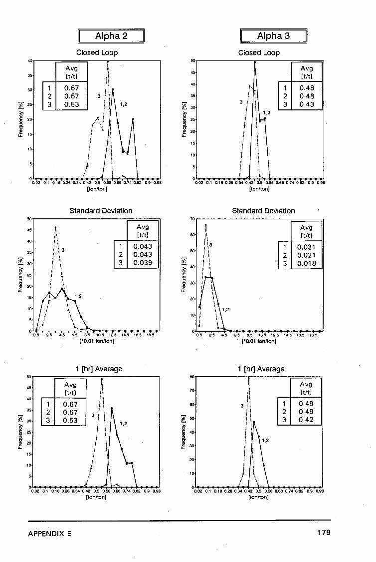
Univers

ity of

Cap

e Tow

n

~ >-0 c: Cl> :I C" :!! u.

'i: >-0 c: Cl> :I C" :!! u.

'i: >-0 c: Cl> :I

~ u.

40

35

30

25

20

15

10

5

0

1 2 3

Alpha 2

Closed Loop

Avg [t/t]

0.67 0.67 0.53

0.02 0.1 o. 18 0.28 0.34 0.42 0.5 0.58 0.86 0.74 0.82 0.9 0.98

[ton/ton]

50

45

40

35

30

25

20

50

45

40

35

30

25

20

15

10

5

0

Standard Deviation

Avg [t/t]

1 0.043 2 0.043 3 0.039

l \

U U U U U 1U 1U 1U 1U 1U

[*0.01 ton/ton]

1 [hr] Average

1 2 3

0.02 0.1 0. 18 0.26 0.34 0.42 0.5 0.58 0.88 0.74 0.82 0.9 0.98

[ton/ton]

APPENDIX E

Alpha 3

Closed Loop 50,--------,------;:::====il

45

40

35

~ 30

~ c: 25 ~ ~ 20 u.

15

10

5

T'·.

3 / \ I ; 1,2

j \H f l I \ : j : ;

! 1 : j : ~ : j

i i f 1

1 2 3

Avg [t/t]

0.48 0.48 0.43

o ...... .-. ______ ..... ,....,.:::;:.......~·~··....+ ........................................... ......i

0.02 0. 1 0. 18 0.28 0.34 0.42 0.5 0.58 0.88 0. 74 0.82 0.9 0.98

[ton/ton]

Standard Deviation 70r--------------;::::======::;i

80

50

20

10

Avg [t/t]

1 0.021 2 0.021 3 0.018

2.5 4.5 8.5 8.5 10.5 12.5 14.5 16.5 18.5

[*0.01 ton/ton]

1 [hr] Average ~.-------r------;:::=====::::;i

70

~ 50

~ Iii 40 :I

l 30

20

10

.I \ ' .~ \ i \

1 2 3

Avg [t/t)

0.49 0.49 0.42

/ \ o ...... .-.--.-. ................. t-T....,.......+--................................. _. 0.02 0. 1 o. 18 0.26 0.34 0.42 0.5 0.58 0.88 0.74 0.82 0.9 0.98

[ton/ton]

179

Univers

ity of

Cap

e Tow

n

Recycle

Closed Loop 40

I Avg

35 (%]

30 1 105 2 105

~ 25 3 89 >- 1,2 0 c 20 GI :::J

~ ' u.. 15

I 10

5 .~ .... /

0 5 25 45 85 85 105 125 145 185 185

Recycle[%]

Standard Deviation 35

/\ Avg

30 (%]

1 8 25 2 8

~ 3 15 >- 20 0 c GI :::J i \ ~

15 i \

u.. \

10 \

\ 5

• . , 0

............ ... 5 9 13 17 21 25 29 33 37

Recycle[%]

1 [hr] Average eo

• Avg !

50 n [%]

1 105

40 2 ·105

£. 3 88 ~ c: 30 1,2 GI :::J

~ u.. 20

I i

10 t /

0 /

5 25 45 85 85 105 125 1~ 185 185

Recycle[%]

APPENDIX E 180

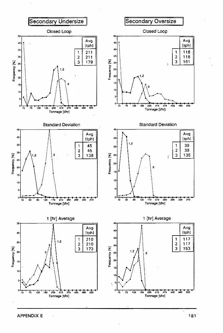
Univers

ity of

Cap

e Tow

n

Secondary Undersize llsecondary Oversize II Closed Loop Closed Loop

50 50

45 Avg

45 Avg

[tph] [tph] 40 40

1 211 1 118 35 2 211 35 2 118

~ 30 3 179 '£ 30 3 161 it

>-(,)

1,2 c: 25 c: 25 G) G) ::::i ::::i 1 CT 20 ~ 20 ...... u. u.

I .,,

15 \3 15

10 10 I \

\ 5 5 I \ · ................

\ 0 0 15 75 135 195 255 315 375 435 495 555

15 75 135 195 255 315 375 435 495 555 Tonnage [t/hr] Tonnage [t/hr]


Avg Avg 40

[tph] 35 [tph].

35 1 45 1,2 1 39 30

30 2 45 2 39 ~ 3 138 ~ 25 __ ,. ...... 3 135 >- 25 it (,) c: c: 20 G) G)

::::i 20 ::::i

1 1 15 u. u. 15

10 10

5 /: \ 5

\ !

0 0 .....

10 50 90 130 170 210 250 290 330 370 10 50 90 130 170 210 250 290 330 370


1 [hr) Average 1 [hr) Average 35 45

Avg 40 l: Avg

30 [tph]

/\, [tph]

1 210 35 1 117 25 1,2

2 210 2 117 1. 30

~ 3t 3 173 ~ 3 153 >- 20 >- 25 (,) \ (,) i c: i c: G)

\ G)

\ ::::i

I ::::i 20 ;

1 15 1 .. • \ ! u. /\\ u. i \ 15

10 ; \ I \ _..i ' \ i I

~~1 •., l'' l 5 ' i · ..... ,-' ' 5 • .. ,•'

t .. i \l i 0 0

15 75 135 195 255 315 375 435 495 555 15 75 135 195 255 315 375 435 495 555


APPENDIX E 181

Univers

ity of

Cap

e Tow

n

Tertiary Undersize

Closed Loop so.---------------;==::::::;i

1 50

.20

1.

,,_/t,

Avg [tph]

1 118 2 125 3 156

/;'•,, "·\ 10 \ .•

i I \ / \ ·· .... oJ..,.-_._...,... ....... ,___,,..--r-~.,._~•~·~·-~-~-..,.. ..... ....-..-J

15 75 135 195 255 315 375 435 495 555

Tonnage [t/hr]

Standard Deviation so,---------------;==::::::;i

50

20

10

Avg [tph)

1 41 2 120 3 40

10 50 90 130 170 210 250 290 330 370

Tonnage [t/hr]

1 [hr] Average so.---------------.====::::;,

45

40

35

~ 30

~ 5i 25 :I

l 20

15

10

f ~

/\, f \

\ i \ !

\

Avg [tph)

1 117 2 118 3 154

15 75 135 195 255 315 375 435 495 555

Tonnage [t/hr]

APPENDIX E

Tertiary Oversize

Closed Loop so.---------------;:::==::::;i

i 50

15 75 135 195 255 315 375

Tonnage [t/hr]

Avg [tph)

1 130 2 138 3 206

435 495 555

Standard Deviation 70.------------·====:;i

60

50

20

10

Avg [tph]

1 46 2 127 3 42

10 50 90 130 170 210 250 290 330 370

Tonnage [t/hr]

1 [hr] Average 40.----------------;;:::=====;i

35

30

10

1. !i

I\ i ! 3

I \ \ ' '

Avg, [tph]

1 129 2 130 3 205

\ ! i

5 \

0 ........ ....-....-~~~~-+-...... t-11,_....-e-______ ....... ._._..... 15 75 135 195 255 315 375 435 495 555

Tonnage [t/hr]

182

Univers

ity of

Cap

e Tow

n

ertiary Fee

Closed Loop Open Loop 35 45

Avg Comparison not meaningful here (scales different)

[tph]

f ~ 40

30 Graph just added for completeness

1 247 35

25 2 248 Avg 30 [tph]

'£ 3 361

I\ ~

20 !Plant >- >- 25 659 0 0 c: c:

C1l

'\ \ C1l

:I :I 20 tT 15 tT ~ ~

LL. i \ LL. ; ~ 15

10 : ~

i \

I\ \ 10

5 5 • ............. I) \ \

0 ·-··· 0 15 75 135 195 255 315 375 435 495 555 30 150 270 390 510 630 750 870 990 1110



3 .. 0:

Avg Avg 30 [tph]

25 [tph]

1 73 Plant 223 25 2 142

20

~ :; I \ 3 132 ~ I: I . >- 20

I~ I\ >-0 0 c: c: 15 C1l C1l :I :I

~ 15 f \j \ ~

u. u.

I \ 10 10 ~ i\ : /

5 5

! /

\ .. j / • ............. ;.../

....... ,.; .. .; . 0 0

10 50 90 130 170 210 250 290 330 370 10 50 90 130 170 210 250 290 330 370


1 (hr] Average 1 (hr] Average 35 40

Avg Avg 30 [tph] 35 [tph]

1 246 30 Plant 663 25 2 247

~ 3 358 [ 25

~ 20 >-

0 c: c: 20 C1l C1l :I :I

~ 15

~ u. : . u. 15

10

,1~::.J I\\ 10

5

...... ,. .............................. ···"···.» 5

IL.: 0 0

15 75 135 195 255 315 375 435 495 555 30 150 270 390 510 630 750 870 990 1110


APPENDIX E 183

Univers

ity of

Cap

e Tow

n

APPENDIX F

This appendix proves, using formulae of Chapter 3 relating feeds and screen split ratios

to secondary crusher gaps, that at a headfeed of 320[tph] the steady state values of the

simulator are:

GateE = Gatep = 0.29[t/t]

Feedc = Feed0 = 160[tph]

FeedE = Feedp = lOO[tph]

a 2 = 0.68[t/t]

a 3 = 0.S[t/t]

These values are the operating points needed to evaluate tertiary bin transfer functions.

If the headfeed is 320[tph], each secondary crusher has to pass 160[tph]. Using the

relation between secondary crusher gaps and secondary feed (Chapter 3, §3.2.3(c)), a

value of 19.2[mm] is obtained for the secondary crusher gaps.

Secondary and tertiary screen split ratios are then (Chapter 3, §3.2.3(b)):

a 2 = 0.68[t/t]

a 3 = O.SO[t/t]

and therefore the secondary oversize is lOO[tph]. For steady state, combined tertiary

crusher undersize must be lOO[tph], and using a 3 = 0.5 gives a tertiary crusher feed of '

lOO[tph] each.

If tertiary gates are fully open, tertiary crusher feed will be 340[tph]. Therefore, the

tertiary gates need to be closed to 100/340 = 0.29[t/t] so that only lOO[tph] of material

goes to each tertiary crusher.

The same values are obtained by running the simulator to steady state with a headfeed

of 320[tph].

APPENDIX F 184

Univers

ity of

Cap

e Tow

n

APPENDIX G

The simulation software is contained on the diskette at the bottom of the page. To run

the simulator, copy the files sim.exe, sim.cfg and egavga.bgi (<0 Borland International) to

a local directory. Note that the simulator requires read/write access to the current

directory. Then type sim to start, and follow the instructions in Chapter 5.

Other files on the diskette contain source code for the simulator. To recompile,

Borland C + + v2.0 or later is required. Open a project window from the main menu and

include all files with .cpp and .c extensions, and then compile. It should compile under a

small model, but if errors are reported, try using a medium model

(Options/Compiler/Code Generation). There should be no difficulties.

APPENDIX G

For the software, please contact:

Professor M Braae

Department of Electrical and Electronic Engineering

University of Cape Town

Private Bag

Rondebosch

7700

Republic of South Africa

Fax: (South Africa) + 21 650-3465

Email: [email protected]

185

a feasibility study for an imc application in the mining ... stage at a mine. first, a mathematical...

Documents