A Framework for Measurement Error in Self-Reported Health Conditions

Ling Li and Perry Singleton

Paper No. 191 August 2016

CENTER FOR POLICY RESEARCH –Summer 2016

Leonard M. Lopoo, Director Professor of Public Administration and International Affairs (PAIA)

Associate Directors Margaret Austin

Associate Director, Budget and Administration

John Yinger Trustee Professor of Economics and PAIA Associate Director, Metropolitan Studies

SENIOR RESEARCH ASSOCIATES

Badi Baltagi, Economics Robert Bifulco, PAIA Leonard Burman, PAIA Thomas Dennison, PAIA Alfonso Flores-Lagunes, Economics Sarah Hamersma, PAIA William C. Horrace, Economics Yilin Hou, PAIA Hugo Jales, Economics

Duke Kao, Economics Jeffrey Kubik, Economics Yoonseok Lee, Economics Amy Lutz, Sociology Yingyi Ma, Sociology Jerry Miner, Economics Cynthia Morrow, PAIA Jan Ondrich, Economics John Palmer, PAIA David Popp, PAIA

Stuart Rosenthal, Economics Michah Rothbart, PAIA Rebecca Schewe, Sociology Amy Ellen Schwartz, PAIA/Economics Perry Singleton, Economics Michael Wasylenko, Economics Peter Wilcoxen, PAIA

GRADUATE ASSOCIATES

Emily Cardon, PAIA Carlos Diaz, Economics Alex Falevich, Economics Wancong Fu, Economics Boqian Jiang, Economics Hyunseok Jung, Economics Yusun Kim, PAIA Ling Li, Economics

Michelle Lofton, PAIA Judson Murchie, PAIA Brian Ohl, PAIA Jindong Pang, Economics Laura Rodriquez-Ortiz, PAIA Fabio Rueda De Vivero, Economics David Schwegman, PAIA

Shulin Shen, Economics Iuliia Shybalkina, PAIA Kelly Stevens, PAIA Saied Toossi, PAIA Rebecca Wang, Sociology Xirui Zhang, Economics

STAFF

Kelly Bogart, Administrative Specialist Kathleen Nasto, Administrative Assistant Candi Patterson, Computer Consultant

Mary Santy, Administrative Assistant Katrina Wingle, Administrative Assistant

Abstract

This study develops and estimates a model of measurement error in self-reported

health conditions. The model allows self-reports of a health condition to differ from a

contemporaneous medical examination, prior medical records, or both. The model is estimated

using a two-sample strategy, which combines survey data linked medical examination results

and survey data linked to prior medical records. The study finds substantial inconsistencies

between self-reported health, the medical record, and prior medical records. The study

proposes alternative estimators for the prevalence of diagnosed and undiagnosed conditions

and estimates the bias that arises when using self-reported health conditions as explanatory

variables.

JEL No. I12, J22

Keywords: Measurement Error, Disease Prevalence, Diabetes, Hypertension

Author: Ling Li, Department of Economics, Center for Policy Research, Syracuse University, 426 Eggers Hall, Syracuse, NY 13244 (315) 443-9056; Lli37@syr.edu

Corresponding Author: Perry Singleton; Associate Professor, Department of Economics; Senior Research Associate, Center for Policy Research; Syracuse University. Contacts: 426 Eggers Hall; Syracuse University, Syracuse, NY 13244; (315) 443-3114; psinglet@syr.edu.

The authors would like to thank John Cawley, Gary Engelhardt, Alfonso Flores-Lagunes, Bruce

Meyer, Jeffrey Kubik, Yoonseok Lee, and seminar participants at Cornell University for valuable

comments.

I. Introduction

Several surveys collect data on previously diagnosed health conditions, and these data

are used for in a variety of applications, from estimating the prevalence of health conditions to

estimating the effect of health conditions on labor market outcomes. However, several recent

studies question the validity of self-reported health conditions. For example, Baker, Stabile,

and Deri (2004) link survey data to prior medical records and find substantial inconsistencies

between self-reported health conditions and the medical record. Additionally, Johnston,

Propper, and Shields (2009) use survey data linked to results from a medical examination and

find substantial inconsistencies between self-reported hypertension and a clinical test. These

inconsistencies lead to measurement error, which not only bias the estimated prevalence of

health conditions, but also the correlation between health conditions and other outcomes of

interest.1

To validate data on self-reported health conditions for the US, some studies use survey

data linked to medical records, while others use survey data linked to a medical examination.2

Currently, no study uses survey data linked to both the medical record and a medical

examination, as no such data linkage exists. To address this shortcoming, this study proposes a

two-sample estimation strategy. The study first develops a model of measurement error in

self-reported health conditions. The model is composed of three binary variables: an indicator

1 For a reviews of measurement error in survey data, see Bound, Brown, and Mathiowetz (2001) and Meyer, Mok, and Sullivan (2015). 2 Studies that validate self-reported health or health behaviors using administrative data include Madow (1973); Martin et al. (2000); and Suziedelyte and Johar (2013). Studies that validate self-reported health conditions using medical examination results include Butler, Burkhauser, Mitchell, and Pincus (1987), Cawley and Choi (2015), and Johnston, Propper, and Shields (2009)

4

of the self-report, an indicator of the medical examination result, and an indicator of the

medical record. With three binary variables, the joint probability distribution consists of eight

population moments. The study then estimates these moments using two separate data

linkages: survey data linked to medical records and survey data linked to medical exam results.

The latter come from the study Baker, Stabile, and Deri (2004), who use the Canadian National

Population Health Survey linked to the Ontario Health Insurance Plan (OHIP). The former

comes from the National Health and Nutrition Examination Survey. Given the available data,

the analysis focuses on two conditions: hypertension and diabetes.

The study yields several results. First, the study provides an alternative estimate for the

prevalence of undiagnosed health conditions. In many studies, undiagnosed conditions are

defined as those that are not self-reported at the time of the survey, but are detected upon

medical examination.3 However, this definition may overstate the prevalence of undiagnosed

conditions if individuals had been previously diagnosed – and thus have a medical record – but

simply fail to report the condition at the time of the survey. After accounting for this

possibility, the prevalence of undiagnosed hypertension decreases from 9.0 percent to 2.4

percent, and the prevalence of undiagnosed diabetes decreases from 2.7 percent to 1.3

percent.

Second, the study provides an alternative estimate for the prevalence of diagnosed

health conditions. In many studies, diagnosed conditions are defined as those that are self-

reported, regardless of whether they test positive for the condition at the time of the survey.

3 For example, Cowie et al (2006) estimate that approximately 2.8 percent of the population in 2002 had undiagnosed diabetes, and Sug Yoon et al (2012) estimate that approximately 5.2 percent of the population in 2009 had undiagnosed hypertension.

5

While this may be plausible for individuals whose health had improved, this may also reflect

individuals who were never formally diagnosed, but report the condition nonetheless, perhaps

to justify non-employment or eligibility for disability benefits.4 After accounting for this

possibility, the prevalence of diagnosed hypertension decreases from 20.0 percent to 15.5

percent, and the prevalence of diagnosed diabetes decreases from 6.0 percent to 5.0 percent.

Third, the study examines the bias that may arise when estimating the causal effect of

health conditions on other outcomes of interest, such as labor supply.5 In a simplified model,

the bias is proportional to 𝑐𝑜𝑣(𝑆, 𝑢)/𝑣𝑎𝑟(𝑆), where 𝑆 is the self-reported variable and 𝑢 is the

measurement error.6 The proportional bias is estimated for various definitions of true health

using the estimated distribution of measurement error. According to the calculations, the

proportion bias ranges from 0.308 to 0.710 for hypertension from 0.187 to 0.363 for diabetes.

The bias is smallest when true health is defined by the medical record only and greatest when

true health is defined by the medical examination only.

The results underscore the potential biases that may arise when using self-reported

health conditions. A notable limitation is that, to estimate measurement error, the study

employs a two-sample strategy using data from Canada and the US. Ideally, survey data would

be linked to both medical records and medical examinations, obviating the need for the two-

4 Studies that examine the endogeneity of self-reported health include Bound (1991); Dwyer and Mitchell (1999); and Benitez-Silva, Buchinsky, Chan, Cheidvasser, and Rust (2004). 5 Currie and Madrian (1999) raise concern for undiagnosed health conditions when estimating the effect of health on labor market outcomes. However, it remains unclear how undiagnosed health conditions affect work capacity, or how selection into medical screening affects the association between self-reported health and labor market outcomes. 6 For a more technical discussion of measurement error, see Bound, Brown and Mathiowetz (2001).

6

sample strategy. And, when using two-sample strategy, the data would ideally represent the

same populations. However, there is no representative survey of the US that links survey data

to comprehensive medical records. Thus, this study is the first reasonable attempt to estimate

measurement error in self-reported health conditions – relative to both the medical record and

medical examination – given the available data.

II. Methodology

A. Model of Measurement Error

The empirical objective is to determine whether self-reports of specific health

conditions are consistent with a contemporaneous medical examination or prior medical

records. This is accomplished in two steps. The first step is to specify a population-level model

of measurement error, which specifically allows the self-report of a health condition to differ

from a medical examination, prior medical records, or both. The second step is to estimate the

moments of the model using population-based survey data.

The model of measurement error consists of three binary variables. The first variable is

a self-report of a previous diagnosis for the condition: the variable equals one if a survey

participant reports a previous diagnosis and zero otherwise. The second variable is the result of

a medical examination at the time of the survey: the variable equals one if a survey participant

tests positive for the condition and zero otherwise. The third variable is an indicator of the

medical record: the variable equals one if the survey participant has a medical record of the

condition and zero otherwise.

With three binary variables, the joint probability distribution consists of eight moments.

The joint probability distribution is given by the following table:

7

Medical Examination (E)

Self-Report (S) No (E=0) Yes (E=1)

No (S=0) 𝜋00 = 𝜋000 + 𝜋001 𝜋01 = 𝜋010 + 𝜋011

Yes (S=1) 𝜋10 = 𝜋100 + 𝜋101 𝜋11 = 𝜋110 + 𝜋111

The rows correspond to the self-report, and the columns correspond to the medical

examination. These two variables yield four population moments, denoted 𝜋𝑆𝐸 . The first

subscript corresponds to the value of the self-report, and the second subscript corresponds to

the value of the medical examination. For example, 𝜋00 represents the percent of the

population who do not self-report the condition and who do not test positive for the condition

at the time of the survey. To incorporate the medical record, each 𝜋𝑆𝐸 is disaggregated into

those with and without a medical record, denoted 𝜋𝑆𝐸𝑅. Thus, 𝜋000 represents the percent of

the population who do not self-report the condition, who do not test positive for the condition

at the time of the survey, and who do not have medical record of the condition.

The model has three important empirical applications. First, the model highlights the

difficulty in defining and measuring the prevalence of undiagnosed health conditions. To

measure prevalence, several studies define undiagnosed conditions as those that are not self-

reported at the time of the survey, but are detected upon medical examination. This case

corresponds to 𝜋01 in the model above. However, 𝜋01 may include individuals who had been

previously diagnosed, and thus have a medical record, but who fail to report the condition at

the time of the survey. This occurs with probability 𝜋011. An important consideration is

8

whether 𝜋011 should be excluded from estimates of undiagnosed health conditions. If so,

prevalence of undiagnosed conditions should be measured as 𝜋010, rather than 𝜋01.

Second, the model highlights the difficulty in defining and measuring the prevalence of

diagnosed health conditions. To measure prevalence, several studies define diagnosed

conditions as those that are self-reported, regardless of whether they test positive for the

condition at the time of the survey. This case corresponds to 𝜋11 + 𝜋10 in the model above.

However, the latter term may include individuals who were never formally diagnosed, but

report the condition nonetheless, perhaps to justify non-employment or eligibility for disability

benefits. This occurs with probability 𝜋010. An important consideration is whether 𝜋010 should

be excluded from estimates of diagnosed health conditions. If so, the prevalence of diagnosed

conditions should be measured as 𝜋11 + 𝜋101, rather than 𝜋11 + 𝜋10.

Third, the model helps to characterize the biases that may arise when using self-

reported health conditions as explanatory variables. For example, a structural model of an

outcome 𝑌 as a function of health condition 𝑆∗ is given by the following equation:

(1) 𝑌 = 𝛽0 + 𝛽1𝑆∗ + 휀.

For example, the model may be used to examine the causal effect of a health condition 𝑆∗ on

labor supply 𝑌. The causal effect is denoted by the parameter 𝛽1. The variable 𝑆∗ is defined by

the states of health that do and do not affect the outcome. For example, 𝑆∗ may be defined by

the result of a medical examination, regardless of whether the condition had been previously

diagnosed or self-reported, as in Johnston, Propper, and Shields (2009). Alternatively, 𝑆∗ may

be defined solely by the medical record, as in Baker, Stabile, and Deri (2004). Another

9

possibility is that the 𝑆∗ is measured by a combination of a medical examination and the

medical record.

When true health 𝑆∗ is replaced with self-reported health, denoted 𝑆, the estimate of 𝛽1

may be biased. To characterize the bias, the self-report of the health condition is expressed as

the sum of 𝑆∗ and an error term 𝑢: 𝑆 = 𝑆∗ + 𝑢. When 𝑆∗ is substituted in (1), the equation

becomes

(2) 𝑌 = 𝛽0 + 𝛽1𝑆 + 휀 − 𝛽1𝑢.

By construction, 𝑆 is correlated with 𝑢. If 휀 is uncorrelated with 𝑆∗ and 𝑢, then the least

squares estimate of 𝛽1 converges in probability to 𝛽1[1 − 𝑐𝑜𝑣(𝑆, 𝑢)/𝑣𝑎𝑟(𝑆)]. Thus, the bias

due to measurement error is proportional to 𝑐𝑜𝑣(𝑆, 𝑢)/𝑣𝑎𝑟(𝑆). This bias may be estimated

given a definition of true health 𝑆∗ and values for the eight population moments 𝜋𝑆𝐸𝑅.

B. Data and Estimation Strategy

To estimate the eight population moments 𝜋𝑆𝐸𝑅 , the study would ideally use survey

data matched to both medical examination results and medical records. However, no such data

exist for a representative sample of the US population. As an alternative, this study uses two

separate data linkages: survey data linked to medical records, and survey data linked to medical

exam results. Intuitively, the joint distribution is composed of several moments. Some

moments can be estimated using survey data linked to medical records; others can be

estimated from survey data linked to medical exam results. These estimates, combined, yield

the underlying joint distribution 𝜋𝑆𝐸𝑅 in the population.

Survey data linked to medical examinations come from the National Health and

Nutrition Examination Survey (NHANES). The NHANES was designed, in part, to estimate the

10

prevalence of undiagnosed health conditions in the US population. This is accomplished by first

asking participants if they have ever been diagnosed for certain health conditions by a medical

professional, and then testing participants for these conditions by medical examination. These

data are used two estimate four population moments 𝜋11, 𝜋00, 𝜋10, and 𝜋01.

Information on survey data linked to medical records comes from a study by Baker,

Stabile, and Deri (2004). The study examines whether self-reported health conditions in survey

data are consistent with previous medical records. The survey data come from 1996/1997

version of the Canadian National Population Health Survey (CNPHS), and the data from medical

record come from the Ontario Health Insurance Plan (OHIP). The study is limited to Ontario, as

the OHIP data come from Ontario only. As the authors state, OHIP records provide a

comprehensive view of previous health services, as alternative services are either expensive or

prohibited.

Using these data, the authors find substantial inconsistencies between self-reported

health and the medical record. To characterize these inconsistencies, the authors calculate

rates of false-negatives and false-positives for various health conditions. The rate of false-

negatives is defined as the percent of individuals who fail to self-report a medical condition,

conditional on having a medical record for the condition. Conversely, the rate of false-positives

is defined as the percent of individuals who self-report a medical condition, conditional on

having no medical record for the condition. They find that, for many conditions, more than 50

percent of individuals who have a medical record for a condition fail to report it in the survey.

Rates of false-positive reporting are considerably lower.

11

The estimated rates of false-negative and false-positive reporting are used to identify

population moments of the model above. To link the two, the rate of false-negative reporting

is expressed as,

𝑅𝐹𝑁 =𝜋001+𝜋011

𝜋001+𝜋111+𝜋101+𝜋011.

Similarly, the rate of false-positive reporting is expressed as,

𝑅𝐹𝑃 =𝜋110+𝜋100

𝜋000+ 𝜋110+𝜋100+𝜋010.

The study by Baker, Stabile, and Deri (2004) provides estimates of 𝑅𝐹𝑁 and 𝑅𝐹𝑃.

The model contains eight population moments, but the data thus far provide only six:

𝜋11, 𝜋00, 𝜋10, 𝜋01, 𝑅𝐹𝑁, and 𝑅𝐹𝑁. Thus, to identify the joint distribution, two additional

assumptions are made. The first assumption is that 𝜋00 = 𝜋000, so that 𝜋001 = 0. Intuitively,

individuals who do not self-report a condition and do not test positively for the condition by

medical examination are assumed to have no medical record of the condition. The second

assumption is that 𝜋11 = 𝜋111, so that 𝜋110 = 0. Intuitively, individuals who self-report a

condition and test positively for the condition by medical examination are assumed to have a

medical record of the condition. Both assumptions rely on the medical examination (𝐸) to

validate self-reported health (𝑆), which implies whether a medical record (𝑅) should or should

not exist.

With six estimates and two assumptions, the eight population moments 𝜋𝑆𝐸𝑅 are

identified. Details of the calculation and estimation are provided in the Appendix.

The identification strategy requires the rates 𝑅𝐹𝑁 and 𝑅𝐹𝑃 to be the same between the

NHANES and the NPHS/OHIP. For this assumption to be credible, it is important that the data

are comparable. The CNPHS/OHIP data come from years 1996/1997. Thus, the analysis uses

12

NHANES data from calendar years 1999, the first year of data, to 2003. The sample in Baker,

Stabile, and Deri (2004) is restricted to individuals who are aged 16 and not attending school.

The NHANES is similarly restricted. The NHANES oversamples certain groups, so all estimations

use sample weights.

An obvious concern is that the NHANES is representative of the US, whereas the CNPHS

and OHIP are representative of Ontario. While not ideal, the few US-based studies that validate

self-reported health conditions using medical records (Harlow and Linet 1989) are limited in

scope. For example, Martin et al (2000) focus on enrollees of a single insurance firm, and

medical records come from claims within the firm.

Another concern pertains to the survey questions of health conditions. In the NHANES,

survey participants are asked, “[Have you] ever been told by a doctor or other health

professional that [you have] [this condition]?” In the CNPHS, survey participants are asked, “Do

[you] have any of the following long-term conditions that have been diagnosed by a healthcare

professional?”.7 While both questions ask about health conditions diagnosed by medical

professionals, the question in the CNPHS may be interpreted in the present tense, whereas the

question in the NHANES may be interpreted in past tense. This difference may result in lower

prevalence rates in the CNPHS, which would result in a higher 𝑅𝐹𝑁 and lower 𝑅𝐹𝑃 relative to the

NHANES.

Given the available data, the analysis focuses on two health conditions: hypertension

and diabetes. In the NHANES, survey participants are first asked whether they have been

7 “Healthcare professional” is defined to exclude alternative healthcare providers, such as acupuncturists, and “long-term” is defined as a condition that is expected to last six months or more.

13

previously diagnosed for hypertension and diabetes, and then are tested for these conditions

by medical examination. For hypertension, the self-report variable 𝑆 equals one if the survey

participant had been diagnosed at least twice for hypertension by a medical professional, and

the medical exam variable 𝐸 equals one if the survey participant tests positive for hypertension

based the on the average of up four blood pressure readings.8 For diabetes, the self-report

variable 𝑆 equals one if the survey participant had been diagnosed for diabetes, and the

medical exam variable 𝐸 equals one if the survey participant tests positive for diabetes based

on a test of fasting plasma glucose.9 In regards to 𝑅𝐹𝑁 and 𝑅𝐹𝑃, Baker, Stabile, and Deri (2003)

report multiple estimates based on various specifications of the medical record. The

specification used in this study requires at least two OHIP records for a specific condition during

the two years prior to the survey.

III. Results

A. Estimates of Joint Distribution: 𝝅𝑺𝑬𝑹

Table 1 presents estimates of 𝑅𝐹𝑁, 𝑅𝐹𝑃, and 𝜋𝑆𝐸𝑅 for hypertension and diabetes. The

first two columns report estimates of 𝑅𝐹𝑁 and 𝑅𝐹𝑃, derived from Baker, Stabile, and Deri

(2004). For both conditions, the rate of false-negative reporting ranges between 20 and 30

percent. This suggests that many people who have a medical record for a condition, and thus

may test positive for the condition by medical examination, may fail to report the condition

8 A diagnosis of hypertension is based on blood pressure readings of both systolic and diastolic pressure. Hypertension is defined as systolic greater than or equal to 140 mm Hg or diastolic greater than or equal to 90 mm Hg. 9 The test for fasting plasma glucose is administered to only half of the sample. Diabetes is defined as fasting plasma glucose greater than or equal to 126 mg/dl.

14

nonetheless. The rate of false-positive reporting is much lower, ranging from 1 to 6 percent.

This suggests that few individuals falsely claim or self-diagnose a condition.

The next four columns report estimates for 𝜋11, 𝜋00, 𝜋10, and 𝜋01. These estimates are

derived solely from the NHANES. As shown, only 40.3 percent of those who self-report

hypertension actually test positive for hypertension by medical examination

(𝜋11 (𝜋11 + 𝜋10)⁄ ). Conversely, only 47.3 percent of those who test positive for hypertension

by medical examination actually self-report hypertension (𝜋11/(𝜋11 + 𝜋01)). These figures for

diabetes are 66.5 percent and 60.1 percent, respectively. Based solely on 𝜋01, the prevalence

of undiagnosed hypertension and diabetes is 9.0 percent and 2.7 percent, respectively.

The final four columns disaggregate 𝜋10 and 𝜋01 into those with and without a medical

record. In regards to 𝜋01, the empirical question is whether individuals who test positive for

the condition, but fail to self-report it, have a medical record for the condition nonetheless. As

shown, an estimated 72.8 percent of individuals who test positive for hypertension, but fail to

report it, have a medical record for hypertension (𝜋011/(𝜋010 + 𝜋011)). This figure for

diabetes is 50.1 percent. If 𝜋011 should be excluded from estimates of undiagnosed conditions,

then the prevalence of hypertension is closer to 2.4 percent (𝜋010) than 9.0 percent (𝜋01), and

the prevalence of diabetes is closer to 1.3 percent than 2.7 percent.

In regards to 𝜋10, the empirical question is whether individuals who self-report a

condition, but do not test positive for the condition by medical examination, have a medical

record for the condition. As shown, an estimated 62.2 percent of individuals who self-report

hypertension, but do not test positive for hypertension by medical examination, have a medical

record (𝜋101/(𝜋100 + 𝜋101)). This figure for diabetes is 48.4 percent. If 𝜋100 should be

15

excluded from estimates of diagnosed conditions, then the prevalence of hypertension is closer

to 15.5 percent (𝜋11 + 𝜋101) than 20.0 percent (𝜋100 + 𝜋10), and the prevalence of diabetes is

closer to 5.0 percent than 6.0 percent.

B. Estimates of Proportional Bias: 𝒄𝒐𝒗(𝑺, 𝒖)/𝒗𝒂𝒓(𝑺)

Stated above, the model of measurement error helps to characterize the biases that

may arise when using self-reported health conditions as explanatory variables. Specifically, if

𝛽1 is the causal effect of true health 𝑆∗ on outcome 𝑌, and if 𝑆∗ is replaced with self-reported

health 𝑆, then the estimate of 𝛽1 converges in probability to 𝛽1[1 − 𝑐𝑜𝑣(𝑆, 𝑢)/𝑣𝑎𝑟(𝑆)]. Thus,

the bias due to measurement error is proportional to 𝑐𝑜𝑣(𝑆, 𝑢)/𝑣𝑎𝑟(𝑆).

Given estimates 𝜋𝑆𝐸𝑅 , the proportional bias term 𝑐𝑜𝑣(𝑆, 𝑢)/𝑣𝑎𝑟(𝑆) is estimated for

various definitions of true health 𝑆∗. These estimates are presented in Table 2. The

calculations for hypertension are reported in the first panel, and the calculations for diabetes

are reported in the second panel. Each panel contains four rows, corresponding to different

definitions of 𝑆∗.

In the first row, 𝑆∗ is defined by the medical record only. In this case, measurement

error 𝑢 equals 𝑆 − 𝑅. Based on the estimates of 𝜋𝑆𝐸𝑅 , the next four columns report estimates

of the mean of 𝑆, variance of 𝑆, mean of 𝑢, and covariance of 𝑆 and 𝑢. The final column reports

the proportional bias. As shown, the bias is 0.308 for hypertension and 0.187 for diabetes.

These estimates are similar to Baker, Stabile, and Deri (2003), who estimate a proportional bias

of 0.355 for hypertension and 0.195 for diabetes.

In the second row, 𝑆∗ is defined by the medical examination only. In this case,

measurement error 𝑢 equals 𝑆 − 𝐸. As shown, the proportional bias is considerably greater,

16

reaching 0.710 for hypertension and 0.363 for diabetes. The estimate for hypertension is

similar to the estimate by Johnston, Propper, and Shields (2009), who use survey data matched

to medical examinations from the Health Survey for England.10 They estimate a proportional

bias for hypertension of 0.68.

In the third and fourth rows, 𝑆∗ is defined by a combination of the medical record and

the medical examination. In the third row, true health is defined by either the medical record

or the examination; in the fourth row, true health requires both a medical record and a positive

result by medical examination. As shown, the estimates of proportional bias fall between the

estimates in the first and second rows.

Thus, the proportional bias is smallest when 𝑆∗ is defined by the medical record and

largest when 𝑆∗ is defined by the medical examination. The results reflect that, in the former

case, only two sources of measurement error exist: 𝜋100 and 𝜋011. However, in the latter case,

two additional sources of error arise: 𝜋101 and 𝜋010. These two additional sources of error

necessarily increase the proportional bias term 𝑐𝑜𝑣(𝑆, 𝑢)/𝑣𝑎𝑟(𝑆).

C. Sensitivity to Assumptions 𝝅𝟎𝟎 = 𝝅𝟎𝟎𝟎 and 𝝅𝟏𝟏 = 𝝅𝟏𝟏𝟏

To identify the joint distribution 𝜋𝑆𝐸𝑅, it was assumed that 𝜋00 = 𝜋000 and 𝜋11 = 𝜋111,

which imply that 𝜋001 = 0 and 𝜋110 = 0, respectively. Although both assumptions are

reasonable, an important question is whether the estimates of 𝜋𝑆𝐸𝑅 are sensitive to these

assumptions. To relax these assumptions, it is assumed that a share 𝛾 of 𝜋00 instead has a

medical record, so 𝜋001 = 𝛾𝜋00 and 𝜋000 = (1 − 𝛾)𝜋00. Similarly, it is assumed a share 𝛿 of

10 A similar analysis is conducted for arthritis by Butler, Burkhauser, Mitchell, and Pincus (1987).

17

𝜋11 instead does not have a medical record, so 𝜋110 = 𝛿𝜋11 and 𝜋111 = (1 − 𝛿)𝜋11. In the

baseline results presented above, the shares 𝛾 and 𝛿 were assumed zero.

In this case, the rate of false-negative reporting is expressed as,

𝑅𝐹𝑁 =𝛾𝜋00+𝜋011

𝛾𝜋00+(1−𝛿)𝜋11+𝜋101+𝜋011.

Similarly, the rate of false-positive reporting is expressed as,

𝑅𝐹𝑃 =𝛿𝜋11+𝜋100

(1−𝛾)𝜋00+ δ𝜋11+𝜋100+𝜋010.

The empirical question is whether the estimates of 𝜋𝑆𝐸𝑅 differ for various values of 𝛾 and 𝛿.

The calculations of 𝜋𝑆𝐸𝑅, described in the Appendix, yield two findings. First, the

estimates of 𝜋011 and 𝜋010 depend only on 𝛾, not 𝛿. Stated above, 𝜋01 has been interpreted as

the prevalence of undiagnosed health conditions, and 𝜋011 is the prevalence of these

conditions that had indeed been diagnosed, according to the medical record. The finding

suggests that the disaggregation of 𝜋01 into those with and without a medical record does not

require 𝛿 = 0 (𝜋110 = 0).

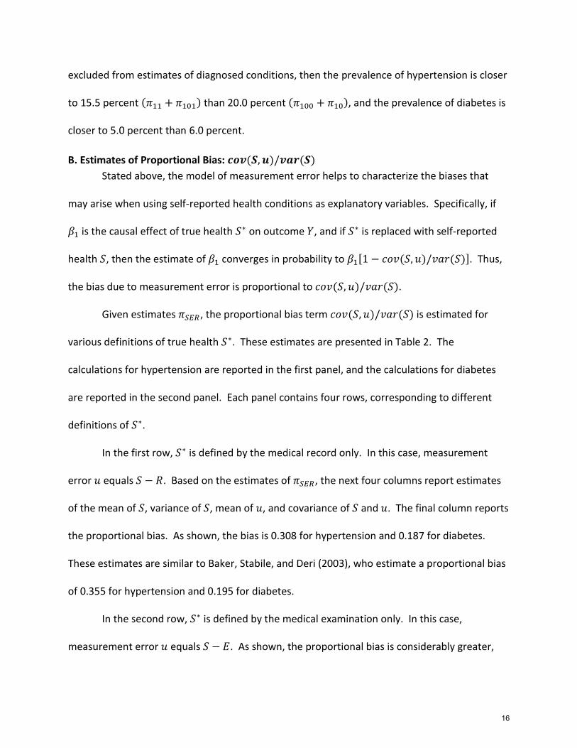
The sensitivity of 𝜋011 and 𝜋010 to different values of 𝛾 is given in panel A of Figures 1

and 2. The estimates for hypertension are presented in Figure 1, and the estimates for diabetes

are presented in Figure 2. Each panel graphs the estimates of 𝜋011 and 𝜋010 based on the value

of 𝛾, ranging from 0 to 0.05.

As shown, the estimates of 𝜋011 and 𝜋010 are sensitive to the value of 𝛾. In regards to

hypertension, the estimate of 𝜋011 decreases from 6.5 percent when 𝛾 equals zero to 3.0

percent when 𝛾 equals 0.05. As a result, the share of 𝜋01 with a medical record decreases from

72.85 percent to 33.7 percent (𝜋011 𝜋01⁄ ). The estimates of for diabetes appear more

18

sensitive. As shown, the estimate of 𝜋011 decreases quickly from 1.3 percent when 𝛾 equals

zero to zero when 𝛾 reaches approximately .015.

The second finding is that the estimates of 𝜋101 and 𝜋100 depend only on 𝛿, not 𝛾. The

term 𝜋10 pertains to individuals who self-report a condition, but do not test positive for the

condition by medical examination. The term 𝜋101 includes individuals who had been diagnosed

for the condition by a medical professional, accurately self-report the diagnosis during the

survey, but perhaps recovered from the condition at the time of the survey. The finding

suggests that the disaggregation of 𝜋10 into those with and without a medical record does not

require 𝛾 = 0 (𝜋001 = 0).

The sensitivity of 𝜋011 and 𝜋010 to different values of 𝛿 is given in panel B of Figures 1

and 2. As shown, the estimates of 𝜋011 and 𝜋010 appear less sensitive to the value of 𝛿. In

regards to hypertension, the estimate of 𝜋101 increases from 7.4 percent when 𝛿 equals zero to

7.8 percent when 𝛿 equals 0.05. As a result, the share of 𝜋10 with a medical record increases

from 62.2 percent to 65.5 percent (𝜋101 𝜋10⁄ ). The estimates of for diabetes also appear less

sensitive. As shown, the estimate of 𝜋011 increases from 1.0 percent when 𝛿 equals zero to 1.2

percent when 𝛿 reaches 0.05.

IV. Discussion and Conclusion

This study develops and estimates a model of measurement error in self-reported

health conditions. The model allows self-reports of a health condition to differ from a

contemporaneous medical examination, prior medical records, or both. The model is estimated

using a two-sample strategy, which combines survey data linked medical examination results

19

and survey data linked to prior medical records. The study finds substantial inconsistencies

between self-reported health, the medical record, and prior medical records.

The study has three empirical applications. First, the study provides an alternative

estimator of undiagnosed health conditions. Several studies define undiagnosed conditions as

those that are not self-reported at the time of the survey, but are detected upon medical

examination. The alternative estimator excludes those that are not self-reported, but are

included in the medical record nonetheless. Using the alternative estimator, the prevalence of

undiagnosed hypertension decreases from 9.0 percent to 2.4 percent, and the prevalence of

undiagnosed diabetes decreases from 2.7 percent to 1.3 percent.

Second, the study provides an alternative estimator of diagnosed conditions. Several

studies define diagnosed conditions as those that are self-reported, regardless of whether it is

detected upon medical examination. The alternative estimator excludes those that are self-

reported, are not reported upon medical examination, and not included in the medical record.

Using this alternative estimator, the prevalence of diagnosed hypertension decreases from 20.0

percent to 15.5 percent, and the prevalence of diagnosed diabetes decreases from 6.0 percent

to 5.0 percent.

Finally, the study examines the bias that may arise when estimating the causal effect of

health conditions on other outcomes of interest. In a simplified model, the proportional bias is

greatest when true health is defined by the medical examination only. In this case, the

proportional bias is 0.710 for hypertension and 0.363 for diabetes.

Using a two-sample strategy, this study is the first reasonable attempt to estimate

measurement error in self-reported health conditions relative to both the medical record and

20

medical examination. However, the estimation strategy has two notable limitations. First, this

study utilizes data from Canada and the US, which raises concerns about the comparability of

the two populations. Second, the estimation strategy requires assumptions about specific

population parameters – specifically 𝜋001 = 0 and 𝜋110 = 0. While these assumptions are

reasonable, it is imperative to test these assumptions empirically. These limitations can be

addressed using survey data linked to both medical examination results and medical records,

once such data become available.

21

Appendix

The empirical objective is to estimate the joint probability distribution of three binary variables: an indicator of a self-reported health condition, an indicator of the result from a medical examination, and an indicator of the medical record. The joint probability distribution is denoted 𝜋𝑆𝐸𝑅, where the three subscripts correspond to the three binary variables.

The joint distribution is estimated from two separate data linkages. The first is survey data linked to results from a medical examination. These data provide estimates of 𝜋11, 𝜋00, 𝜋10, and 𝜋01. The second is survey data linked to medical records. These data provide estimates of rates of false-negative and false-positive reporting, given by

𝑅𝐹𝑁 =𝜋001+𝜋011

𝜋001+𝜋111+𝜋101+𝜋011,

and

𝑅𝐹𝑃 =𝜋110+𝜋100

𝜋000+ 𝜋110+𝜋100+𝜋010,

respectively.

To identify the system, two additional assumptions are made. The first assumption is 𝜋00 = 𝜋000, so that 𝜋001 = 0. The second assumption is 𝜋11 = 𝜋111, so that 𝜋110 = 0. Both assumptions rely on the medical examination (𝐸) to validate self-reported health (𝑆), which implies whether a medical record (𝑅) should or should not exist.

With six estimates and two assumptions, the system is identified. Specifically,

𝜋011 =�̃�𝐹𝑁(𝜋11+𝜋10)−�̃�𝐹𝑁�̃�𝐹𝑃(𝜋00+𝜋01)

1−�̃�𝐹𝑁�̃�𝐹𝑃,

and

𝜋100 =�̃�𝐹𝑃(𝜋00+𝜋01)−�̃�𝐹𝑁�̃�𝐹𝑃(𝜋11+𝜋10)

1−�̃�𝐹𝑁�̃�𝐹𝑃.

Additionally, 𝜋010 = 𝜋01 − 𝜋011 and 𝜋101 = 𝜋10 − 𝜋100.

To evaluate the sensitivity of the estimates to the assumptions that 𝜋00 = 𝜋000 and

𝜋11 = 𝜋111, it is assumed that a share 𝛾 of 𝜋00 has a medical record and that a share 𝛿 of 𝜋11

does not have a medical record. In this case, the rates of false-negative and false-positive

reporting are given by

𝑅𝐹𝑁 =𝛾𝜋00+𝜋011

𝛾𝜋00+(1−𝛿)𝜋11+𝜋101+𝜋011,

And

𝑅𝐹𝑃 =𝛿𝜋11+𝜋100

(1−𝛾)𝜋00+ δ𝜋11+𝜋100+𝜋010,

22

respectively.

In this case, the estimate of 𝜋011 depends only on 𝛾, not 𝛿, and the estimate of 𝜋100

depends only on 𝛿, not 𝛾. Specifically,

𝜋011 =�̃�𝐹𝑁[𝛾𝜋00+𝜋11+𝜋10]−�̃�𝐹𝑁�̃�𝐹𝑃[(1−𝛾)𝜋00+ 𝜋01]−(

1

1−𝑅𝐹𝑁)𝛾𝜋00

1−�̃�𝐹𝑁�̃�𝐹𝑃,

And,

𝜋100 =�̃�𝐹𝑃[𝜋00+ δ𝜋11+𝜋01]−�̃�𝐹𝑁�̃�𝐹𝑃[(1−𝛿)𝜋11+𝜋10]−(

1

1−𝑅𝐹𝑃)𝛿𝜋11

1−�̃�𝐹𝑁�̃�𝐹𝑃.

23

References

Baker, Michael, Mark Stabile, and Catherine Deri. 2004. “What Do Self-Reported, Objective

Measurof Health Measure?” Journal of Human Resources 39(4): 1067-1093.

Benitez-Silva, Hugo, Moshe Buchinsky, Hui Man Chan, Sofia Cheidvasser, and John Rust. 2004.

“How Large is the Bias in Self-Reported Disability?” Journal of Applied Econometrics 19:

649-670.

Bound, John. 1991. “Self-Reported versus Objective Measures of Health in Retirement

Models.” Journal of Human Resources 26(1): 106-138.

Bound, John, Charles Brown, and Nancy Mathiowetz. 2001. “Measurement Error in Survey

Data.” In J. Heckman and E. Leamer (eds.) Handbook of Econometrics volume 5.

Butler, J.S., Richard Burkhauser, Jean Mitchell, and Theodore Pincus, 1987. “Measurement

Error in Self-Reported Health Variables.” Review of Economics and Statistics 69(4): 644-

650.

Cawley, John and Anna Choi, 2015. “Health Disparities Across Education: The Role of

Differential Reporting Error.” NBER Working Paper #21317.

Cowie, Catherine, Keith Rust, Danita Byrd-Hold, Mark Eberhardt, Katherine Flegal, Michael

Engelgau, Sharon Saydah, Desmond Williams, Linda Geiss, and Edward Gregg. 2006.

“Prevalence of Diabetes and Impaired Fasting Glucose in Adults in the U.S. Population:

National Health and Nutrition Examination Survey 1999-2002.” Diabetes Care 29(6):

1263-1268.

Currie, Janet and Brigitte Madrian. 1999. “Health, Health Insurance and the Labor Market.” In

O. Ashenfelter and D. Card (eds.) Handbook of Labor Economics edition 1, volume 3,

number 3.

24

Dwyer, Debra and Olivia Mitchell. 1999. “Health Problems as Determinants of Retirement: Are

Self-Rated Measures Endogenous?” Journal of Health Economics 18: 173-193.

Harlow, Sioban, and Martha Linet. 1989. “Agreement between Questionnaire Data and Medical

Records.” American Journal of Epidemiology 129(1): 233-48.

Johnston, David, Carol Propper, and Michael Shields. 2009. “Comparing Subjective and

Objective Measures of Health: Evidence from Hypertension for the Income/Health

Gradient.” Journal of Health Economics 28(3): 540-552.

Meyer, Bruce, Wallace Mok, and James Sullivan. 2015. “Household Surveys in Crisis.” Journal

of Economics Perspectives 29(4): 199-226.

Madow, William. 1973. “Net Differences in Interview Data on Chronic Conditions and

Information Derived from Medical Records.” National Center for Health Statistics Series

2, No. 23.

Martin, Linda, Marilyn Leff, Ned Calonge, Carol Garrett, and David Nelson. 2000. “Validation of

Self-Reported Chronic Conditions and Health Services in a Managed Care Population.”

American Journal of Preventive Medicine 18(3): 215-218.

Suziedelyte, Agne and Meliyanni Johar. 2013. “Can you trust survey responses? Evidence Using

Objective Health Measures.” Economics Letters 121: 163-166.

Yoon, Sung Sug, Vicki Burt, Tatiana Louis, and Margaret Carroll. 2012. “Hypertension Among

Adults in the United States, 2009 -2010.” NCHS Data Brief No. 107.

25

Panel A: Sensitivity of 𝜋010 and 𝜋010 to 𝛾

Panel B: Sensitivity of 𝜋100 and 𝜋101 to 𝛿

Figure 1: Sensitivity of 𝝅𝑺𝑬𝑹 for Hypertension

The figure illustrates the sensitivity of 𝜋𝑆𝐸𝑅 to values of 𝛾 and 𝛿. These terms are related

according to the equations: 𝜋001 = 𝛾𝜋00, 𝜋000 = (1 − 𝛾)𝜋00, 𝜋110 = 𝛿𝜋11 and 𝜋111 = (1 −

𝛿)𝜋11. The first subscript of π indicates the value of the self-report; the second subscript

indicates the value of the medical exam result; the third subscript indicates the value of the

medical record.

0

0.01

0.02

0.03

0.04

0.05

0.06

0.07

0 0.01 0.02 0.03 0.04 0.05

γ

pi_010 pi_011

0

0.01

0.02

0.03

0.04

0.05

0.06

0.07

0.08

0.09

0 0.01 0.02 0.03 0.04 0.05

δ

pi_100 pi_101

26

Panel A: Sensitivity of 𝜋010 and 𝜋010 to 𝛾

Panel B: Sensitivity of 𝜋100 and 𝜋101 to 𝛿

Figure 2: Sensitivity of 𝝅𝑺𝑬𝑹 for Diabetes

The figure illustrates the sensitivity of 𝜋𝑆𝐸𝑅 to values of 𝛾 and 𝛿. These terms are related

according to the equations: 𝜋001 = 𝛾𝜋00, 𝜋000 = (1 − 𝛾)𝜋00, 𝜋110 = 𝛿𝜋11 and 𝜋111 = (1 −

𝛿)𝜋11. The first subscript of π indicates the value of the self-report; the second subscript

indicates the value of the medical exam result; the third subscript indicates the value of the

medical record.

0

0.005

0.01

0.015

0.02

0.025

0.03

0 0.01 0.02 0.03 0.04 0.05

γ

pi_010 pi_011

0.000

0.002

0.004

0.006

0.008

0.010

0.012

0.014

0 0.01 0.02 0.03 0.04 0.05

δ

pi_100 pi_101

27

Table 1

The table presents estimates of the joint distribution of three binary variables: an indicator of the self-report, an indicator of the

medical examination result, and an indicator of the medical record. The joint distribution is characterized by 𝜋𝑆𝐸𝑅, where the

subscripts correspond to the three binary variables. The terms 𝑅𝐹𝑁 and 𝑅𝐹𝑃 are rates of false-negative and false-positive reporting,

relative to the medical record. These values are derived from Baker, Stabile, and Deri (2004). The estimates of 𝜋11, 𝜋00, 𝜋10, and

𝜋01 are derived the National Health and Nutrition Examination Survey.

Joint Distribution of Self-Report, Medical Exam, and Medical Record

Self-Report/Exam Result/Medical Record

𝑅𝐹𝑁 𝑅𝐹𝑃 𝜋11 𝜋00 𝜋10 𝜋01 𝜋100 𝜋101 𝜋010 𝜋011

Hypertension 0.297 0.058 0.081 0.710 0.120 0.090 0.045 0.074 0.024 0.065 (0.002) (0.004) (0.003) (0.002) (0.000) (0.004) (0.006) (0.002)

Diabetes 0.211 0.011 0.040 0.913 0.020 0.027 0.010 0.010 0.013 0.013 (0.002) (0.003) (0.002) (0.002) (0.000) (0.002) (0.005) (0.001)

28

Table 2

Proportional Bias of by Definition of True

Hypertension True health: 𝑆∗ Error: 𝑢 𝐸(𝑆) 𝑉𝑎𝑟(𝑆) 𝐸(𝑢) 𝑐𝑜𝑣(𝑆, 𝑢)

Proportional Bias

Record S-R 0.200 0.160 -0.020 0.049 0.308 Exam S-E 0.200 0.160 0.030 0.114 0.710 Either S-max(E,R) 0.200 0.160 -0.045 0.054 0.338 Both S-min(E,R) 0.200 0.160 0.120 0.096 0.597

Diabetes True health: 𝑆∗ Error: 𝑢

𝐸(𝑆)

𝑉𝑎𝑟(𝑆)

𝐸(𝑢)

𝑐𝑜𝑣(𝑆, 𝑢)

Proportional Bias

Record S-R 0.060 0.057 -0.003 0.011 0.187 Exam S-E 0.060 0.057 -0.006 0.021 0.363 Either S-max(E,R) 0.060 0.057 -0.016 0.011 0.201

Both S-min(E,R) 0.060 0.057 0.020 0.019 0.335

The table presents estimates of the proportional bias of 𝛽1 when true health 𝑆∗ is replaced with self-reported health 𝑆. The term 𝛽1 is the causal effect of true health 𝑆∗ on an outcome variable 𝑌 in the following linear model: 𝑌 = 𝛽0 + 𝛽1𝑆∗ + 휀. The proportional bias is estimated for four definitions of true health 𝑆∗ using estimates of the joint distribution 𝜋𝑆𝐸𝑅.

29