A microeconometric model for analysing efficiency and

distributional effects of tax reformsEvidence from Italy and Norway

Rolf Aaberge (Research Department, Statistics Norway, Oslo)and

Ugo Colombino (Department of Economics, University of Turin)

”La microsimulación como instrumento de evaluación de las políticas: métodos y applicaciones”

Fundación BBVA, Madrid, 15-16 Nov. 2004

Various Modelling Approaches for Analysing Tax Reforms

• Static microsimulation models• Behavioural microsimulation models

(Partial equilibrium)• General equilibrium models (CGE),

where labour supply is represented by a representative agent

• Combining a behavioural microsimulation model and a CGE

Outline of what follows• The microeconometric model

• Labour supply elasticities (Italy and Norway)

• A simulation of some tax reform proposals (Italy)

• Looking for the optimal tax system (Norway)

• Testing the model: comparing model predictions to the observed effects of a reform (Norway)

• Integrating the microeconometric model and a General Equilibrium model (Norway)

We develop a model of labour supply which features:

• simultaneous treatment of spouses’ decisions

• exact representation of complex tax rules

• quantity constraints on the choice of hours of work

• choice among jobs that differ with respect to hours, wage rate and other characteristics

Reference material• Aaberge, Colombino and Strøm, J. of Applied Econometrics,

1999

• Aaberge, Colombino and Strøm, J. of Population Economics, 2000

• Aaberge, Colombino and Roemer, Statistics Norway, Discussion paper 307, 2001

• Aaberge, Colombino, Holmøy et al., Statistics Norway, Discussion paper 367, 2004

• Aaberge, Colombino and Strøm, J. of Population Economics, 2004

• + some recent unpublished results

Labour supply elasticity

• The main purpose of behavioural modeling is to account for labour supply responses to policies

• Is labour supply really responsive, i.e. elastic w.r.t. economic incentives?

Labour supply elasticity

• If, for example, we look at the overall labour supply elasticity in Norway 1994, we read a modest 0.12 ...

• …and then we would answer: NO, this is not relevant, forget about behavioural modelling!

• But if we look BEHIND the aggregate figure the picture changes quite a lot…

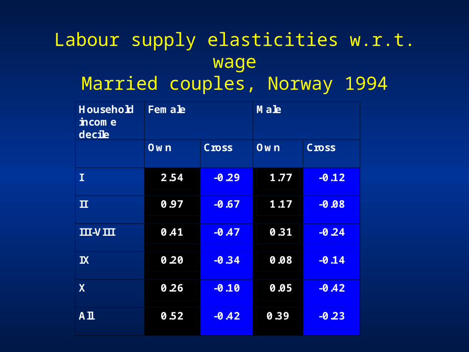
Labour supply elasticities w.r.t. wageMarried couples, Norway 1994

Household income decile

Female Male

Own Cross Own Cross

I 2.54 -0.29 1.77 -0.12

II 0.97 -0.67 1.17 -0.08

III-VIII 0.41 -0.47 0.31 -0.24

IX 0.20 -0.34 0.08 -0.14

X 0.26 -0.10 0.05 -0.42

All 0.52 -0.42 0.39 -0.23

Labour supply elasticities w.r.t. wageMarried couples, Italy 1993

Household income decile

Female Male

Own Cross Own Cross

I 4.44 0.82 0.32 0.06

II 2.31 -0.15 0.17 0.00

III-VIII 0.73 -0.24 0.10 -0.04

IX 0.20 -0.20 0.08 -0.03

X 0.13 -0.17 0.06 -0.02

All 0.66 -0.20 0.12 -0.02

A simulation of some reform proposals in Italy

Two (old) ideas for reforming the tax-transfer system:

• Improving EFFICIENCY by flattening the marginal tax rates

• Improving EQUALITY by introducing a universal transfer or a minimum guaranteed income

Gross income and net income under alternative tax systems

Actual

Gross income

Net income

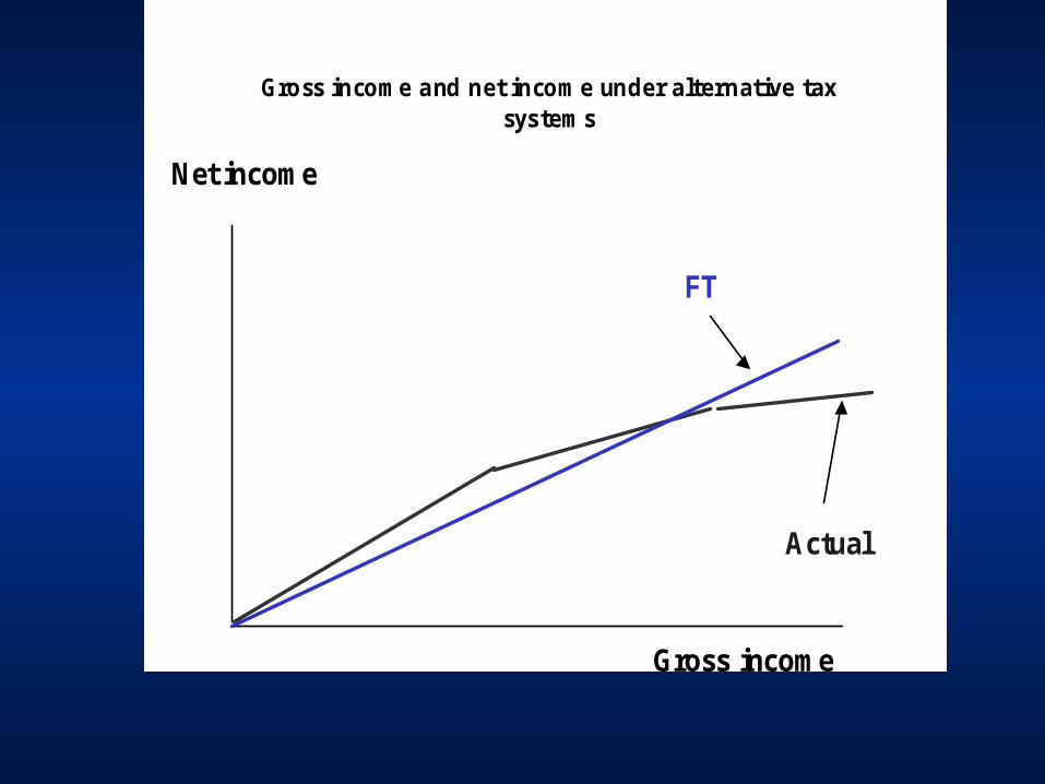
Gross income and net income under alternative taxsystems

Actual

FT

Gross income

Net income

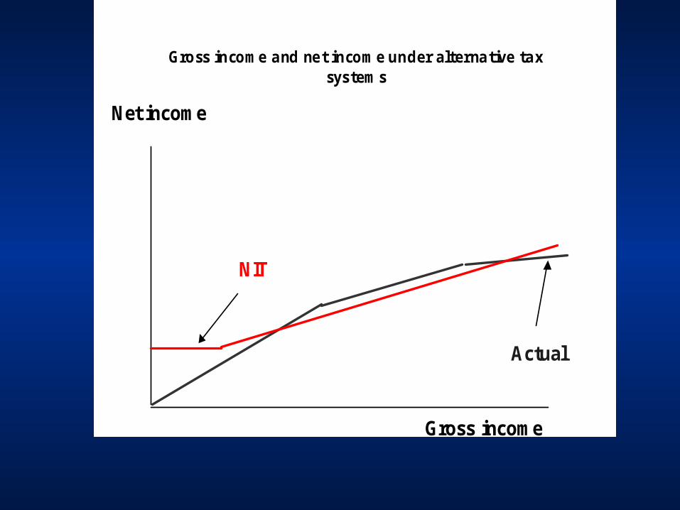
Gross income and net income under alternative taxsystems

Actual

NIT

Gross income

Net income

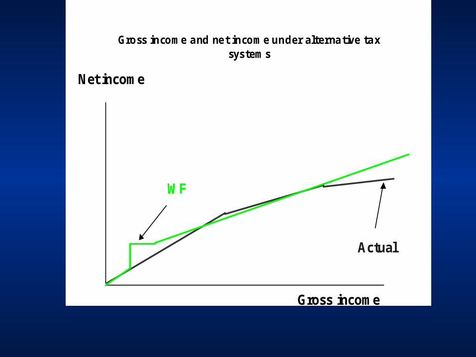
Gross income and net income under alternative taxsystems

Actual

WF

Gross income

Net income

Percentage of “welfare-winners” under alternative tax reforms

49

50

51

52

53

54

55

56

% 51,8 55 55,6

FT NIT WF

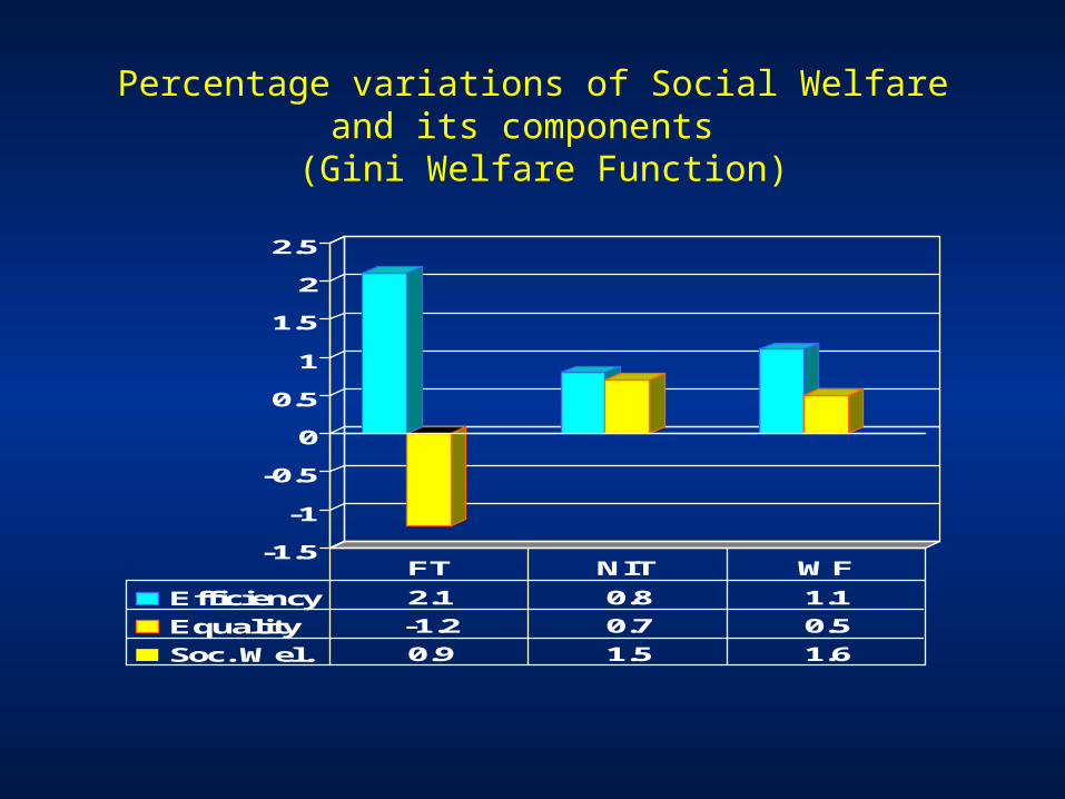
Percentage variations of Social Welfare and its components

(Gini Welfare Function)

-1.5

-1

-0.5

0

0.5

1

1.5

2

2.5

Efficiency 2.1 0.8 1.1

Equality -1.2 0.7 0.5

Soc. Wel. 0.9 1.5 1.6

FT NIT WF

Conclusions

• All the reforms are efficient

• FT is disequalising, but NIT and WF are equalising

• There is scope for designing tax systems that produce bigger “cakes” and more equal “slices” too.

• Of course there might be even better reforms. In what follows we look for optimal reforms …

Optimal taxationAn exercise for Norway

• We use the model to identify optimal tax- transfer rules

• “Optimal” means maximizing a Social Welfare Function

The model

max U(C, h, )s.t.

C=f(wh, I)

(h, w, ) Bwhere:U( ) = utility functionf( ) = tax-transfer ruleC = net incomeh = labour supplyw = wage rate I = exogenous income = other job characteristicsB = opportunity set

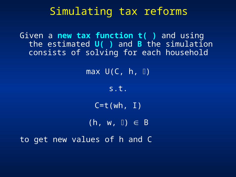
Simulating tax reforms

Given a new tax function t( ) and using the estimated U( ) and B the simulation consists of solving for each household

max U(C, h, )

s.t.

C=t(wh, I)

(h, w, ) B

to get new values of h and C

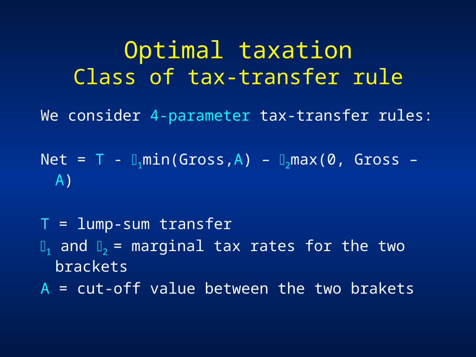
Optimal taxationClass of tax-transfer rule

We consider 4-parameter tax-transfer rules:

Net = T - 1min(Gross,A) – 2max(0, Gross – A)

T = lump-sum transfer1 and 2 = marginal tax rates for the two

bracketsA = cut-off value between the two brakets

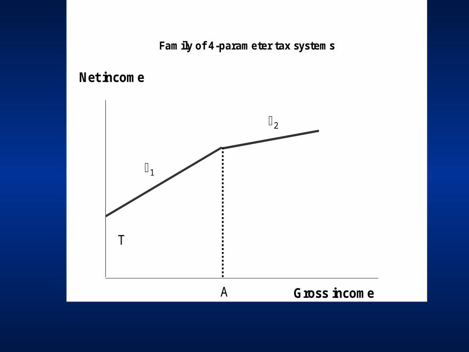
Family of 4-parameter tax systems

Gross income

Net income

T

A

1

2

Optimal taxation: Social Welfare

Function

The Social welfare function is defined as the average individual welfare () times (1 – Inequality Index)

There are many type according to how we define the Inequality Index:

  

  

 Bonferroni: 1

1 1W F (t) log tdt (1 C )

Gini: 12W 2 F (t)(1 t)dt (1 G)

1 233 32W F (t)(1 t )dt (1 C )

Utilitarian: 1W F (t)

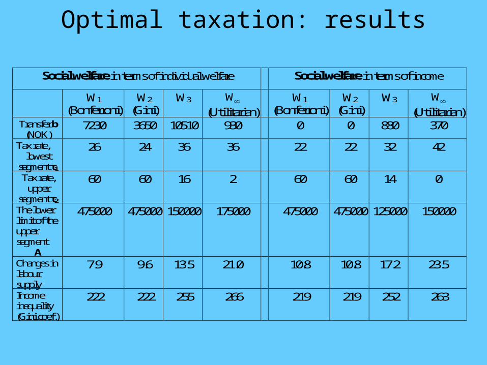
Optimal taxation: results

Social welfare in terms of individual welfare

Social welfare in terms of income

W1

(Bonferroni) W2

(Gini) W3 W

(Utilitarian)

W1

(Bonferroni) W2

(Gini) W3 W

(Utilitarian) Transfer b

(NOK) 7230 3650 10510 930 0 0 880 370

Tax rate, lowest

segment τ1

26 24 36 36 22 22 32 42

Tax rate, upper

segment τ2

60 60 16 2 60 60 14 0

The lower limit of the upper segment

A

475000 475000 150000 175000 475000 475000 125000 150000

Changes in labour supply

7.9 9.6 13.5 21.0 10.8 10.8 17.2 23.5

Income inequality (Gini coef.)

.222 .222 .255 .266 .219 .219 .252 .263

Out-of-sample prediction (Norway)

• In 2001 we are able to observe the effects of a reform of the tax rule actually implemented

• We use the model estimated on 1994 data to simulate the effects of the reform

• We then compare the model predictions to the observed effects…

Out-of-sample prediction

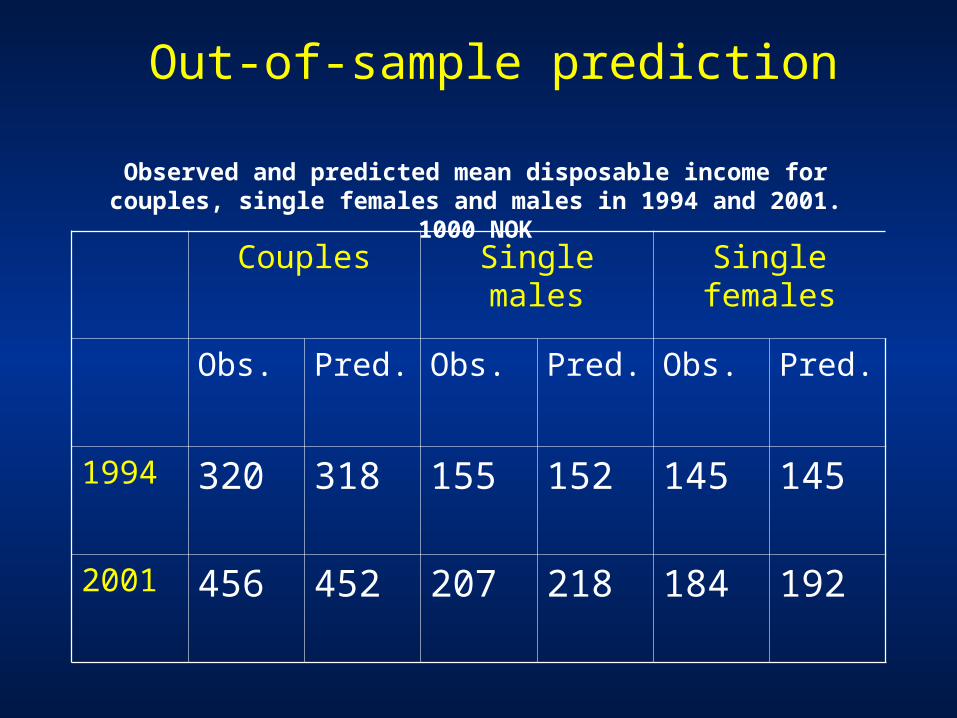
Observed and predicted mean disposable income for couples, single females and males in 1994 and 2001.

1000 NOKCouples Single males Single

females

Obs. Pred. Obs. Pred. Obs. Pred.

1994 320 318 155 152 145 145

2001 456 452 207 218 184 192

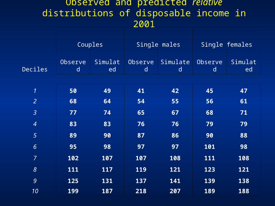
Observed and predicted relative distributions of disposable income in 2001

Couples Single males Single females

DecilesObserve

dSimulate

dObserve

dSimulate

dObserve

dSimulate

d

1 50 49 41 42 45 47

2 68 64 54 55 56 61

3 77 74 65 67 68 71

4 83 83 76 76 79 79

5 89 90 87 86 90 88

6 95 98 97 97 101 98

7 102 107 107 108 111 108

8 111 117 119 121 123 121

9 125 131 137 141 139 138

10 199 187 218 207 189 188

Integrating the Micro- and the CGE- model

CGE model

Microeconometric model

Wage Cash transfersCapital income

Labour supply

Integrating the Micro- and the CGE- model

Simulation at 2050 of a flat tax that supports fiscal equilibrium

Flat Tax

1995 2050

Exogenous

(i.e. without the

Micro model)

24.0

32.0

Labour

Supply Endogenous

(i.e. with the

Micro model)

18.3

22.9