A Microeconometric Test of the Theory of Exhaustible Resources*

Janie M. Chermak Robert H. Patrick Department of Economics Faculty of Management University of New Mexico Rutgers University Albuquerque, NM 87131 Newark, NJ 07102 jchermak@unm.edu rpatrick@andromeda.rutgers.edu

Revised June1999

Abstract

This paper generalizes extant developments of the economic theory of exhaustible resource production, derives and extends a Halvorsen and Smith (1991) type test of the theory, and applies the test to a sample of natural gas resources. To facilitate our empirical test, we extend the model developed in Chermak and Patrick (1995) to explicitly account for the fact that the extracted resource (gross product) must be processed to obtain the final (saleable) product. Duality theory is used to derive econometric models with which the theory is statistically tested, using panel data from 29 natural gas wells. Shadow prices of the resource stock through time, which are generally unobservable but necessary for the test, are estimated via the indirect cost function. Contrary to the extant literature, we find, inter alia, (i) that, at any point in time, ceteris paribus, the in situ resource price (a) decreases with gross production and (b) increases with final production, and (ii) we cannot reject the theory of exhaustible resources, i.e., producer behavior is consistent with the theory. (JEL Q00, L71) 1.0 Introduction

In 1914, Gray argued that modification of Ricardo's 19th century classical notion of rent

is required to accurately account for the exhaustibility of natural resources. Gray, focusing on

the theory of the mine as the appropriate level of aggregation for the analysis, hypothesized that

a price-taking profit maximizing firm, facing u-shaped costs,

* We would like to thank H. Stuart Burness, James Crafton, Robert Halvorsen, Kent Perry; participants at seminars at the American Economic Association Meetings, the European Association of Environmental and Resource Economists Meetings, and Rutgers University; and anonymous referees of this journal for constructive comments on previous versions of this paper; a number of natural gas producing firms for providing data; and the Gas Research Institute for partial financial support. The usual caveat applies.

2

would adjust mine production so that the difference between price and marginal costs of

production would increase at the rate of interest.1 Seventeen years later, Hotelling (1931),

inter alia, formalized this rule at the level of the mine, the firm, and the industry. This research

received little attention until the second half of the twentieth century when concerns of resource

scarcity resulted in a renewed interest in the economics of exhaustible resources. A substantive

body of literature extending and empirically testing the theory has emerged.2 However, lack of

data has generally hampered empirical tests of the theory at all but highly aggregated levels.

Little empirical indication of support for the theory of exhaustible resources has been found,

leaving the question of the theory's usefulness in describing and predicting the behavior of

exhaustible resource producers unresolved.

Existing tests of the theory have, for the most part, used annual data aggregated across

industries (Halvorsen and Smith 1991, Slade 1982, Smith 1979), or monthly industry level data

(Heal and Barrow 1980).3 However, Blackorby and Schworm (1982) demonstrate that

aggregating heterogeneous deposits of a natural resource can result in an aggregate

characterization of technology that doesn’t represent the resource deposits or actual production

technologies. Tests that do not allow for optimal production from the perspective of each

individual deposit have little hope of yielding optimal aggregate production levels. As such, the

focus of this paper is on whether the actual production of individual resource deposits is

consistent with the theory of exhaustible resources. The ultimate question addressed here is the

1 Cairns (1994) proposes this be called the "Gray r-per-cent rule." 2 For a review of the literature, including extensions to the original model, see, for example, Sweeney (1993). Withagen (1998) discusses empirical tests of the theory. 3 Farrow (1985), Slade and Thille (1997), and Stollery (1983) are exceptions, they test the theory using data for a single mine or firm. However, no strong support for the theory is found, as is discussed in more detail below.

3

empirical relevance of a model that is widely used as a positive description of the behavior of

exhaustible resource producers.

This paper develops a test of the theory of exhaustible resources at the level of individual

natural resource deposits. Chermak and Patrick (1995) generalize the economic theory of

exhaustible resource production to (a) allow decreasing marginal production costs, (b) consider

physical bounds on periodic production, and (c) account for interdependency (feedback) between

the stock of the resource, the periodic production bounds, and the chosen production path. In

this paper we extend this model to explicitly recognize that the firm not only extracts the (gross)

resource but also at least partially processes it to arrive at a final product to market. These

generalizations are empirically relevant for the natural gas resources we analyze.4 Duality theory is

used to provide the econometric model with which the theory is statistically tested. The data set,

comprised of 29 wells from five natural gas producing firms, is unique and of sufficient detail to

allow rigorous testing of the theory. Shadow prices of the resource stock through time are

necessary for the test but are not directly observable. Duality theory is used to develop

observable measures of these shadow prices and test the exhaustible resource theory under

alternative specifications of the indirect final cost function, as well as the gross cost function. We

find that the in situ price of the resource decreases with gross (unprocessed) production at any

point in time, and increases with final production at any point in time. Our tests do not reject the

economic theory of exhaustible resources. That is, our estimated final and gross cost functions

indicate that the natural gas resources included in our data were produced in a manner that is

consistent with exhaustible resource theory.

4

The format of the paper is as follows. The next section reviews extant empirical tests of

the exhaustible resource theory, followed by a discussion of the appropriate level of aggregation at

which to test. Our generalized model of exhaustible resource production is presented in Section

4. The econometric model, based on this theory, as well as the specific test of the theory we

employ are presented in Section 5. Data and econometric results are provided in Section 6. A

summary and our conclusions are in Section 7.

2.0 Previous Tests of Exhaustible Resource Theory

The implications of increased natural resource scarcity and its effects on economic

growth have been discussed since at least the 19th century (Ricardo 1817, Gray 1914,

Hotelling 1931). However, the theory was not empirically tested until the second half of the

20th century. Extant empirical tests of the theory have been categorized by Slade and Thille

(1997) into three groups; 1) price behavior, 2) shadow price behavior, and 3) the Hotelling-

Valuation Principle.

The earliest tests were price behavior tests and focused primarily on estimating price

trends as indicators of scarcity. That is, increasing prices indicate increasing scarcity. Barnett

and Morse (1963) plotted annual (1870-1957) industry-level unit prices of extractive products

for five group aggregates (all extractive, minerals, agriculture, forestry, and fishing). With the

exception of forestry and possibly fishing, they found horizontal price trends for the groups.

Smith (1979), in an econometric study of four natural resource aggregates, utilized annual data

4 Contrary to conventional natural gas production, the common pool and joint-production (with oil) problems are not relevant here since we analyze data from "tight-sand" natural gas wells [see Hargoort

5

(1900-1973) and found little evidence of upward trends in prices.5 Smith (p. 426) concludes

"... evaluations of resource scarcity

without detailed analysis of the character of the markets for the specific commodities within each

aggregate, as well as the institutional changes during the period, do not seem possible." Slade

(1982) analyzed long run price movements using annual data (1870-1978) aggregated into

major metals and fuels commodities. Estimating a quadratic functional form, she found support

for three distinct price trends; declining, flat, and increasing. Slade hypothesized the trends

come at different points in the life cycle of the exhaustible resource.

The above studies were based on the examination of product prices and did not test the

coherence of market data with exhaustible resource theory. Heal and Barrow (1980) examined

industry level monthly tin, lead, zinc, and copper data (July, 1965 through June, 1977),

modeling metals prices as a function of interest rates and changes in interest rates. Their

hypothesis is that if an exhaustible resource is an asset, whose price appreciation is a factor in

the holding decision, there are potential arbitrage opportunities between resource markets and

other capital asset markets. They found the change in interest rate, rather than the interest rate

itself, was the significant independent variable. These results (based on commodity prices rather

than in situ prices) are, as the authors conclude, "very tentative" and offer that the results

"...suggest that the matter is considerably more complex than simple equilibrium theory would

suggest" (p. 161).

Shadow prices are not directly observable and hence must be estimated. The shadow

price behavior tests can be sub-divided into two types; estimates which include either explicit or

(1988, Chapter 7) for gas reservoir engineering details in this regard], as discussed in more detail below. 5 The groups included total extraction, minerals, agriculture, and forestry.

6

implicit price expectations.6 The former calculates shadow price as the difference between

(expected) price and marginal cost, which requires specification of an explicit expected price

path through time. This literature includes the following research.

Stollery (1983) tests the theory using a time series of in situ prices. Based on an

extension of the Hotelling pure depletion model that includes the effects of depletion, possible

technical change, and exogenous mineral discoveries, he estimates the in situ price of nickel for

the International Nickel Company (INCO) as the difference between marginal revenue and

marginal cost of extraction. A price leadership model, with INCO as the price leader, is the

assumed market structure. A log-linear demand function and a Cobb-Douglas production

function were estimated with annual data from INCO for 1952-1973. Stollery finds the

resource rent for nickel rose over the time period at a rate compatible with a 15% discount rate.

Employing a capital asset pricing model Stollery argues, given market conditions over this time

period, a 15% discount rate is consistent for INCO.

Farrow (1985) tests the exhaustible resource theory using monthly price and cost data

(January, 1975 through December, 1981) on an underground hard rock mine that produced

several metals commodities as joint products. User cost is calculated as the difference between

product price (estimated as a weighted average of the individual metals commodity prices) and

the marginal extraction cost from an estimated translog cost function. Three model variations

are tested; the basic model with a dynamic discount rate, the basic model extended to include

price expectations, and an extension that include an output constraint. At the level of a single

mine, Farrow does not find support for the exhaustible resource theory.

6 Chermak and Patrick (1999) present a unified analysis of extant tests of the theory.

7

Slade and Thille (1997) integrate the Hotelling theory and the capital asset pricing model

(with extensions) and test this model using annual data (from Young 1992) for fourteen

Canadian copper mines, which operated between 1956 and 1982. They estimate user cost as

the difference between price and marginal extraction costs under several alternative restrictions.

They do not reject the basic theory, although the authors point out the parameter estimates on

the Hotelling variables are “vacuous.” Although the traditional Hotelling model coefficients have

the expected signs and the test results fail to reject this modified Hotelling theory, as the authors

note, only the depletion effect is marginally significant. When risk is incorporated via CAPM

and extensions the empirical performance of the theory improves.

The second type of the behavior of shadow price tests employs duality theory, which

results in the shadow price being estimated directly from the indirect cost function. The

advantage of this test type is that price expectations are included implicitly through the actions of

the firm, whereas the first group requires the price path to be explicitly included, which also

does not allow for different expectations across producers.

Halvorsen and Smith (1984, 1991) utilize duality theory to demonstrate that the in situ

price (user cost) of the resource at any time can be observed by differentiating the indirect cost

function with respect to quantity produced. In their 1991 paper, an econometric model is

derived which provides a statistical test of the theory utilizing annual data from the Canadian

metal mining industry (1954-1974) to test the hypothesis that the time path of in situ prices

satisfies the dynamic optimality condition. The optimality condition is tested under various

discount rates, both constant and varying over the time horizon. The null hypothesis is rejected

under all discount rates tested (2-20%). However, as the authors point out (p. 137) "...the data

8

used to estimate the econometric model are at a high level of aggregation, the empirical results

obtained here should be considered as only tentative."

The third class of test, formulated by Miller and Upton (1985a, b), is a variation of

estimating the transition equation, although it does not hold when there are stock effects in the

cost function. The test is based on an alternative implication derived from Hotelling’s analysis.

It is essentially (1985a, p. 24), “... the value of a unit of reserves in the ground is the same as its

current value above ground less the marginal cost of extracting it, regardless of when the

reserves are extracted.” This formulation was, in part, a response to lack of adequate time

series data with which to test the more traditional implications of the theory. They test this

valuation principle by regressing the market value of oil reserves on their estimated Hotelling

values. The market values are based on a firm’s stock prices, while the Hotelling values are

based on well-head prices, extraction costs, and estimated reserves (extracted from Securities

and Exchange Commission data). 7 The (1985a) results are robust under a variety of

specifications, and the empirical test finds support for the principle under the restriction of no

stock effects on costs. The (1985b) results do not explain as much variation as the (1985a)

data. Miller and Upton conjecture (1985b, p. 1015) the difference in results is due to the

different pricing histories from the two periods, coupled with measurement error.

Withagen (1998) reviews the extant empirical literature and finds the empirical tests

have been hampered by data difficulties (both lack and aggregation of), as well as lack of

information concerning price expectations. The appropriate level of aggregation in exhaustible

resource analyses is examined by Blackorby and Schworm, who theoretically explore two

9

aggregation scenarios with firms extracting from (i) separate resource deposits and (ii) a single

resource deposit. They find that an aggregated model may not be able to replicate actual

behavior of industries or economies extracting from heterogeneous deposits with heterogeneous

technologies. Furthermore, if the restrictions implied by such aggregation assumptions are not

checked, the resulting models may be internally inconsistent with the individual technologies.

If aggregation is appropriate, at what level should we aggregate; the firm level or the

industry level? The following section gives a brief overview of natural gas reservoirs and their

affect on the appropriate level of analysis.

3.0 Level of Analysis

As stated above, Blackorby and Schworm find aggregation may not replicate actual

behavior for an industry when firms are producing from heterogeneous deposits with

heterogeneous technologies. Our research focuses on natural gas resources. In order to

determine the level of analysis at which to conduct this research, a brief description of natural

gas reservoirs and how they are produced is important to determine if aggregation is

appropriate, and if so, at what level.

The majority of natural gas reservoir rocks were formed either by (1) deposition of rock

fragments of older rocks, or (2) chemical or organic precipitation. The amount of gas

potentially available for production is a function of the reservoir characteristics, specifically;

porosity, permeability, and water saturation, which measure the total amount of void space in

the rock, the ability of fluids to move through the rock, and the amount of the void space that is

7 The 1985a data coverage is December 1979-August 1981, while the 1985b data coverage is August 1981-December 1983. The authors (1985b, p. 1015) point out that the first data set covers a time period of large

10

water-filled, respectively. These reservoir characteristics are affected not only by the

depositional environment, but also by the post-depositional environment. The spatial

environment can rapidly change and, consequently, not only can porosity, permeability, and

water saturation vary between reservoirs, they can vary within reservoirs. It follows that the

production potential of one well may not be the same as the production potential of another well

in the same field. Aggregating wells within the same field, which have heterogeneous reservoir

characteristics would be the equivalent of aggregating heterogeneous deposits.8

The second consideration in the level of analysis is technology. For natural gas

production, this focuses on (i) how the well is completed, and (ii) how the well is produced. By

completion, we refer to procedures that enhance recovery. The most common being fracturing

which induces manmade conduits (fractures) from the wellbore into the surrounding reservoir to

allow easier gas flow to the wellbore. The technology of hydraulic fracturing has progressed

over the years, as has the understanding of the effect of fracture geometry on production.

Fracturing techniques vary across the wells comprising our data, which implies heterogeneous

technologies across these wells.

Production technology includes not only the physical diameter of the wellbore pipe, but

also the production choice. Natural gas production is normally pressure driven. That is, the

natural pressure within the reservoir is used as the mechanism for pushing the gas to the surface.

variation in oil prices, while the second data set has relatively little price variation. 8 An important consideration in the analysis is that of the common pool. High permeability indicates easy fluid flow, which can result in the common pool problem, that is, production in one sector of the field can drain gas from another sector, adversely affecting reserves. Tight gas reservoirs are defined (legally) as reservoirs with an average reservoir permeability of less than .01 millidarcy, which is very low. As the name might suggest, tight gas reservoirs do not exhibit easy flow of fluids through the formation and interaction between wells is not common. The data used in this research is from tight sand gas reservoirs, and so the common pool problem is not considered in the analysis.

11

The deeper the reservoir, in general, the higher the initial reservoir pressure.9 Low production

quantities, in a given time period, are achieved by using only a small portion of the reservoir

pressure, i.e., restricting production by allowing only a portion of the physically producible gas

to come to surface. All wells are not produced in a similar manner. This brings us to our final

aggregation consideration; the effect of past production on future potential. As a well is

produced, the reservoir pressure declines. Different production paths lead to different pressure

decline profiles, which result in different future potentials. This further complicates the ability to

aggregate.

Given the heterogeneity of wells from the physical, technological, and past production

history aspects, the appropriate level of analysis is at the level of the deposit, which is the

individual well in the case of natural gas from tight sands.

4.0 The Theory of Exhaustible Resources

This section presents the profit-maximizing problem for the price-taking firm producing a

non-renewable resource subject to a capacity constraint on periodic production as well as the

traditional resource stock constraint. Furthermore, we consider the effect of extraction on the

production capacity and stock constraints, common to natural gas production, as well as the fact

that some processing of gross production may be necessary.

Formally, we consider maximum production at t, Q(t) = Q(q) , (where

q = {q( t) : t ∈[0,t)}), as a functional of the function q (t) , the gross production at time t. Each

9 Initial reservoir pressure is a function of, among other things, the depth from surface of the reservoir. The U.S. Energy Information Administration (1990) reports natural gas production depths from less than 3,000 to in excess of 15,000 feet. Average production depths for active wells range from 5,500 feet for pre-1957 vintage wells to 6,600 feet for 1985-1988 vintage wells. Again, heterogeneity among wells is indicated.

12

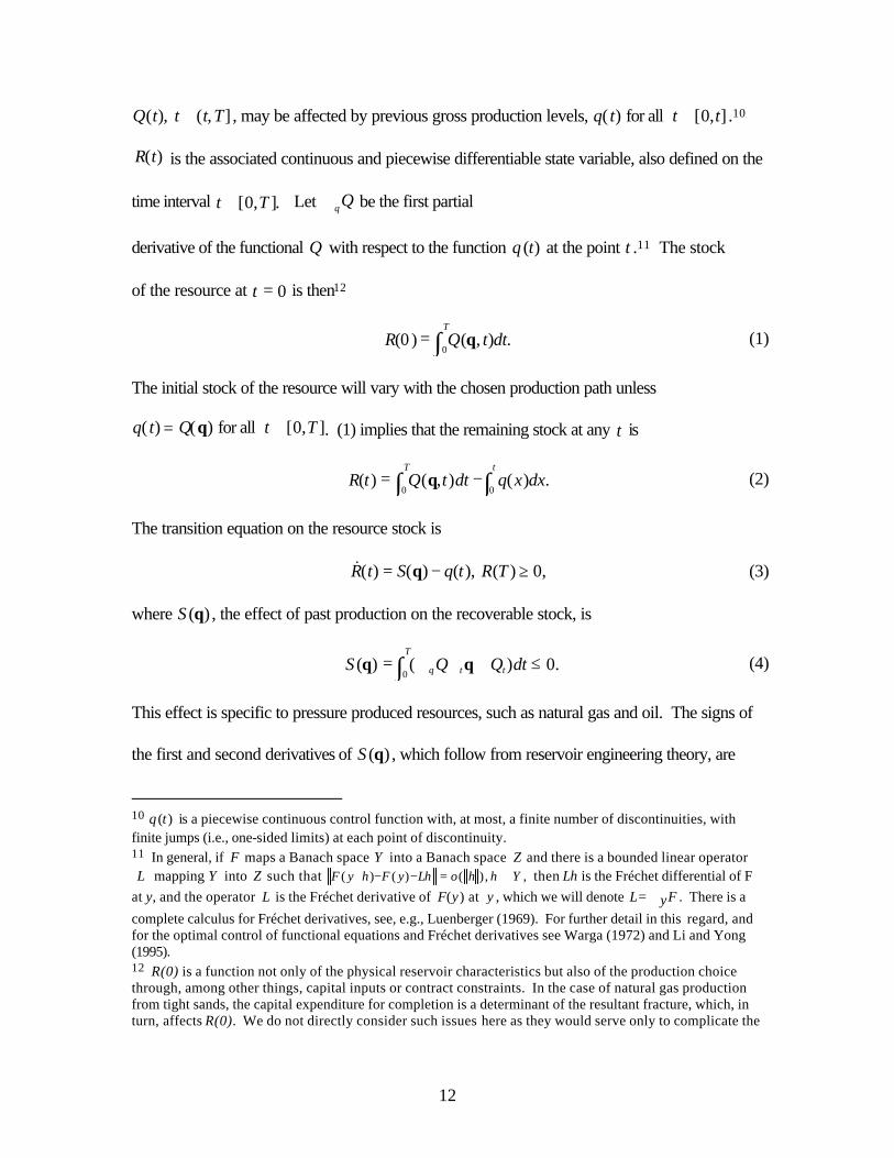
Q(t), t ∈(t,T] , may be affected by previous gross production levels, q( t) for all t ∈[0,t] .10

R(t) is the associated continuous and piecewise differentiable state variable, also defined on the

time interval t ∈[0,T ]. Let ∇qQ be the first partial

derivative of the functional Q with respect to the function q (t) at the point t .11 The stock

of the resource at t = 0 is then12

R(0 ) = Q(q, t)dt.0

T

∫ (1)

The initial stock of the resource will vary with the chosen production path unless

q( t) = Q(q) for all t ∈[0,T ]. (1) implies that the remaining stock at any t is

R(t) = Q(q,t)dt −0

T

∫ q(x)dx.0

t

∫ (2)

The transition equation on the resource stock is

&( ) ( ) ( ), ( ) ,R t S q t R T= − ≥q 0 (3)

where S (q) , the effect of past production on the recoverable stock, is

S (q) = (∇q0

T

∫ Q∇tq + Qt)dt ≤ 0. (4)

This effect is specific to pressure produced resources, such as natural gas and oil. The signs of

the first and second derivatives of S (q) , which follow from reservoir engineering theory, are

10 q (t ) is a piecewise continuous control function with, at most, a finite number of discontinuities, with finite jumps (i.e., one-sided limits) at each point of discontinuity. 11 In general, if F maps a Banach space Y into a Banach space Z and there is a bounded linear operator L mapping Y into Z such that ( ) ( ) ( ), ,F y h F y Lh h h Yο+ − − = ∈ then Lh is the Fréchet differential of F

at y, and the operator L is the Fréchet derivative of F(y) at y , which we will denote L yF= ∇ . There is a

complete calculus for Fréchet derivatives, see, e.g., Luenberger (1969). For further detail in this regard, and for the optimal control of functional equations and Fréchet derivatives see Warga (1972) and Li and Yong (1995). 12 R(0) is a function not only of the physical reservoir characteristics but also of the production choice through, among other things, capital inputs or contract constraints. In the case of natural gas production from tight sands, the capital expenditure for completion is a determinant of the resultant fracture, which, in turn, affects R(0). We do not directly consider such issues here as they would serve only to complicate the

13

nonpositive. S (q) = 0 for non-pressure produced resources, in which case (3) becomes

&( ) ( )R t q t= − , i.e., the transition equation in traditional exhaustible resource models.

Gross production from the well is not necessarily the amount of gas that can be sold by

the firm. The removal of non-hydrocarbon gases from the natural gas and other shrinkage

generally prohibit this.13 Let q( t) = g(Xg ,R,t) represent the gross production function where

{ }( ) : 1,...,gjx t j J= =X are inputs into the gross production process. The final production of

natural gas (i.e., the amount that is input into the pipeline to be transported to purchasers) is given

by z( t) = f (X f ,q, t) , where { }( ) : 1,...,fkx t k K= =X are inputs used to process gross

production to arrive at the final product at each t, z(t). Naturally, final production can be no

greater than gross production, i.e., z ≤≤ q .

The firm's problem is to choose the input production paths, the gross production path, and

the production time horizon to maximize profits, π , of the quasi-fixed resource.14 The firm's

objective is then to choose X f q t t T T, for and ( ) [ , ],∈ 0 to maximize

0

[ ( ) ( ) ( , ( ), ( ) , )] ,T rt f f ge P t z t C q t R t t dtπ −= − ⋅ −∫ W X W (5)

where P(t) is the output price per unit of final production, z(t), { }( ) : 1,...,fkw t k K= =W are

processing input prices, { }( ) : 1,...,ggw t j J= =W are prices of inputs into gross production, and

the gross cost function (the dual to the gross production function) is given by

economics without adding any compensating insight. See Kuller and Cummings (1974) in the case of oil production and Patrick and Chermak (1992) and Chermak and Patrick (1995) in natural gas production. 13 The US Energy Information Administration (Natural Gas Annuals, various years) distinguishes gross withdrawals, defined as full well-stream volume excluding condensate separated at the lease from dry natural gas production defined as gross withdrawals less gas diverted for repressuring, quantities vented or flared, non-hydrocarbon gas removed in the treatment or processing, and extraction losses. 14 Generally, the firm would have a number of wells under its control and, with costs estimated at the well level, would choose the number of wells to produce and simply sum revenues and costs of all wells.

14

C q t R t t q g R tg

X

g g gg

( , ( ), ( ), ) min ( , , ).W W X X≡ = s. t. (5’)

Profits are maximized subject to the resource stock constraint, (3), and bounds on gross

production at any time

0 ≤ q(t) ≤ Q(q) , (6)

where ∇qQ ≤ 0 , which implies, e.g., that increasing q at any t may reduce Q for all future t ,

and ∇qqQ ≥ 0 . The upper bound on periodic production, Q , is a natural physical

constraint, based on current reservoir pressure. Initial reservoir pressure is a function of depth

and formation characteristics. Once extraction begins, the upper bound declines over time due

to declining reservoir pressure. The rate of decline in pressure is affected by past production. In

practice Q and R are incorporated into the economic model through reservoir engineering

theory.15

The Hamiltonian for this problem is

H(t) = e− rt[P(t)z(t) − W f ⋅ X f − C(Wg ,q(t), R(t), t)] + λ[S(q) − q(t)] , (7)

where λ is the multiplier (in situ resource price) on (3), the transition equation of the resource

stock. The generalized Hamiltonian is

L(t) = H(t) + η[Q(q) − q(t)] , (7')

where η is the multiplier on (6), the upper bound production constraint at each t . Necessary

conditions include

− = = −L e CRrt

R&λ , (8)

However, considering the number of wells to produce adds to the notational complexity of the analysis without providing compensating insights or any qualitative differences in the results presented below. 15 See Patrick and Chermak (1992) and Chermak, et al., (1999).

15

{ }

* * * * *

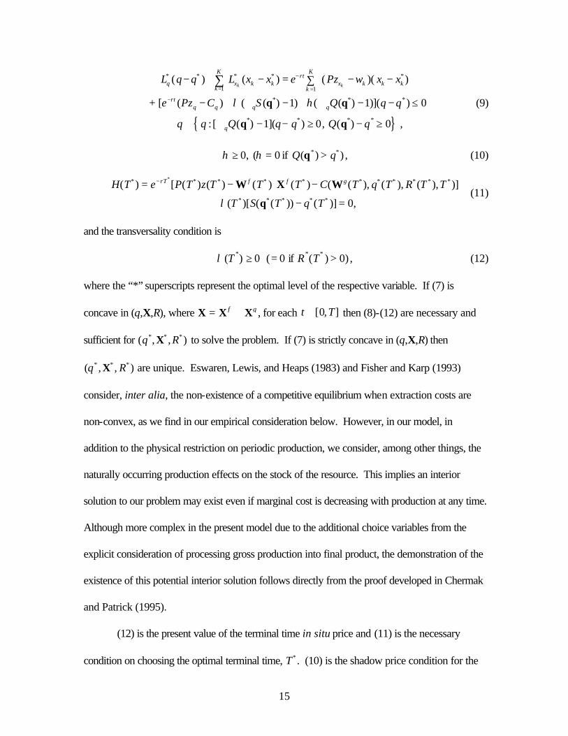
1

* * *

* * * *

1( ) ( ) ( )( )

+ [ ( ) ( ( ) 1) ( ( ) 1)]( ) 0

: [ ( ) 1]( ) 0, ( ) 0 ,

k k

Krt

q x k k x k k kk

rtq q q q

q

K

kL q q L x x e Pz w x x

e Pz C S Q q q

q q Q q q Q q

λ η

−

=

−

=− + − = − −∑

− + ∇ − + ∇ − − ≤

∀ ∈ ∇ − − ≥ − ≥

∑

q q

q q

(9)

η ≥ 0, (η = 0 if Q(q*) > q*) , (10)

H T e P T z T T T C T q T R T T

T S T q T

rT f f g( ) [ ( ) ( ) ( ) ( ) ( ( ), ( ), ( ), )]

( )[ ( ( )) ( )] ,

* * * * * * * * * * *

* * * * *

*

= − ⋅ −

+ − =

− W X W

qλ 0 (11)

and the transversality condition is

λ (T *) ≥ 0 (= 0 if R*(T* ) > 0) , (12)

where the “*” superscripts represent the optimal level of the respective variable. If (7) is

concave in (q,X,R), where X = X f ∪ Xg , for each t ∈[0,T] then (8)-(12) are necessary and

sufficient for (q*,X* ,R*) to solve the problem. If (7) is strictly concave in (q,X,R) then

( , , )* * *q RX are unique. Eswaren, Lewis, and Heaps (1983) and Fisher and Karp (1993)

consider, inter alia, the non-existence of a competitive equilibrium when extraction costs are

non-convex, as we find in our empirical consideration below. However, in our model, in

addition to the physical restriction on periodic production, we consider, among other things, the

naturally occurring production effects on the stock of the resource. This implies an interior

solution to our problem may exist even if marginal cost is decreasing with production at any time.

Although more complex in the present model due to the additional choice variables from the

explicit consideration of processing gross production into final product, the demonstration of the

existence of this potential interior solution follows directly from the proof developed in Chermak

and Patrick (1995).

(12) is the present value of the terminal time in situ price and (11) is the necessary

condition on choosing the optimal terminal time, T* . (10) is the shadow price condition for the

16

physical capacity constraint. (9) is the optimality condition on gross production and other inputs

into final production, q * and X f *, for each t ∈[0,T *] . λ( )t ≥ 0 for all t T∈[ , ]*0 is implied by

(8) and (12), i.e., λ( )*T ≥ 0 by (12) and (8) implies the present value user cost is declining over

t, &λ = <−e CrtR 0, since CR < 0 (cost increases as the stock of the resource is depleted). (8) is

the dynamic optimality condition for the exhaustible resource, which is used in the econometric

tests developed in the next section.

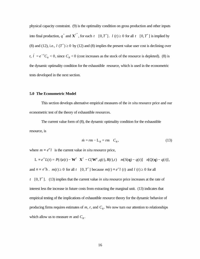
5.0 The Econometric Model

This section develops alternative empirical measures of the in situ resource price and our

econometric test of the theory of exhaustible resources.

The current value form of (8), the dynamic optimality condition for the exhaustible

resource, is

&m rm rm CR R= − = +L , (13)

where m ≡ ertλ is the current value in situ resource price,

L ≡ ertL(t) = P( t)z(t) − W f ⋅ X f − C(Wg ,q(t), R(t),t) + m[S(q) − q(t)] + n[Q(q) − q(t)] ,

and n ≡ ertη . m t( ) ≥ 0 for all t T∈[ , ]*0 because m t e trt( ) ( )≡ λ and λ( )t ≥ 0 for all

t T∈[ , ]*0 . (13) implies that the current value in situ resource price increases at the rate of

interest less the increase in future costs from extracting the marginal unit. (13) indicates that

empirical testing of the implications of exhaustible resource theory for the dynamic behavior of

producing firms requires estimates of m, r, and CR . We now turn our attention to relationships

which allow us to measure m and CR .

17

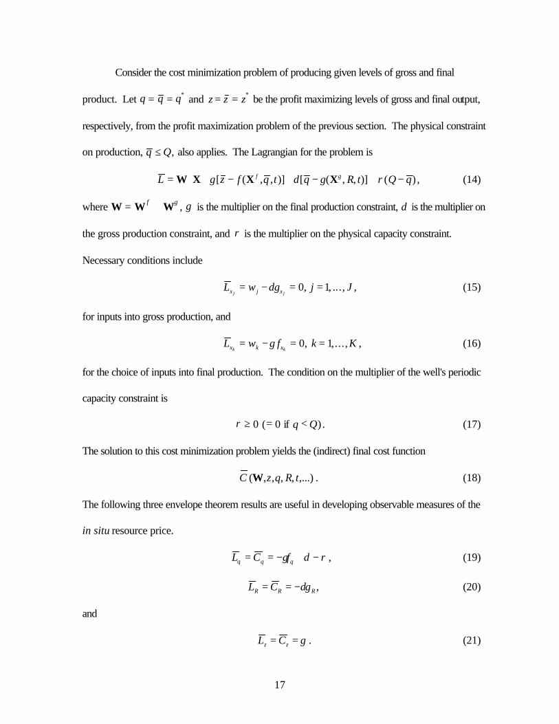
Consider the cost minimization problem of producing given levels of gross and final

product. Let q = q = q* and z = z = z* be the profit maximizing levels of gross and final output,

respectively, from the profit maximization problem of the previous section. The physical constraint

on production, q Q≤ , also applies. The Lagrangian for the problem is

L z f q t q g R t Q qf g= ⋅ + − + − + −W X X Xγ δ ρ[ ( , , )] [ ( , , )] ( ) , (14)

where W = W f ∪ Wg , γ is the multiplier on the final production constraint, δ is the multiplier on

the gross production constraint, and ρ is the multiplier on the physical capacity constraint.

Necessary conditions include

L w g j Jx j xj j= − =δ 0 1, = , ..., , (15)

for inputs into gross production, and

L w f k Kx k xk k= − =γ = ,...0 1, , , (16)

for the choice of inputs into final production. The condition on the multiplier of the well's periodic

capacity constraint is

ρ ≥ 0 (= 0 if q < Q) . (17)

The solution to this cost minimization problem yields the (indirect) final cost function

C (W,z,q, R, t,...) . (18)

The following three envelope theorem results are useful in developing observable measures of the

in situ resource price.

L C fq q q= = − + −γ δ ρ , (19)

L C gR R R= = −δ , (20)

and

L Cz z= = γ . (21)

18

Now consider the firm's problem of minimizing the cost of producing z, treating q as an

endogenous input into the production of z. The inputs, X, are now chosen to minimize costs,

defined as W X X⋅ + mg R tg( , , ), where m is the (unobserved) shadow price of the resource in

situ, subject to the constraints on final and periodic production, z = z = z* and 0 ≤ ≤q Q . The

Lagrangian for the cost minimization problem when gross production, q, is endogenous is then

L = W ⋅ X + mg(X g, R,t) + ˜ γ [z − f (X f ,g(Xg , R, t), t)]+ ˜ ρ [Q − g(Xg ,R,t)], (22)

where ˜ γ is the multiplier on the final production constraint and ˜ ρ is the multiplier on the physical

capacity constraint. Necessary conditions include

L w m f g j Jx j g xj j= + − − =[ ~ ~] ,γ ρ 0 =1, ..., , (23)

for the optimal choice of inputs into gross production;

L w f k Kx k xk k= − =~ , ,γ = ,...0 1 , (24)

for the optimal choice of inputs (other than q) into final production and

~ ( )ρ ≥ = <0 0 if q Q . (25)

Envelope theorem results include

L C m f gR R q R= = − −( ~ ~)γ ρ , (26)

The optimal X for this problem is identical to that from the previous problem since q = q = q*

and z = z = z* . (16) and (24) then imply that γ γ= ~ . (15), (17), (23), and (25) then lead to

ρ ρ= ~ and δ γ ρ= − + +m fq~ ~ . Substituting these expressions into (19) leads to the result stated

in Lemma 1.

Lemma 1. The current value in situ resource price is equal to the negative of the marginal final

cost of gross production, i.e., m Cq= − .

19

Halvorsen and Smith (1984, 1991), as discussed in Section 2, derived this result in their

exhaustible resource model. Lemma 1 and m ≥ 0 imply that Cq ≤ 0, i.e., the marginal final cost

of gross production is nonpositive. The intuition here is that additional q, all else held constant,

reduces the marginal cost of producing a given level of z. Lemma 1 also implies that the current

value in situ resource price can be observed by differentiating the estimated indirect final cost

function with respect to gross production, q. Analogous to the demonstration of Lemma 1,

substituting δ γ ρ= − + +m fq~ ~ into (26) and using (20), it follows that L R = LR and hence

C R = CR . Thus, by estimating the indirect final cost function, (18), and differentiating with

respect to q and R we can observe m and CR , which are required in testing (13), the dynamic

optimality condition.

To obtain another observable measure of the in situ resource price, as well as gain further

insight into Lemma 1, consider the profit maximization model in Section 4 and recall that the

above cost minimization problems are evaluated at the profit maximizing levels of z and q. For

simplicity in allowing us to focus on measuring the in situ price, we write the model in current

value form, take the feedback effect as insignificant, and assume an interior solution.16 The

current value Hamiltonian for the profit maximization problem is then

H t P t z t C q t R t t mq tf f g( ) ( ) ( ) ( , ( ), ( ), ) ( )= − ⋅ − −W X W . (27)

Necessary conditions include

− = = +H m rm CR R& , (28)

16 The relationship between gross and final production is more complicated than modeled here, and requires the incorporation of reservoir engineering theory, as well as the gas properties to discern it to a greater degree than in this consideration. Although we have made significant progress in such modeling (see Chermak, et al., 1999), this is beyond the scope of this paper and is left for future research. Nonetheless, our relatively simple exhaustible resource models tested here are consistent with producer behavior.

20

H Pf C mq q q= − − = 0, (29)

H Pf wx x kk k= − = 0, (30)

H T P T z T T T

C T q T R T T m T q T

f f

g

( ) ( ) ( ) ( ) ( )

( ( ), ( ), ( ), ) ( ) ( ) ,

* * * * * *

* * * * * * * * *

= − ⋅

− − =

W X

W 0 (31)

and the transversality condition is

m T R T( ) ( ( ) )* * *≥ = >0 0 0 if , (32)

As above, since λ( )t ≥ 0 and m t e trt( ) ( )≡ λ , m ≥ 0 . Substituting (29) into (30) we

have

( / )w f f C mk q x qk= + . (30’)

(16) and (21) into (30’) lead to m f C C f Cq q z q q= − = −γ . We summarize this result in the

following Lemma.

Lemma 2. The current value in situ resource price is equal to the value (in terms of the

marginal final cost of z) of the marginal product of q less the marginal gross cost, i.e.,

m C f Cz q q= − ≥ 0.

The gross cost minimization problem, (5’), in Section 4 implies Cq ≥ 0. Given production occurs,

the marginal product of q, fq , is positive. We expect the marginal final cost (the marginal cost of

producing the final product) to be positive, Cz > 0 . The value of the marginal product of q must

then be greater than the marginal gross cost of q, C f Cz q q> , for the inequality in Lemma 2 to hold.

Further development of the implications of Lemma 2, and other results which follow, are

developed in Chermak and Patrick (1999).

21

The differential equation (13) can be solved to provide a more convenient form for

testing the dynamic optimality condition since our estimated indirect gross and final cost function

is (statistically) autonomous. (13), multiplied by e−rt , can be rewritten as

d (e− rtm) / dt = e− rtCR ,

which, after integrating and rearranging, leads to17

0

( ) (0) ,trt rt rx

Rm t e m e e C dx−− = ∫

or, in discrete time,

m t e m r Crt t x

x

t

R( ) ( ) ( )− = + −

=∑0 1

0

.

Substituting m = −C q and CR = C R , from our results above, yields

00

(1 )t

rt t xq t q R

x

e C C r C−=

=

− = + ∑ , (13')

which is the form of the dynamic optimality condition we use to restrict the parameters of the

indirect final cost function, (18), in econometrically testing the exhaustible resource theory.

Specifically, we want to test the null hypothesis, that (13') is satisfied by our parameter estimates

for (18), against the alternative hypothesis, that (13') is not satisfied by our parameter estimates

for (18). This hypothesis is tested with a Hausman (1978) specification test by estimating (18)

with and without the restriction implied by (13'). We perform an analogous, although more

complicated, test on the gross cost function, (5’), using Lemma 2.

17Rather than using the initial time we could use the traditional terminal time development of the constant of integration. Using the terminal time condition, H(T)=0, it is also easy to see that m(t)≥0. That is, since

( ) [ ( ) ( ) ( )] ( ) 0 and 0R

f fP T T T C T q T C− + ≥ <W X , we have

( )

0( ) [ ( ) ( ) ( )] ( )( ) (0) 0rt rt r t T rt

R R

t Trx rx

t

f fP T T T C T q Tm t e C dx e m e e C dxe e−− − − + + = − ≥= ∫ ∫W X.

See Chermak and Patrick (1995) for further detail.

22

Hausman's test requires that we have (i) an asymptotically efficient estimator under the

null hypothesis which is not consistent under the alternative hypothesis and (ii) another estimator

that is asymptotically less efficient than the first under the null hypothesis and consistent under the

alternative. Estimation of equation (18) and (5’) provide consistent estimates of the parameters

of the indirect final and gross cost functions, respectively, regardless of whether the time path of

in situ prices conforms to (13'). Estimation of the constrained equations, (18) with (13') and

(5’) with (13’), provide consistent and asymptotically efficient estimates of the parameters of the

indirect final and gross cost functions under the null hypothesis in each case, but inconsistent

estimates under the alternative. Denote the first estimator by the vector ˆ β and the second by the

vector ~β . Let ˆ V be a consistent estimator of asymptotic variance-covariance matrix of ( $ ~

)β β− .

The Hausman statistic is then

( $ ~) $ ( $ ~

)β β β β− ′ −−V 1 , (22)

which, under the null hypothesis, is asymptotically χ2 distributed with degrees of freedom equal to

the dimension of the vector β .

6.0 Data, Empirical Specification and Results

The test of the theory of exhaustible resources is performed on our econometrically

estimated indirect cost function developed above. The data set is comprised of 443

observations from 29 tight sand gas wells. Seventeen of the wells are located in Wyoming and

twelve in Texas. The data is monthly, over the time period of 1987 through 1991.18

18 Monthly observations are used since they are an accepted norm in the industry. A possible concern would be if there is a detectable change on a monthly basis. Certainly from the production perspective, monthly changes are discernible. The Energy Information Administration (1990) shows monthly production declines between 4% and 8% a month during the first year of production, resulting in 50% drop in

23

The wells in our data set vary in age from the initial month of production through the 29th

year of production. The wells also vary in, among other things, physical characteristics such as

(i) gross pay thickness (21 to 133 feet), (ii) production depths (5,400 to 10,400 feet), and (iii)

reservoir characteristics of porosity, permeability, and water saturation. The data, provided by

five firms, include (1) recoverable reserves, (2) gross monthly production, (3) monthly extraction

and production costs, (4) the producing formation, (5) location, and (6) the beginning month of

production for each well, as well as the physical characteristics for each well. In addition to this

data, described in detail in Patrick and Chermak (1992) and Chermak and Patrick (1995), we

also use final production data from ten of these wells.

We specify the indirect final cost function in the form of a Generalized Cobb-Douglas,

where monthly production costs, C , are hypothesized to be a function of gross production, q,

final production, z, remaining reserves, R, and production month, pm. We use a fixed effects

model which stratifies the panel data by firm and year. Our general (unrestricted) specification

of the indirect final cost function is

(FC ) U1

ln ln ln ln ln ,C D D q z R pm ei=

N

i i y yy

Y

q z R pm

i

= + + + + + +∑ ∑=

α α β β β β2

i=1,...,N firms, y=1,...,Y years, and ewt = the customary error term, a random number with zero

mean. Since there is a strong relationship between z and q, this specification of the final cost

function may be problematic in terms of separating the effects of z and q on final costs.

Therefore, in addition to the unrestricted form above (FCU), we estimate two restricted forms of

production quantities from the beginning to the ending of the first year of production. During later production periods, the declines are lower. This results in a steeply downward sloping production path early in a well’s life, followed by a fairly flat production path during later stages. Of course, the actual path and percentage changes during a given month depend on the specific well and the production plan followed by the producer.

24

the final cost function. Given the theoretical developments above, we estimate a function (FCR)

that restricts the parameter estimates on final and gross production to be of opposite sign but

equal in absolute value (i.e., β βz q= − ). We also estimate an average final cost function

(FC ) A1

ln ln ln ln lnC z D D q R pm ei=

N

i i y yy

Y

q R pm

i

− = + + + + +∑ ∑=

α α β β β2

which imposes a parameter estimate of positive one on z, i.e., constant marginal cost of final

production. Halvorsen and Smith (1991) estimate an analogous average cost function in their

test of the theory. 19 Finally, we estimate an indirect gross cost function (GC), which is

specified analogous to the general form of the final cost function with the restriction z=0, i.e.,

(GC) 1

ln ln ln lnC D D q R pm ei=

N

i i y yy

Y

q R pm

i

= + + + + +∑ ∑=

α α β β β2

.

The three final cost models (FCU, FCR, and FCA) are employed as our empirical

specifications of (18), while the gross cost function, GC, is employed as our empirical

specification of (5’). Differentiating the resulting final cost specification (FCU, FCR, or zFCA)

with respect to q and R, applying Lemma 1, and substituting into (13') provides the parametric

form of the dynamic optimality condition for the final cost models. Testing GC requires an

analogous process, using Lemma 2, to derive the implied constraints on the parameters of the

gross cost function.

Unfortunately, final production data are not available for all our observations on gross

production and the other available data. However, as discussed in the theoretical development

above, final production is a function of, and can be no greater than, gross production. To avoid

discarding important information contained in the incomplete data and improve efficiency of our

25

estimates, missing z observations were estimated from the available data (Griliches 1986,

Greene 1997) according to $ $ ,$ $

z q pmzzq zp= α β β subject to z ≤≤ q , where parameters are defined

analogous to the above. Production month is included to allow for changes in the composition

of the natural gas over the life of the

well. Changes in gas composition may, for instance, result in the increased production of non-

hydrocarbon gases over time. Our econometrically estimated final production function is then

ln . . ln . ln ,z q pm= − + −3116 10349 0228

(.0365) (.0039) (.004)

where standard errors are in parentheses.20 For comparison sake, the average value on gross

production is 19,057 mcf per month, relative to a mean of 18,557 for final production, with a

standard deviations of 19,308 and 19,164, respectively.

The parameter estimates for the three specifications of the final cost function and the

gross cost specification, are presented in Table 1.21 The first four parameter estimates are

associated with gross production, final production, remaining reserves, and the production

month, respectively. The remaining nine parameter estimates are fixed effects terms for firms

one through five and years 1988 through 1991, respectively.

19 Contrary to this average cost specification, Halvorsen and Smith’s (1991) specified average cost per unit value of output rather than the average cost per unit of output. 20 The regression was estimated using full feasible generalized least squares (FGLS, see, e.g., Greene 1997). First order autocorrelation was indicated by the Durbin Watson statistic; an iterative Prais -Winsten algorithm was used in the correction. Results from both Ramsey RESET and White tests indicate the null hypothesis of homoskedasticity cannot be rejected. 127 observations were available to estimate this equation, which is also characterized by a ρ =.41235 (with a standard error of .08116) and a log-likelihood of 281.24. 21 As above, FGLS was employed for all regressions. Durbin Watson statistics indicated first order autocorrelation in each of the four models. An iterative Prais -Winsten algorithm was used in the corrections. Ramsey RESET and White tests indicate the null hypothesis of homoskedasticity cannot be rejected.

26

As expected, parameter estimates in all four models indicate costs increase as the

resource is exhausted. The parameter estimate on R, the stock of the resource remaining at time

t, is significant at the 5% level in FCU and the 10% level in FCR, FCA, and GC. Production

month is not significant in FCU, but is significant at the 5% level in FCR; the 1% level in FCA,

and the 10% level in GC. In all specifications, the individual firm intercepts are positive and

significant at the 5% level. The parameter estimates on the years are significant in 1989 and

1990 (at 10% and 5%, respectively) in FCR and FCA, and in 1990 (at 10%) in both FCU and

GC.

The estimated parameters on z and q are significant at least at the 5% level in all four

regression equations. According to the theory developed above, the final cost function should

be characterized by Cz ≥ 0and Cq ≤ 0, while for the gross cost function, Cq ≥ 0. This implies

the estimated parameters should be β z ≥ 0 and β q ≤ 0 for final costs, and, for gross costs,

β q ≥ 0 . With the exception of FCU, the signs on the estimated parameters are as we would

expect from the theory. Contrary to the theory, FCU indicates the parameter on z is significantly

negative, i.e., final costs are inversely related to final production.22 However, final production is

naturally restricted to be no greater than gross production and there exists a strong relationship

between gross and final production, although this does not prohibit obtaining significant

parameter estimates on these variables. The parameter estimates β z and β q in FCU have a

relatively large and negative covariance. We therefore examine final cost functional forms which

22 Although there is some intuitive appeal to these results. Holding all else constant, increased final production means an increased ratio of final to gross product. Higher ratios of final to gross product translate into less non-hydrocarbon gases and water, which must be separated and disposed of during processing, which results in lower processing costs.

27

do not explicitly include separate independent variables for z and q, i.e., FCR and FCA, as

specified above.

Next we statistically compare the three forms of the final cost function estimated. If we

restrict β z == 1 and divide FCU by z, we have FCA, which is analogous the functional

specification assumed in Halvorsen and Smith (1991). Restricting FCU by β βz q= − , leads to

FCR. To compare the three forms of the final cost function we use a Wald statistic to test the

following restrictions on the parameters of FCU;

FCA: H0 : βz == 1 versus H1 : β z ≠≠ 1

and

FCR: H Hz q z q0 1: : versus β β β β= − ≠ − .

The resulting Wald values are 9.383 and .000049, respectively. The Wald value for FCA is

greater than the critical χ 2 value, indicating we reject the null hypotheses (.05 level of

significance) of the average final cost model. The Wald value for FCR is less than the critical χ 2

value, indicating we do not reject the null hypotheses (.01 level of significance) that β q and β z

are of opposite signs and equal in absolute value. Thus we have statistical support for the FCR

specification of the final cost function.

Contrary to the findings of others, our gross and final cost function estimates imply that

marginal costs of gross and final production are decreasing with increases in q and z,

respectively. That is, for GC, Cq > 0 and Cqq < 0 , and, for FCR, Cz > 0 and Czz < 0 . How

the in situ resource price varies with changes in q and z is also of interest. Again, our results

are contrary to extant results. To see this, differentiate FCR with respect to q, which leads to

Cq < 0 and Cqq > 0 . Since m Cq= − (Lemma 1), m Cq qq= − < 0, which implies, ceteris

28

paribus, that the in situ resource price decreases with gross production at any point in time.

Considering the relationship between final production and the in situ resource price in an

analogous fashion, we have Cqz < 0 which leads to m Cz qz= − > 0 . This implies, ceteris

paribus, that the in situ resource price increases with final production at any point in time.

The dynamic optimality condition is tested under all three specifications of the final cost

function using Lemma 1, the specified gross cost function using Lemma 2, and a range of discount

rates for all models. If natural gas wells are produced in a manner consistent with the theory then

the production decision is effectively made taking into account the opportunity cost of current

production (the in situ resource price or user cost) and the path is economically optimal

according to our theory. Table 2 presents the Hausman statistics for the four models at various

discount rates. As indicated, the theory is not rejected at the 0.05 significance level in any of our

estimated models or for any of the discount rates tested.23 That is, our estimated final and gross

cost functions indicate that the natural gas resources included in our data were produced in a

manner that is consistent with Hotelling’s theory.

Finally, we estimate the user cost (in situ resource price) from FCR using Lemma 1.

User cost across all wells ranges from $0.000004 (per mcf) to $3.18, with a mean value of

$0.0766, a median of $0.0233, and a standard deviation of $0.21. These values, however, are

aggregated across the entire data set, which has a tendency to mask variations across wells.

The importance of using the appropriate level of analysis is highlighted by the variation of user

cost across wells. As can be seen from Table 3, there are significant differences across wells.

23 As is common in the literature (e.g., Halvorsen and Smith 1991), we present the tests for discount rates of no greater than 20%. However, we performed the test for larger discount rates and reached exactly the same conclusions.

29

These differences across the wells may be attributed to differences in reservoir properties, age

of the well, ownership, and location, among other things.24

While Table 3 presents the summary statistics, it does not adequately represent the user

cost path through time for any of the wells. Figure 1 presents the daily production and user cost

paths for Well 12b.25 All else equal, we expect user cost values to monotonically decline over

time, as theoretically demonstrated in Section 4. However, all else is not held constant in Figure

1. Overlaying the daily production path helps to explain the deviations: when gross production

is relatively low, user cost is high; conversely, when gross production is relatively high, user cost

is relatively low. This is the expected relationship, as shown above, given our result of declining

marginal costs of gross production.

7.0 Summary and Conclusions

This paper presents a test of the theory of exhaustible resources at the level of individual

natural resource deposits. We generalize extant developments of the economic theory of

exhaustible resource production, derive and extend a Halvorsen and Smith (1991) type test of

this theory, and apply the test to a sample of natural gas resources. To facilitate our empirical

test, the model developed in Chermak and Patrick (1995) is extended to explicitly account for

the fact that the resource is not only extracted but also processed. Duality theory is then used to

derive the econometric model with which the theory is statistically tested, employing panel data

from 29 natural gas wells. Shadow prices of the resource stock through time that are generally

24 See Patrick and Chermak (1992) and Chermak and Patrick (1995) for additional detail on differences across the wells comprising this data set. 25 Well 12 was chosen for illustration purposes since it has one of the longest production histories of any of the wells in the data set. The other wells comprising the data set present analogous results.

30

unobservable but necessary for the test, are estimated via the indirect final cost function.

Contrary to the extant literature, our test, carried out at the level of the individual resource,

indicates that the theory can, indeed, be useful in describing the behavior of an individual

producer.

The theory and the test as derived above assume, among other things, that all decisions

are made under complete certainty.27 A natural extension to this research is to explicitly

incorporate risk into the analysis. However, given the results we obtain, it is likely that

generalizing the model to explicitly consider uncertainty would only serve to reinforce our results

concerning the predictive ability of the theory for the natural gas resources considered in this

paper.

27 Gilbert (1979), Pindyck (1980), Dasgupta and Stiglitz (1981), and Deshmukh and Pliska (1985) generalize the traditional Hotelling model to formally consider various aspects of uncertainty.

31

References

Barnett, H.J. and C. Morse (1963). Scarcity and Growth: The Economics of Natural

Resource Availability, Baltimore, MD, Johns Hopkins University Press. Blackorby, Charles and William Schworm (1982). "Rationalizing the Use of Aggregates in

Natural Resource Economics." In W. Eichhorn, et al., eds. Economic Theory of Natural Resources, Wursburg, Germany, Physica-Verlag.

Cairns, Robert D. (1994). "On Gray's Rule and the Stylized Facts of Non-Renewable

Resources." Journal of Economic Issues 18(3):777-798. Chermak, J.M. and R.H. Patrick (1995). "A Well-Based Cost Function and the Economics of

Exhaustible Resources: The Case of Natural Gas." Journal of Environmental Economics and Management 28(2):174-189.

Chermak, J.M. and R.H. Patrick (1999). "Reconciling Tests of the Theory of Exhaustible

Resources." Mimeo. Chermak, J.M., J. Crafton, S. Norquist, and R.H. Patrick (1999). "A Hybrid Economic-

Engineering Model for Optimal Natural Gas Production," Energy Economics 21(1):67-94.

Dasgupta, Partha and Joseph Stiglitz (1981). "Resource Depletion Under Technological Uncertainty." Econometrica XLIX: 85-104.

Deshmukh, Suhakar D. and Stanley R. Pliska (1985). "A Martingale Characterization of the

Price of a Nonrenewable Resource with Decisions Involving Uncertainty." Journal of Economic Theory 35: 322-42.

Energy Information Administration (1990) Natural Gas Production Responses to a

Changing Market Environment 1978-1988, Washington, D.C., U.S. Government Printing Office.

Eswaran, M., T.R. Lewis, and T. Heaps (1983). "On the Nonexistence of Market Equilibria in

Exhaustible Resource Markets with Decreasing Costs." Journal of Political Economy 91:154-167.

Farrow, Scott (1985). "Testing the Efficiency of Extraction from a Stock Resource." Journal of

Political Economy 93(3):452-487. Fisher, Anthony C., and Larry S. Karp (1993). "Nonconvexity, Efficiency and Equilibrium in

Exhaustible Resource Depletion." Environmental and Resource Economics 3:97-106.

32

Gilbert, Richard (1979). "Optimal Depletion of an Uncertain Stock." Review of Economic

Studies 46: 47-57. Gray, Lewis C. (1914). "Rent Under the Assumption of Exhaustibility." Quarterly Journal of

Economics XXVI:497-519. Greene, William H. (1997). Econometric Analysis Third Edition, New Jersey, Prentice Hall. Griliches, Zvi (1986). “Economic Data Issues.” In Zvi Griliches and Michael D. Intriligator,

Eds., Handbook of Econometrics Vol. 3, Amsterdam, North-Holland. Halvorsen, Robert, and Tim R. Smith (1991). "A Test of the Theory of Exhaustible Resources."

Quarterly Journal of Economics CVI(2):123-140. Halvorsen, Robert, and Tim R. Smith (1984). "On Measuring Natural Resource Scarcity."

Journal of Political Economy 92:954-64. Hargoort, Jacques (1988). Fundamentals of Gas Reservoir Engineering, New York,

Elsevier Publishers. Hartwick, John M. (1989). Non-renewable Resources, Extraction Programs, and Markets,

Chur, Switzerland, Harwood Academic Publishers. Hausman, Jerry A. (1978). "Specification Tests in Econometrics." Econometrica 46:161-81. Heal, Geoffrey, and Michael Barrow (1980). "The Relationship Between Interest Rates and

Metal Price Movements." Review of Economic Studies 47:161-81. Hotelling, Harold (1931). "The Economics of Exhaustible Resources." Journal of Political

Economy 39(2):137-175. Kuller, Robert G., and Ronald G. Cummings (1974). "An Economic Model of Production and

Investment for Petroleum Reservoirs." American Economic Review 64(1):66-79. Li, Xunjing, and Jiongmin Yong (1995). Optimal Control Theory for Infinite Dimensional

Systems, Birkhäuser, Boston. Luenberger, David G. (1969). Optimization by Vector Space Methods, Wiley, New York. Miller, Merton H., and Charles W. Upton (1985a). "A Test of the Hotelling Valuation

Principle." Journal of Political Economy 93(1):1-25. Miller, Merton H., and Charles W. Upton (1985b). "The Pricing of Oil and Gas: Some Further

Results." Journal of Finance 40:1009-1018.

33

Patrick, R.H., and J.M. Chermak (1992). The Economics of Technology Research and

Development: Recovery of Natural Gas from Tight Sands. Gas Research Institute Report No. GRI-92/0267, Washington, D.C.: National Technical Information Services.

Pindyck, Robert S. (1980). "Uncertainty and Exhaustible Resource Markets." Journal of

Political Economy 88:1203-25. Ricardo, David (1817). The Principles of Political Economy and Taxation., London,

Everyman's Library, 1987 reprint. Seierstad, Atle, and Knut Sydsæter (1987). Optimal Control Theory with Economic

Applications, Amsterdam, North-Holland. Slade, Margaret E. (1982). "Trends in Natural Resource Commodity Prices: An Analysis of the

Time Domain." Journal of Environmental Economics and Management 9:122-37. Slade, Margaret E., and Henry Thille (1997). "Hotelling Confronts CAPM: A Test of the Theory

of Exhaustible Resources." Canadian Journal of Economics 30:685-708. Smith, V. Kerry (1981). "The Empirical Relevance of Hotelling's Model for Natural

Resources." Resources and Energy 3:105-117. Smith, V. Kerry (1979). "Natural Resource Scarcity: A Statistical Analysis." Review of

Economic and Statistics 61:423-27. Stollery, Kenneth R. (1983). "Mineral Depletion with Cost as the Extraction Limit: A Model

Applied to the Behavior of Prices in the Nickel Industry," Journal of Environmental Economics and Management, 10:193-208.

Sweeney, James (1993). "Economic Theory of Depletable Resources: An Introduction." In A.

Kneese and J. Sweeney, Eds., Handbook of Natural Resource and Energy Economics Vol. 3, Amsterdam, North-Holland.

Veatch, R.W., et al. (1989). "An Overview of Hydraulic Fracture." In E. Gidley, et al., Eds.,

SPE Monograph: Recent Advances in Hydraulic Fracturing, Richardson, TX, Society of Petroleum Engineers.

Warga, J. (1972). Optimal Control of Differential and Functional Equations, New York,

Academic Press. Withagen, Cees (1998). "Untested Hypotheses in Non-renewable Resource Economics."

Environmental and Resource Economics 11(4):623-34.

34

Young, D. (1992). "Cost Specification and Firm Behavior in a Hotelling Model of Resource Extraction." Canadian Journal of Economics 25:41-59.

Table 1: Regression Results FCU FCR FCA GC

Parameter Estimate s.e. Estimate s.e. Estimate s.e. Estimate s.e. $q 3.117b 1.340 -0.863a 0.032 -0.996a 0.011 0.038a 0.011 $z -2.976b 1.296 0.863a 0.032 - - - - $R -0.057b 0.028 -0.048c 0.029 -0.052c 0.028 -0.053c 0.029 $p -0.014 0.032 0.056b 0.023 0.059a 0.022 0.041c 0.022

"Firm 1 6.084a 0.642 7.351a 0.508 7.383a 0.497 7.057a 0.494 "Firm 2 5.719a 0.615 6.926a 0.488 6.957a 0.478 6.647a 0.474 "Firm 3 7.539a 0.634 8.823a 0.493 8.842a 0.485 8.525a 0.482 "Firm 4 7.923a 0.613 9.222a 0.465 9.241a 0.455 8.91a 0.452 "Firm 5 7.113a 0.632 8.849a 0.480 8.449a 0.472 8.114a 0.468 "1988 -0.106 0.221 -0.157 0.224 -0.161 0.223 -0.147 0.222 "1989 -0.318 0.228 -0.383c 0.231 -0.382c 0.230 -0.366 0.229 "1990 -0.377c 0.226 -0.449b 0.229 -0.451b 0.228 -0.432c 0.227 "1991 -0.234 0.236 -0.326 0.237 -0.329 0.237 -0.305 0.236

ρ 0.72a 0.033 0.731a 0.032 0.728a 0.033 0.726a 0.033 Log-L -57.88 -62.61 -62.64 -60.55

s.e.≡standard error; level of significance: a=0.01, b=0.05, and c=0.10

Table 2: Dynamic Optimality Test Results*

Discount Rate Hausman Statistics FCU FCR FCA GC

0.02 8.028 3.828 6.622 0.52098 0.05 7.678 1.799 6.365 0.52097 0.10 7.279 0.993 6.051 0.52094 0.12 7.184 1.781 5.961 0.52093 0.14 7.093 2.359 5.889 0.52093 0.15 7.047 2.571 5.859 0.52099 0.16 6.994 2.734 5.832 0.52092 0.17 6.993 2.849 5.809 0.52091 0.18 6.970 2.922 5.789 0.52099 0.19 6.916 2.957 5.771 0.52090 0.20 6.920 2.958 5.757 0.52099

*Distributed χ 2 with 4 degrees of freedom for the FCU function and 3 degrees of freedom for the FCR, FCA, and GC models. The critical value, at the 0.05 level of significance, of the test statistic is 9.488 for 4 degrees of freedom and 7.815 for three degrees of freedom.

37 37

TABLE 3: In Situ Resource Price Summary Statistics ($/mcf)

WELL MEAN MEDIAN S.D. MIN MAX 1 0.045403 0.016853 0.109975 0.011564 0.539374 2 0.143274 0.135364 0.028912 0.107679 0.232192 3 0.210166 0.198573 0.053081 0.162773 0.452002 4 0.523268 0.431558 0.320705 0.289788 1.406445 5 0.049406 0.048963 0.005694 0.040987 0.063665 6 0.030388 0.013397 0.055413 0.010515 0.231854 7 0.015759 0.016946 0.005264 0.005758 0.024646 8 0.209025 0.019042 0.767903 0.010064 3.188560 9 0.021090 0.020658 0.002332 0.018651 0.024872 10 0.244624 0.041013 0.572365 0.037445 1.661108 11 0.015812 0.015415 0.001772 0.012801 0.018782

12(a)* 0.000017 0.000014 0.000009 0.000010 0.000041 12(b)* 0.102597 0.092587 0.028073 0.082101 0.202578 12(all)* 0.061565 0.087874 0.055272 0.000010 0.202578

13 0.000031 0.000028 0.000006 0.000022 0.000042 14 0.070902 0.056291 0.044138 0.036664 0.189397 15 0.058237 0.044176 0.034011 0.027809 0.145935 16 0.038588 0.029117 0.022569 0.020923 0.090375 17 0.041794 0.027793 0.041223 0.015691 0.165709 18 0.064496 0.053762 0.031250 0.032286 0.142233 19 0.022708 0.019412 0.008851 0.014364 0.044792 20 0.027950 0.024072 0.012030 0.013910 0.052832 21 0.018774 0.014783 0.012510 0.007138 0.047392 22 0.069305 0.063948 0.035380 0.024208 0.158955 23 0.056153 0.054375 0.028449 0.022671 0.119454 24 0.000004 0.000004 0.000001 0.000004 0.000006 25 0.000018 0.000018 0.000006 0.000011 0.000034 26 0.000024 0.000024 0.000003 0.000021 0.000029 27 0.000033 0.000033 0.000010 0.000018 0.000049 28 0.000004 0.000004 0.000001 0.000004 0.000005 29 0.000164 0.000168 0.000019 0.000138 0.000203

ALL 0.076574 0.023262 0.210104 0.000004 3.188560 *Well 12 changed ownership at the end of the 16th month of production.

38 38

Figure 1: In Situ Resource Price and Gross Production Paths for Well 12b

User Cost (m ) and Gross Production (q )

0

0.05

0.1

0.15

0.2

0.251 4 7 10 13 16 19 22 25

Month

Use

r Cos

t ($/

mcf

)

00.20.40.60.811.2

Gro

ss P

rodu

ctio

n

(mm

cfd)

User Cost

Gross Production