a port-hamiltonian model of liquid sloshing in moving

A port-Hamiltonian model of liquid sloshing in moving containers andapplication to a fluid-structure systemI

Flavio Luiz Cardoso-Ribeiro, Denis Matignon, Valerie Pommier-Budinger1

Institut Superieur de l’Aeronautique et de l’Espace (ISAE-SUPAERO)Universite de Toulouse, 31055 Toulouse Cedex 4, France

Abstract

This work is motivated by an aeronautical issue: the fuel sloshing in the tank coupled with very flexible wings.Vibrations due to these coupled phenomena can lead to problems like reduced passenger comfort and maneuverability,and even unstable behavior. Port-Hamiltonian systems (pHs) provide a unified framework for the description of multi-domain, complex physical systems and a modular approach for the interconnection of subsystems. In this work, pHsmodels are proposed for the equations of liquid sloshing in moving containers and for the structural equations ofbeams with piezoelectric actuators. The interconnection ports are used to couple the sloshing dynamics in the movingtank to the motion the beam. This coupling leads to an infinite-dimensional model of the system in the pHs form.A finite-dimensional approximation is obtained by using a geometric pseudo-spectral method that preserves the pHsstructure at the discrete level. Experimental tests on a structure made of a beam and a tank were carried out to validatethe finite-dimensional model of liquid sloshing in moving containers. Finally, the pHs model proves useful to designan active control law for the reduction of sloshing phenomena.

Keywords: port-Hamiltonian systems, shallow-water sloshing, moving container, dynamic coupling, interconnectionof systems, active control

1. Introduction

The fluid motion in moving containers is a subject of concern in several engineering disciplines. In the aeronauticaldomain, the fuel inside tanks can modify the flight dynamics of airplanes [1], potentially leading to fatal accidents.Two practical examples of coupling between the airplane rigid body dynamics and fuel sloshing are given in [2]:during the Korean War, several crashes of the Lockheed F-80C jet fighter were caused by an unstable coupling between5

the short period mode and the fluid; the Dutch roll mode of Douglas A4D Skyhawk presented undamped oscillationsdue to a coupling with fuel motion. Other applications where this phenomenon plays an important role include rocketsand satellites with liquid propellant [3, 4], tank trucks and aircraft with aerial dispersant systems [5].

Besides, the use of new light-weight materials and the optimization of the airplane structure usually leads toincreased structural flexibility. For this reason, the sloshing dynamics inside the tank can couple with the wing10

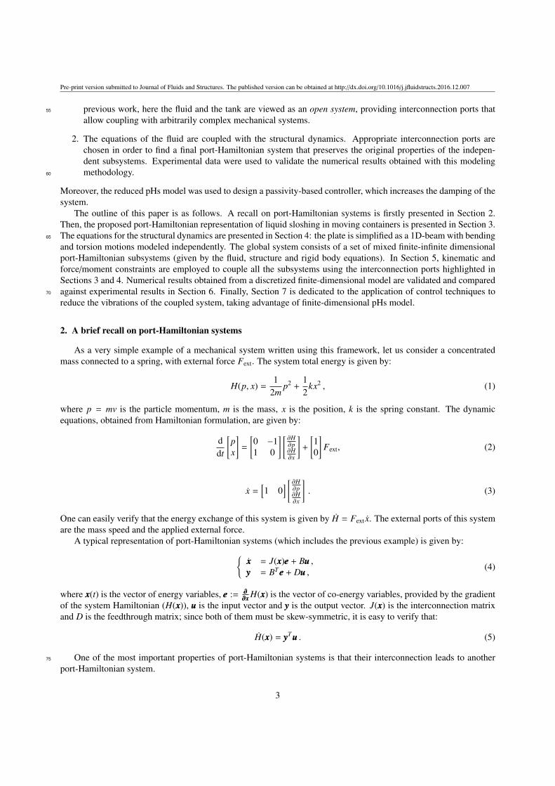
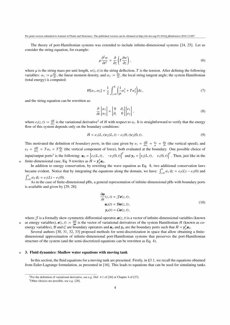
structural dynamics, possibly leading to reduced maneuverability, reduced comfort and even changes in the stabilitybehavior [6]. At ISAE, we have an experimental device to study this coupled problem. The device consists of analuminum plate clamped at one end with a water tank near the free tip. The fluid dynamics and structural dynamicshave similar natural vibration frequencies, leading to strong dynamic coupling between them. The device is depictedin Figs. 1 and 2. Two piezoelectric patches are attached near the clamped end of the beam to reduce the vibrations15

actively. Two accelerometers near the free end are used to measure the motion of the structure. This device waspreviously modeled and controlled in [7, 8, 9]. The main goal of this work is to propose a modular mathematicalmodel of this system that can be used for simulation and control design.

IThis work was partially supported by ANR-project HAMECMOPSYS ANR-11-BS03-0002.1The author F. L. Cardoso-Ribeiro is on leave from the Instituto Tecnologico de Aeronautica with financial support from CNPq - Brazil.

Preprint submitted to Journal of Fluids and Structures. The published version can be obtained at http://dx.doi.org/10.1016/j.jfluidstructs.2016.12.007

Pre-print version submitted to Journal of Fluids and Structures. The published version can be obtained at http://dx.doi.org/10.1016/j.jfluidstructs.2016.12.007

Piezo actuators

TankBeam

AccelerometersFigure 1: Experimental setup schematic representation

Figure 2: Experimental device

The use of port-based modeling [10] is a recent trend in systems analysis and control. This formulation, proposedby Henry Paynter [11], allows describing complex systems as composed of several simpler subsystems which interact20

through a pair of variables, whose product equals power. The energy exchange between each subsystem is viewed asa common language for describing the interaction of systems of different domains (thermal, mechanical, electrical,etc.).

The port-Hamiltonian formulation [12] combines the port-based modeling with Hamiltonian systems theory. Thisapproach was initially designed for studying finite-dimensional complex systems (like networks of electric circuits)25

[13, 14, 15]. Among its properties, this methodology allows coupling multi-domain systems in a physically consistentway, i.e., using energy flow, so that interconnections are power-conserving.

Shallow Water Equations (SWE, also known as Saint-Venant equations) are probably the simplest infinite-dimen-sional mathematical representation for a fluid with free-surface. Nevertheless, these equations are still studied forthe modeling and control of sloshing in moving tanks. Ref. [16] proposed new equations, where the tank horizontal30

position and rotation angle are the control inputs of the system. Refs. [17] and [18] studied the coupling betweenSaint-Venant equations with a horizontally moving vehicle. In this case, a Hamiltonian formulation is proposed,allowing the use of a symplectic integration scheme. Refs. [19], [20] generalized the sloshing equations in movingtanks for 2D and 3D motions for prescribed tank motions. Ref. [21] studied the problem of stabilization of a tankwith fluid using Lyapunov functions.35

The SWE were also recently studied in the port-Hamiltonian framework but with a different goal: modeling andcontrolling the flow on open channel irrigation systems [22, 23]. In this case, there is neither rotation nor translationof the channels.

In the context of dynamic modeling and numerical simulation, the methodology proposed in this paper transformsthe classical Lagrangian formulation of the dynamics to a port-Hamiltonian formulation, expressed as a system of40

conservation laws. This approach departs from [18], where the Hamiltonian system is defined with respect to asymplectic form, whereas the Hamiltonian formulation presented in this paper is defined with respect to a Hamiltoniandifferential operator.

In the context of systems theory, the port-Hamiltonian model of the fluid proposed here enables a modular repre-sentation of the liquid sloshing that can be interconnected to complex technological structures. The proposed model45

for liquid sloshing can be used for the case of moving containers.Finally, in the context of fluid control, we assume indirect actuation fixed on the flexible structure (using piezo-

electric actuators) instead of direct actuation of the speed or acceleration of the tank (as [16] and [21]). Furthermore,the port-Hamiltonian approach provides a natural framework for passivity-based control design, since the systemHamiltonian provides a storage function and can be used as a candidate Lyapunov function. This method differs from50

previous work on the same experimental device that used H∞ control techniques for finding controllers that attenuatethe fluid-structure coupled vibrations [7, 9].

The main contributions of this paper are the following:

1. A port-Hamiltonian representation of the liquid sloshing in moving containers is proposed. Differently of

2


previous work, here the fluid and the tank are viewed as an open system, providing interconnection ports that55

allow coupling with arbitrarily complex mechanical systems.

2. The equations of the fluid are coupled with the structural dynamics. Appropriate interconnection ports arechosen in order to find a final port-Hamiltonian system that preserves the original properties of the indepen-dent subsystems. Experimental data were used to validate the numerical results obtained with this modelingmethodology.60

Moreover, the reduced pHs model was used to design a passivity-based controller, which increases the damping of thesystem.

The outline of this paper is as follows. A recall on port-Hamiltonian systems is firstly presented in Section 2.Then, the proposed port-Hamiltonian representation of liquid sloshing in moving containers is presented in Section 3.The equations for the structural dynamics are presented in Section 4: the plate is simplified as a 1D-beam with bending65

and torsion motions modeled independently. The global system consists of a set of mixed finite-infinite dimensionalport-Hamiltonian subsystems (given by the fluid, structure and rigid body equations). In Section 5, kinematic andforce/moment constraints are employed to couple all the subsystems using the interconnection ports highlighted inSections 3 and 4. Numerical results obtained from a discretized finite-dimensional model are validated and comparedagainst experimental results in Section 6. Finally, Section 7 is dedicated to the application of control techniques to70

reduce the vibrations of the coupled system, taking advantage of finite-dimensional pHs model.

2. A brief recall on port-Hamiltonian systems

As a very simple example of a mechanical system written using this framework, let us consider a concentratedmass connected to a spring, with external force Fext. The system total energy is given by:

H(p, x) =1

2mp2 +

12

kx2 , (1)

where p = mv is the particle momentum, m is the mass, x is the position, k is the spring constant. The dynamicequations, obtained from Hamiltonian formulation, are given by:

ddt

[px

]=

[0 −11 0

] [ ∂H∂p∂H∂x

]+

[10

]Fext, (2)

x =[1 0

] [ ∂H∂p∂H∂x

]. (3)

One can easily verify that the energy exchange of this system is given by H = Fext x. The external ports of this systemare the mass speed and the applied external force.

A typical representation of port-Hamiltonian systems (which includes the previous example) is given by:xxx = J(xxx)eee + Buuu ,yyy = BTeee + Duuu , (4)

where xxx(t) is the vector of energy variables, eee := ∂∂∂∂x∂x∂x H(xxx) is the vector of co-energy variables, provided by the gradient

of the system Hamiltonian (H(xxx)), uuu is the input vector and yyy is the output vector. J(xxx) is the interconnection matrixand D is the feedthrough matrix; since both of them must be skew-symmetric, it is easy to verify that:

H(xxx) = yyyTuuu . (5)

One of the most important properties of port-Hamiltonian systems is that their interconnection leads to another75

port-Hamiltonian system.

3


The theory of port-Hamiltonian systems was extended to include infinite-dimensional systems [24, 25]. Let usconsider the string equation, for example:

µ∂2w∂t2 =

∂

∂z

(T∂w∂z

), (6)

where µ is the string mass per unit length, w(z, t) is the string deflection, T is the tension. After defining the followingvariables: α1 := µ ∂w

∂t , the linear moment density, and α2 := ∂w∂z , the local string tangent angle; the system Hamiltonian

(total energy) is computed:

H[α1, α2] =12

∫ L

z=0

(1µα2

1 + Tα22

)dz , (7)

and the string equation can be rewritten as:

∂

∂t

[α1α2

]=

[0 ∂z

∂z 0

] [e1e2

], (8)

where ei(z, t) := δHδαi

is the variational derivative2 of H with respect to αi. It is straightforward to verify that the energyflow of this system depends only on the boundary conditions:

H = e1(L, t)e2(L, t) − e1(0, t)e2(0, t) . (9)

This motivated the definition of boundary ports, in this case given by e1 = δHδα1

= α1µ

= ∂w∂t (the vertical speed), and

e2 = δHδα2

= Tα2 = T ∂w∂z (the vertical component of force), both evaluated at the boundary. One possible choice of

input/output ports3 is the following: uuu∂ =[e1(L, t) , −e2(0, t)

]Tand yyy∂ =

[e2(L, t) , e1(0, t)

]T. Then, just like in the

finite-dimensional case, Eq. 9 rewrites as H = yyyT∂uuu∂.80

In addition to energy conservation, by rewriting the wave equation as Eq. 8, two additional conservation lawsbecame evident. Notice that by integrating the equations along the domain, we have:

∫ Lz=0 α1 dz = e2(L) − e2(0) and∫ L

z=0 α2 dz = e1(L) − e1(0).As in the case of finite-dimensional pHs, a general representation of infinite-dimensional pHs with boundary ports

is available and given by [29, 28]:

∂ααα

∂t(z, t) = Jeee(z, t) ,

uuu∂(t) = Bααα(z, t) ,yyy∂(t) = Cααα(z, t) ,

(10)

whereJ is a formally skew-symmetric differential operator,ααα(z, t) is a vector of infinite-dimensional variables (knownas energy variables), eee(z, t) := δH

δαααis the vector of variational derivatives of the system Hamiltonian H (known as co-85

energy variables), B and C are boundary operators and uuu∂ and yyy∂ are the boundary ports such that H = yyyT∂uuu∂.

Several authors [30, 31, 32, 33] proposed methods for semi-discretization in space that allow obtaining a finite-dimensional approximation of infinite-dimensional port-Hamiltonian systems that preserves the port-Hamiltonianstructure of the system (and the semi-discretized equations can be rewritten as Eq. 4).

3. Fluid dynamics: Shallow water equations with moving tank90

In this section, the fluid equations for a moving tank are presented. Firstly, in §3.1, we recall the equations obtainedfrom Euler-Lagrange formulation, as presented in [16]. This leads to equations that can be used for simulating tanks

2For the definition of variational derivative, see e.g. Def. 4.1 of [26] or Chapter 4 of [27].3Other choices are possible, see e.g. [28].

4


with a prescribed trajectory. Then, in §3.2 these equations are rewritten in the port-Hamiltonian formalism. Oneobservation that will be made in §3.2.1 is that a rigid mass is necessary to be able to write the equations in thisformalism. For this reason, the tank mass is integrated in the equations. We could also include the other rigid body95

inertias of the tank. However, to emphasize the modularity of the port-Hamiltonian systems approach, the rigid bodyequations of the tank will be presented separately in §3.3.

3.1. Euler-Lagrange formulation

Our goal is to model the dynamics of a fluid in a moving tank, as presented in Fig. 3. The equations presentedhere were previously obtained in [16]. The variable D(t) represents the horizontal position of the tank (with respect to100

an inertial frame), θ(t) is the angle of the tank relative to horizontal. The height of fluid is given by h(z, t), where z isthe position along the tank (measured in local coordinates). The fluid speed, measured relative to the tank is given byu(z, t).

Dθ

hz

Figure 3: Moving tank

The first equation comes from the mass conservation and reads:

∂h∂t

+∂

∂z(hu) = 0 . (11)

The system kinetic energy is given by:

T =

∫ a/2

z=−a/2

12ρbh

((u + D cos θ)2 + (−D sin θ + zθ)2

)dz , (12)

where ρ is the fluid density, b is the tank width, a is the tank length, D(t) is the tank horizontal speed and θ(t) is thetank rotation rate. Notice that (u+ D cos θ) is the inertial fluid speed in the direction of the tank bottom, (−D sin θ+ zθ)105

is the inertial fluid speed perpendicular to the tank bottom.The gravitational energy of the fluid is given by:

U =

∫ a/2

z=−a/2ρbg

(h2

2cos θ + hz sin θ

)dz , (13)

where g is the gravitational acceleration.The system Lagrangian is thus given by:

L = T − U . (14)

In order to find the equations of motion, we have to find the minimum Lagrangian constrained to mass conservation(Eq. 11), leading to the following variational problem:

δL = δ(T − U) + δ

∫ a/2

z=−a/2λ(z, t)(

∂h∂t

+∂

∂z(hu)) dz = 0 . (15)

After applying the variation with respect to h, u and λ, the following equations are found (see [16] for a detailedderivation):

5


∂h∂t

= −∂

∂z(hu) ,

∂u∂t

= −D cos θ −∂

∂z

(u2

2+ gz sin θ + gh cos θ −

z2θ2

2

),

(16)

with boundary conditions given by u(−a/2, t) = u(a/2, t) = 0.110

These equations can be used for simulation of a tank under prescribed motion, or given by the control inputs D(t)and θ(t). However, coupling these equations with a more complex system is not straightforward, since the input termsof Eq. 16 are nonlinear and distributed. That is the reason why they will be rewritten under the port-Hamiltonianformalism in the subsequent subsection.

The step by step derivation presented hereafter will lead to Eqs. 49-50 and the balance Eq. 51 for the same system.115

This new representation has several advantages compared to Eq. 16. Firstly, it presents the equations in a physicallystructured way. This means that this representation highlights the system conservation laws (mass, momentum andenergy conservation). Secondly, boundary and interconnection ports are defined, which allows the fluid to be coupledwith a more complex system. Finally, as it will be presented in Section 6, the same properties will be preserved in thefinite-dimensional approximation with the proposed method.120

3.2. Port-Hamiltonian formulationHere, Eqs. 16 is written as an infinite-dimensional port-Hamiltonian system such as:

∂

∂t

[α1α2

]=

[0 −∂z

−∂z 0

]︸︷︷︸

J

[e1e2

], (17)

where J is a formally skew-symmetric operator with constant coefficients (hence it is a Hamiltonian operator, seeCorollary 7.5 of [26]), α1(z, t) and α2(z, t) are infinite-dimensional variables, ei := δH

δαiare the variational derivatives of

the system Hamiltonian with respect to αi(z, t). Furthermore, the fluid equations will be coupled to a finite-dimensionalport-Hamiltonian system that represents the rigid-body motion of the tank. This will give rise to a mixed finite-infinite125

dimensional pHs (or m-pHs, see e.g. [34, 35])Before finding the port-Hamiltonian version of Eq. 16, two simplified versions are addressed in §3.2.1 and §3.2.2:

the tank moving horizontally only (θ = 0), and the tank with rotations only (D = 0). Then, the full system will bepresented in §3.2.3.

3.2.1. Tank moving horizontally only130

Considering that the tank is fixed at horizontal (θ(t) = 0), the equations of the moving tank (Eq. 16) become:

∂h∂t

= −∂

∂z(hu) ,

∂u∂t

= −D −∂

∂z

(u2

2+ gh

).

(18)

Our objective is to rewrite these equations as a system of conservation laws (Eq. 17) coupled to a finite-dimensionalport-Hamiltonian system representing the horizontal motion of the tank.

The kinetic and potential energies are given by:

T =

∫ a/2

z=−a/2

12ρbh(u + D)2 dz , U =

∫ a/2

z=−a/2ρbg

h2

2dz . (19)

The total energy (Hamiltonian), including the kinetic energy term for the tank with mass mT is written as:

H =

∫ a/2

z=−a/2

12

(ρbh(u + D)2 + ρbgh2

)dz +

12

mT D2 . (20)

6


A new momentum variable for the rigid body translation degree of freedom is defined:

p(t) :=∂H∂D

=

∫ a/2

z=−a/2ρbh(u + D) dz +mT D . (21)

The following change of variables is proposed: α1(z, t) = bh and α2(z, t) = ρ(u(z, t) + D(t)), where α1 is the fluidsection area and α2 is the fluid momentum by area. Then, p(t) can be written as:

p(t) =

∫ a/2

z=−a/2α1α2 dz︸︷︷︸

M[α1,α2]

+mT D , (22)

and rewriting the Hamiltonian as a function of α1, α2 and p, we have:

H[α1, α2, p] =

∫ a/2

z=−a/2

12

α1α2

ρ+ ρg

α21

b

dz +(p −M)2

2mT. (23)

By computing the variational derivatives of H with respect to α1 and α2, it is found:

e1 :=δHδα1

=α2

2

2ρ+ ρg

α1

b−

(p −M)mT

δM

δα1,

=α2

2

2ρ+ ρg

α1

b−

(p −M)mT

α2 ,

= ρ(u + D)2

2+ ρgh − Dρ(u + D) ,

= ρu2

2+ ρgh − ρD2 . (24)

e2 :=δ

δα2H = α1

α2

ρ−

(p −M)mT

δM

δα2,

= bh(u + D) −(p −M)

mTα1 ,

= bh(u + D) − Dbh ,

= bhu . (25)

Now it is possible to rewrite the dynamic equations using the port-Hamiltonian formulation:

∂α1

∂t= −

∂

∂z(bhu) = −

∂

∂ze2 ,

∂α2

∂t= −

∂

∂zρ

(u2

2+ gh

)= −

∂

∂ze1 .

(26)

In addition, the dynamic equations for the rigid body (tank) can be found. For this, let us first compute the partialderivatives of the Hamiltonian with respect to the finite-dimensional variables D and p:

eD :=∂H∂D

= 0 ,

ep :=∂H∂p

=p −M

mT= D ,

(27)

7


The dynamic equations for the rigid body are thus given by:

∂p∂t

= −eD + Fext ,

∂D∂t

= ep .

(28)

The fluid and rigid body equations can then be written as:

∂

∂t

α1(z, t)α2(z, t)

p(t)D(t)

=

0 −∂z 0 0−∂z 0 0 00 0 0 −10 0 1 0

e1e2ep

eD

+

0010

Fext , (29)

and the output is given by:

D =[0 0 1 0

] e1e2ep

eD

. (30)

The system power balance is computed:

dHdt

= uuuT∂yyy∂ + DFext , (31)

where uuu∂ :=[e1(a/2, t) , e2(−a/2, t)

]Tand yyy∂ :=

[−e2(a/2, t) , e1(−a/2, t)

]T.

In the specific case of a closed tank, the boundary conditions are: e2(−a/2, t) = e2(a/2, t) = 0 (no volumetric flowthrough the tank walls) and the energy flow reduces to:

dHdt

= DFext . (32)

This final system (Eqs. 29, 30 and 32) is called a mixed finite-infinite dimensional port-Hamiltonian system(m-pHs), since it has finite-dimensional variables p(t) and D(t), and infinite-dimensional ones α1(z, t) and α2(z, t).135

Remark 1. The mass of the tank was included in the system Hamiltonian (Eq. 20) for two reasons. Firstly, the massof the tank in the experimental device is not negligible with respect to the total mass of fluid in our experimental device.Secondly, in the case of the tank under translations, we observed that finding a port-Hamiltonian representation is notstraightforward if a rigid mass is not included. Indeed, let us rewrite the Hamiltonian of Eq. 23 without the kineticenergy term for the rigid mass:

H[α1, α2] =

∫ a/2

z=−a/2

12

α1α22

ρ+ ρg

α21

b

dz . (33)

By computing the variational derivative with respective to α1 and α2, it is found:

e1 :=δHδα1

=α2

2

2ρ+ ρg

α1

b= ρ

((u + D)2

2+ gh

),

e2 :=δHδα2

=α1α2

ρ= bh(u + D) .

(34)

Notice that in this case it is not possible to recover the dynamic Eq. 18 using the Hamiltonian framework (as Eq. 17):

∂α1

∂t= −

∂

∂z(bhu) , −

∂

∂ze2 = −

∂

∂zbh(u + D) ,

∂α2

∂t= −

∂

∂zρ

(u2

2+ gh

), −

∂

∂ze1 = −

∂

∂zρ

((u + D)2

2+ gh

).

(35)

This issue does not occur with the rotation dynamics, as presented in the next subsection.

8


3.2.2. Tank under rotations onlyConsidering now that the tank can rotate and that the horizontal displacement is D(t) = 0, Eq. 16 becomes:

∂h∂t

= −∂

∂z(hu) ,

∂u∂t

= −∂

∂z

(u2


z2θ2

2

).

(36)

The kinetic and potential energies are given by:

T =

∫ a/2

z=−a/2

12

(ρbh

(u2 + (zθ)2

))dz ,

U =

∫ a/2

z=−a/2ρbg

(h2

2cos θ + hz sin θ

)dz .

(37)

The system Hamiltonian is given by: H = T + U. A new moment variable for the rotation motion is defined:

pθ :=∂H∂θ

=

(∫ρbhz2 dz

)︸︷︷︸

I f (h)

θ , (38)

where I f is the rotation inertia of the fluid (which is time-dependent, since it depends on h(z, t)).Let us define α1 = bh and α2 = ρu and rewrite the Hamiltonian as a function of α1, α2, pθ and θ:

H[α1, α2, pθ, θ] =

∫ a/2

z=−a/2

α1α22

2ρ+ ρg(

α21

2bcos θ + α1z sin θ)

dz +p2θ

2I f. (39)

By computing the variational derivatives of H with respect to α1 and α2, we get:

e1 :=δHδα1

=α2

2

2ρ+ ρg(

α1

bcos θ + z sin θ) −

12

(pθI f

)2 δI f

δα1,

=α2

2

2ρ+ ρg(

α1

bcos θ + z sin θ) −

12θ2ρz2) ,

= ρ

(u2

2+ gh cos θ + gz sin θ −

12θ2z2

), (40)

e2 :=δHδα2

= α1α2

ρ,

= bhu . (41)

It is easy to verify that Eqs. 36 can now be rewritten using the port-Hamiltonian framework (Eq. 17):

∂α1

∂t= −

∂

∂z(bhu) = −

∂

∂ze2 ,

∂α2

∂t= −

∂

∂zρ

(u2


z2θ2

2

)= −

∂

∂ze1 .

(42)

Finally, it is also possible to write the rotation degree of freedom equations from the Hamiltonian, by computingthe partial derivatives with respect to pθ and θ:

epθ :=∂H∂pθ

=pθI f

= θ ,

eθ :=∂H∂θ

=

∫ a/2

z=−a/2ρbg

(−

h2

2sin θ + hz cos θ

)dz ,

(43)

9


and the dynamic equations are:

∂pθ∂t

= −eθ + Mext ,

∂θ

∂t= epθ .

(44)

Rewriting the fluid and rigid body equations in the matrix form, we have:

∂

∂t

α1(z, t)α2(z, t)

pθ(t)θ(t)

=

0 −∂z 0 0−∂z 0 0 00 0 0 −10 0 1 0

e1e2epθ

eθ

+

0010

Mext , (45)

and the output is:

θ =[0 0 1 0

] e1e2epθ

eθ

. (46)

The system energy time rate is given by:

dHdt

= uuuT∂yyy∂ + θMext , (47)

where uuu∂ =[e1(a/2, t) , e2(−a/2, t)

]Tand yyy∂ =

[−e2(a/2, t) , e1(−a/2, t)

]T. Again, in the case of a closed tank, the

boundary conditions are: e2(−a/2, t) = e2(a/2, t) = 0 and the energy flow reduces to H = θMext.140

3.2.3. Tank under both translations and rotationsThe procedure for obtaining the port-Hamiltonian equations is exactly the same as the one previously presented

for the simplified cases with only translation or rotation. However, due to the fact that the fluid couples with the tworigid-body motions, the mathematical procedure becomes much more tedious and for this reason only the final resultis presented in this section. The full development is presented in Appendix A.145

The total energy is given by (Eq. A.1):

H =

∫ a/2

z=−a/2

(ρbg(

h2

2cos θ + hz sin θ) +

12ρbh

((u + D cos θ)2 + (−D sin θ + zθ)2

))dz +

12

mT D2 . (48)

After defining the appropriate energy variables, the following system is obtained (Eq. A.16):

∂

∂t

α1(z, t)α2(z, t)

pD

pθ(t)θ(t)

=

0 −∂z 0 0 0 0−∂z 0 0 0 0 00 0 0 −1 0 00 0 1 0 0 00 0 0 0 0 −10 0 0 0 1 0

eF1

eF2

eFp

eFD

eFpθ

eFθ

+

0 00 01 00 00 10 0

[FextMext

], (49)

where α1(z, t) = bh(z, t) and α2(z, t) = ρ(u(z, t) + D(t) cos θ(t)), p and pθ are the linear and angular momentum, asin the previous sections. The co-energy variables eF

i are obtained from the variational or partial derivatives of theHamiltonian with respect to each energy variable (α1, α2, p, D, pθ, θ). The superscript F stands for Fluid.

The outputs are D and θ, which are conjugated with respect to the inputs Fext and Mext (Eq. A.17):

[Dθ

]=

[0 0 0 0 1 00 0 1 0 0 0

]

eF1

eF2

eFp

eFD

eFpθ

eFθ

. (50)

10


The power balance is (Eq. A.18):

dHF

dt= (uuuF

∂ )TyyyF∂ + DFext + θMext , (51)

where uuuF∂

=[eF

1 (a/2, t) , eF2 (−a/2, t)

]Tand yyyF

∂=

[−eF

2 (a/2, t) , eF1 (−a/2, t)

]T. Now new input/output vectors with

all the port variables can be defined:

yyyF =[−eF

2 (a/2, t) , eF1 (−a/2, t) , D , θ

]T,

uuuF =[eF

1 (a/2, t) , eF2 (−a/2, t) , Fext , Mext

]T,

(52)

such that the energy flow is given by HF = (uuuF)TyyyF .Assuming a tank with no flow through the walls, the boundary conditions are: eF

2 (−a/2, t) = eF2 (a/2, t) = 0 (since

eF2 (z, t) = bhu is the volumetric flow). In this case:

dHF

dt= DFext + θMext . (53)

Recall that Eqs. 49, 50 and 51 are a new representation of equation 16. This new representation (a mixed finite-150

infinite dimensional port-Hamiltonian system) brings several advantages. Eq. 49 is presented in a structured way:J is a formally skew-symmetric matrix operator; the power balance (Eq. 51) is related to the interconnection ports;boundary ports define the boundary conditions and are given by the co-energy variables evaluated at the boundary. Inparticular, the definition of the conjugated input/output ports makes it easy to couple this system with a more complexone.155

An additional remark that can be drawn from Eq. 49 is that two additional conservation laws are verified. Byintegrating the infinite-dimensional energy variables α1(z, t) and α2(z, t) over the domain:∫ a/2

z=−a/2α1(z, t) dz = eF

2 (−a/2, t) − eF2 (a/2, t) ,∫ a/2

z=−a/2α2(z, t) dz = eF

1 (−a/2, t) − eF1 (a/2, t) .

(54)

The first integral represents the time rate of the total volume inside the domain (since the fluid is incompressible, itexpresses the mass conservation law). The second one represents the time rate of the total linear momentum of thefluid.

Remark 2. Both equations show that, similarly to the energy flow H, these conservation laws depend only on theco-energy variables evaluated at the boundary.160

So far, the mass of the tank was taken into account. The additional tank inertias could have been included in thedevelopment of the fluid equations (by including their contributions of kinetic energy to the Hamiltonian). However,since we want to emphasize the modularity of the port-Hamiltonian approach, we modeled the rigid tank inertiasindependently as presented in the next subsection. These inertias will thus be coupled with the full system in Section5.165

3.3. Additional rigid tank inertiasTwo additional degrees of freedom are needed to include the inertias of the tank that were not taken into account

during the modeling presented in the previous section: rotation due to bending θB(t) and rotation due to torsion θT (t).The equations of motion are given directly by Newton’s second law:

IRBB θB(t) = Mext,B , (55)

IRBT θT (t) = Mext,T , (56)

11


where IRBB and IRB

T are the tank rotational inertias. The superscript RB stands for Rigid Body. Mext,B is the sum ofmoments in bending direction and Mext,T is the sum of moments in torsion direction.170

Defining the following moment variables: pθB := IRBB θB, and pθT := IRB

T θT , the previous equations are rewrittenas:

ddt

[pθB

pθT

]= 0

∂HRB

∂pθB∂HRB

∂pθT

+

[1 00 1

] [Mext,BMext,T

],

yRB =

[θB

θT

]=

[1 00 1

] ∂HRB

∂pθB∂HRB

∂pθT

,(57)

where the Hamiltonian is equal to the kinetic energy:

HRB(pθB, pθT ) =12

p2θB

IRBB

+p2θT

IRBT

, (58)

and its rate of change is given by:

HRB = θB pθB + θT pθT , (59)= θBMext,B + θT Mext,T .

Notice that these equations also represent a port-Hamiltonian system, with port variables given by:

yyyRB =[θB , θT

]T, uuuRB =

[Mext,B , Mext,T

]T. (60)

4. Structural dynamics

In this section, the structural dynamic equations are presented in the port-Hamiltonian formalism. The structureis considered as a beam with two independent motions: bending and torsion. Since the two piezoelectric patches are175

symmetrically distributed along the torsion axis, it is assumed that their actuation affects only the bending motion ofthe beam.

Several contributions were presented in the last years for modeling beams as port-Hamiltonian systems [33, 36, 37,38, 39, 40, 41, 42]). These included linear [39] and non-linear [40] Euler-Bernoulli beams, as well as the Timoshenkobeam theory [36, 41]. Here, a pHs model of a linear Euler-Bernoulli beam with distributed piezoelectric actuators is180

used (as in [33]), for sake of simplicity. Moreover, despite the simplifications, this model is accurate enough for ourproblem, since the cross-section dimensions of the beam of the experimental device are small (in comparison with thebeam length), and we are only interested on the low-frequency behavior.

4.1. Bending

A beam with a piezoelectric patch attached to its surface is considered as presented in Fig. 4. The beam has thefollowing properties: length L, thickness t, width b, section area S = bt, density ρ, Young modulus E. The patch hasthe following properties: length (b − a), thickness tp, width bp, section area S p = bptp, density ρp, Young modulusEp and the piezoelectric charge constant γ. Using the assumptions for a long beam under small displacements4 andassuming that the electric field is constant through the piezoelectric patch thickness, the following partial differentialequation can represent the beam dynamics (see e.g. [43, 33]):

µ(z)w = − ∂2z2

(κ(z)∂2

z2 w)

+ ∂2z2

(Πab(z)kpv(z, t)

), (61)

4The section rotational inertia is neglected and the beam cross-section is assumed to not deform.

12


0 La b z

y

ttp

Figure 4: Beam with piezoelectric patch

where v(z, t) is the applied voltage, µ(z) is the mass density per unit length, κ(z) is the flexural rigidity, kp is a piezo-electric influence constant and Πab(z) is the rectangular function, which are defined as:

µ(z) :=ρS + ρpS pΠab(z) ,κ(z) :=EI + Πab(z)EpIp ,

kp :=γIp,1

tp,

Πab(z) :=

0, z ≤ a1, a < z < b0, b ≤ z

.

(62)

This equation is written using the port-Hamiltonian formalism as explained below. First, the system Hamiltonianis given by:

HB[xB1 , x

B2 ] =

12

∫ L

z=0

xB1 (z, t)2

µ(z)+ κ(z)xB

2 (z, t)2 dz , (63)

where xB1 (z, t) and xB

2 (z, t) are the energy variables, defined as follows:

xB1 (z, t) := µ(z)w(z, t) ,

xB2 (z, t) := ∂2

z2 w(z, t) .(64)

The superscript B stands for beam.185

The variational derivatives of the Hamiltonian (Eq. 63) with respect to xB1 and xB

2 are given by:

eB1 (z, t) :=

δHB

δxB1

=xB

1 (z, t)µ(z)

= w(z, t) ,

eB2 (z, t) :=

δHB

δxB2

= κ(z)xB2 (z, t) .

(65)

Notice that eB1 is the local vertical speed, and eB

2 is the local bending moment.Eq. 61 can thus be rewritten as:xB

1xB

2

=

[0 −∂2

z2

∂2z2 0

]︸︷︷︸

J

[eB

1eB

2

]+

[∂2

z2

0

]Πab(z)kpv(z, t) , (66)

where J is a formally skew-symmetric operator.

13


The time-derivative of the Hamiltonian is computed as:

HB =

∫ L

z=0

(eB

1 xB1 + eB

2 xB2

)dz ,

=

∫ L

z=0

(eB

1

(−∂2

z2 eB2 + ∂2

z2Πab(z)kpv(z, t))

+ eB2 ∂

2z2 eB

1

)dz ,

=

∫ L

z=0

(∂z

(−eB

1 ∂z(eB2 ) + ∂z(eB

1 ) eB2

)+eB

1 ∂2z2Πab(z)kpv(z, t)

)dz ,

=(−eB

1 ∂z(eB2 ) + ∂z(eB

1 )eB2

) ∣∣∣∣∣Lz=0

+

∫ b

z=akpv(z, t) ∂2

z2 eB1 dz . (67)

The first part of HB depends only on the boundary values of eB1 (vertical speed), eB

2 (moment), ∂zeB1 (rotation speed)

and ∂zeB2 (force). As in the previous sections, this motivates the definition of the boundary-ports. From Eq. 67, one

possible definition is as follows:

yyyB∂ :=

f B1∂

f B2∂

f B3∂

f B4∂

:=

∂zeB

2 (0)−eB

2 (0)−eB

1 (L)∂zeB

1 (L)

, uuuB∂ =

eB

1∂eB

2∂eB

3∂eB

4∂

=

eB

1 (0)∂zeB

1 (0)∂zeB

2 (L)eB

2 (L)

. (68)

The second part of HB depends on the distributed voltage v(z, t). It also motivates the definition of a power-conjugated output to v(z, t) given by:

yB(z, t) := kp ∂2z2 eB

1 , a < z < b . (69)

The final energy flow (HB) can thus be written as:

HB = yyyB∂

TuuuB∂ +

∫ b

z=av(z, t)yB(z, t) dz . (70)

This system is an infinite-dimensional pHs with boundary ports uuuB∂

and yyyB∂, and distributed ports v(z, t) and yB(z, t)

(see e.g. §4.2.6 in [27]). In practice, for a single piezoelectric patch v(z, t) = v(t) (the voltage is uniform along thepatch). In this case, HB classically becomes:

HB = yyyB∂

TuuuB∂ + kp∂zeB

1

∣∣∣∣∣bz=a

v(t) ,

= yyyB∂

TuuuB∂ + kp

(∂zeB

1 (b) − ∂zeB1 (a)

)v(t) (71)

This energy flow motivates the definition of v∗, which is the conjugate output of the applied voltage v:

v∗ := kp

(∂zeB

1 (b) − ∂zeB1 (a)

). (72)

Finally, the full vector of inputs and outputs of the bending model can be defined as:

yyyB :=

∂zeB

2 (0)−eB

2 (0)−eB

1 (L)∂zeB

1 (L)v∗

, uuuB =

eB

1 (0)∂zeB

1 (0)∂zeB

2 (L)eB

2 (L)v

, (73)

and the energy flow is equal to HB = (uuuB)TyyyB.

14


Remark 3. Notice that the energy exchange depends on the system’s boundary conditions and distributed ports. Inthe clamped-free beam, for example, the following boundary conditions apply:190

• Clamped end: eB1 (0, t) = 0 and ∂

∂z eB1 (0, t) = 0;

• Free end: eB2 (L, t) = 0 and ∂

∂z eB2 (L, t) = 0.

In this specific case: HB = v∗(t)v(t). In our case, the flexible beam is connected to a rigid tank with fluid, so thefree-end boundary conditions are:

HB = eB2 (L)∂zeB

1 (L) − ∂zeB2 (L)eB

1 (L) + v∗(t)v(t). (74)

Remark 4. In Eq. 66, the input operator is unbounded and the rectangular function is discontinuous. Despite ofthese difficulties, existence and uniqueness results for such systems can be found in [43] (Chapter 4). During thesemi-discretization of these equations, a weak formulation has to be used to overcome these difficulties, as presented195

in [33].

4.2. TorsionThe equations of a beam in torsion can be approximated by5:

∂

∂z

(GJ

∂

∂zθ(z, t)

)= Ip

∂2

∂t2 θ(z, t), 0 ≤ z ≤ L , (75)

where θ(z, t) is the local torsional angle, z is the position along the beam, t is time, G is the material shear constant, J isthe section torsion constant and Ip is the section polar moment of inertia per unit length. Defining as energy variablesxT

1 := ∂θ∂z and xT

2 := −I ∂θ∂t , we get:

∂

∂t

[xT

1xT

2

]=

[0 −∂z

−∂z 0

] [eT

1eT

2

], (76)

where eT1 = GJxT

1 = GJ ∂w∂z and eT

2 =xT

2I = − ∂θ

∂t , which are the variational derivatives of the Hamiltonian, given by:

HT (xT1 , x

T2 ) =

12

∫ L

z=0

GJ(xT1 )2 +

(xT2 )2

Ip

dz . (77)

Notice that eT1 is the moment of torsion and eT

2 is the torsion angular velocity. The time-derivative of the Hamiltoniancan be computed as:

HT =(uuuT )TyyyT , (78)

where:yyyT =

[−eT

2 (L, t) eT1 (0, t)

]T, uuuT =

[eT

1 (L, t) eT2 (0, t)

]T. (79)

Again, it is possible to see that the energy flows through the boundaries.In the fixed-free case, for example, the following boundary conditions apply:

• Fixed end: eT2 (0, t) = 0;200

• Free end: eT1 (L, t) = 0,

and the system is power conserving: HT = 0. In this work, the beam is clamped at z = 0 (eT2 (0, t) = 0) and connected

to the tank at z = L. For this reason, HT is equal to:

HT = −eT2 (L, t)eT

1 (L, t) . (80)

5This equation considers Saint-Venant theory of torsion. In addition, it is considered that torsion is uncoupled from transverse deflection. Adetailed derivation of this equation is presented by [44] (section 2.3.1)

15


5. Coupling

It is now time to couple all the elements of the system, which consists of the fluid, the rigid tank and the beam.Firstly, the kinematic constraints that naturally arise at the interconnection point are written:

• Translation speeds of each subsystem are equal (1 constraint):

eB1 (L, t) = D . (81)

• Rotation speeds in bending are equal (1 constraint):

θB =∂eB

1

∂z(L, t) . (82)

• Rotation speeds in torsion are equal (2 constraints):

θT = −eT2 (L, t) = θF . (83)

Secondly, the Hamiltonian of the global system is written as the sum of each Hamiltonian component (Eqs. A.5, 58,74 and 77):

H = HF + HRB + HB + HT . (84)

Finally, by using the sum of each Hamiltonian component rate of change (Eqs. 53, 59, 74 and 80), and imposing thefour kinematic constraints from Eqs. 81, 82 and 83, the following global Hamiltonian rate of change is obtained:

H = + D(−∂

∂zeB

2 (L, t) + Fext

)︸︷︷︸

FΣ

+θB

(eB

2 (L, t) + Mext,B

)︸︷︷︸MΣ,B

+θT

(eT

1 (L, t) + Mext,T + Mext

)︸︷︷︸MΣ,T

+v∗(t)v(t) . (85)

Notice that FΣ, MΣ,B and MΣ,T are the sum of external forces/moments applied to each subsystem. From a globalsystem perspective, they are the sum of internal forces/moments at the interconnection point, which should be equalto zero:

FΣ = 0 ,MΣ,B = 0 ,MΣ,T = 0 .

(86)

Since no damping has been taken into account in the modeling of the different components, the only energy changein the global system is due to the piezoelectric excitation. Hence, when imposing the constraints from Eq. 86, theenergy flow becomes:

H = v∗(t)v(t) . (87)

Remark 5. Remind that in addition to the boundary conditions that comes from the seven constraints presented205

before, a few additional boundary conditions have been assumed for each infinite-dimensional subsystem:

• No flow through the tank walls: eF2 (−a/2, t) = eF

2 (a/2, t) = 0;

• Fixed end for the torsion: eT2 (0, t) = 0;

• Fixed end for the bending: eB1 (0, t) =

∂eB1

∂z (0, t) = 0.

16


6. Numerical and experimental results210

In the previous sections finite- and infinite-dimensional port-Hamiltonian systems that represent each of the sub-models of our fluid-structure interactions system have been established.

As presented in Eq. 10, infinite-dimensional port-Hamiltonian systems can be written as:

∂ααα

∂t(z, t) = Jeee(z, t) ,

uuu(t) = Bααα(z, t) ,yyy(t) = Cααα(z, t) .

(88)

In order to numerically simulate the coupled system, it is necessary to transform these equations into finite-dimensional equations. In addition, it is important that the semi-discretized model does preserve the port-Hamiltonianstructure of the system, leading to equations of the form:

xxx = J(xxx)eee + Buuu ,yyy = BT eee + Duuu , (89)

where xxx(t) is the vector of approximated energy variables, eee := ∂∂∂∂x∂x∂x Hd(xxx) is the vector of co-energy variables, given by

the gradient of the system discretized Hamiltonian (Hd(xxx)), uuu and yyy are the vectors of the boundary ports. Moreover,J(xxx) is the interconnection matrix and D is the feedthrough matrix, both of them being necessarily skew-symmetric.215

The semi-discretization in space of infinite-dimensional port-Hamiltonian systems was studied by several authors[30, 31, 32]. In this paper, we follow the work of Moulla et al. [31], which uses a pseudo-spectral (interpolation)method to approximate the system. Thanks to the convergence characteristics of the pseudo-spectral methods [45, 46],they require only a small number of finite-dimensional states yet exhibiting very good precision.

Two types of J operators appear in the models of this paper. In the case of the fluid and torsion equations, J is afirst-order differential operator:

J1 =

[0 ∂z

∂z 0

], (90)

which is related to the following input/output boundary ports:

y = Bααα =[e2(L) −e1(0)

], u = Cααα =

[e1(L) e2(0)

]. (91)

The semi-discretization of first-order operators was presented in [31]. In the case of the bending equations, J is asecond-order differential operator:

J2 =

[0 −∂2

z∂2

z 0

], (92)

with ports:

y = Cααα =[∂ze2(0, t) −e2(0, t) −e1(L, t) ∂ze1(L, t)

]T,

u = Bααα =[e1(0, t) ∂ze1(0, t) ∂ze2(L, t) e2(L, t)

]T.

(93)

The equation for the beam with piezoelectric actuators (Eq. 66) presents an additional difficulty that prevents the use220

of pseudo-spectral methods directly: it has an unbounded input operator (a second order spatial derivation of the non-smooth rectangular function). A solution to tackle both of these problems is addressed in [33]: a weak formulation isused to overcome the derivation of the non-smoothness function, and the method of [31] is extended for second-orderdifferential operators.

Once each of the infinite-dimensional equations has been approximated using the technique presented above, a setof equations of the following form is obtained: xxxi(t) = Ji

d∂Hi

d∂xxxi (xxxi(t)) + Biuuui(t) ,

yyyi(t) = (Bi)T ∂Hid

∂xxxi (xxxi(t)) + Diuuui(t) ,(94)

17


where the superscript i stands for B, T and F (bending, torsion and fluid equations), xxxi(t) is the energy variables vector,225

Ji and Di are skew-symmetric matrices, uuui(t) and yyyi(t) are respectively the input and output mi-dimensional vectors.Notice that in the case of torsion, uuuT (t) and yyyT (t) are the boundary ports. In the bending case, the input/output pairincludes the boundary ports as well as the distributed ports related to the piezoelectric voltage. In the case of the fluidequations, the input/output pair is given by two boundary ports and also two rigid body ports (force and moment asinputs, speed and angular velocity as outputs).230

In addition to the discretized beam and fluid systems, rigid body equations were presented (from Eqs. 55 and 56)for the tank rotations. By concatenating each state-variable as: xxx =

[xxxB xxxT xxxF xxxRB

]T, it is possible to rewrite the

full model using exactly the same framework as for each component individually:xxx(t) = J ∂Hd

∂xxx (xxx(t)) + Buuu(t) ,yyy(t) = (B)T ∂Hd

∂xxx (xxx(t)) + Duuu(t) ,(95)

where J, B and D are the block-diagonal matrices obtained from each component Ji, Bi and Di matrices. The discreteglobal Hamiltonian Hd(xxx(t)) is the sum of each Hi

d(xixixi(t)). The input and output vectors are obtained from Eqs. 73, 79,60 and 52:

uuu(t) =[

eB1 (0) ∂zeB

1 (0) ∂zeB2 (L) eB

2 (L) v eT1 (L) eT

2 (0) eF1 (a/2) eF

2 (−a/2) FFext MF

ext MRBext,B MRB

ext,T

]T,

yyy(t) =[∂zeB

2 (0) −eB2 (0) −eB

1 (L) ∂zeB1 (L) v∗ −eT

2 (L) eT1 (0) −eF

2 (a/2) eF1 (−a/2) D θF θRB

B θRBT

]T.

(96)

The coupling between all the equations is given by the four kinematic and three dynamic constraints (Eqs. 81, 82,83, 86).

There are also five fixed boundary conditions: eF2 (−a/2) = eF

2 (a/2) = 0 (no flow through tank walls) and eB1 (0) =

∂zeB1 (0) = 0 for the bending fixed-end and eT

2 (0) = 0 for the torsion fixed-end. Four of these boundary conditions arerelated to variables of the input vector uuu. Only eF

2 (a/2) = 0 is related to an output and, for this reason, will represent235

one additional constraint to the problem. Finally, the piezoelectric applied voltage is also related to an input: v = V(t).We can reorganize the input and output vector to keep only the constrained port-variables uuuc and yyyc, such that Eq.

95 becomes: xxx(t) = J ∂Hd

∂xxx (xxx(t)) + Bcuuuc(t) + Bvv(t) ,yyyc(t) = (Bc)T ∂Hd

∂xxx (xxx(t)) ,(97)

where:

uuuc(t) =[∂zeB

2 (L) eB2 (L) eT

1 (L) eF1 (a/2) FF

ext MFext MRB

ext,B MRBext,T

]T,

yyyc(t) =[−eB

1 (L) ∂zeB1 (L) −eT

2 (L) −eF2 (a/2) D θF θRB

B θRBT

]T.

(98)

Notice that the four kinematic constraints (Eqs. 81, 82, 83) and the no-flow condition (eF2 (a/2) = 0) are linear

functions of the output variables. So it is possible to write them as:

Myyyc = 0 , (99)

whereM is a 5×8 matrix. Similarly, the three dynamic constraints (Eq. 86) are linear functions of the input variables:

Nuuuc = 0 , (100)

whereN is a 3× 8 matrix. Since uuuc represents a vector of 8 unknowns subject to 3 constraints, it is possible to rewriteit as a function of only 5 unknowns: uuuc = Gλλλ, where λ ∈ R5 is the vector of Lagrange multipliers.

Additionally, since the interconnections are power-preserving (uuuTc yyyc = 0), it is easy to verify thatM = GT . Thus,

the coupled equations can be written as the constrained port-Hamiltonian system:

xxx(t) = J∂Hd

∂xxx(xxx(t)) + Bvv(t) + BcGλλλ(t) ,

0 = GT (Bc)T ∂Hd

∂xxx(xxx(t)) .

(101)

18


These equations can be used for simulation using numerical integration methods for differential-algebraic equations(DAEs) [47, 48]. Additionally, under the condition that the 5 × 5 symmetric matrix GT (Bc)T ∂2Hd

∂xxx2 BcG has full rank,240

the algebraic constraint can be eliminated (see e.g. [49]), leading to an explicit set of ordinary differential equations,which can be used for nonlinear time-domain simulation thanks to classical numerical methods for ODEs.

Now, in order to analyze the frequency response of the experimental set up, a linear model has to be taken intoaccount. With the exception of the fluid equations, all the other equations presented in the previous sections are linear.The fluid equations are linearized around the equilibrium condition6. Thus, the gradient of all Hamiltonians can bewritten as a linear function of the state variables:

∂Hd

∂xxx= Qxxx , (102)

then, the coupled system can be written using a linear descriptor state-space (DSS) formulation:[I 00 0

]︸︷︷︸

E

∂

∂t

[xxxλλλ

]=

[JQ BcG

GBcT Q 0

]︸︷︷︸

A

[xxxλλλ

]+

[Bv

0

]v(t) . (103)

This linearized system can also be used for simulation. In addition, from the generalized eigenvalues of (E,A), it ispossible to find the modes of the coupled system and to compare them to experimentally measured natural frequencies.Finally, the output matrix (C) of the DSS is chosen such that the output of the system is the tip speed or acceleration.245

Then, the resulting system is used to compare with experimental results (frequency response, for example).In order to validate the numerical approach and verify the convergence of the method, each of the subsystems

was first analyzed separately (beam in bending, torsion and fluid). The approximated natural frequencies of eachsubsystem were computed from the semi-discretization model and compared to known analytical expressions in Ap-pendix B.1. These analytical expressions were obtained from the modal decomposition of the original linearized,250

constant-coefficient, homogeneous partial differential equations. Additionally, in Appendix B.2, we show that in theinhomogeneous case, where no analytical solution is known, the numerical scheme exhibits a good agreement withexperimental results.

6.1. Results for the fully coupled system: frequency response

The fully coupled system is validated by comparing the frequency response of the discretized finite-dimensional255

model with the measured frequency response.The natural frequencies of the coupled system, obtained from generalized eigenvalues of the (E, A) matrices (Eq.

103) are presented for two filling ratios in Tables 1 and 2. The frequency responses for the same filling ratios arepresented in Figs. 5 and 6. The input is the voltage applied to the piezoelectric patches and the output is the speed ofthe tank. All results are compared with experimental ones.260

The first five modes of Tables 1 and 2 are mainly due to the coupling between the sloshing dynamics and the firstbending mode of the structure. The sixth mode is dominated by the torsion dynamics. The seventh and eighth modesare bending modes.

The fluid dynamics also introduces modes that are symmetric with respect to the center of the tank. The naturalfrequencies of these modes are not presented in Tables 1 and 2 since they do not interact with the structure (they are265

not observable nor controllable).Notice that a quite good agreement with experimental results is obtained. For the 25% filling ratio, most modes

agree with an error less than 7%. Larger errors appears for larger filling ratios, specially for modes 3 to 5: one of thereasons is that the fluid equations used in this paper assume the shallow water hypothesis, which is more accurate forsmall filling ratios of the tank.270

6 The linearization is obtained by computing the Hessian matrix of the Hamiltonian at the equilibrium point, which can be easily done using

automatic differentiation. In this case: QF =∂2HF

d∂xxx2 (xxxeq).

19


Table 1: Coupled fluid-structure with 25% filled tank: approximated natural frequencies obtained from the semi-discretization model computed fordifferent values of N basis functions and comparison with the experimental results.

N = 3 N = 6 N = 9 N = 12 ExperimentalMode Freq. Error Freq. Error Freq. Error Freq. Error Freq.

(Hz) (%) (Hz) (%) (Hz) (%) (Hz) (%) (Hz)1 0.44 6.5 0.43 7.0 0.43 7.0 0.43 7.0 0.472 1.24 7.9 1.18 3.2 1.18 3.1 1.18 3.1 1.153 1.45 3.4 1.43 4.9 1.43 4.9 1.504 3.99 67.7 2.32 2.3 2.29 3.8 2.385 4.32 46.9 3.24 10.4 2.946 8.42 5.1 8.42 5.1 8.42 5.1 8.42 5.1 8.017 9.64 0.3 9.52 0.9 9.51 1.0 9.51 1.0 9.618 25.40 3.1 23.64 4.0 23.63 4.1 23.63 4.1 24.63

Table 2: Coupled fluid-structure with 50% filled tank: approximated natural frequencies obtained from the semi-discretization model computed fordifferent values of N basis functions and comparison with the experimental results.

N = 3 N = 6 N = 9 N = 12 ExperimentalMode Freq. Error Freq. Error Freq. Error Freq. Error Freq.

(Hz) (%) (Hz) (%) (Hz) (%) (Hz) (%) (Hz)1 0.59 6.6 0.59 6.2 0.59 6.2 0.59 6.2 0.552 1.31 9.1 1.26 5.6 1.26 5.6 1.26 5.6 1.203 2.16 13.4 2.13 11.4 2.12 11.4 1.914 6.05 124.6 3.49 29.5 3.43 27.3 2.695 6.47 98.1 4.85 48.3 3.276 6.95 0.4 6.95 0.5 6.95 0.5 6.95 0.4 6.927 9.61 3.9 9.54 3.1 9.52 2.9 9.52 2.9 9.258 25.39 9.9 23.64 2.3 23.63 2.3 23.64 2.3 23.10

100 101

Frequency (Hz)

10-6

10-5

10-4

10-3

10-2

10-1

Tip

speed/v

oltage (m

/s)/V

1

23

45

6

7

8

NumericExperimental

Figure 5: Frequency response of the fluid-structure coupled system:comparison between the numerical model with experimental results(tank 25% filled). The numbers indicate the mode number as in Table1. A good agreement is observed for the first four coupled sloshing-structure modes.

100 101

Frequency (Hz)

10-6

10-5

10-4

10-3

10-2

10-1

Tip

speed/v

oltage (m

/s)/V

1 23

4 5

6

7

8

NumericExperimental

Figure 6: Frequency response of the fluid-structure coupled system:comparison between the numerical model with experimental results(tank 50% filled). The numbers indicate the mode number as in Table2. Only the first two sloshing modes are well represented. The largerdiscrepancy is explained by the use of shallow water hypothesis, whichvalidity is reduced for larger filling ratios.

6.2. Nonlinear simulations in the time-domainOne of the main interests of using the port-Hamiltonian formulation is that it allows representing nonlinear sys-

tems. Although the fluid equations presented in this paper are nonlinear, the numerical results presented above wereobtained after linearizing the equations. Hereafter, an example of nonlinear simulation is presented.

Fig. 7 shows the snapshots of the fluid height in a moving tank. The fluid starts in still condition and is excited275

using harmonic voltages for the piezoelectric patches, with a frequency close to the first natural frequency of sloshing.Moreover, the simulations are run for two different amplitudes of the voltages to generate small and large fluid motion

20


amplitudes. Fig. 7 shows the result after 11 seconds of simulation. The amplitude of the oscillations are 100 timeslarger in Fig. 7 - Right, which corresponds to the higher voltage simulation. In each figure, two curves are presented:one from the simulation using the nonlinear equations and the other using a linearized version of the fluid model. For280

small amplitude motions (Fig. 7 - Left), the linear and nonlinear simulations coincide and the shape of the waves issimilar to the first modal deformation of the fluid. For large amplitude motions (Fig. 7 - Right), a nonlinear wavebehavior appears, and the linear and nonlinear results are clearly different. Fig. 8 shows the time response of thetip speed of the beam for these same simulations. For large amplitudes (Fig. 8 - Right), the fluid nonlinear behavioraffects the structural dynamics response, reducing the amplitude of the vibrations.

0.0 0.1 0.2 0.3 0.4Position (m)

−0.002

−0.001

0.000

0.001

0.002

Fluid relative height (cm)

Small amplitude

linearnonlinear

0.0 0.1 0.2 0.3 0.4Position (m)

−0.2

−0.1

0.0

0.1

0.2

Fluid relative height (cm)

Large amplitude

linearnonlinear

Figure 7: Sloshing-structure simulation: the system starts in still condition and is harmonically excited with frequency close to the first naturalfrequency. The figures show a snapshot of the fluid height after 11 seconds of simulation. On the left with small amplitude excitation, linear andnonlinear simulations give the same results. On the right with 100 times larger amplitude excitation, two different behaviors can be observed: anonlinear sloshing wave appears.

285

0 5 10 15 20 25 30 35 40Time (s)

−0.0010

−0.0005

0.0000

0.0005

0.0010

Tip speed (m/s)

Small amplitude

linearnonlinear

0 5 10 15 20 25 30 35 40Time (s)

−0.10

−0.05

0.00

0.05

0.10

Tip speed (m/s)

Large amplitude

linearnonlinear

Figure 8: Sloshing-structure simulation: the system starts in still condition and is harmonically excited with frequency close to the first naturalfrequency. The figures show the time-response of the beam tip speed. On the left with small amplitude excitation, linear and nonlinear simulationsgive the same results. On the right with 100 times larger amplitude excitation, two different behaviors can be observed: the fluid nonlinear behaviorreduces the amplitude of the structure vibration.

Additional simulation results, as well as videos with comparison between the numerical and experimental resultscan be found on our website.7

7. Observer passivity-based control of the fluid-structure system

Finally, another interest of using the port-Hamiltonian formalism is the possibility of taking advantage of the port-Hamiltonian structure of the system to find energy-based control laws (see, e.g., [27, 36, 35, 50]). The efficiency of

7https://github.com/flavioluiz/port-hamiltonian

21


using this type of controller for vibration reduction can be understood on a simple example; we have seen (Eq. 87)that the energy balance of the final system is:

H = v(t)v∗(t) ,

where v(t) is the voltage applied to the piezoelectric ceramic (the system input), and v∗(t) is its conjugate output, whichcorresponds to the “motional” current induced in the ceramic. If an output feedback control law is chosen, such that:v(t) = −kv∗(t) (k > 0), then:

H = −k (v∗(t))2≤ 0 ,

and the control law dissipates energy from the system. This control strategy is known as damping injection [12].To directly apply this control law on the experimental device, a sensor for the mechanically induced current v∗(t)290

would be needed. However, in our experimental device, the only available sensors are the accelerometers near the freeend (v∗(t) is not measured).

To overcome this problem, we use the final linearized equations to design a state observer to estimate v∗ from themeasured speed wB(L, t).

After linearization and removing the constraints, the fluid-structure equations can be written as:

xxx = (J − R)Qxxx +[Ba Bs

] [v(t)F(t)

],[

v∗(t)wB(L, t)

]=

[Ba Bs

]TQxxx ,

(104)

where F(t) is the virtual input force applied at the position of the sensor that measures the speed.295

A classical Luenberger observer is then designed from Eq. 104 as:

˙xxx = (J − R)Qxxx + Bav(t) + L(wB(L, t) − BT

s Qxxx),

v∗ = BTa Qxxx ,

(105)

Finally, using v∗, the estimate of v∗, a simple output-feedback v = −kv∗ is implemented to actively introducedamping in the system. This method was detailed in [51].

The proposed observer based controller was tested on the experimental device. The controller was implementedusing MATLAB Simulink, on Real-time Windows Target, with an NI 6024-E board. A sample time of 0.001s waschosen. Two 4371 Bruel & Kjaer accelerometers were used (located near the plate free tip), together with charge300

amplifiers. The amplifiers can give directly the speed measurements. The two PZT piezoelectric actuators wereactuated symmetrically to control the bending motion.

The observer and the controller were designed taking into account spill-over effects. This is done by chosingthe matrix R such that higher-order modes are well damped, avoiding the excitation of nonmodeled higher-orderdynamics. The plant behavior was tested for different values of controller gain k. Fig. 9 shows one example of305

frequency response, for k = 105, which is compared with the open-loop case. The tank is 25% filled with water.The reduction of the peaks indicates that the proposed controller improves the damping characteristics of the coupledsystem.

The damping ratios for three modes that are attenuated with the controller are presented in Table 3. The modes 2,3 and 7 show the largest improvements: the first two are fluid-structure coupled modes, and the third is mainly related310

to the second bending mode of the structure. The other modes are not significantly attenuated by the controller sincethey present small amplitudes with the available actuators.

Figure 10 shows the time response of the system initially excited with a harmonic voltage and then controlledaccording to the proposed control law. The time response illustrates the attenuation of the vibration with the closed-loop system.315

22


100 101

Frequency (Hz)

10-6

10-5

10-4

10-3

10-2

Tip speed/voltage (m/s/V)

2

3

45

6

78

Open-loopClosed-loop

1.2 1.4Frequency (Hz)

10-6

10-5

10-4

10-3

10-2

2

3

9.4 9.8 10.2Frequency (Hz)

7

Figure 9: Measured frequency response of the fluid-structure system: comparison between the open-loop and the closed-loop. The figures on theright focus on the natural frequencies 2, 3 and 7. The reduction of the peaks shows that the proposed controller improves the damping characteristicsof the coupled system.

Table 3: Comparison between the damping ratios experimentally obtained.Damping ratio

Mode Description Open-loop Closed-loop2 2nd sloshing + 1st bending 0.0045 0.01503 3rd sloshing + 1st bending 0.0053 0.00907 2nd bending 0.0020 0.0095

0 10 20 30 40 50 60Time (s)

-0.04

-0.02

0.0

0.02

0.04

Tip speed (m/s)

Open-loopClosed-loop

0 10 20 30 40 50 60Time (s)

−60

−40

−20

0

20

40

60

Voltage (V)

Figure 10: Measured time response of the fluid-structure system: comparison between the open-loop and the closed-loop plant.

8. Conclusions and further work

The main contributions of this paper are the following:

1. A new model for sloshing equations in moving containers was presented within the port-Hamiltonian formalismin Section 3. The primary interest of using this formalism, in the context of this work, is that it providesa systematic, modular approach for modeling complex multi-physics phenomena. Differently from previous320

work using shallow water equations for the simulation of sloshing in moving containers, this paper explicitlydefines input and outputs interaction ports that can be employed for coupling elements of a complex system inan easy and systematic way.

23


2. The proposed model was applied to a fluid-structure interaction problem, consisting of a flexible beam (Sec-tion 4), with piezoelectric actuators and a tip tank. Each subsystem was written within the port-Hamiltonian325

formalism and coupled using the interaction ports in Section 5.

Our main interest in this paper was to write each subsystem of the fluid-structure independently and couple themin a systematic way. The semi-discretization of each subsystem is also made in an independent way, and the intercon-nection ports of the infinite-dimensional system are preserved in the finite-dimensional one. Thus, the approach leadsto a straightforward way of coupling the equations. The final equations were used for nonlinear simulations in the330

time domain, and linear simulations both in time and frequency domain. A good agreement between the numericaland experimental results was obtained.

This paper ends with the implementation of a damping injection control law: an observer is computed based onthe pHs model to apply passivity-based control theory in a case where actuators and sensors are not collocated.

Concerning possible further work, firstly, the fluid equations presented in this paper can be improved in several335

ways. One could think of using a bi-dimensional version of the shallow water equations. This would allow simulatingmore complex phenomena, related to bending rotations of the beam. Also, the agreement between experimental andnumerical results is reduced for larger filling ratios of the tank. This happens due to the hypothesis of shallow water. Abetter agreement would be obtained using incompressible Euler equations. In both cases, an extension of the proposedsemi-discretization method for 2D systems is needed.340

Secondly, in this paper, the coupling between the fluid and the structure is point-wise (since the liquid tank can beconsidered as rigid). A more complicated interaction could be studied using the port-Hamiltonian formalism. In thiscase, one could use distributed interaction ports between each subsystem.

Thirdly, in this paper, the pHs model was used to implement a damping-injection control law. Other controlstrategies that take advantage of the port-Hamiltonian structure of the system, as energy shaping IDA-PBC, should be345

explored in further work.Finally, with the goal of dealing with industrial applications, we are planning to develop a toolbox based on the

pHs formulation for the simulation of complex multiphysics systems, with coupled elements that are in finite and/orinfinite dimension.

Appendix A. Detailed derivation of full fluid equations as a port-Hamiltonian system350

The goal of this appendix is to rewrite the Eqs. 16 using the port-Hamiltonian formalism. First, we have to writethe Hamiltonian, given by the sum of the fluid kinetic and potential energies (Eqs. 12 and 13), and the tank kineticenergy 1

2 mT D2:

H =

∫ a/2

z=−a/2

(ρbg(

h2

2cos θ + hz sin θ) +

12ρbh

((u + D cos θ)2 + (−D sin θ + zθ)2

))dz +

12

mT D2, (A.1)

then, two new moment variables are defined, one for the translation p and other for the rotation pθ:

p :=∂H∂D

=

∫ a/2

z=−a/2bhρ(u + D cos θ) dz cos θ + (mT + mF sin θ)D

−

∫ a/2

z=−a/2ρbhz dz sin θθ ,

pθ :=∂H∂θ

= −

∫ a/2

z=−a/2ρbhz dz cos θD +

∫ a/2

z=−a/2ρbhz2 dzθ ,

where mF is the fluid mass: mF =∫ a/2

z=−a/2 ρbh dz, which is constant.By using the following change of variables: α1(z, t) = bh(z, t) and α2(z, t) = ρ(u(z, t) + D(t) cos θ(t)), the moment

24


variables become:

p =

∫ a/2

z=−a/2α1α2 dz cos θ + (mT + mF sin θ)D −

∫ a/2

z=−a/2ρα1z dz sin θθ ,

pθ = −

∫ a/2

z=−a/2ρα1z dz cos θD +

∫ a/2

z=−a/2ρα1z2 dz θ .

(A.2)

We can write D and θ as function of the new moment variables:

D =AD + Cpθ −DpC2 − BD

,

θ = −AC + Bpθ − CpC2 − BD

,

(A.3)

whereA, B, C andD are defined as follow:

A[α1, α2, θ] :=∫ a/2

z=−a/2α1α2 dz cos θ ,

B(θ) := mT + mF sin θ ,

C[α1, θ] := −∫ a/2

z=−a/2ρα1z dz sin θ ,

D[α1] :=∫ a/2

z=−a/2ρα1z2 dz .

(A.4)

The new Hamiltonian, as function of α1(z, t), α2(z, t), p(t), D(t), pθ(t), θ(t) is then given by:

HF [α1, α2,D, p, θ, pθ

]=

∫ a/2

z=−a/2

ρg(α2

1

2bcos θ + α1z sin θ) +

12ρα1α

22

dz

−DA2 − 2DAp + 2CApθ +Dp2 − 2Cppθ + Bp2

θ

2(C2 − BD)

(A.5)

Computing the variational derivatives of the Hamiltonian with respect to each energy variable:

δHF

δα2= α1

α2

ρ+∂H∂A

δA

δα2,

δHF

δα1= ρg(

α1

bcos θ + z sin θ) +

α22

2ρ+∂H∂A

δA

δα1+∂H∂C

δC

δα1+∂H∂D

δD

δα1,

(A.6)

The partial derivatives of the H with respect toA, B, C andD are computed as:

∂HF

∂A= −D(A− p) + CpθC2 − BD

= −D ,

∂HF

∂B= −A2D2 + 2ACDpθ − 2AD2 p + C2 p2

θ − 2CDppθ +D2 p2

2(C2 − BD)2 = −D2

2,

∂HF

∂C=DA2C +AC2 pθ − 2DACp + BDApθ − C2 ppθ +DCp2 + BCp2

θ − BDpθ(C2 − BD)2 = −Dθ ,

∂HF

∂D= −A2C2 + 2ABCpθ − 2AC2 p + B2 p2

θ − 2BCppθ + C2 p2

2(C2 − BD)2 = −θ2

2,

(A.7)

25


and the variational derivatives ofA, B, C andD with respect to α1 and α2 are given by:

δA

δα1(α1, α2, θ) = α2 cos θ ,

δA

δα2(h, v, θ) = α1 cos θ , (A.8)

δB

δα1(θ) = 0 ,

δB

δα2(θ) = 0 , (A.9)

δC

δα1(α1, θ) = −ρz sin θ,

δC

δα2(α1, θ) = 0 , (A.10)

δD

δα1(α1) = ρz2 ,

δD

δα2(α1) = 0 , (A.11)

So we the variational derivatives from Eq. A.6 can be rewritten as:

eF2 :=

δHF

δα2=α1α2

ρ− Dα1 cos θ = bh(u + D cos θ) − Dbh cos θ = bhu ,

eF1 :=

δHF

δα1= ρg(

α1

bcos θ + z sin θ) +

α22

2ρ− Dα2 cos θ + Dθρz sin θ − ρ

(θz)2

2,

= ρg(h cos θ + z sin θ) + ρu2

2+ Dθρz sin θ −

12ρ((D cos θ)2 + (θz)2

).

(A.12)

Finally, the dynamic Equations 16 can be written as:

∂α1

∂t(z, t) = −

∂

∂z

(eF

2

),

∂α2

∂t(z, t) = −

∂

∂z

(eF

1

).

(A.13)

In addition, the rigid body equations can be found. First, the partial derivatives of the Hamiltonian with respect toeach rigid body variable must be computed:

eFp :=

∂HF

∂p=AD + Cpθ −DpC2 − BD

= D ,

eFpθ :=

∂HF

∂pθ= −AC + Bpθ − CpC2 − BD

= θ .

(A.14)

Thus, the rigid body equations are given by:

∂p∂t

(t) = −eFD + Fext ,

∂D∂t

(t) = eFp ,

∂pθ∂t

(t) = −eFθ + Mext ,

∂θ

∂t(t) = eF

pθ .

(A.15)

The fluid and rigid body equations can be rewritten using a matrix form:

∂

∂t

α1(z, t)α2(z, t)

pD

pθ(t)θ(t)

=

0 −∂z 0 0 0 0−∂z 0 0 0 0 00 0 0 −1 0 00 0 1 0 0 00 0 0 0 0 −10 0 0 0 1 0

eF1

eF2

eFp

eFD

eFpθ

eFθ

+

0 00 01 00 00 10 0

[Fext

Mext

], (A.16)

26


and outputs:

[Dθ

]=

[0 0 0 0 1 00 0 1 0 0 0

]

eF1

eF2

eFp

eFD

eFpθ

eFθ

(A.17)

The power balance of this system is given by:

d HF

dt= uuuF

∂

TyyyF∂ + DFext + θMext, (A.18)

where uuuF∂

=[eF

1 (a/2, t) eF2 (−a/2, t)

]Tand yyyF

∂=

[−eF

2 (a/2, t) eF1 (−a/2, t)

]T.

Appendix B. Validation of the semi-discretization method for the individual subsystems

Appendix B.1. Homogeneous PDEs and comparison with analytical results

Assuming that all the semi-discretized equations are linear (or have been linearized), they can be written as:xxxi(t) = Ji

dQixixixi(t) + Biuiuiui(t) ,yiyiyi(t) = (Bi)T Qixixixi(t) + Diuiuiui(t) , (B.1)

Both in the cases of the bending and torsion beam, the fixed-free boundary conditions are satisfied if uiuiui = 0, so theautonomous equations become:

xxxi(t) = JidQixixixi(t) . (B.2)

Consequently, in order to find the approximated natural frequencies of these systems, it is enough to find the eigen-355

values of JiQi. These results are presented in Tables B.4 and B.5.In the case of fluid equations, as commented before, the no-flow boundary condition introduces a constraint to

the system, for this reason it must be written as a DAE. The natural frequencies of the sloshing problem presented inTable B.6 are obtained by linearizing the system and computing the generalized eigenvalues.

Notice from Tables B.4 to B.6 that the convergence of the method can be easily verified. The relative errors of360

the numerical results with respect to the exact ones are presented. It is possible to see that, when using only 9 basisfunctions, the error of the first frequency is limited by the numerical precision. Using 12 basis functions, the first 7natural frequencies have a relative error smaller than 1% for all the three tested cases.

Table B.4: Torsion equation: approximated natural frequencies obtained from the semi-discretization model computed for different number of (N)basis functions and comparison with the exact frequencies computed by the analytical expression.

N = 3 N = 6 N = 9 N = 100 ExactMode Freq. Error Freq. Error Freq. Error Freq. Error Freq.1 35.2 1e-04 35.2 4e-11 35.2 8e-16 35.2 2e-14 35.22 111.2 5e-02 105.6 1e-05 105.6 2e-10 105.6 1e-14 105.63 345.0 1e+00 176.5 3e-03 176.0 9e-07 176.0 7e-15 176.04 257.9 5e-02 246.5 2e-04 246.4 1e-16 246.45 414.0 3e-01 318.3 5e-03 316.8 1e-15 316.86 1203.5 2e+00 402.9 4e-02 387.2 1e-16 387.27 541.6 2e-01 457.7 2e-16 457.7

In the case of the bending beam, the state-space obtained from the numerical method is used to find the frequencyresponse and compared with known exact results for a beam with uniform parameters [8]. These results are presented365

in Fig. B.11. Only 12 basis functions were used in the numerically obtained system. Notice that the numerical resultsagree very well with the exact transfer function.

27


Table B.5: Bending equation: approximated natural frequencies obtained from the semi-discretization model computed for different number of (N)basis functions and comparison with the exact frequencies computed by the analytical expression.

N = 3 N = 6 N = 9 N = 12 ExactMode Freq. Error Freq. Error Freq. Error Freq. Error Freq.1 2.2 6e-04 2.2 2e-10 2.2 2e-14 2.2 6e-15 2.22 14.0 2e-02 13.8 3e-05 13.8 1e-11 13.8 5e-15 13.83 199.1 4e+00 38.5 6e-04 38.5 2e-06 38.5 2e-12 38.54 82.6 9e-02 75.5 3e-05 75.5 1e-07 75.55 146.7 2e-01 125.9 9e-03 124.7 2e-06 124.76 3446.4 2e+01 190.5 2e-02 186.5 9e-04 186.37 364.5 4e-01 261.0 3e-03 260.3

Table B.6: Linearized sloshing equation: approximated natural frequencies obtained from the semi-discretization model computed for differentnumber of (N) basis functions and comparison with the exact frequencies computed by the analytical expression.

N = 3 N = 6 N = 9 N = 12 ExactMode Freq. Error Freq. Error Freq. Error Freq. Error Freq.1 0.46 7e-03 0.45 1e-07 0.45 1e-13 0.45 9e-15 0.452 1.12 2e-01 0.91 3e-04 0.91 2e-08 0.91 1e-12 0.913 1.38 1e-02 1.36 2e-05 1.36 2e-09 1.364 2.05 1e-01 1.82 1e-03 1.82 1e-06 1.825 3.93 7e-01 2.31 2e-02 2.27 9e-05 2.276 2.97 9e-02 2.73 2e-03 2.73

100 101

Frequency (Hz)

10-5

10-4

10-3

10-2

10-1

100

Tip speed/voltage (m/s)/V

ExactNumeric

Figure B.11: Frequency response of the bending beam: comparison between the numerical model and the exact transfer function. The beam isassumed to have uniform rigidity and mass distributions.

Appendix B.2. Inhomogeneous beam model with piezoelectric patch and comparison with experimental results

The results in Appendix B.1 assume that the beam has uniformly distributed parameters. This assumption isneeded for theoretical validation since in this case closed-form expressions exist. In practice, however, the piezo-370

electric patches change the local rigidity and mass distribution of the beam. This effect is presented in Fig. B.12,which shows a comparison between the numerical and experimental results of the beam frequency response. Theexperimental results are obtained from a frequency sweep excitation of the piezoelectric patches. The tip speed ismeasured using an accelerometer placed near the free-tip of beam. Two different numerical results are presented: 1)the beam is considered without piezoelectric patch; 2) the mass and rigidity of the piezoelectric patches are taken into375

account in the computation of the beam Hamiltonian. The results show a good agreement between the numerical andexperimental frequency response. The curve using the second numerical method agrees better with experiments forsmall frequencies, since it introduces the mass and rigidity of the patch. No damping is included in the numericalmethod, which explains the larger amplitudes of the peaks.

28


2.0 15.0 40.0Frequency (Hz)

10-5

10-4

10-3

10-2

10-1

100Tip

speed/v

oltage (m

/s)/V

Numeric 1Numeric 2Experimental

1.5 1.8 2.1 2.4 2.7 3.0Frequency (Hz)

10-3

10-2

Figure B.12: Frequency response: comparison between two numerical models and the experimental results. The curve labeled as numeric 1 wasobtained using a model in which the piezoelectric patches are not taken into account. Numeric 2 takes into account the piezoelectric patches massand rigidity. The figure on the right focuses on the first natural frequency. By including the patches properties, both the amplitude and naturalfrequency shift and a better agreement with experimental result is obtained for small frequencies.

References380

[1] E. W. Graham, A. M. Rodriguez, The characteristics of fuel motion which affect airplane dynamics, Tech. rep., DTIC Document (1951).[2] M. J. Abzug, E. E. Larrabee, Airplane Stability and Control, Second Edition, Cambridge University Press, Cambridge, 2002. doi:10.1017/

CBO9780511607141.[3] H. N. Abramson, The Dynamic Behaviour of Liquids in Moving Containers: With Applications to Space Vehicle Technology, Tech. rep.,

NASA (1966).385

[4] M. J. Sidi, Spacecraft Dynamics and Control: A Practical Engineering Approach, Cambridge Aerospace Series, 1997. doi:10.1017/

CBO9780511815652.[5] R. R. Robles, J. P. Serrano, Sloshing mechanical model for stability and handling qualities evaluation of the C295 aicraft with the OSD

system, in: 29th Congress of the International Council of the Aeronautical Sciences, St. Petersburg, Russia, 2014.[6] C. Farhat, E. K. Chiu, D. Amsallem, J.-S. Schotte, R. Ohayon, Modeling of Fuel Sloshing and its Physical Effects on Flutter, AIAA Journal390

51 (9) (2013) 2252–2265. doi:10.2514/1.J052299.[7] B. Robu, L. Baudouin, C. Prieur, D. Arzelier, Simultaneous H∞ Vibration Control of Fluid/Plate System via Reduced-Order Controller, IEEE

Transactions on Control Systems Technology 20 (3) (2012) 700–711. doi:10.1109/tcst.2011.2144984.[8] F. L. Cardoso-Ribeiro, V. Pommier-Budinger, J.-S. Schotte, D. Arzelier, Modeling of a coupled fluid-structure system excited by piezoelectric

actuators, in: 2014 IEEE/ASME International Conference on Advanced Intelligent Mechatronics, IEEE, Besancon, France, 2014, pp. 216–395

221. doi:10.1109/AIM.2014.6878081.[9] F. L. Cardoso-Ribeiro, D. Matignon, V. Pommier-Budinger, Control design for a coupled fluid-structure system with piezoelectric actuators,

in: Proceedings of the 3rd CEAS EuroGNC, Toulouse, France, 2015.[10] P. C. Breedveld, Port-based modeling of mechatronic systems, Mathematics and Computers in Simulation 66 (2-3) (2004) 99–128. doi:

10.1016/j.matcom.2003.11.002.400

[11] H. M. Paynter, Analysis and Design of Engineering Systems: Class Notes for M.I.T. Course 2.751, M.I.T. Press, 1961.[12] A. J. van der Schaft, D. Jeltsema, Port-Hamiltonian Systems Theory: An Introductory Overview, Foundations and Trends in Systems and

Control 1 (2) (2014) 173–378. doi:10.1561/2600000002.[13] T. J. Courant, Dirac manifolds, Transactions of the American Mathematical Society 319 (2) (1990) 631–661. doi:10.1090/

S0002-9947-1990-0998124-1.405

[14] A. J. van der Schaft, Port-Hamiltonian Systems: Network Modeling and Control of Nonlinear Physical Systems, in: H. Irschik, K. Schlacher(Eds.), Advanced Dynamics and Control of Structures and Machines, In: Advanced Dynamics and Control of Structures and Machines.Springer, 2004, pp. 127–167. doi:10.1007/978-3-7091-2774-2\_9.

[15] G. Golo, Interconnection Structures in Port-Based Modelling : Tools for Analysis and Simulation, Ph.D. thesis, University of Twente (2002).[16] N. Petit, P. Rouchon, Dynamics and solutions to some control problems for water-tank systems, IEEE Transactions on Automatic Control410

47 (4) (2002) 594–609. doi:10.1109/9.995037.[17] H. Alemi Ardakani, T. J. Bridges, Dynamic coupling between shallow-water sloshing and horizontal vehicle motion, European Journal of

Applied Mathematics 21 (06) (2010) 479–517. doi:10.1017/S0956792510000197.[18] H. Alemi Ardakani, A symplectic integrator for dynamic coupling between nonlinear vessel motion with variable cross-section and bottom

topography and interior shallow-water sloshing, Journal of Fluids and Structures 65 (2016) 30–43. doi:10.1016/j.jfluidstructs.415

2016.03.013.[19] H. Alemi Ardakani, T. J. Bridges, Shallow-water sloshing in vessels undergoing prescribed rigid-body motion in two dimensions, European

Journal of Mechanics - B/Fluids 31 (2012) 30–43. doi:10.1016/j.euromechflu.2011.08.004.

29

http://dx.doi.org/10.1017/CBO9780511607141






http://dx.doi.org/10.2514/1.J052299

http://dx.doi.org/10.1109/tcst.2011.2144984

http://dx.doi.org/10.1109/tcst.2011.2144984

http://dx.doi.org/10.1109/AIM.2014.6878081

http://dx.doi.org/10.1016/j.matcom.2003.11.002



http://dx.doi.org/10.1561/2600000002

http://dx.doi.org/10.1090/S0002-9947-1990-0998124-1

http://dx.doi.org/10.1090/S0002-9947-1990-0998124-1

http://dx.doi.org/10.1090/S0002-9947-1990-0998124-1

http://dx.doi.org/10.1007/978-3-7091-2774-2_9

http://dx.doi.org/10.1109/9.995037

http://dx.doi.org/10.1017/S0956792510000197

http://dx.doi.org/10.1016/j.jfluidstructs.2016.03.013



http://dx.doi.org/10.1016/j.euromechflu.2011.08.004


[20] H. Alemi Ardakani, T. J. Bridges, Shallow-water sloshing in vessels undergoing prescribed rigid-body motion in three dimensions, Journalof Fluid Mechanics 667 (2011) 474–519. doi:10.1017/S0022112010004477.420

[21] C. Prieur, J. De Halleux, Stabilization of a 1-D tank containing a fluid modeled by the shallow water equations, Systems and Control Letters52 (3-4) (2004) 167–178. doi:10.1016/j.sysconle.2003.11.008.

[22] B. Hamroun, L. Lefevre, E. Mendes, Port-based modelling and geometric reduction for open channel irrigation systems, in: 2007 46th IEEEConference on Decision and Control, IEEE, New Orleans, LA, USA, 2007, pp. 1578–1583. doi:10.1109/CDC.2007.4434237.

[23] B. Hamroun, A. Dimofte, L. Lefevre, E. Mendes, Control by Interconnection and Energy-Shaping Methods of Port Hamiltonian Models.425

Application to the Shallow Water Equations, European Journal of Control 16 (5) (2010) 545–563. doi:10.3166/ejc.16.545-563.[24] A. J. van der Schaft, B. M. Maschke, Hamiltonian formulation of distributed-parameter systems with boundary energy flow, Journal of

Geometry and Physics 42 (1-2) (2002) 166–194. doi:10.1016/S0393-0440(01)00083-3.[25] A. Macchelli, A. J. van der Schaft, C. Melchiorri, Port Hamiltonian formulation of infinite dimensional systems I. Modeling, in: 43rd IEEE

Conference on Decision and Control, IEEE, Atlantis, Paradise Island, Bahamas, 2004, pp. 3762–3767. doi:10.1109/CDC.2004.1429324.430

[26] P. J. Olver, Applications of Lie groups to differential equations, Springer-Verlag, 1993.[27] V. Duindam, A. Macchelli, S. Stramigioli, H. Bruyninckx, Modeling and Control of Complex Physical Systems: The Port-Hamiltonian

Approach, Springer Berlin Heidelberg, Berlin, Heidelberg, 2009. doi:10.1007/978-3-642-03196-0.[28] Y. Le Gorrec, H. Zwart, B. Maschke, Dirac structures and Boundary Control Systems associated with Skew-Symmetric Differential Operators,

SIAM Journal on Control and Optimization 44 (5) (2005) 1864–1892. doi:10.1137/040611677.435

[29] J. A. Villegas, A port-Hamiltonian approach to distributed parameter systems, Ph.D. thesis, University of Twente (2007).[30] G. Golo, V. Talasila, A. J. van der Schaft, B. Maschke, Hamiltonian discretization of boundary control systems, Automatica 40 (5) (2004)

757–771. doi:10.1016/j.automatica.2003.12.017.[31] R. Moulla, L. Lefevre, B. Maschke, Pseudo-spectral methods for the spatial symplectic reduction of open systems of conservation laws,

Journal of Computational Physics 231 (4) (2012) 1272–1292. doi:10.1016/j.jcp.2011.10.008.440

[32] M. Seslija, J. M. A. Scherpen, A. J. van der Schaft, Explicit simplicial discretization of distributed-parameter port-Hamiltonian systems,Automatica 50 (2) (2014) 369–377. doi:10.1016/j.automatica.2013.11.020.

[33] F. L. Cardoso-Ribeiro, D. Matignon, V. Pommier-Budinger, Piezoelectric beam with distributed control ports : a power-preserving discretiza-tion using weak formulation, in: 2nd IFAC Workshop on Control of Systems Governed by Partial Differential Equations, Bertinoro, Italy,2016, pp. 290–297.445

[34] R. Pasumarthy, A. J. van der Schaft, On Interconnections of Infinite-dimensional Port-Hamiltonian Systems, in: 16th International Sympo-sium on Mathematical Theory of Networks and Systems, Leuven, Belgium, 2004, pp. 1–12.

[35] A. Macchelli, C. Melchiorri, Control by interconnection of mixed port Hamiltonian systems, IEEE Transactions on Automatic Control 50 (11)(2005) 1839–1844. doi:10.1109/TAC.2005.858656.

[36] A. Macchelli, C. Melchiorri, Modeling and Control of the Timoshenko Beam. The Distributed Port Hamiltonian Approach, SIAM Journal on450

Control and Optimization 43 (2) (2004) 743–767. doi:10.1137/S0363012903429530.[37] A. Macchelli, A. J. van der Schaft, C. Melchiorri, Multi-variable port Hamiltonian model of piezoelectric material, in: IEEE/RSJ International

Conference on Intelligent Robots and Systems (IROS), Vol. 1, Sendai, Japan, 2004, pp. 897–902. doi:10.1109/IROS.2004.1389466.[38] A. Macchelli, C. Melchiorri, S. Stramigioli, Port-Based Modeling and Simulation of Mechanical Systems With Rigid and Flexible Links,

IEEE Transactions on Robotics 25 (5) (2009) 1016–1029. doi:10.1109/TRO.2009.2026504.455

[39] T. Voss, J. M. A. Scherpen, A. J. van der Schaft, Modeling for control of an inflatable space reflector , the linear 1-D case, in: Proceedings ofthe 18th International Symposium on Mathematical Theory of Networks & Systems, Blacksburg, Virginia, USA, 2008.

[40] T. Voss, J. M. A. Scherpen, P. R. Onck, Modeling for control of an inflatable space reflector, the nonlinear 1-D case, Proceedings of the 47thIEEE Conference on Decision and Control (2008) 1777–1782.

[41] T. Voss, J. M. A. Scherpen, Port-Hamiltonian Modeling of a Nonlinear Timoshenko Beam with Piezo Actuation, SIAM Journal on Control460

and Optimization 52 (1) (2014) 493–519.[42] K. Morris, A. O. Ozer, Strong stabilization of piezoelectric beams with magnetic effects, in: Proceedings of the 52nd IEEE Conference on

Decision and Control, Florence, Italy, 2013, pp. 3014–3019.[43] H. T. Banks, R. C. Smith, Y. Wang, Smart material structures: modeling, estimation, and control, Wiley, 1996.[44] D. H. Hodges, G. A. Pierce, Introduction to Structural Dynamics and Aeroelasticity, Cambridge University Press, 2011.465

[45] J. P. Boyd, Chebyshev and Fourier Spectral Methods: Second Revised Edition, Dover, 2001.[46] L. N. Trefethen, Spectral Methods in MATLAB, Society for Industrial and Applied Mathematics, 2000. doi:10.1137/1.9780898719598.[47] P. Kunkel, V. Mehrmann, Differential-Algebraic Equations: Analysis and Numerical Solution, European Mathematical Society, 2006. doi:

10.4171/017.[48] U. M. Ascher, L. R. Petzold, Computer Methods for Ordinary Differential Equations and Differential-Algebraic Equations, SIAM, 1998.470

[49] A. J. van der Schaft, Port-Hamiltonian Differential-Algebraic Systems, in: Surveys in Differential-Algebraic Equations I, Springer, 2013, pp.173–226. doi:10.1007/978-3-642-34928-7.

[50] H. Rodriguez, A. J. van der Schaft, R. Ortega, On stabilization of nonlinear distributed parameter port-controlled Hamiltonian systems viaenergy shaping, in: Proceedings of the 40th IEEE Conference on Decision and Control, Vol. 1, IEEE, Orlando, USA, 2001, pp. 131–136.doi:10.1109/.2001.980086.475

[51] F. L. Cardoso-Ribeiro, D. Matignon, V. Pommier-Budinger, Modeling by interconnection and control by damping injection of a fluid-structuresystem with non-collocated actuators and sensors, in: Proceedings of the International Conference on Noise and Vibration Engineering ISMA,Leuven, Belgium, 2016, pp. 121–135.

30

http://dx.doi.org/10.1017/S0022112010004477

http://dx.doi.org/10.1016/j.sysconle.2003.11.008

http://dx.doi.org/10.1109/CDC.2007.4434237

http://dx.doi.org/10.3166/ejc.16.545-563

http://dx.doi.org/10.1016/S0393-0440(01)00083-3

http://dx.doi.org/10.1109/CDC.2004.1429324

http://dx.doi.org/10.1007/978-3-642-03196-0

http://dx.doi.org/10.1137/040611677

http://dx.doi.org/10.1016/j.automatica.2003.12.017

http://dx.doi.org/10.1016/j.jcp.2011.10.008

http://dx.doi.org/10.1016/j.automatica.2013.11.020

http://dx.doi.org/10.1109/TAC.2005.858656

http://dx.doi.org/10.1137/S0363012903429530

http://dx.doi.org/10.1109/IROS.2004.1389466

http://ieeexplore.ieee.org/document/5173531/

http://dx.doi.org/10.1109/TRO.2009.2026504

http://ieeexplore.ieee.org/xpls/abs_all.jsp?arnumber=4739177

http://epubs.siam.org/doi/abs/10.1137/090774598

http://dx.doi.org/10.1137/1.9780898719598

http://dx.doi.org/10.4171/017



http://dx.doi.org/10.1007/978-3-642-34928-7

http://dx.doi.org/10.1109/.2001.980086

a port-hamiltonian model of liquid sloshing in moving

Documents